Axion minicluster streams in the Solar neighbourhood

Abstract

A consequence of QCD axion dark matter being born after inflation is the emergence of ultra-small-scale substructures known as miniclusters. Although miniclusters merge to form minihalos, this intrinsic granularity is expected to remain imprinted on small scales in our galaxy, leading to potentially damning consequences for the campaign to detect axions directly on Earth. This picture, however, is modified when one takes into account the fact that encounters with stars will tidally strip mass from the miniclusters, creating pc-long tidal streams that act to refill the dark matter distribution. Here we ask whether or not this stripping rescues experimental prospects from the worst-case scenario in which the majority of axions remain bound up in unobservably small miniclusters. We find that the density sampled by the Earth on mpc-scales will be, on average, around 70–90% of the known local DM density, and at a typical point in the solar neighbourhood, we expect most of the dark matter to be comprised of debris from $\mathcal{O}(10^{2}$–$10^{3})$ overlapping streams. If haloscopes can measure the axion signal with high-enough frequency resolution, then these streams are revealed in the form of an intrinsically spiky lineshape, in stark contrast with the standard assumption of a smooth, featureless Maxwellian distribution—a unique prediction that constitutes a way for experiments to distinguish between pre and post-inflationary axion cosmologies.

Figure 1: Schematic of the general procedure we follow in this paper. Left: We begin by modelling the orbits of many miniclusters all of which end at the Solar position today at $(X,Y,Z)\approx(8,0,0)$ kpc. For each orbit, we draw random encounters with stars from a MW stellar density model that includes the thin and thick disks, and the bulge. We colour the minicluster orbits by the integral of this density along the orbit. For visual clarity, we display only the last 50 Myr of the orbit before it ends at our position. Centre: Zooming in on a 100-pc radius sphere around the Sun, we illustrate how when a minicluster is disrupted these unbound mass shells are then elongated along the minicluster trajectory by the tidal field of the Milky Way, forming a leading and trailing tidal stream which can be several parsecs length. Right: Finally, zooming in on the $\sim$mpc scales relevant for experiments, here the long tidal streams are modelled as straight cylindrical objects of varying density. The extent to which the DM distribution is filled by these objects is the goal of our calculation.

Introduction.—A popular explanation for the makeup of galactic dark matter (DM) halos invokes vast quantities of very light particles called axions (for reviews, see e.g DiLuzio:2020wdo ; Chadha-Day:2021szb ; Irastorza:2018dyq ; Semertzidis:2021rxs ; Adams:2022pbo ). In particular, a specific model dubbed the QCD axion Peccei:1977hh ; Peccei:1977ur ; Weinberg:1977ma ; Wilczek:1977pj ; Kim:2008hd ; Kim:1979if ; Shifman:1979if ; Dine:1981rt ; Zhitnitsky:1980tq would simultaneously explain the absence of the neutron’s electric dipole moment, making it an attractive prospect for discovery. Although the parameter space in which the axion could live is large, effort has been spent in trying to narrow it down to parts in which the correct cosmological abundance of DM is obtained naturally. One of the more interesting scenarios is when the symmetry-breaking phase transition that births the axion occurs after inflation. The size of the viable parameter space in this case is relatively narrow, hinting that a precise post-diction of the axion mass may be possible using dedicated lattice simulations to study the axion field’s complicated, multi-scale evolution Fleury:2015aca ; Klaer:2017ond ; Vaquero:2018tib ; Gorghetto:2018myk ; Buschmann:2019icd ; Gorghetto:2020qws ; Buschmann:2021sdq ; OHare:2021zrq .

However, it has been known for many years Hogan:1988mp ; Kolb:1994fi ; Kolb:1995bu that the very same dynamics that necessitate the use of simulations also imply that the DM distribution in this scenario will inherit inhomogeneities on scales set by the horizon size at the QCD phase transition. This results in the majority of DM becoming bound inside fine-grained planetary-mass structures called miniclusters Hogan:1988mp ; Kolb:1994fi ; Kolb:1995bu ; Zurek:2006sy ; Kolb:1994fi ; Hardy:2016mns ; Davidson:2016uok ; Enander:2017ogx ; Blinov:2019jqc ; Dandoy:2023zbi . To put it plainly: miniclusters would be too sparsely distributed for us to have a realistic chance of encountering one, so prospects for direct detection of DM axions in the lab rest upon whether or not they really do survive in this form in our galaxy today.

In this letter, we address the detectability of axions in terrestrial experiments by quantifying the local axion DM distribution in the solar neighbourhood. Broadly speaking, the DM in this scenario can be thought of in terms of three distinct populations. Firstly, there are the axions that never end up inside miniclusters to begin with, and instead exist in the “minivoids” between them Eggemeier:2022hqa . Secondly, there are the miniclusters themselves, which lock up more than 80% of the mass of DM at very early times prior to galaxy formation Eggemeier:2019khm . Lastly, there is the minicluster debris—axions that are tidally stripped from miniclusters as they orbit the Milky Way (MW) Tinyakov:2015cgg ; Dokuchaev ; Kavanagh:2020gcy .

Ultimately we wish to predict the typical signal observed by an axion direct detection experiment, or “haloscope”, under the assumption of the post-inflationary scenario. The worst-case scenario for these experiments is if we consider the axions only from the minivoids Eggemeier:2022hqa . However, tidal disruption will act to spread the DM across a wider volume Tinyakov:2015cgg , so observational prospects can be improved by accounting for this. We build upon existing literature that has previously focused on the surviving miniclusters Dokuchaev ; Kavanagh:2020gcy —relevant for indirect probes like microlensing Fairbairn:2017dmf ; Fairbairn:2017sil ; Croon:2020wpr ; Ellis:2022grh and neutron-star encounters Edwards:2020afl . Our study is distinct in that we focus on the axions that are continuously stripped from those miniclusters, independent of whether their hosts ultimately survive.

To that end, we have performed Monte-Carlo simulations that begin with a realistic initial population of miniclusters taken from the end of early-Universe simulations, and are then evolved as they orbit the MW. For each minicluster, we calculate how much mass is stripped from it, and over what length scale this mass is spread so that we can build a model for the resulting network of streams. Figure 1 shows an illustration of the stages of this calculation. We then use these results to create example signals in axion haloscopes, as in Fig. 2.

Initial miniclusters.—To start our calculation, we need to know the initial distribution of masses and density profiles for our miniclusters. We source this information from the most recent N-body simulations of minicluster formation, which themselves begin from initial conditions left over from the collapse of the axion string-wall network around the QCD phase transition Pierobon:2023ozb . The most pertinent result from these simulations is the two types of miniclusters that form—what we refer to as merged minicluster halos, and isolated miniclusters. The former result from the hierarchical merging of many miniclusters and develop density profiles well-modelled by the Navarro-Frenk-White (NFW) profile Eggemeier:2019jsu ; Xiao:2021nkb ; Pierobon:2023ozb , while the latter form from the prompt collapse of QCD-horizon-sized overdensities and then do not undergo any substantial mergers—therefore retaining the power-law profiles usually associated with self-similar collapse, $\rho\propto r^{-\tilde{\alpha}}$ Zurek:2006sy . In our baseline set of results, we adopt $\tilde{\alpha}=2.71$ taken from fitting the density profiles of isolated miniclusters at the latest times in our simulation Pierobon:2023ozb .

Isolated miniclusters are the most abundant—around 70% by number by the end of the simulations— however, they collectively make up very little of the total DM since they have small masses $M\lesssim 10^{-12}\,M_{\odot}$. Merged miniclusters, on the other hand, have masses $M\gtrsim 10^{-12}\,M_{\odot}$ and so comprise most of the DM by mass. Inspired by our simulations, we draw minicluster masses from a broken power-law mass function representing these two populations: $\textrm{d}n/\textrm{d}\log M\propto M^{\gamma}$, with $\gamma=-0.8$ for the isolated miniclusters with masses $[10^{-16},\,10^{-12}]~{}M_{\odot}$, and $\gamma=-0.5$ for the merged minihalos up to $5\times 10^{-7}~{}M_{\odot}$. We discuss N-body results and justify these inputs in the supplemental material (S.M.) Sec. I. For reasons that will become clear later, our final results turn out to be rather insensitive to the mass function.

Monte Carlo simulation.—After drawing a sample of miniclusters, we propagate their evolution through the galaxy. We are interested in orbits that end in the Solar neighbourhood today, so we generate final positions and velocities for the miniclusters and integrate their trajectories backwards in time. Velocities are sampled according to the Standard Halo Model (SHM) by drawing from an isotropic 3D Gaussian with width $\sigma_{\rm halo}=v_{\rm circ}/\sqrt{2}$ where $v_{\rm circ}=233$ km/s is the circular rotation speed at the Solar radius Evans:2018bqy . We truncate the velocity distribution at $v_{\rm esc}=528$ km/s Piffl:2014mfa to discount orbits unbound to the MW. From those phase space points, we integrate orbits over a duration $t_{\rm MW}=13.5$ Gyr using galpy Bovy_2015 , adopting the commonly-used potential “MWPotential2014”. At each orbital position, we evaluate the stellar number density $n_{\star}(t)$ from a model that includes a central bulge and the thin/thick disks—described in S.M. II.

The number of stars encountered by the minicluster is given by the integral over the stellar number density along its trajectory,

$$N_{\rm enc}=\int_{0}^{t_{\rm MW}}{\rm d}t~{}n_{\star}(t)v(t)\pi b^{2}_{\rm max}\,,$$ (1)

where $v(t)$ is the minicluster velocity, and $b_{\rm max}$ is some maximum impact parameter between the minicluster and a star that can be considered relevant. We want to set $b_{\rm max}$ to be as large as possible to capture all possible disruption but without being so large as to add unnecessary computational burden by having large numbers of encounters which negligibly affect the minicluster. As in Ref. Kavanagh:2020gcy , we find that $b_{\rm max}=0.1$ pc strikes a good balance, which we fix for all miniclusters. Increasing this number by a factor of 10 does not change our results. The $N_{\rm enc}$ encounters are labelled by a set of encounter times $\{t^{i}_{\rm enc}\}$, drawn from a probability distribution proportional to the integrand in Eq.(1).

Stars appear to miniclusters as point-like objects, which means we may work in the distant tide approximation, where the impact parameter between the minicluster and a star is much larger than the minicluster radius, $b\gg R$. In addition, we adopt the impulse approximation, since the dynamical time it takes the minicluster to relax after each encounter is much larger than the duration of the encounter ($\Delta t_{\rm enc}\propto b/v_{\rm rel}$, with $v_{\rm rel}$ the relative velocity between the star and the minicluster). Under these assumptions, the energy injected in an encounter with a star of mass $M_{\star}$ is 1958ApJ…127…17S :

$$\Delta E\simeq\left(\frac{2GM_{\star}}{b^{2}v_{\rm rel}}\right)^{2}\frac{M\langle R^{2}\rangle}{3}\,,$$ (2)

where $\langle R^{2}\rangle$ is the minicluster mean-squared radius (see S.M. III for how this is calculated). If the energy injected into the minicluster exceeds the binding energy, $E_{b}\sim GM^{2}/R$, we expect the minicluster to be disrupted. Most encounters inject $\Delta E\ll E_{b}$ however so we instead deal with perturbations, which do not totally disrupt the minicluster in one go, but lead to a series of mass losses $\Delta M^{i}$. The procedure then is to execute $i=1,...,N_{\rm enc}$ successive perturbations over the minicluster’s orbit, repeatedly updating the mass and radius that it relaxes to, until it is either fully unbound or we reach the end of the orbit. The recipe for this procedure as well as a visualisation of our simulation is shown in S.M. III.

We find that isolated miniclusters are relatively stable against disruption, and the majority survive with some mass intact. The high-mass merged miniclusters are much more easily disrupted, with around half of them losing $>99\%$ of their mass by today. Our results are in good agreement with Kavanagh:2020gcy ; Shen:2022ltx which focused on the surviving objects as opposed to the mass lost by them.

Stream formation.—When a certain amount of the minicluster’s mass is stripped, where does it go? Although this unbound mass shell has effectively evaporated off of the minicluster, it will still retain their host’s centre-of-mass orbital velocity, and so continue along the same orbit in the vicinity. The tidal field of the Milky Way will continue to act on these unbound particles, causing the debris to elongate into a stream in the direction of the orbit. This is seen generically for tidally disrupted structures at all scales in astrophysics, but has also been simulated for DM microhalos on the scales we are interested in here in Ref. Schneider:2010jr . We use this study as inspiration for a simplistic stream model. We assume that an unbound mass shell turns into a tidal stream, with a leading tail that will advance beyond the original host minicluster and a trailing tail that will lag behind. By today, a given mass shell lost in some encounter at time $t^{i}_{\rm enc}$ will have turned into a stream of minimum length given by the minicluster velocity dispersion Schneider:2010jr ,

$$\ell^{i}_{\rm str}\gtrsim\sigma^{i}_{\rm mc}(t_{\rm MW}-t^{i}_{\rm enc})\,.$$ (3)

It is important to note that the stream will likely have a larger dispersion than this, and hence be longer today, due to the energy injection and further tidal heating, potentially by a factor of 10 compared to the original dispersion Schneider:2010jr . We explore different levels of additional heating in S.M IV, but for reasons that will become clear, taking the smallest possible length that the streams could grow to is the most conservative option in the case of the question we are trying to answer. Even then, most of our main results do not depend significantly on the details of this model beyond order-of-magnitude estimates, for example, including the stream growth in the perpendicular direction.

To model the stream formation, we will make the assumption that the mass lost in each tidal disruption event goes into a cylinder the same radius as the original minicluster, $R$, and with a Gaussian density profile running along the stream. The total stream is then comprised of the sum of all of these individual evaporated mass shells occurring at different times. We can parameterise this in terms of a function $\rho_{\rm str}(\ell)$,

$$\rho_{\rm str}(\ell)=\sum_{i=1}^{N_{\rm enc}}\frac{\Delta M^{i}}{\pi R_{\rm mc}^{2}\sqrt{2\pi(\ell^{i}_{\rm str})^{2}}}\exp\left(-\frac{\ell^{2}}{2(\ell^{i}_{\rm str})^{2}}\right)\,,$$ (4)

where $\ell$ is a coordinate that runs along the stream. The length scales for the miniclusters (weighted by the $\Delta M$ in each segment) are in the range $7.3^{+3.2}_{-4.0}$ pc for merged miniclusters and $0.28^{+0.34}_{-0.2}$ pc for isolated miniclusters.

The local density in minicluster streams.—We will now present an argument for the degree to which the local DM density at our position in the galaxy is replenished by the disruption of the miniclusters into long streams. First, imagine a sphere around the Sun of radius 100 pc. This is the order-of-magnitude scale within which we have strong evidence for a galactic DM density of $\rho_{\rm DM}\approx 0.4\,$GeV/cm${}^{3}\approx 0.01\,M_{\odot}\,{\rm pc}^{-3}$ deSalas:2020hbh . Within this sphere, the total mass of DM is $M_{\rm DM}=4.1\times 10^{-6}\,M_{\odot}$. From Ref. Eggemeier:2022hqa , we know around $f_{\rm void}=8\%$ of this should be comprised of an ambient density of unbound axions—the minivoids. Therefore $M_{\rm DM}(1-f_{\rm void})$ is the total mass of axions that were initially bound in miniclusters inside this volume. Using our baseline mass function, this implies a total of around $N_{\rm mc}\sim 10^{14}$ isolated+merged miniclusters.

Let us assume the final volume occupied by each stream after the disruption process is $V_{\rm str}\approx\pi R_{\rm mc}^{2}l_{95}$. We define $l_{95}$ to be the length within which 95% of the stream mass is contained, calculated using Eq.(4). If we have $N_{\rm MC}$ miniclusters inside a volume $V=4/3\pi r_{\rm local}^{3}$ and those miniclusters each occupy a volume $V_{\rm str}$ after disruption, the expected number of streams overlapping a random point inside the sphere is then,

$$\langle N_{\rm str}\rangle=\sum_{j=1}^{N_{\rm MC}}\frac{V^{j}_{\rm str}}{V_{\rm local}}\,,$$ (5)

where the ratio of the two volumes gives us the probability that a particular stream overlaps our chosen point. For our baseline set of assumptions, we find that this number is $246\pm 15$ (statistical error). Varying our assumptions—for example the density profiles, the concentration of the NFW merged miniclusters, and/or accounting for additional stream heating—we obtain numbers in the range $\sim 200$ to $6000$, see S.M. IV. So a more stable statement is that we expect around $O(10^{2}$–$10^{3}$) streams overlapping our position at any one time.

With this number, we can now re-sample from our distribution $\mathcal{O}(10^{2}-10^{3})$ times, with each draw weighted by the stream volume. For each stream, we also randomly choose our position within it $\ell\in[-l_{\rm 95}/2,l_{\rm 95}/2]$ to get the value of the DM density that it contributes from Eq. (4). Repeating this process many times, we find that the sum of all the individual densities adds up to a total

$$\frac{1}{\rho_{\rm DM}}\sum_{i=1}^{N_{\rm str}}\rho^{i}_{\rm str}(\ell^{i}_{\odot})=81\pm 6\%\,,$$ (6)

where $\rho_{\rm DM}\approx 0.4\,$GeV/cm³ is the usual DM density inferred on much larger scales. So when added to the 8% of the DM density originally filling the minivoids, this is a replenishment of almost 90% of the full DM density inferred on 100-pc scales—a substantial improvement in the prospects for direct detection.

We emphasise that this final number is generally insensitive to many of our cruder assumptions. This may seem slightly counter-intuitive, so we must explain why this is the case. The first point to state is that the debris from disrupted miniclusters is dominated almost entirely by the merged ones. These streams constitute the most DM by mass, and have the highest probability of intersecting our position because they cover more volume. This latter point is a result of the original miniclusters being larger, but also because they get disrupted more quickly and have higher velocity dispersions, meaning their streams grow to be longer.

The second key point is that the expected value of the DM density (Eq. 6) is generally robust against re-parameterisations as long as we are in the regime when $N_{\rm str}\gg 1$. That said, the number of expected streams is somewhat arbitrary, but given that it is very safely $\gg 1$ for any reasonable choice of parameters, we show explicitly in S.M. IV that the typical (i.e. median, or mean) DM density they add up to does not depend on this number. Instead, the number of streams affects the variance in $\rho_{\rm str}$. To understand this, consider the case where all of the streams are systematically larger by a factor of 2 than our baseline assumption. In this case, we would end up with twice as many expected streams overlapping at one point, but because we have conserved the total DM mass, each one of those streams is more dilute by a factor of 2 as well, leaving the expected density the same. It can also be shown (see S.M. IV) that as long as the minicluster mass and radius are related like $R\propto M^{1/3}$ then the mass-dependence drops out entirely, meaning assumptions about the mass-function also do not affect $N_{\rm str}$, leaving only a dependence on the NFW concentration parameter.

So put together, the only uncertainty remaining that could change our results substantially goes back to the first statement we made above: the fact that the majority of merged miniclusters lose the majority of their mass. This is the case in our simulations, but there is one way in which this conclusion might change: if the merged miniclusters do not continue to evolve towards the smooth NFW profiles we have modelled them as having. If instead some of them remain as “clusters of miniclusters”, then it is possible that they are more resilient. However, given that even the isolated power-law miniclusters still lose a large fraction of their mass due to tidal stripping of their loosely bound outer layers, we believe that our estimate is unlikely to change much even in this case. We also find in our N-body simulations that the majority of the axions inside of the merged miniclusters do indeed belong to their host halo as opposed to internal subhalos, as we detail in S.M. V.

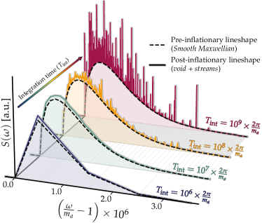
Figure 2: An illustration of how minicluster streams would manifest in the axion lineshape—the spectral energy distribution of the axion field in terms of its oscillation frequency $\omega$. The form of this lineshape is approximately Maxwellian, and the frequency resolution is inversely proportional to the duration of the observation, $T_{\rm int}$, from which the spectrum is obtained via a discrete Fourier transform. If $T_{\rm int}$ is short, as it would be for a resonant haloscope operating in discovery mode while scanning over a wide range of masses, then the minicluster streams are not picked up, and the signal is indistinguishable from a smooth halo. However, the longer these samples become, the finer the spectral resolution, thereby resolving the streams.

Impact on signals in axion haloscopes.—We now know how many streams we expect to have around us at any one time, and so we can draw a sample of this size and predict how this would look in a haloscope experiment. First, we must build the velocity distribution of axions. In the voids, we can safely assume the halo is described by the smooth, fully virialised distribution function of the SHM Evans:2018bqy modelled as an isotropic Gaussian. An experiment observes this after a Galilean boost into our frame of reference, moving at a velocity $\mathbf{v}_{\rm lab}(t)$ with respect to the Galactic centre. The expression is,

$$f_{\mathrm{void}}(\mathbf{v})=\frac{1}{\left(2\pi\sigma_{\mathrm{void}}^{2}\right)^{3/2}}\exp\left(-\frac{\left(\mathbf{v}+\mathbf{v}_{\rm lab}\right)^{2}}{2\sigma_{\mathrm{void}}^{2}}\right)$$ (7)

where $\sigma_{\rm void}=v_{\rm circ}/\sqrt{2}\approx 165$ km/s is the velocity dispersion of the SHM. We take $\mathbf{v}_{\rm lab}=(11.1,235.2,7.3)\,{\rm km/s}+\mathbf{v}_{\oplus}(t)$ Evans:2018bqy in the same Galactocentric cartesian coordinate system as Fig. 1, where $\mathbf{v}_{\oplus}(t)$ is the Earth’s velocity, see e.g. McCabe:2013kea ; Mayet:2016zxu .

Following past literature Freese:2003tt ; OHare:2014nxd ; Foster:2017hbq ; OHare:2018trr ; OHare:2019qxc ; Ko:2023gem , we take the stream velocity distribution to have the same Gaussian form. We make the replacement $\mathbf{v}_{\rm lab}\to\mathbf{v}_{\rm lab}-\mathbf{v}_{\rm str}$ to account for the fact that the stream is streaming with its own velocity, and $\sigma_{\rm void}\to\sigma_{\rm str}\gtrsim\sigma_{\rm mc}$. Because the values of $\sigma_{\rm str}$ are very small (even accounting for additional heating during the energy injection and tidal elongation Schneider:2010jr ), the signal they would leave in haloscopes is extremely narrow in frequency, so our results are not influenced by this ad hoc choice of velocity distribution.

We now relate this velocity distribution to the signal measured by a typical axion haloscope known as the axion lineshape. The axion field’s oscillations are highly coherent, in keeping with its description as cold DM. Within a “coherence time”, the axion field will appear to oscillate at a single frequency $\omega\approx m_{a}(1+v^{2}/2)$ where $v\sim 10^{-3}c$ is some speed drawn from the velocity distribution. This frequency is then the frequency at which some induced signal will usually be driven, e.g. the electromagnetic field inside a resonant cavity, or the oscillating pseudo-magnetic field experienced by a sample of nuclear spins Gramolin:2021mqv . The axion’s velocity distribution causes this frequency to evolve on timescales longer than coherence time, related to the spread in velocities: $\tau_{\rm coh}\sim 1/m_{a}\sigma^{2}_{\rm void}\sim 10^{6}m^{-1}_{a}\sim{\rm 0.01ms}(100\mu{\rm eV}/m_{a})$. When these oscillations are measured over timescales much longer than this, then the discrete Fourier transform of that measurement will have a spectral density related to the distribution of component frequencies. For a measurement time, $T_{\rm int}$, the power spectrum $S(\omega)$, is resolved in frequency to the level $\Delta\omega=2\pi/T_{\rm int}$. Therefore, if $T_{\rm int}>10^{6}\times 2\pi/m_{a}$ (i.e. longer than a million oscillation periods) then we expect the axion’s lineshape to be resolved Turner:1990qx ; Derevianko:2016vpm ; Foster:2017hbq ; OHare:2017yze .

To illustrate this, and show the impact of the streams on the lineshape, let us define a simplified version of a signal power spectrum by discretising the distribution of component frequencies into bins of width $\Delta\omega$,

$$S(\omega_{i})=\int_{\omega_{i}-\frac{1}{2}\Delta\omega}^{\omega_{i}+\frac{1}{2}\Delta\omega}\big{(}\rho_{\rm str}f_{\rm str}(\omega)+\rho_{\rm void}f_{\rm void}(\omega)\big{)}\textrm{d}\omega$$ (8)

where $f(\omega)$ is the same as the velocity distributions written above but with velocity transformed to frequency. Note that there will also be a fundamental stochasticity to the amplitudes in each bin due to the incoherent sums of axion waves with unrelated phases going into each frequency bin Derevianko:2016vpm ; Foster:2017hbq . Figure 2 compares the smooth Maxwellian case (as in, for example, the pre-inflationary cosmology) against the case when we have streams in the signal. The two will become strikingly different once the signal is measured for timescales longer than around a thousand coherence times (or equivalently, a million oscillation periods), though a precise statement about detectability depends upon the type of experiment and its signal-to-noise—see e.g. Foster:2017hbq ; OHare:2017yze ; Knirck:2018knd for studies that address this idea.

As well as showing up as sharp features in short-duration measurements, the lineshape will also evolve in amplitude over human timescales as we traverse the streams. Sampling over all of our streams and randomising our trajectory through them, we find that they would typically persist for around $\Delta t=30^{+23}_{-11}\,{\rm years}$ (median and 68% containment). However, since we expect several hundred to a thousand of them present in the lineshape at one time, the timescale over which the signal is therefore expected to vary is much shorter, on the order of tens of days. Time-varying and/or ultra-narrowband signals like these are already being searched for by existing haloscope collaborations in high-resolution variants of their standard analyses, e.g. Duffy:2005ab ; ADMX:2006kgb ; ADMX:2023ctd , so in light of our results, we advocate that these efforts continue.

Conclusions.—In this letter we have evaluated the extent to which axion haloscopes are doomed under the post-inflationary scenario when axions find themselves bound up inside of small substructures. We have modelled miniclusters encountering stars as they orbit the MW and have found that, as a result of tidal disruption, the density of DM around us in the solar neighbourhood is refilled to around 80% of the 100-pc-scale average DM density $\rho_{\rm DM}\approx 0.4$ GeV cm^-3 which is usually adopted in experimental analyses. Combined with an estimate of the density of DM that never ended up bound inside of miniclusters Eggemeier:2022hqa , this boosts the signal up to around 90% of the commonly assumed value, or in other words: axion haloscopes may not be doomed. The streams also give rise to a multitude of sharp peaks in the axion lineshape which could be resolved when the axion is discovered—a smoking gun for the post-inflationary scenario.

Acknowledgements.— We thank Benedikt Eggemeier, David Marsh and Yvonne Wong for helpful discussions. CAJO is funded via the Australian Research Council, grant number DE220100225. The work of J.R. is supported by Grants PGC2022-126078NB-C21 funded by MCIN/AEI/ 10.13039/501100011033 and “ERDF A way of making Europe” and Grant DGA-FSE grant 2020-E21-17R Aragon Government and the European Union - NextGenerationEU Recovery and Resilience Program on ‘Astrofísica y Física de Altas Energías’ CEFCA-CAPA-ITAINNOVA. This article is based upon work from COST Action COSMIC WISPers CA21106, supported by COST (European Cooperation in Science and Technology). Most of this work first appeared in G.P.’s PhD thesis submitted in September 2023.

I Minicluster properties from early-Universe simulations

In this section, we give further details on the simulations that inspire our initial population of miniclusters and detail the structural parameters that are necessary to model their subsequent disruption. As described in Refs. Eggemeier:2022hqa ; Pierobon:2023ozb we evolve a realistic configurations of the axion DM field within the redshifts $10^{16}\lesssim z\lesssim 10^{2}$.

The distribution of miniclusters can either be predicted using the spectrum of density fluctuations $\Delta^{2}$ left behind following the collapse of the axion string-wall network, or they can obtained directly by performing an N-body simulation. Recently, Ref. Pierobon:2023ozb demonstrated how both the mass distribution and internal structures of miniclusters vary when adopting different treatments of the early Universe dynamics—in particular the modelling of axion strings. Due to these outstanding uncertainties, current simulations Eggemeier:2019jsu ; Xiao:2021nkb ; Pierobon:2023ozb are unfortunately unable to conclusively identify a universal density profile for all forming miniclusters. For this study we have chosen to adopt the early Universe modelling of direct simulations at large string tension (dubbed high-$\kappa$) from Ref. Pierobon:2023ozb , which best describes the string-wall network with respect to previous works.

Uncertainties aside, in more general terms however, recent N-body simulations are able to show that the NFW profile fits well the high-mass end of the miniclusters mass function corresponding to hierarchical mergers of smaller miniclusters. Whereas on the low-mass end, consisting of miniclusters that remain isolated after their initial collapse, power-law profiles fit much better. These two types of minicluster can be seen in Fig. S1 where we display the halo mass function at a redshift of 499, taken from the N-body simulations presented in Ref. Pierobon:2023ozb . The non-linear regime refers to those miniclusters that promptly collapse and then do not undergo significant mergers, whereas the high mass tail which grows out of the hierarchical merger of many initially isolated miniclusters has a spectrum well-described by Gaussian white noise, hence why it is referred to the white-noise regime. We describe how we model each of these now in turn.

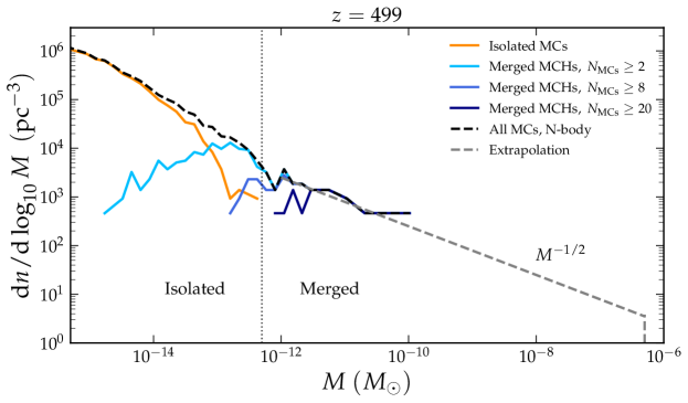
Figure S1: Halo mass function at a redshift of 499, resulting from an N-body simulation that used initial conditions calculated by a high-string-tension lattice simulation (high-$\kappa$, as in Ref. Pierobon:2023ozb ). The total mass function for all miniclusters and minicluster halos (MCHs) is shown as a dashed line, while the coloured lines show the individual mass functions for minicluster halos comprised of different numbers of individual miniclusters. Our final results are heavily dominated by the upper end of this mass function comprised of the mergers of many miniclusters. This regime, described well by Gaussian white-noise consists entirely of merged NFW halos of masses that should extend up to $\sim 5\times 10^{7}~{}M_{\odot}$.

I.1 Isolated miniclusters

Isolated miniclusters are defined to be the early-forming ($z\gtrsim z_{\rm eq}$) bound objects associated with the large nonlinear overdensities left by inhomogeneities in the axion field, which in turn result directly from the collapse of the string-wall network. We find that isolated miniclusters occupy the mass distribution for masses $M\lesssim 10^{-12}~{}M_{\odot}$ and have radii $R\lesssim 10^{-6}$ pc.

Isolated miniclusters can be fit well using a power-law profile in terms of an index $\tilde{\alpha}$,

$$\rho_{\rm PL}(r)=Cr^{-\tilde{\alpha}},\quad\quad C=\frac{3\langle\rho\rangle}{3-\tilde{\alpha}},$$ (S1)

where $\langle\rho\rangle$ is the average energy density of the minicluster. In our simulations, they typically exhibit power-law profiles with index $\tilde{\alpha}=9/4$ at $z\sim z_{\rm eq}$. However at $z\sim 500$ the value shifts to an average $\langle\tilde{\alpha}\rangle=2.71$. Densities are sampled from a Gaussian distribution built using mean and standard deviation of simulation data of small-mass miniclusters. We assume the isolated miniclusters occupy the range $M\in[10^{-16},10^{-12}]~{}M_{\odot}$, and have a mass function (number density of miniclusters versus mass) given by $\textrm{d}n/\textrm{d}\log M\propto M^{\gamma}$, with $\gamma=-0.8$.

Isolated miniclusters represent about 70% of the total by number—resulting as a consequence of the mass cutoff that divides what constitutes an isolated versus a merged minicluster. This is the seen in high-$\kappa$ N-body simulations, first described in Ref. Pierobon:2023ozb . We mention these details for clarity, but as discussed in the main text, and above, we ultimately find that our key result is not impacted by our modelling of the isolated miniclusters, and our results are unchanged even if we make extreme departures from any of the assumptions we have made about them.

I.2 Merged miniclusters

Much more important are the merged minicluster halos form in the white-noise regime, namely fluctuations on scales $k\ll L_{1}^{-1}$. Defining $M_{1}$ as the characteristic mass defined as

$$M_{1} =\frac{4\pi}{3}(\pi L_{1})^{3}$$ (S2)

$$\simeq 1.76\times 10^{-10}\,M_{\odot}~{}\left(\frac{100~{}\mu{\rm eV}}{m_{a}}\right)^{0.51}.$$ (S3)

where $m_{a}$ is the axion mass, merged miniclusters will have masses $M\gtrsim M_{1}$, for which the spectrum is well-described by Gaussian white-noise Enander:2017ogx .

Merged minicluster halos around and above the characteristic mass evolve towards a Navarro-Frank-White (NFW) Navarro:1995iw profile, which is given by the following expression,

$$\rho_{\rm NFW}(r)=\frac{\rho_{s}}{(r/r_{s})(1+r/r_{s})^{2}},$$ (S4)

with $r_{s},\rho_{s}$ scale radius and scale density, respectively. To model our miniclusters, we use numerical results of the white-noise N-body simulations from Ref. Xiao:2021nkb , which found a scale radius and concentration as a function of the minicluster mass and redshift, $z$.

$$r_{s}(M)=2.6~{}{\rm pc}\left(\frac{A_{\Delta^{2}}M_{1}}{10^{-11}~{}M_{\odot}h^{-1}}\right)^{-1/2}\left(\frac{M}{10^{-6}~{}M_{\odot}h^{-1}}\right)^{5/6},$$ (S5)

$$c(z)=\frac{r_{s}}{R}=\frac{1.4\times 10^{4}}{(1+z)}\left(\frac{M}{A_{\Delta^{2}}M_{1}}\right)^{-1/2}.$$ (S6)

From this, the radius at which the profile is truncated so that it contains can be parameterised as Xiao:2021nkb

$$R(M)\equiv R_{\rm 10}\left(\frac{M}{10^{-10}~{}M_{\odot}}\right)^{1/3}\simeq 0.55\,{\rm mpc}~{}\left(\frac{M}{10^{-10}~{}M_{\odot}}\right)^{1/3}.$$ (S7)

which we adopt to model our minicluster, taking $z=19$. Note that the overall scale for this radius is almost a factor of three larger than that assumed by Kavanagh et al. Kavanagh:2020gcy in their minicluster disruption study. Their value is equivalent to a concentration parameter of only $c=100$, which they argue would be a result of rapid initial truncation by tidal stripping as the miniclusters originally fell into the MW halo. Instead, we implement this continual tidal stripping by the MW halo inside of our perturbation loop, following the formulae in Appendix A of Ref. Kavanagh:2020gcy . Nonetheless, this overall truncation scale of the profile ends up impacting some of our results. Instead of parameterising this uncertainty in terms of $c$, which does not directly enter our results, we instead parameterise the truncation radius using the prefactor in the expression above. We define this to be $R_{10}$ and will show results as a function of this quantity in Sec. IV.

For our NFW halos, the individual mean densities are sampled from a normal distribution with mean and variance according to the N-body data Pierobon:2023ozb . We sample masses in the range $M\in[10^{-12},5\times 10^{-7}]~{}M_{\odot}$ according to halo-mass function ${\rm d}n/{\rm d}\log M\propto M^{\gamma}$ with $\gamma=-0.5$. The upper mass cut-off has been estimated as $\sim 0.03\langle\rho\rangle L_{1}^{3}z_{\rm eq}^{2}$ from the Press-Schechter estimate of the variance obtained from numerical simulations in Pierobon:2023ozb .

Before moving on, it is worth remarking here briefly that our results are largely insensitive to the question of whether or not miniclusters host small solitonic cores called axion stars Visinelli:2017ooc . Numerous recent studies have suggested that all gravitationally bound structures of a bosonic field ought to develop these cores Levkov2018 ; Eggemeier:2019jsu ; Chen:2020cef , which may survive and even grow during mergers Du:2023jxh . Assuming the core-halo mass relation seen in simulations of the Schrodinger-Poisson system Schive2014_PRL is universal (i.e. down to minicluster masses Eggemeier:2019jsu ), we can evaluate it at the present day to yield the following relationship with the minicluster mass,

$$M_{\rm star}=5.58\times 10^{-17}\,M_{\odot}\left(\frac{100\,\mu{\rm eV}}{m_{a}}\right)\left(\frac{M}{10^{-10}\,M_{\odot}}\right)^{1/3}$$ (S8)

Some intrinsic diversity away from this relation has been seen in some simulations, but we are primarily interested in the ratio between the core and halo mass at an order-of-magnitude level Nori:2020jzx ; Chan:2021bja ; Zagorac:2022xic .

Axion stars have presented a potentially problematic theoretical uncertainty in previous studies that focused on the survival of miniclusters. Since the axion star could potentially prevent miniclusters from being totally stripped. However, we notice here that the total mass contained in the axion star is vastly subdominant, and all of our results depend dominantly on the loosely bound outer layers of the high-mass merged miniclusters which are stripped early on in the evolution. Hence we do not need to worry about whether or not miniclusters host axion stars, and accounting for presence in the cores of our miniclusters, or implementing cuts on stripped miniclusters which would host unphysically large axion stars (as in Ref. Kavanagh:2020gcy ), would not change any of our results.

II Galactic stellar density model

The number of stars encountered within an impact parameter of $b_{\rm max}$ is given by the integral along the minicluster trajectory:

$$N_{\rm enc}=\int_{0}^{t_{\rm MW}}{\rm d}t~{}n_{\star}(t)v(t)\pi b^{2}_{\rm max}\,.$$ (S9)

To get the stellar number density, $n_{\star}(t)$ we write down a model for the galactic stellar mass density and choose a characteristic star mass $M_{\star}=1~{}M_{\odot}$. Because the disruption probability is proportional to the number density of stars times their mass, including a detailed stellar mass function is not expected to change our conclusions if we keep the volume and total mass fixed Dokuchaev –and in any case, $1~{}M_{\odot}$ is a very typical star mass for standard stellar initial mass functions.

Our stellar density model, as in Refs. Kavanagh:2020gcy ; Dokuchaev , consists of a bulge and disk, of which the latter has two components, labelled as thick and thin:

$$\rho_{\star}=\rho_{\rm bulge}+\rho^{(t)}_{\rm disk}+\rho^{(T)}_{\rm disk}\,.$$ (S10)

The bulge density profile is modelled as a truncated power-law Binney:1996sv ; Bissantz:2001wx ; Kavanagh:2020gcy

$$\rho_{\rm bulge}(r,z)=\rho_{{\rm bulge},0}\frac{\exp(-r^{\prime}/r_{\rm cut})^{2}}{1+(r^{\prime}/r_{0})^{1.8}},\quad r^{\prime}=\sqrt{(r^{2}+4z^{2})}$$ (S11)

where $r=\sqrt{x^{2}+y^{2}}$ is the cylindrical radius in the disk-plane, and $z$ the height above the disk plane. The central density is $\rho_{{\rm bulge},0}\simeq 99.5~{}M_{\odot}/{\rm pc}^{3}$, and the radial scales are $r_{0}=0.075$ kpc and $r_{\rm cut}=2.1$ kpc.

Both the thick and the thin stellar disk profiles are modelled by a double exponential Dehnen:1996fa

$$\rho_{\rm disk}^{t,T}(r,z)=\frac{\Sigma^{t,T}_{\star}}{z^{t,T}}\exp\left(-\frac{r}{r^{t,T}}-\frac{Z}{z^{t,T}}\right),$$ (S12)

where $r^{t,T},z^{t,T}$ are the scale radius and height, and $\Sigma^{t,T}_{\star}$ are the stellar surface densities:

$$z^{t} =0.3~{}{\rm kpc},\quad r^{t}=2.90~{}{\rm kpc}\quad\Sigma^{t}_{\star}=816.6~{}M_{\odot}~{}{\rm pc}^{-2},$$ (S13)

$$z^{T} =0.9~{}{\rm kpc},\quad r^{T}=3.31~{}{\rm kpc}\quad\Sigma^{T}_{\star}=209.5~{}M_{\odot}~{}{\rm pc}^{-2}.$$ (S14)

Our results are not sensitive to the detailed parameterisation of the stellar density, and varying any of these numbers within up to a few tens of percent leaves our results generally unaffected.

III Minicluster disruption computation

Here we provide a brief account of the disruption computation, though for further discussion of the motivation and justification behind this treatment, we refer to Ref. Kavanagh:2020gcy .

Once an encounter time ($t_{\rm enc}$), star mass ($M_{\star}$), and impact parameter ($b$) have been chosen, the first step is to compute the energy injected into the minicluster by that encounter. Under the distant tide and the impulse approximations assumptions, the energy injection can be written as 1958ApJ…127…17S :

$$\Delta E\simeq\left(\frac{2GM_{*}}{b^{2}v_{\rm rel}}\right)^{2}\frac{M\langle R^{2}\rangle}{3},$$ (S15)

where $\langle R^{2}\rangle$ is the minicluster mean-squared radius. This can be expressed in terms of a structural parameter, $\alpha$,

$$\alpha^{2}=\frac{\langle R^{2}\rangle}{R^{2}}=\frac{4\pi}{MR^{2}}\int_{0}^{R}{\rm d}rr^{4}\rho(r)\,.$$ (S16)

For an NFW minicluster with concentration $c=100$, Refs. Kavanagh:2020gcy ; Shen:2022ltx find $\alpha^{2}=0.13$. For the power-law profile, we use $\alpha^{2}=0.27$ Kavanagh:2020gcy .

Equation (2) must then be compared to the binding energy of the minicluster, $E_{b}$, which is given by the familiar $\sim GM/R^{2}$ up to some factor $\beta$, that encodes details of the internal structure. We define it via,

$$E_{b}\simeq\beta\frac{GM^{2}}{2R},$$ (S17)

where the structural parameter is

$$\beta^{2}=\frac{4\pi R^{2}}{M}\int_{R_{\rm min}}^{R}{\rm d}r\rho(r)\,.$$ (S18)

If the energy injected into the minicluster by the star’s tidal field exceeds the binding energy, we expect the minicluster to be disrupted. However, since most encounters inject $\Delta E\ll E_{b}$, we deal with perturbations giving rise to small mass losses $\Delta M$.

In the distant tide approximation, the normalised injected energy increases proportionally to $R^{2}$:

$$\Delta\mathcal{E}(R)=-\frac{\Delta E}{M}\frac{R^{2}}{\langle R^{2}\rangle},$$ (S19)

where $\mathcal{E}=-E/m_{a}$ is the energy per unit mass. The mass that is then left unbound to the cluster following this injection is then given by the total mass in axions with energies smaller than $\Delta\mathcal{E}$ Kavanagh:2020gcy

$$\Delta M(\Delta E)\equiv M(<\Delta\mathcal{E})=\int_{\mathcal{E}<\Delta\mathcal{E}(R)}\mathrm{d}^{3}\mathbf{x}\,\mathrm{d}^{3}\mathbf{v}f(\mathcal{E})$$ (S20)

In our computation, we use a numerical interpolation of this mass loss function, $\Delta M(\Delta E)$, given in Ref. Kavanagh:2020gcy . The functional dependence of the mass loss is in rough agreement with Ref. Shen:2022ltx , who instead performed idealised N-body simulations of an NFW halo interacting with a $1~{}M_{\odot}$ star. We notice mild disagreement only for $\Delta E/E_{b}\lesssim 10^{-2}$ and both models approach $\Delta M/M\sim 1$ as expected for very large energy injections $\Delta E/E_{b}\gg 1$ which can totally disrupt the minicluster, though these occur rarely. Reference Shen:2022ltx limits the treatment to NFW initial profiles only, while the modelling of Ref. Kavanagh:2020gcy can be extended to different profiles.

The initial energy of the minicluster before the energy injection is given by the sum of the kinetic energy ($1/2M\sigma_{\rm mc}^{2}$) and binding energy ($E_{b}$):

$$E_{i}=\left(\frac{\kappa}{2}-\beta\right)\frac{GM^{2}}{R}$$ (S21)

where $\kappa=1.73,\,3.54$—for isolated and merged miniclusters respectively—parameterises the velocity dispersion as follows,

$$\sigma_{\rm mc}^{2}=\kappa\frac{GM}{R}\,.$$ (S22)

Following energy conservation, the final minicluster energy after $\Delta E$ has been injected can be written as,

$$E_{f}=E_{i}+(1-f_{\rm ej})\Delta E-E^{\rm unb}_{i}\,,$$ (S23)

$f_{\rm ej}(\Delta E)$ is the fraction of the imparted energy that becomes unbound and $E^{\rm unb}_{i}(\Delta E)$ the energy originally possessed by those axions that became unbound. Bound axions are those satisfying the integral cutoff in Eq.(S20), and unbound axions the reverse. Like with the function $\Delta M(\Delta E)$ we adopt interpolations of $f_{\rm ej}(\Delta E)$ and $E^{\rm unb}_{i}(\Delta E)$ provided by Ref. Kavanagh:2020gcy .

After each encounter, and before moving to the next one, the minicluster mass and radius are updated to,

$$M\rightarrow M-\Delta M,\quad\quad R\rightarrow\left(\frac{\kappa}{2}-\beta\right)\frac{G(M-\Delta M)^{2}}{E_{f}}\,.$$ (S24)

We continue to perturb each minicluster through its $N_{\rm enc}$ encounters until either it is fully unbound ($E_{f}>0$) or we have reached the end of the orbit.

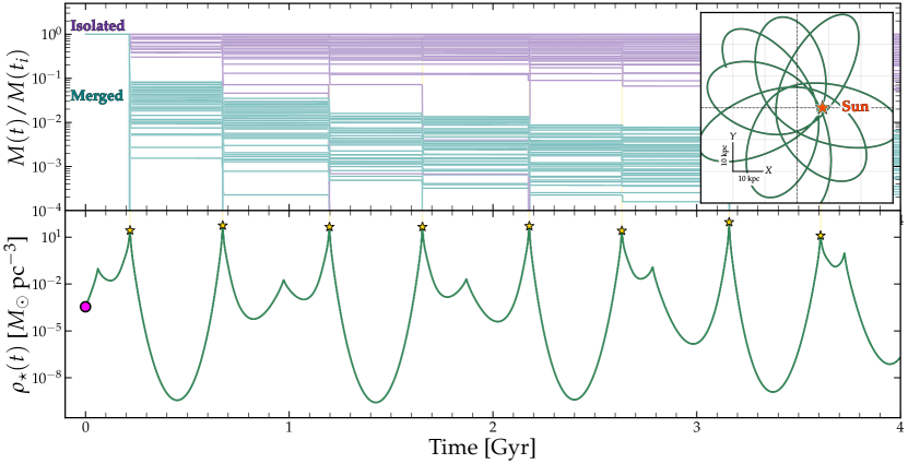
Figure S2: Upper panel: the remaining masses of miniclusters for the first 4 Gyr of their evolution as they orbit the Milky Way, relative to their initial mass $M(t_{i})$. The teal lines show 100 randomly sampled merged miniclusters (high-mass, NFW profiles), whereas purple is used for isolated miniclusters (low-mass, power-law profiles). All miniclusters are evolved along the same orbit. Lower panel: The stellar density for the chosen orbit. The disk-crossing times are marked with yellow stars, which coincide with the events of major mass loss for both types of minicluster. Inset: a projection of the trajectory of this chosen orbit in galactocentric $(X,Y)$ coordinates, where the Sun is located at (8,0) kpc.

In Fig. S2 we show the stellar density as a function of time, $\rho_{\star}(t)$ for a random orbit ending at the Solar position today $t=t_{\rm MW}$ (we zoom in on the initial 5 Gyr for visual clarity, although in our calculation we evolve each minicluster until today). The orbit has a mean galactocentric radius of $\sqrt{X^{2}+Y^{2}}=22$ kpc and a mean inclination of $\sin^{-1}(Z/\sqrt{X^{2}+Y^{2}})=21^{\circ}$. In the upper panel, we show the gradual loss in mass as a function of time normalised to the minicluster’s initial mass. The miniclusters are randomly sampled in mass from their mass function (see S.M. I), but all follow the same orbit, an $X$-$Y$ projection of which is shown in the inset panel to the right. The mass loss exhibits a step-like behaviour for this orbit due to the exponential enhancement in the stellar density whenever the orbit crosses the disk plane $Z=0$. We see here clearly that the merged NFW-profile miniclusters lose a much larger fraction of their mass and over a much shorter timescale—particularly in the first disk-crossing. In contrast, many isolated power-law miniclusters survive with an $\mathcal{O}(1)$ fraction of their mass today.

IV Impact of modelling uncertainties

To provide further intuition behind the results presented in the main text, in this section, we make some back-of-the-envelope estimates that explain why we should expect the DM density to be mostly replenished by the disruption of the most massive miniclusters. Doing this will also allow us to evaluate the possible effects (if any) that changing our modelling assumptions might have on our main result.

Let us start with a simplified description of the situation wherein the DM is composed entirely of merged miniclusters, which we assume are all disrupted in their entirety. This is already very close to our fiducial analysis since most of the mass is in the high-mass merged miniclusters anyway and, as we have seen (e.g. in Fig. S2), the stellar disruption process causes them to lose the majority of their mass quite quickly. If we now further simplify the situation and assume all the resulting streams have the same volume $V_{\rm str}$ and the same mass $M$ then the expected number of streams overlapping at a single point is,

$$\langle N_{\rm str}\rangle\approx N_{\rm mc}\frac{V_{\rm str}}{V}=\frac{\rho_{\rm DM}V_{\rm str}}{M}\,,$$ (S25)

where in the second step we have rewritten the local galactic DM density we are required to saturate as $\rho_{\rm DM}=N_{\rm mc}M/V$. The expectation value for the density that we measure on Earth is then just the sum of all of the individual stream densities: $\langle\rho_{\rm obs}\rangle=\langle N_{\rm str}\rangle\rho_{\rm str}=N_{\rm str}M/V_{\rm str}$. Notice that if we substitute in $\langle N_{\rm str}\rangle$ from above we get back $\langle\rho_{\rm obs}\rangle=\rho_{\rm DM}$. We enforce this because when averaging the DM densities observed at many different points in a volume $V\gg V_{\rm str}$ should give us back DM density defined on that scale.

So the possible values of $\rho_{\rm obs}$ follow a binomial distribution with a mean of $\rho_{\rm DM}$. When $\langle N_{\rm str}\rangle$ is large, the central limit theorem dictates that the distribution of $\rho_{\rm obs}$ is a Gaussian centred on $\rho_{\rm DM}$. However in the opposite extreme, when $\langle N_{\rm str}\rangle\lesssim 1$ (for example if the miniclusters were not disrupted for whatever reason) the mean is still $\rho_{\rm DM}$, but only because the high probability to observe $\rho_{\rm obs}=0$ is balanced against the very rare probability to observe a hugely enhanced density $\rho_{\rm obs}=\rho_{\rm str}\gg\rho_{\rm DM}$ because the stream volumes would have to be very small to cause $N_{\rm str}\lesssim 1$.

So for this reason, the pertinent result is not the expectation value of the density, because as a result of conserving the total mass of DM on large scales this is always $\rho_{\rm DM}$ by construction. Instead, we must consider the distribution of $\rho_{\rm obs}$, which is dictated by $N_{\rm str}$.

So to see which regime we are in, whilst also evaluating the effects of changing some of our assumed input parameters, let us develop a simple analytic estimate for the expected number of observed streams. Starting with the formula for the stream volume, parametrically this can be modelled as,

$$V_{\rm str}\gtrsim\pi R^{2}\sigma_{\rm mc}(t_{\rm MW}-t_{\rm enc})\,,$$ (S26)

where $4\sigma_{\rm mc}(t_{\rm MW}-t_{\rm enc})$ is roughly the stream length assuming a disruption happens (as we observe here) very quickly, i.e. after only a few disk crossings. We use a $\gtrsim$ sign because the minicluster velocity dispersion gives us a lower limit on the stream’s velocity dispersion. The latter is expressed as $\sigma_{\rm mc}^{2}=\kappa GM/R$, as in Eq.(S22) above.

If we now plug in our formula for the radii of merged miniclusters $R(M)=R_{10}(M/10^{-10}\,M_{\odot})^{1/3}$ (as in Eq.(S7)), we see that the dependence on $M$ in the stream number $N_{\rm str}=\rho_{\rm DM}V_{\rm str}/M$ drops out entirely, giving us,

$$N_{\rm str}=\frac{R_{10}^{3/2}}{(10^{-10}\,M_{\odot})^{1/2}}4\pi\sqrt{G\kappa}\rho_{\rm mc}(t_{\rm MW}-t_{\rm enc})\gtrsim 200\,,$$ (S27)

where we assign $\rho_{\rm mc}=\rho_{\rm DM}(1-f_{\rm void})\approx 0.01~{}M_{\odot}\,{\rm pc}^{-3}$ as the portion of the DM density that was originally bound inside miniclusters (i.e. not in the minivoids). To evaluate this expression, we have taken the average mass-loss-weighted encounter time from our simulations of $t_{\rm enc}\sim 3$ Gyr, which gives us a number strikingly close to our fiducial numerical result.

So referring back to our statements above about the distribution of $\rho_{\rm obs}$, the key point to highlight is that we are quite firmly in the regime $N_{\rm str}\gg 1$, especially because we have fixed the stream length $\sigma_{\rm mc}(t_{\rm MW}-t_{\rm enc})$ to be the smallest that we expect it to grow to. We may account for additional heating of the axions to dispersions larger than $\sigma_{\rm mc}$, but will only act to increase this number, further reinforcing the fact that we expect there to be a large number of streams overlapping at our position.

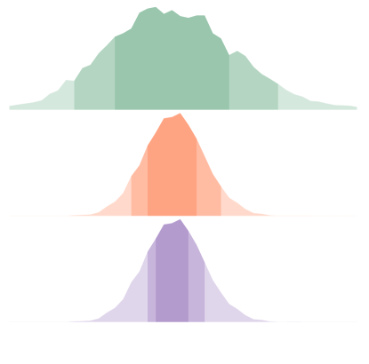
Figure S3: Independence of our final result on the minicluster mass-radius relation, parameterised by the radius scale $R_{10}$, and how much the stream’s velocity dispersion is additionally heated from its initial value given by the minicluster’s velocity dispersion. In all cases we see that the median value of observed density is roughly the same, with the primary role of these parameters being to change the expected number of overlapping streams, and hence the variance in the density, as opposed to its expectation value. The number of streams observed in the three examples ranges from $N_{\rm str}=63,\,246,\,$ and $547$, from the top to bottom, and a factor of 10 larger for the $\sigma_{\rm str}=10\sigma_{\rm mc}$ case.

This estimate also reveals a general insensitivity of the stream number to many model parameters. So we expect $N_{\rm str}\gg 1$ to remain the case if we allow the mass function, density profiles, mass-radius relation, and abundance of merged miniclusters to vary over any reasonable range. We can see this from our simple analytic estimate, but have confirmed this remains the case in our full simulation as well which accounts for variable disruption probabilities as a function of $M$, varying disruption times as a function of the minicluster orbit, as well as the varying densities along the stream. In fact, the reason our numerical analysis leads to a median $\rho_{\rm obs}$ slightly smaller than $\rho_{\rm DM}$ is because of these additional details.

Nevertheless, our full numerical results are also generally insensitive to most of our more crude assumptions. To show a few explicit examples of factors that cause the result to change the most, Fig. S3 shows multiple versions of our final result—the distribution in the sum of the stream densities, $\Sigma\rho_{\rm str}$—for multiple different choices for the initial sizes of the miniclusters $R_{10}$ (or equivalently, their concentration parameters, $c$), as well as for different stream heating factors beyond the most conservative case where $\sigma_{\rm str}=\sigma_{\rm mc}$. We see that even with these alternative choices, the median value of the density is mostly unchanged, and these quantities instead only affect the variance in the distribution (as expected because these quantities affect $\langle N_{\rm str}\rangle$).

V Impact of minicluster halo substructure

As argued in the previous section, the conclusion that we expect the local DM density to be almost saturated after minicluster disruption can be considered reasonably robust, assuming our result that the merged miniclusters lose the majority of their mass holds up. However, it is this final issue that is really the only factor that could change our result in any substantial way. If the merged miniclusters are in fact more stable than the NFW halos that we have modelled them as, then it is possible they hold on to more of their mass and not spread it over such large volumes. One way in which this might not be captured in our treatment is if the merged miniclusters are not smooth NFW profiles but rather retain a degree of substructure from the isolated miniclusters that created them. We identify this as the primary remaining theoretical uncertainty that should be resolved with high-resolution (i.e. longer timescale) simulations that can evolve the minicluster halos to lower redshifts.

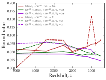
Figure S4: Bound fraction of axions within each minicluster halo (host), excluding the main virialised part, and as a function of the host mass.

So are our simulated minicluster halos actually just clusters of compact miniclusters? Minicluster halos are partially made by merging and accretion of isolated MCs. It is crucial for what follows to know the fraction of the mass of the MCH that is smoothly distributed and the fraction that it is still retained in compact MCs. This can be extracted from the numerical simulations to some extent using the subfind algorithm implemented in the gadget-4 Springel:2020plp code. From our recent N-body simulations (see Sec. I) we calculate the fraction of axions contained in subhalos for each host (i.e., minicluster halo) identified by the friend-of-friends (FOF) algorithm. In this calculation we however do not consider the main virialised halo (the first subhalo within the FOF group), since the latter will not contain itself additional substructure. As seen in Fig. S4, we find that only $\sim 10\%$ of the MCHs are composed of smaller virialised orbiting miniclusters. As expected, we confirm that high-mass MCHs have comparatively more substructure than low-mass MCHs. This lends further confidence that our modelling of these larger miniclusters as smooth NFW profiles can be considered reasonably accurate.

References

- (1) L. Di Luzio, M. Giannotti, E. Nardi and L. Visinelli, The landscape of QCD axion models, Phys. Rept. 870 (2020) 1 [2003.01100].
- (2) F. Chadha-Day, J. Ellis and D. J. E. Marsh, Axion dark matter: What is it and why now?, Sci. Adv. 8 (2022) abj3618 [2105.01406].
- (3) I. G. Irastorza and J. Redondo, New experimental approaches in the search for axion-like particles, Prog. Part. Nucl. Phys. 102 (2018) 89 [1801.08127].
- (4) Y. K. Semertzidis and S. Youn, Axion dark matter: How to see it?, Sci. Adv. 8 (2022) abm9928 [2104.14831].
- (5) C. B. Adams et al., Axion Dark Matter, in 2022 Snowmass Summer Study, 3, 2022, 2203.14923.
- (6) R. D. Peccei and H. R. Quinn, CP conservation in the presence of instantons, Phys. Rev. Lett. 38 (1977) 1440. [,328(1977)].
- (7) R. D. Peccei and H. R. Quinn, Constraints Imposed by CP Conservation in the Presence of Instantons, Phys. Rev. D 16 (1977) 1791.
- (8) S. Weinberg, A New Light Boson?, Phys. Rev. Lett. 40 (1978) 223.
- (9) F. Wilczek, Problem of Strong p and t Invariance in the Presence of Instantons, Phys. Rev. Lett. 40 (1978) 279.
- (10) J. E. Kim and G. Carosi, Axions and the Strong CP Problem, Rev. Mod. Phys. 82 (2010) 557 [0807.3125]. [Erratum: Rev. Mod. Phys.91,no.4,049902(2019)].
- (11) J. E. Kim, Weak interaction singlet and Strong CP invariance, Phys. Rev. Lett. 43 (1979) 103.
- (12) M. A. Shifman, A. I. Vainshtein and V. I. Zakharov, Can Confinement Ensure Natural CP Invariance of Strong Interactions?, Nucl. Phys. B 166 (1980) 493.
- (13) M. Dine, W. Fischler and M. Srednicki, A simple solution to the Strong CP Problem with a harmless axion, Phys. Lett. B 104 (1981) 199.
- (14) A. R. Zhitnitsky, On Possible Suppression of the Axion Hadron Interactions. (In Russian), Sov. J. Nucl. Phys. 31 (1980) 260. [Yad. Fiz.31,497(1980)].
- (15) L. Fleury and G. D. Moore, Axion dark matter: strings and their cores, JCAP 01 (2016) 004 [1509.00026].
- (16) V. B. . Klaer and G. D. Moore, The dark-matter axion mass, JCAP 11 (2017) 049 [1708.07521].
- (17) A. Vaquero, J. Redondo and J. Stadler, Early seeds of axion miniclusters, JCAP 04 (2019) 012 [1809.09241].
- (18) M. Gorghetto, E. Hardy and G. Villadoro, Axions from Strings: the Attractive Solution, JHEP 07 (2018) 151 [1806.04677].
- (19) M. Buschmann, J. W. Foster and B. R. Safdi, Early-Universe Simulations of the Cosmological Axion, Phys. Rev. Lett. 124 (2020) 161103 [1906.00967].
- (20) M. Gorghetto, E. Hardy and G. Villadoro, More Axions from Strings, SciPost Phys. 10 (2021) 050 [2007.04990].
- (21) M. Buschmann, J. W. Foster, A. Hook, A. Peterson, D. E. Willcox, W. Zhang and B. R. Safdi, Dark matter from axion strings with adaptive mesh refinement, Nature Commun. 13 (2022) 1049 [2108.05368].
- (22) C. A. J. O’Hare, G. Pierobon, J. Redondo and Y. Y. Y. Wong, Simulations of axionlike particles in the postinflationary scenario, Phys. Rev. D 105 (2022) 055025 [2112.05117].
- (23) C. J. Hogan and M. J. Rees, Axion miniclusters, Phys. Lett. B 205 (1988) 228.
- (24) E. W. Kolb and I. I. Tkachev, Large amplitude isothermal fluctuations and high density dark matter clumps, Phys. Rev. D 50 (1994) 769 [astro-ph/9403011].
- (25) E. W. Kolb and I. I. Tkachev, Femtolensing and picolensing by axion miniclusters, Astrophys. J. Lett. 460 (1996) L25 [astro-ph/9510043].
- (26) K. M. Zurek, C. J. Hogan and T. R. Quinn, Astrophysical Effects of Scalar Dark Matter Miniclusters, Phys. Rev. D 75 (2007) 043511 [astro-ph/0607341].
- (27) E. Hardy, Miniclusters in the Axiverse, JHEP 02 (2017) 046 [1609.00208].
- (28) S. Davidson and T. Schwetz, Rotating Drops of Axion Dark Matter, Phys. Rev. D 93 (2016) 123509 [1603.04249].
- (29) J. Enander, A. Pargner and T. Schwetz, Axion minicluster power spectrum and mass function, JCAP 12 (2017) 038 [1708.04466].
- (30) N. Blinov, M. J. Dolan and P. Draper, Imprints of the Early Universe on Axion Dark Matter Substructure, Phys. Rev. D 101 (2020) 035002 [1911.07853].
- (31) V. Dandoy, J. Jaeckel and V. Montoya, Using Axion Miniclusters to Disentangle the Axion-photon Coupling and the Dark Matter Density, 2307.11871.
- (32) B. Eggemeier, C. A. J. O’Hare, G. Pierobon, J. Redondo and Y. Y. Y. Wong, Axion minivoids and implications for direct detection, Phys. Rev. D 107 (2023) 083510 [2212.00560].
- (33) B. Eggemeier, J. Redondo, K. Dolag, J. C. Niemeyer and A. Vaquero, First Simulations of Axion Minicluster Halos, Phys. Rev. Lett. 125 (2020) 041301 [1911.09417].
- (34) P. Tinyakov, I. Tkachev and K. Zioutas, Tidal streams from axion miniclusters and direct axion searches, JCAP 01 (2016) 035 [1512.02884].
- (35) V. I. Dokuchaev, Y. N. Eroshenko and I. I. Tkachev, Destruction of axion miniclusters in the Galaxy, Soviet Journal of Experimental and Theoretical Physics 125 (2017) 434 [1710.09586].
- (36) B. J. Kavanagh, T. D. P. Edwards, L. Visinelli and C. Weniger, Stellar disruption of axion miniclusters in the Milky Way, Phys. Rev. D 104 (2021) 063038 [2011.05377].
- (37) M. Fairbairn, D. J. E. Marsh and J. Quevillon, Searching for the QCD Axion with Gravitational Microlensing, Phys. Rev. Lett. 119 (2017) 021101 [1701.04787].
- (38) M. Fairbairn, D. J. E. Marsh, J. Quevillon and S. Rozier, Structure formation and microlensing with axion miniclusters, Phys. Rev. D 97 (2018) 083502 [1707.03310].
- (39) D. Croon, D. McKeen and N. Raj, Gravitational microlensing by dark matter in extended structures, Phys. Rev. D 101 (2020) 083013 [2002.08962].
- (40) D. Ellis, D. J. E. Marsh, B. Eggemeier, J. Niemeyer, J. Redondo and K. Dolag, Structure of axion miniclusters, Phys. Rev. D 106 (2022) 103514 [2204.13187].
- (41) T. D. P. Edwards, B. J. Kavanagh, L. Visinelli and C. Weniger, Transient Radio Signatures from Neutron Star Encounters with QCD Axion Miniclusters, Phys. Rev. Lett. 127 (2021) 131103 [2011.05378].
- (42) G. Pierobon, J. Redondo, K. Saikawa, A. Vaquero and G. D. Moore, Miniclusters from axion string simulations, 2307.09941.
- (43) B. Eggemeier and J. C. Niemeyer, Formation and mass growth of axion stars in axion miniclusters, Phys. Rev. D 100 (2019) 063528 [1906.01348].
- (44) H. Xiao, I. Williams and M. McQuinn, Simulations of axion minihalos, Phys. Rev. D 104 (2021) 023515 [2101.04177].
- (45) N. W. Evans, C. A. J. O’Hare and C. McCabe, Refinement of the standard halo model for dark matter searches in light of the Gaia Sausage, Phys. Rev. D 99 (2019) 023012 [1810.11468].
- (46) T. Piffl et al., Constraining the Galaxy’s dark halo with RAVE stars, Mon. Not. Roy. Astron. Soc. 445 (2014) 3133 [1406.4130].
- (47) J. Bovy, galpy: A python LIBRARY FOR GALACTIC DYNAMICS, The Astrophysical Journal Supplement Series 216 (2015) 29.
- (48) J. Spitzer, Lyman, Disruption of Galactic Clusters., Astrophys. J. 127 (1958) 17.
- (49) X. Shen, H. Xiao, P. F. Hopkins and K. M. Zurek, Disruption of Dark Matter Minihaloes in the Milky Way environment: Implications for Axion Miniclusters and Early Matter Domination, 2207.11276.
- (50) A. Schneider, L. Krauss and B. Moore, Impact of Dark Matter Microhalos on Signatures for Direct and Indirect Detection, Phys. Rev. D 82 (2010) 063525 [1004.5432].
- (51) P. F. de Salas and A. Widmark, Dark matter local density determination: recent observations and future prospects, Rept. Prog. Phys. 84 (2021) 104901 [2012.11477].
- (52) C. McCabe, The Earth’s velocity for direct detection experiments, JCAP 02 (2014) 027 [1312.1355].
- (53) F. Mayet et al., A review of the discovery reach of directional Dark Matter detection, Phys. Rept. 627 (2016) 1 [1602.03781].
- (54) K. Freese, P. Gondolo and H. J. Newberg, Detectability of weakly interacting massive particles in the Sagittarius dwarf tidal stream, Phys. Rev. D 71 (2005) 043516 [astro-ph/0309279].
- (55) C. A. J. O’Hare and A. M. Green, Directional detection of dark matter streams, Phys. Rev. D 90 (2014) 123511 [1410.2749].
- (56) J. W. Foster, N. L. Rodd and B. R. Safdi, Revealing the Dark Matter Halo with Axion Direct Detection, Phys. Rev. D 97 (2018) 123006 [1711.10489].
- (57) C. A. J. O’Hare, C. McCabe, N. W. Evans, G. Myeong and V. Belokurov, Dark matter hurricane: Measuring the S1 stream with dark matter detectors, Phys. Rev. D 98 (2018) 103006 [1807.09004].
- (58) C. A. J. O’Hare, N. W. Evans, C. McCabe, G. Myeong and V. Belokurov, Velocity substructure from Gaia and direct searches for dark matter, Phys. Rev. D 101 (2020) 023006 [1909.04684].
- (59) B. R. Ko, Search for the Sagittarius tidal stream of axion dark matter around 4.55 eV, in 2023 European Physical Society Conference on High Energy Physics , 10, 2023, 2310.20116.
- (60) A. V. Gramolin, A. Wickenbrock, D. Aybas, H. Bekker, D. Budker, G. P. Centers, N. L. Figueroa, D. F. J. Kimball and A. O. Sushkov, Spectral signatures of axionlike dark matter, Phys. Rev. D 105 (2022) 035029 [2107.11948].
- (61) M. S. Turner, Periodic signatures for the detection of cosmic axions, Phys. Rev. D 42 (1990) 3572.
- (62) A. Derevianko, Detecting dark-matter waves with a network of precision-measurement tools, Phys. Rev. A 97 (2018) 042506 [1605.09717].
- (63) C. A. J. O’Hare and A. M. Green, Axion astronomy with microwave cavity experiments, Phys. Rev. D 95 (2017) 063017 [1701.03118].
- (64) S. Knirck, A. J. Millar, C. A. J. O’Hare, J. Redondo and F. D. Steffen, Directional axion detection, JCAP 11 (2018) 051 [1806.05927].
- (65) L. Duffy, P. Sikivie, D. B. Tanner, S. J. Asztalos, C. Hagmann, D. Kinion, L. J. Rosenberg, K. van Bibber, D. Yu and R. F. Bradley, Results of a search for cold flows of dark matter axions, Phys. Rev. Lett. 95 (2005) 091304 [astro-ph/0505237].
- (66) ADMX Collaboration, L. D. Duffy, P. Sikivie, D. B. Tanner, S. J. Asztalos, C. Hagmann, D. Kinion, L. J. Rosenberg, K. van Bibber, D. B. Yu and R. F. Bradley, A high resolution search for dark-matter axions, Phys. Rev. D 74 (2006) 012006 [astro-ph/0603108].
- (67) ADMX Collaboration, C. Bartram et al., Non-Virialized Axion Search Sensitive to Doppler Effects in the Milky Way Halo, 2311.07748.
- (68) L. Dai and J. Miralda-Escudé, Gravitational Lensing Signatures of Axion Dark Matter Minihalos in Highly Magnified Stars, Astron. J. 159 (2020) 49 [1908.01773].
- (69) J. F. Navarro, C. S. Frenk and S. D. M. White, The Structure of cold dark matter halos, Astrophys. J. 462 (1996) 563 [astro-ph/9508025].
- (70) L. Visinelli, S. Baum, J. Redondo, K. Freese and F. Wilczek, Dilute and dense axion stars, Phys. Lett. B 777 (2018) 64 [1710.08910].
- (71) D. G. Levkov, A. G. Panin and I. I. Tkachev, Gravitational Bose-Einstein condensation in the kinetic regime, Phys. Rev. Lett. 121 (2018) 151301 [1804.05857].
- (72) J. Chen, X. Du, E. W. Lentz, D. J. E. Marsh and J. C. Niemeyer, New insights into the formation and growth of boson stars in dark matter halos, Phys. Rev. D 104 (2021) 083022 [2011.01333].
- (73) X. Du, D. J. E. Marsh, M. Escudero, A. Benson, D. Blas, C. K. Pooni and M. Fairbairn, Soliton Merger Rates and Enhanced Axion Dark Matter Decay, 2301.09769.
- (74) H.-Y. Schive, M.-H. Liao, T.-P. Woo, S.-K. Wong, T. Chiueh, T. Broadhurst and W. Y. P. Hwang, Understanding the Core-Halo Relation of Quantum Wave Dark Matter from 3D Simulations, Phys. Rev. Lett. 113 (2014) 261302 [1407.7762].
- (75) M. Nori and M. Baldi, Scaling relations of fuzzy dark matter haloes – I. Individual systems in their cosmological environment, Mon. Not. Roy. Astron. Soc. 501 (2021) 1539 [2007.01316].
- (76) H. Y. J. Chan, E. G. M. Ferreira, S. May, K. Hayashi and M. Chiba, The diversity of core–halo structure in the fuzzy dark matter model, Mon. Not. Roy. Astron. Soc. 511 (2022) 943 [2110.11882].
- (77) J. L. Zagorac, E. Kendall, N. Padmanabhan and R. Easther, Soliton formation and the core-halo mass relation: An eigenstate perspective, Phys. Rev. D 107 (2023) 083513 [2212.09349].
- (78) J. Binney, O. Gerhard and D. Spergel, The photometric structure of the inner galaxy, Mon. Not. Roy. Astron. Soc. 288 (1997) 365 [astro-ph/9609066].
- (79) N. Bissantz and O. Gerhard, Spiral arms, bar shape and bulge microlensing in the milky way, Mon. Not. Roy. Astron. Soc. 330 (2002) 591 [astro-ph/0110368].
- (80) W. Dehnen and J. Binney, Mass models of the Milky Way, Mon. Not. Roy. Astron. Soc. 294 (1998) 429 [astro-ph/9612059].
- (81) V. Dandoy, T. Schwetz and E. Todarello, A self-consistent wave description of axion miniclusters and their survival in the galaxy, JCAP 09 (2022) 081 [2206.04619].
- (82) V. Springel, R. Pakmor, O. Zier and M. Reinecke, Simulating cosmic structure formation with the GADGET-4 code, Mon. Not. Roy. Astron. Soc. 506 (2021) 2871 [2010.03567].