Magnetic field simulations and measurements on the mini-ICAL detector

Abstract

The ICAL (Iron Calorimeter) is a 51 kTon magnetized detector proposed by the INO collaboration. It is designed to detect muons with energies in the 1–20 GeV range. A magnetic field of $\sim$ 1.5 T in the ICAL detector will be generated by passing a DC current through suitable copper coils. This will enable it to distinguish between $\mu^{-}$ and $\mu^{+}$ that will be generated from the interaction of atmospheric $\nu_{\mu}$ and $\overline{\nu}_{\mu}$ with iron. This will help in resolving the open question of mass ordering in the neutrino sector. Apart from charge identification, the magnetic field will be used to reconstruct the muon momentum (direction and magnitude). Therefore it is important to know the magnetic field in the detector as accurately as possible. We present here an (indirect) measurement of the magnetic field in the 85 ton prototype mini-ICAL detector working in Madurai, Tamil Nadu, for different coil currents. A detailed 3-D finite element simulation was done for the mini-ICAL geometry using Infolytica MagNet software and the magnetic field was computed for different coil currents. This paper presents, for the first time, a comparison of the magnetic field measured in the air gaps with the simulated magnetic field, to validate the simulation using real time data. Using the simulations the magnetic field inside the iron is estimated.

1 Introduction and Motivation

The Iron Calorimeter (ICAL) detector is a 51 kTon magnetized detector proposed by the India-based Neutrino Observatory (INO) collaboration [1]. It is designed to study atmospheric $\nu_{\mu}$ and $\overline{\nu}_{\mu}$ and explore the answer to some of the open questions in the neutrino sector such as the neutrino mass ordering, and make a precision measurement of some of the neutrino oscillation parameters in the 2–3 sector. ICAL is optimized to detect both $\mu^{-}$ and $\mu^{+}$, in the energy range of 1-20 GeV generated by the charged current (CC) interactions of $\nu_{\mu}$ and $\overline{\nu}_{\mu}$ respectively with the iron. It is magnetized with sets of copper coils to achieve a maximum magnetic field, B_max $\sim$ 1.5 T. The presence of the magnetic field will enable the ICAL detector to distinguish between $\mu^{-}$ and $\mu^{+}$, and hence $\nu_{\mu}$ and $\overline{\nu}_{\mu}$ events; this can lead to resolving the mass ordering issue in the neutrino sector making use of Earth matter effects on the neutrinos and anti-neutrinos [2]. Apart from the separation of charged particles, the magnetic field will be used to reconstruct the muon momentum, both its magnitude and direction. Therefore the magnetic field is one of the key aspects of the ICAL detector.

ICAL will consist of three modules, each having 151 layers of 56 mm thick iron plates and 150 layers of RPCs placed in the 40 mm air gap between two iron layers. Each module will be 16 m$\times 16$ m $\times 14.5$ m in length, width and height respectively; hence the total dimensions of the ICAL will be 48 m$\times$ 16 m $\times$ 14.5 m. Each module will be magnetized using 4 sets of copper coils with maximum magnetic field of 1.5 T and more than 90$\%$ of the ICAL volume will experience more than 1 T magnetic field.

Since ICAL detector is yet to be built, simulation studies have been performed to explore the physics potential of the ICAL detector [1]. These studies were done using the GEANT4 simulation package [3]. A magnetic field map was generated for the ICAL [4] using Infolytica MagNet software [5] for use as input in the GEANT4 simulation. This map needs to be validated by suitable measurements. This paper presents the first study of a comparison between the measured and simulated magnetic field, not in the main ICAL detector, but its scaled prototype, the mini-ICAL.

The mini-ICAL is an 85 ton magnetized (B${}_{max}\sim 1.5$ T) prototype detector built to study challenges while building and running the main ICAL detector. One of the aims of mini-ICAL detector is to validate the magnetic field map generated using simulations with the real-time data of the detector. Since there is no direct method to measure the magnetic field inside iron, an indirect approach is used. Small gaps of specific widths are introduced between sheets of iron that make up a single layer of mini-ICAL. The magnetic field is measured in these gaps between the iron plates and compared with the simulated magnetic field. Results of such a measurement for a single current of 500 A in the coil were reported in Ref. [6], [7]. In this paper, a detailed study of the measured magnetic field in mini-ICAL for different coil currents from 500–900 A is reported. In addition, a detailed simulation of the magnetic field for the mini-ICAL is performed using Infolytica MagNet 7 [5] software which uses 3-D finite element methods to calculate the magnetic field. A comparison between the simulated and measured magnetic fields is presented in this paper and an estimation of the magnetic field inside iron is made.

Section 2 contains details of the mini-ICAL geometry and a description of the gaps at which the magnetic field measurements have been made. The procedure involved and instruments used to measure the magnetic field in the gaps has already been presented in Ref. [6] where results for a coil current of 500 A were presented. The same method is used in the current study and is described again here for completeness. Section 3 contains the details on the measurement of the magnetic field in mini-ICAL at different gaps for different currents in the coil. A detailed simulation study listing the various inputs and parameters used, and how the change in gap width affects the magnetic field estimation is presented in Section 4. Finally, a comparison is made between the measured and simulated fields in Section 5. While complete agreement is not obtained between the two, Section 6 discusses possible reasons for the deviations while concluding the paper.

2 The mini-ICAL detector geometry

The 85 ton prototype detector mini-ICAL (Fig. 2) consists of 11 layers (numbered from 1–11 from the bottom) of 56 mm thick iron plates with 45 mm gap between each iron layer where 10 layers of RPCs, the active detector elements, are placed. Each iron layer of mini-ICAL is made up of 7 plates of iron named as A, B, C and D according to their dimensions (given in Table 1) and positions (shown in Fig. 2). The total area span of each layer is $4\times 4$ m². In three layers, viz., 1 (bottom), 6 (middle) and 11 (top), small gaps of 3–4 mm have been introduced to enable insertion of Hall sensor PCB of thickness $\sim$ 2.3 mm to measure the magnetic field. These gaps, numbered 0–5 are shown in Fig. 2; gaps 1, 4 are designed to be 4 mm thick and 980 mm long, while the remaining gaps are designed to be 3 mm in width and 800 mm in length. In the remaining layers these gaps are about 2 mm in width. The diagonal line shown in Fig. 2 is a reference line along which magnetic field values are extracted from the simulated model, as we will discuss later. As can be seen from the geometry, the magnetic fields are expected to be similar across the gaps 0, 2, 3, and 5, and similar across gaps 1 and 4.

A set of two OFHC copper (Ref: procured from Luvata, Austria) coils, each having 18 turns and cross section area 30 $\times$ 30 mm² is used to magnetize the mini-ICAL detector. The copper conductor used to make the coils has a central bore of diameter 17 mm through which is circulated low conductivity ($<$ 10 micro siemens per cm) water for cooling purposes. The total resistance of the coils is about 7.6 milli-ohm. The power supply used to magnetize the detector is a high current (50 Volt DC and 1250 Amp DC) with high stability of $\sim$ 100 ppm (that is within 90 milli-amps while supplying 900 amps to the magnet). The power supply is designed by National Power Research Laboratory, Indore. With the current on in the coils (i.e. when the magnet is on) along with chilled water supply, the outside surface temperature of the copper coil reaches 20-20.5 ⁰C. It takes only a couple of minutes to stabilize to this value. This temperature is much lower than the room/ambient temperature, which is maintained at about 28 ⁰C degrees for the optimum operation of RPCs.

Type of iron plate	Size	No. of plates
A	2001 $\times$ 1000 mm	2
B	2001 $\times$ 1000 mm	2
C	1200 $\times$ 2000 mm	2
D	1962 $\times$ 1600 mm	1

Table 1: Each iron layer of mini-ICAL consists of 4 types of iron plates as listed here and shown schematically in Fig. 2.

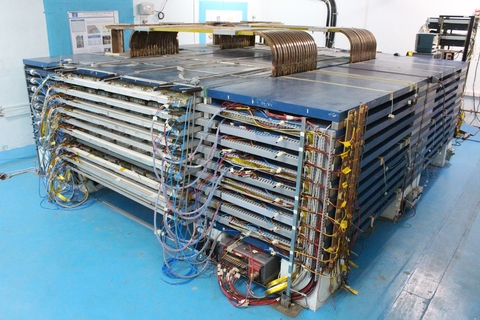
Figure 1: The mini-ICAL detector with 11 iron layers. The upper portion of copper coils and slots are clearly visible.

Figure 2: Schematic of top view of one mini-ICAL layer showing the plates A, B, C, D and the gaps 0–5.

3 Magnetic field measurements in the mini-ICAL

3.1 The Hall sensor probe and calibration

The procedure followed for the calibration of the Hall sensor PCB and estimation of error associated with the measured magnetic field is the same as described in Ref. [6], where measurements were presented for coil currents upto 500 A due to limitation of power supply. In the present paper, measurements are shown for currents upto 900 A, where saturation of magnetic field is expected.

Magnetic field measurements are done in the gaps 0–5 shown in Fig. 2 at coil current of 500 to 900 A in steps of 100 A using Hall probe PCB whose schematic is shown in Fig. 3. The probe has 16 CYSJ106C GaAs [8] Hall Effect Element sensors mounted on it and these are labeled from 0 to 15. Closer to the front end electronics is sensor no. 15 and the farther one is numbered as sensor no. 0. The probe is 75 cm in length and 3.8 cm in height. The Hall sensors are mounted 4.4 cm apart from each other and on alternate sides of it such that sensors with even numbers are on one side and sensors having odd sensor numbers are on the other side of the PCB. The thickness of Hall probe PCB becomes after mounting the sensors is 2.3 mm.

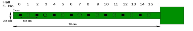
Figure 3: Hall probe PCB with 16 Hall sensors mounted on it

Before taking measurements of the field at mini-ICAL, the calibration and offset measurement of each sensor is done. A detailed description of the procedure can be found in Ref. [6]; the same procedure was used for the current set of measurements as well. To measure the offset, the Hall sensor is kept away from the mini-ICAL (any) magnetic field and the output voltage of each sensor is measured and plotted (see the left side of Fig. 4). The calibration of each sensor is done using an electromagnet designed and fabricated for the purpose of calibration. The field in the gap has been cross-calibrated using a precision Hall probe. The output Hall voltage of each sensor is noted for different magnetic field values. This is plotted and fitted with linear fit to extract the slope and intercept. A sample calibration curve for sensor number 8 is shown in the right side of Fig.-4.

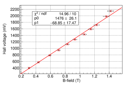
Figure 4: Left: Measurement of offset for all the sensors; Right: Calibration plot of sensor number 8.

The magnetic field is calculated from

$$B = \frac{V-V_{0}+V_{\epsilon}}{m}~{},$$

$$\delta{B} = \frac{B}{m}\sqrt{\frac{\Delta{V_{0}}^{2}}{B^{2}}+\Delta m^{2}}~{},$$ (3.1)

where $V$ is the measured Hall voltage, $V_{0}$ is the measured offset voltage (for each sensor), $m$ is the slope obtained from the calibration curve, and a small stray offset of V${}_{\epsilon}\lesssim 20$ mV was included to get agreement between the odd and even sets of sensors. Here the errors in the measurement is $\delta{B}$, which depends on the error in offset measurement, $\Delta{V_{0}}$ and the error in the slope from the calibration curve $\Delta m$. In Fig. 5 the magnetic field measurement in the gap-2 is shown for the coil current of 900 A. Here the sensor number 0 is nearest to the coil and sensor number 15 is nearest to the outer edge of the iron layer. The upper $x$-axis of Fig. 5 is labelled according to the actual distance of each sensor from the edge of the detector/layer.

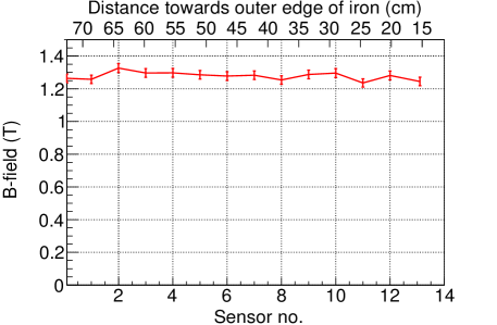
Figure 5: Sample magnetic field measurement in the gap-2 at 900 A coil current as obtained from the calibration and offsets discussed in the text

.

3.2 Magnetic field measurements in the top layer

The measured magnetic field is plotted as a function of the coil current, in steps of 100 A up to a maximum of 900 A, in Fig. 6 for gaps 0 and 4. The results for gaps 2,3,5, are similar to that for gap 0, and gaps 1 and 4 have similar behavior. It can be seen that in the gap-0 (length 800 mm), the magnetic field reaches saturation at 900 A while the magnetic field in the gap-4 (length 980 mm) is still in the linear region and approaching saturation. Also, the magnitude of the field is smaller for the horizontal gap 4 than for the vertical gap 0. This behavior is also seen in the simulations study, as we will see later.

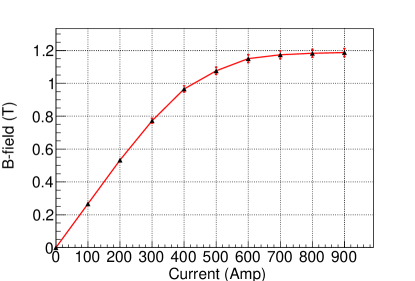
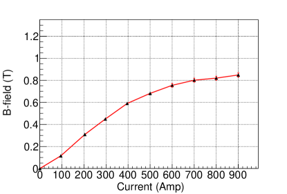
Figure 6: Measured magnetic field in the gaps 0 (left) and 4 (right) as a function of coil current in steps of 100 A.

The magnetic field as measured by the Hall probe sensors is plotted for the sample vertical gap-0 in Fig. 7 as a function of the distance from the detector edge, for coil currents, 500, 600, 700, 800 and 900 A. It can be seen that the field is more or less uniform across the gap, and increases with current, saturating just as shown in Fig. 6. A similar result is seen for the horizontal gap-4 as well, as also seen in Fig. 7. A small increase in the field is seen (for all values of coil current) towards the coil end of the gap.

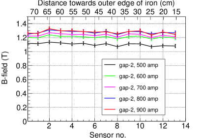
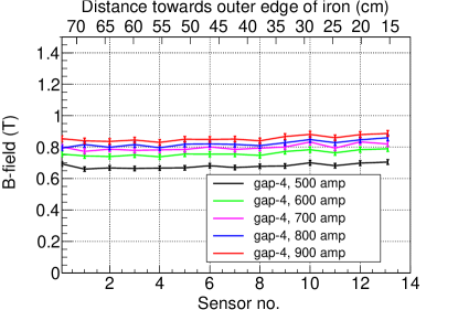
Figure 7: Measured magnetic field in the gaps 2 (left) and 4 (right) for coil currents from 500 to 900 A in steps of 100 A as a function of the distance from the detector edge.

Fig. 8 shows the same results, but for two different vertical gaps, 2 and 3, for a sample coil current of 900 A, which are expected to show similar behaviour. The RHS of the figure shows the same, but for horizontal gaps, 1 and 4 (gap-width shown in the Fig. 8 is averaged value, however gap - 1 is a bit wider near the edge and hence magnetic field near edge is less than the magnetic near the coil as can be seen Table. 2 and near the outer edge width of gap-4 is less than width near the coil therefore magnetic field is a bit more than magnetic field near the coil as can be seen in Table. 2). The difference in the magnitudes of the fields at these gaps is found to be [6] due to variations of the actual gaps from the design values. This has already been discussed for the measurement at 500 A in our earlier study and is visible for other values of coil current as well. Hence it is important to adjust for the gap widths. So, before going on with the description of the magnetic field measurements in mini-ICAL, we discuss details of the various gap widths.

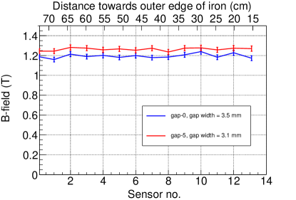
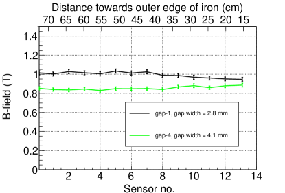
Figure 8: Measured magnetic field in the gaps 0,5 (left) and 1,4 (right) for coil current of 900 A as a function of the distance from the detector edge. These are expected to show similar behaviour as per the detector geometry. See text for more details.

3.3 Gap width measurements

It is observed that the width of the gaps which are introduced in the mini-ICAL to measure the magnetic field is different from the designed width. Gaps 0, 2, 3 and 5 were designed with width of 3 mm while gaps 1 and 4 were designed with widths of 4 mm. These gaps widths were slightly different from the design values due to assembly tolerances. In addition, it was found that the gap widths changed perceptibly when the coil current was turned on, due to torsional forces from the magnetic field. However, beyond a current of 500 A, there was no appreciable change found in the width as the current increased up to 900 A. These gap widths affect the magnetic field measured in the gaps as already discussed in Ref .[6], with gaps having smaller width showing higher magnetic field and vice versa. Hence an accurate measurement of the various gap widths is important in order to deduce the correct magnetic field.

These gap widths for gaps in the top layer of mini-ICAL were measured, on the top side, using (non-magnetic) brass vernier calipers and the values are shown in Table 2). Furthermore, it is observed that these gaps are varying in width, across their lengths, as can be seen from Table 2. It was shown in our earlier work that adjusting for the different gap widths results in matching of the magnetic field across similar gaps, viz., across gaps 0,2,3,5, and gaps 1,4. We will discuss this further once we have presented detailed studies of the magnetic field simulations.

Gap number $\to$	0	1	2	3	4	5
Measurements taken $\downarrow$	(in mm)
near coil	3.5	2.8	3.2	3.1	4.1	3.1
at middle	3.5	2.8	3.4	3.4	4.2	3.1
at outer edge of iron	3.5	2.9	3.2	3.6	3.9	3.0
Average value used	3.5	2.8	3.2	3.4	4.1	3.1

Table 2: Measured gap widths of the gaps 0–5 in the top layer of mini-ICAL, showing both the range of values as measured along their widths and their average, when the current is switched on. The measured widths are the same for currents in the range 500–900 A.

4 Magnetic field simulation using Infolytica MagNet software

A 3-D static magnetic field simulation is done using the Infolytica MagNet version 7.7 software [5] and the mini-ICAL geometry as one of the inputs. It uses finite element methods to calculate the magnetic field in the magnet volume. It divides the given geometry into small volume elements and solves the Maxwell’s equations in that part using approximate methods. The mini-ICAL geometry coded into the MagNet software is shown in Fig. 9. In what follows, an ideal mini-ICAL geometry is considered. After assembly of the mini-ICAL some changes in the dimensions are observed, such as variations in the actual gaps as described in Section 3.3, particularly after switching on the coil current, and their effect is discussed later.

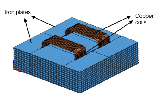
Figure 9: Schematic of the mini-ICAL geometry encoded in MagNet software.

We are interested in simulating the magnetic field over the entire mini-ICAL as well as, in particular, the $B$-field in the gaps. Since the mini-ICAL geometry is similar to ICAL, we shall display the simulated field along the diagonal ($x=y$ in mini-ICAL. As can be seen from Fig. 2, this line nicely captures the variation in $B$ from $B=0$ at $x=y=0$ mm at the bottom-left corner through the maximum value at the center, $x=y=2002$ mm to the top-right corner, $x=y=4004$ mm. It also traverses two 3 mm gaps between the C and D plates, which are regions of interest.

4.1 Inputs to the simulation

There are certain inputs that are required to perform the simulations. One important input is the $B$-$H$ curve which defines the behavior of the iron with respect to magnetization. Chemical composition of the steel used for the mini-ICAL is given in the Table 3, low carbon steel (from Essar Steel, Hazira, Gujarat) is used to build mini-ICAL and this shows a saturation magnetic field of 2.099 T; see Table 4. The other inputs for the simulations are the plate and coil geometry, mesh size and shape, and coil current.

Elements	C	Mn	Si	P	S	N	Al	Fe
%	0.015	0.368	0.188	0.012	0.008	0.005	0.001	Balance

Table 3: Chemical composition of the mini-ICAL steel.

Material	Low carbon steel
Young’s modulus	200 GPa
Density	7850 kg/m3
Poisson’s ratio	0.3
Yield strength	200 MPa (Min.)
Magnetic property	Knee point 1.5 T, H1T 300 A/m, H1.5T 900A/m

Table 4: Mechanical and magnetic properties of the steel used for mini-ICAL. Source: Essar Steel.

4.1.1 $B$-$H$ curve

The $B$-$H$ curve is a basic property of the material. It is used as an input parameter for the simulations and therefore it is important to measure it as accurately as possible. The $B$-$H$ curve is measured (with a commercial $B$-$H$ tracer) using a ring specimen with square cross section made from the same low carbon steel used in mini-ICAL. The Gaussmeter used in the measurement has an error of 1% in the 1 T magnetic field range, and is calibrated against a reference magnet [9]. The results of various data sets match with the reference input $B$-$H$ curve, shown in Fig. 10, which was used as an input for the MagNet 7.7 simulations.

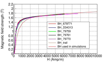
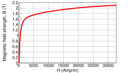
Figure 10: Left: Various measurements of the $B$-$H$ curve of different samples using a calibrated gaussmeter. Right: The $B$-$H$ curve used as an input in magnetic field simulations.

4.1.2 Mesh size and shape

It has been observed that mesh size plays a crucial role in the simulations. Simulations done using crude or default mesh (of size $\sim$ 300–400 mm) shows magnetic field values different than the simulations done using finer mesh (size $\sim$ 1–2 mm), especially where the field is changing rapidly. However it is observed that for even finer mesh size there is no significant change in magnetic field values while taking a much larger computation time and memory. Therefore optimization of the input mesh sizes is important.

Different mesh sizes are optimized for iron plates and gaps since iron plates ($\sim$ 1 m – 2 m) are of larger dimensions and gaps (dimensions $\sim$ 800 mm $\times$ 3 mm) are of small dimensions as compared to the iron plates. The mesh size for mini-ICAL geometry is optimized based on three factors—memory available in the system, simulation time and convergence in the magnetic field value. Since gap widths are smaller (3–4 mm), the mesh size used here was 2 mm. For the iron plates with larger dimensions (1000 mm–1200 mm), a mesh size of 10 mm was used.

To optimize the mesh size the magnitude of the field, $|B|$, is extracted for the complete layer and the fraction of area (%) having $|B|>1$ T is calculated with 900 A coil current and the change in the fraction is noted. It can be seen in Fig. 11 there is no significant change in the % fraction of area with magnetic field value $>1$ T below 2 mm of mesh size in the gap. Since the computation time for simulating the complete model is an acceptable 6–7 hours (on a desktop computer) for this mesh size in the gap, this was used in all subsequent simulations.

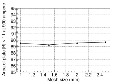
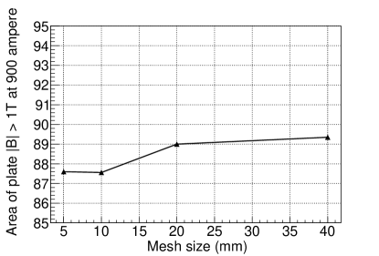
Figure 11: Fractional change in volume having $|B|>1$ T of a layer with change in mesh size in gaps (left) and iron plates (right).

A similar procedure was adopted to optimize the mesh size in the iron plates. From Fig. 11, it can be seen that the fraction of area (%) having $|B|>1$ T does not change for a mesh size below 10 mm while increasing the computation time and memory for smaller mesh sizes. Hence a mesh size of 10 mm was used for the iron plates in all simulations. Another metric for deciding the mesh size in the gap could be the convergence of the B-field there.

The change in magnetic field value with default and optimized mesh size is visible in Fig. 12. It is observed that the magnetic field value extracted along the diagonal line ($x=y$) of the mini-ICAL layer for the model simulated with optimized mesh (2 mm in the gap and 10 mm in the iron) is more smooth and symmetric as compared to the $B$-field values extracted from the model simulated with default mesh size (300–400 mm). In addition, the predictions for the $B$-field in the gap between C and D layers (at $x=y=1200$ mm and $x=y=2800$ mm) are very different between the two sets of simulations. Since we are going to validate the simulations by comparing the values of the $B$-field in the gap regions (in gaps 0–5) to the measured values, it is crucial to precisely determine the values in these gaps.

Also the model simulated with default mesh size shows magnetic field value which is larger than the model simulated with optimized mesh size. Therefore it can be seen that the optimization of mesh size is one of the important aspects of simulations. It may be mentioned that the shape of the mesh element used in the simulation has a tetrahedral shape.

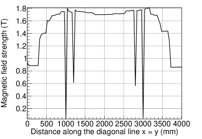
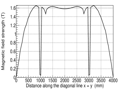
Figure 12: Magnetic field along the diagonal line of the top layer for 900 A coil current simulated with default mesh size $\sim 300$–400 mm (left) and with mesh size of 2 mm in the gaps and 10 mm in the iron plate (right). Note the $y$-axes are different in the two plots.

4.1.3 Coil Current

There are two sets of copper coils in mini-ICAL, each having 18 turns, and DC current is passed through these coils to magnetize the mini-ICAL magnet. The mini-ICAL magnetic field is simulated for 500, 600, 700, 800, 900 A of coil current. Since 500 A lies in the linear region of B-H curve it will give an insight into the magnetic field behavior in the linear region of B-H curve. Therefore simulations are performed for coil currents between 500 A and 900 A (near saturation of B-field) in steps of 100 A. Also, the results for 500 A current will be compared with the measurements made in the mini-ICAL detector currently functioning at Madurai.

4.2 Comparison between single layer and 11-layer model

Simulations are performed to study the change in magnetic field value for models of mini-ICAL having all the 11 layers and a single iron layer. This is done to find out if the $B$-field value does not change significantly; as a single layer or 3-layer model will require much less time and memory for the simulation. In Fig. 13 the $B$-field value along the diagonal line (see Fig. 2) is plotted to show the difference and it can be seen that in the middle plate i.e., D (central region between the two major dips) the $B$-field value is about 6% more for the model simulated with single iron layer and in the outer plates, the magnetic field value is about 3% more for the model simulated with 11 iron layers.

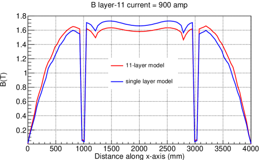
Figure 13: Comparison of magnetic field values along the diagonal line (see Fig. 2) for is plotted to show the 11-layer and single layer model.

From here it can be concluded that there is a significant difference between the magnetic field value calculated using a single layer and 11-layer model, although the origin of this difference is a bit subtle. It has to do with the counteracting effect of the field in the plates above and below the layer. Hence a 11-layer model was used for the simulation study although it requires more time and memory. A more detailed analysis of the variation in magnetic field due to the number and position of iron plates is given in Appendix A.

4.3 Simulated magnetic field in mini-ICAL

After simulations, a magnetic field map is generated for the layer of mini-ICAL (as generated for ICAL detector). The magnetic field map generated for one layer of mini-ICAL can be seen in Fig. 14.

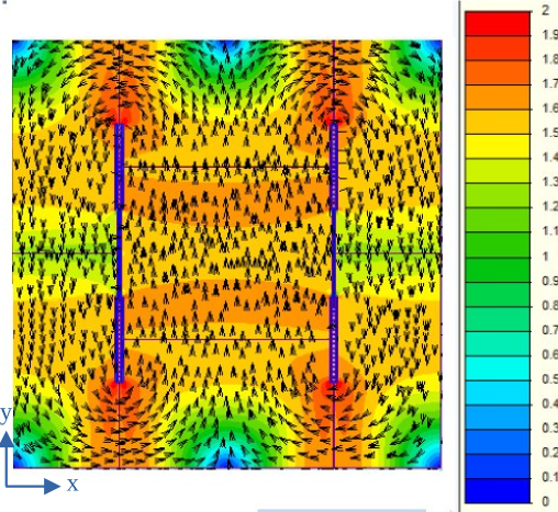
Figure 14: Magnetic field map simulated for the top layer of mini-ICAL for 900 A coil current.

This shows a close resemblance to the $B$-field map for the ICAL detector [4]. The $B$-field is maximum and uni-directional (in the $y$ direction) in the central region; in the side region (outside the coil slots, but in the central $y$ region from approximately 1000–3000 mm), it is in the opposite direction and a little less than in the central region and in the peripheral region (outside 1000–3000 mm in both $x$ and $y$ directions), it is varying in direction as well as magnitude. This also agrees with the measured magnetic field, where the field in the vertical slots (0,2,3,5) is much higher than in the horizontal slots 1,4, as seen from Fig. 7.

Data is also extracted for the magnetic field along the diagonal line (see Fig. 2) and in the gaps 0–5. The $B$-field value along the diagonal is shown in Fig. 15 for different values of the coil current. It can be seen that as the current approaches 900 A from 500 A the variation in the magnetic field values reduces due to the onset of saturation. It can be seen from Fig. 2 that the diagonal line crosses two coil slots and two gaps between the iron plates and hence gives a fair idea of the $B$-field over the entire detector. The four dips in the magnetic field along the diagonal line—two larger dips corresponding to the two coil slots (width - 80 mm) and two smaller ones corresponding to the gap between the iron plates C,D and D,C (which are approximately 3 mm in width) are thus explained.

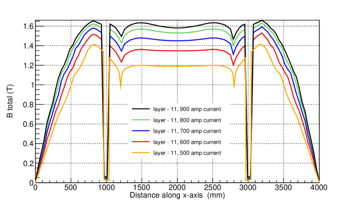
Figure 15: Magnetic field along the diagonal line (see Fig. 2) for the top layer of mini-ICAL at 500 A, 600 A, 700 A, 800 A and 900 A coil currents.

Fig. 16 (left) shows the magnetic field value along the line $y=500$ mm for $x=0$–4004 mm and the two dips are due to the gaps-2 and 3 (width - 3mm). In Fig. 16 (right) the simulated magnetic field is shown along the line $x=500$ mm, for $y=0$–4004 mm and the dip in the magnetic field is due to presence of air gap-1 (width - 4mm) as shown in Fig. 2. These are the gaps at which the magnetic field has been measured at mini-ICAL using Hall probes. Note that in the simulations, the field is symmetric with respect to gaps (0,3), (2,5) and (1,4).

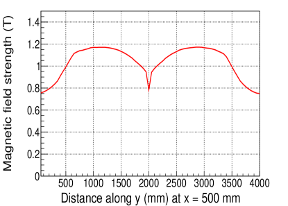
Figure 16: Left: Simulated magnetic field $|B|$ for (Left:) $y=500$ mm and for $x=0$–4004 mm, including gaps 2,3 and (Right:) $x=500$ mm and along $y=0$–4004 mm, including gap 1.

5 A detailed study of the simulated $B$-field in the gaps

In order to make a meaningful comparison between the measured and simulated magnetic fields, we need to determine the magnetic field in the gaps where the measurements have been made. The magnetic field values are extracted for all of the gaps where the magnetic field measurements at mini-ICAL have been done, to compare the simulated $B$-field with the measured field. It was already shown in Ref. [6] that although all the gaps — 0, 2, 3 and 5 are symmetric and ideally are of same width but the $|B|$ field values measured in these gaps are slightly different from each other which was due to variation in gap width. To study this, and account for these differences, simulations are performed by varying the gap widths.

5.1 Dependence of magnetic field on gap width

Since gaps 0, 2, 3, and 5 are identical by design (width 3 mm), and gaps 1 and 4 are also designed (width 4 mm) to be identical to each other, due to the symmetry of the geometry, we study the variation in the $B$-field due to changes in gap width for the representative gaps 0 and 1 only. The gap width for gap 0 is varied from 2.5 to 3.5 mm in steps of 0.25 mm and for gap 1 it is varied from 3 to 4 mm in steps of 0.25 mm and $B$-field is studied at these gaps. These are shown in Fig. 17 for gaps 0 (left figure) and 1 (right figure). On the left side, the magnetic field value is extracted for a fixed $x$ value corresponding to the position of the gap 0, with $y$ varying from $y=3200$–4000 mm, from inside the detector, to the outside edge. For gap 1, the $y$-value corresponds to the position of the gap 1, and the distance varies from $x=0$–980 mm from a point just outside the coil to the detector edge. Note that the gaps lengths are 800 mm for gap 0 and 980 mm for gap 1, since the Hall probe is 660 mm in length, it probes practically the entire length of the gaps 0, 2, 3, and 5 (barring 140 mm near the coil) while it cannot probe 320 mm also of the gaps 1 and 4 near the coil slots. Hence comparison between simulations and data is done, keeping this in mind. While the $B$-field is roughly constant over gap 1, it falls off with distance in gap 0.

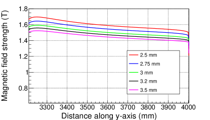
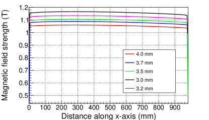
Figure 17: Simulated magnetic field values in gap 0 (left) and gap 1 (right) for varying gap widths; the larger distance values correspond to points closer to the detector edge.

Fig. 18 shows the change of $B$-field obtained due to variations in the gap width. Shown are the ratios of the results obtained by simulating the field for a given gap at an arbitrary position along the gap, to that obtained for a simulated gap with the design width (of 3 mm for gap 0 and 4 mm for gap 1). The results are robust and independent of the position chosen. From the $B$-field values extracted for the simulations with different gap widths, it is observed that the dependence on gap width can be parameterized by a linear fit. This can be used to calculate the $B$-field for any gap width by interpolating in the region of interest. It was also seen that either of the two fits, linear and parabolic, does not make much difference in the region of interest. Hence we shall assume a linear dependence on the gap width. The ratio corresponding to the actually measure gap width, as listed in Table 2, was found through interpolation of the data and fits determined in Fig. 18. This was used to determine the simulated $B$-field values corresponding to the actual gap values found in the measurement, by adjusting for the gap width.

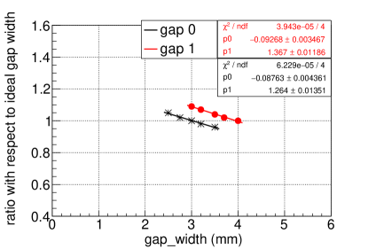
Figure 18: Scaling of magnetic field as a function of the gap width. Plotted here is the ratio of the $B$-field values obtained with a given gap width (as given along the $x$-axis) to the value of the $B$-field expected when simulating with the design gap width of 3 mm for gap 0 and 4 mm for gap 1. Also shown is a linear fit to the ratio, for use by interpolation to determine the simulated field at arbitrary gap values.

6 Comparison of simulated and measured magnetic fields

Recall that the gaps 0, 2, 3, and 5 all have a design width of 3 mm while gaps 1 and 4 have a design width of 4 mm; furthermore, as per the detector geometry, the gaps 0,2,3,5 are expected to show similar behaviour, and gaps 1,4 are expected to be similar; hence we consider these two sets separately.

We are now ready to compare the results of the simulation (for different coil currents) with the measurements of the $B$-field in the gaps discussed in the earlier section. In each case, we plot the ratio of the simulated to measured magnetic field with and without gap width corrections.

Coil current 500A

: If the measured magnetic field is compared with the simulations using an ideal gap value (i.e., 3 mm for gaps 0, 2, 3, 5 and 4 mm for gaps 1 and 4) and ratio of simulated magnetic field vs measured magnetic field is plotted, it can be seen from left of Figs. 19 (for coil current of 500 A),  20 (for coil current of 700 A) and  21 (for coil current of 500 A) that the results for gaps 2 and 5 are similar, indicating that their gap widths are similar, which is indeed the case as can be seen from Table 2. The measured magnetic field in the gap-3 is more than gap-0 as can be seen that gap width is more for gap-0 among gaps - 0, 2, 3 and 5. Also, since the ratios for gaps 0 and 3 are larger than for gaps 2, 5 we expect that the former have larger gaps than the latter, which is also true. Finally, we expect the ratios for gaps 1 and 4 to be similar but they are very different, again due to the considerable difference in their gap widths. Hence we see that the differences in measured values are significantly driven by the gap widths.

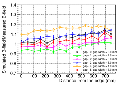
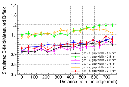
Figure 19: Left: Comparison of measured magnetic field with simulations done using design values of gap widths at the coil current of 500 A; Right: Comparison of measured magnetic field with simulations done with corrected gap widths (as per Table 2) at the coil current of 500 A. The agreement between various measured magnetic fields has improved but the ratios for the gaps-(1,4) and (0,2,3,5) are bunched together.

If the measured gap width (with gap width correction) is taken into account, the measured values of the magnetic field (and hence the simulated to measured ratios) are in agreement to within $\pm$ 5% of each other (see right side of Fig. 19) for the gaps 0, 2, 3 and 5 after gap correction and gaps 1 and 4 also. At 500 A coil current, the group of gaps-3 mm (0, 2, 3 and 5) are bunched together and 4 mm (1 and 4) are bunched together separately with a difference of $\sim$ 10%, indicating a mis-match between the simulations in the peripheral and side regions. This may happen because at coil current of 500 A, we are still in the linear region in the $B$–$H$ curve and any deviation in the B-H curve or an inhomogeneity in the bulk of the iron plate could be responsible for the deviation. This is particularly so since we have already seen, both in the measurement and the simulations, that the field around the horizontal gaps saturates at much higher currents that the vertical ones.

Coil current 700 A

: As the coil current is raised further towards saturation from 500 A to 700 A, the ratios of simulated to measured field for both the groups of gaps (0, 2, 3 and 5) and (1 and 4) begin to come closer together (see right side of Fig. 20). However, the ratio for both sets now exceeds unity for all gaps.

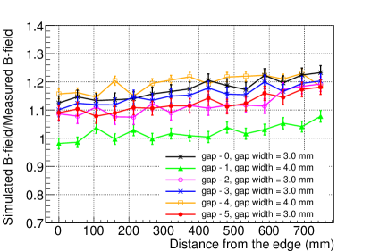
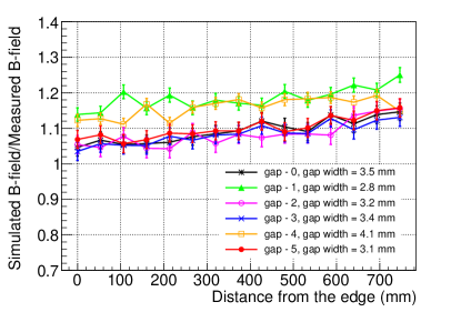
Figure 20: As in Fig. 19 for the coil current of 700 A; The ratio for both sets of gaps (0, 2, 3 and 5) and (1,4) now exceeds unity for all gaps.

Coil current 900 A

: This trend continues for coil current of 900 A: the ratios of simulated to measured field after gap-width correction begin to merge with each other (see right Fig. 21) for all six gaps, both the horizontal and vertical ones. Two points may be observed here: the simulated magnetic field is larger than the measured one for all gaps over their entire length. In addition, the ratio has an increasing slope, indicating that the field simulated inside the iron, near the coils is much larger than the measured one. This slope is especially perceptible for gaps 0,2,3,5, so that the ratio increases by 15% from the outer edge to the centre. The slope is much smaller for gaps 1,4 where the corresponding ratio increases by only 7%.

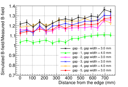
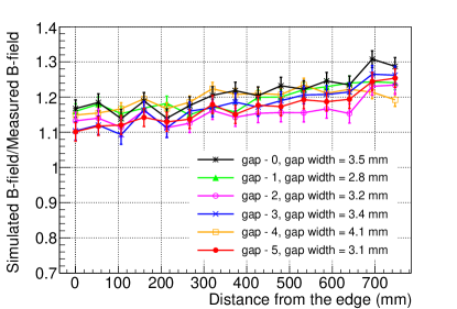
Figure 21: As in Fig. 19 for the coil current of 900 A; the ratio for both sets of gaps (0, 2, 3 and 5) and (1,4) exceeds unity for all gaps, but they are also converging to the same value for all six gaps.

7 Results and Discussion

A few remarks are in order. It is important to note that the field is fairly uniform over the entire gap width. Hence the thickness of the Hall probe, and whether the sensor was mounted on one side or other of the probe, does not change the measurement; otherwise it would be difficult to make a meaningful statement about the $B$-field in the gaps. In addition, while the field may differ substantially in the gaps depending on the width, the field in the iron itself remains practically the same throughout, for a given current, independent of the gap width (except at locations just adjacent to the gaps). Hence, once the field is measured in the gaps and the simulations result matched with these, it is not necessary to measure the fields at all gaps; the magnetic field map can be validated by just a few sample measurements. This is important, since it is not possible to measure the gap widths in all layers. Measuring the gap widths at the time of assembly is also not sufficient since they are different with and without the field due to torsional forces that bring the plates together when the current is switched on.

It is clear that the gap thickness measurement plays a crucial role while comparing the simulated and measured magnetic field. It was shown in Ref. [10] while studying the physics reach of ICAL, that while local random fluctuations of the magnetic field could be well-tolerated, systematic deviations from the true value (such as have been observed in this study) will significantly impact the results. For example, this may cause the fits to converge to a best-fit value different from the true/input value of the neutrino oscillation parameters such as $\sin^{2}\theta_{23}$ and $\Delta m^{2}_{32}$.

The present study shows that as the coil current approaches 900 A starting from 500 A, the simulated magnetic field is more than the measured magnetic field as can be seen from the right hand figures of Figs. 19, 20 and 21. In addition, while the magnetic field in the gaps 0, 2, 3, 5 increases from the edges towards the center of the detector, this increase is more pronounced in the simulations (especially for the vertical gaps) as compared to measurement, as discussed above. The origin of this discrepancy could be due to differences in the $B$-$H$ curve used in the simulations and the actual performance. Notice from Fig. 10 that different samples gave very similar $B$-$H$ curves. Hence, this is unlikely to be the source of this discrepancy. However, the plate manufacturing procedure that was used to cut the plates can generate heat-affected zones (HAZ) where the magnetic field properties can be significantly altered. Inhomogeneities in the bulk low-carbon steel plates and other material unaccounted for in the simulations (the simulations includes only the iron and copper coils and not the RPCs, electronics, etc) can also substantially degrade the magnetic field from the expected value. Minimizing the heat affected zone (HAZ) may help to improve the agreement with the simulations. However, the measurement can be used to normalize and calibrate the simulations in the short term, and guide other measurements that might help pinpoint the reasons for the discrepancy and help in a better understanding of the magnetic field in mini-ICAL. Although outside the scope of the present work, measurements on an appropriate prototype magnet using secondary beams of muons of known momentum would help validate the entire procedure.

Appendix A Simulations with different number of layers

As described in Section 4.2, the number of iron layers used in the model affects the simulated magnetic field. To confirm this, a study is done using models with different number of layers. Here, the dimensions of C and D plates is changed from 1200 $\times$ 2000 mm and 1962 $\times$ 1600 mm to 1200 $\times$ 3000 mm and 2962 $\times$ 1600 mm to check if the change in geometry makes any difference. This study is done for 900 A coil current with default mesh since it was done just to check the trend.

It is observed that the number of layers present in the model as well as their position with respect to each other makes a difference in the output magnetic field. We explain this as follows. We have considered 5 different models in addition to the standard 11-layer model. Two of them have 3 layers, placed at positions (1,6,11) or (5,6,7) of the 11-layer model. Two of them have 5 layers, placed at positions (1,3,6,9,11) or (2,4,6,8,10) of the 11-layer model. Finally, one model has just a single layer, placed in position 6 (centre) of the 11-layer model.

In Fig. 22 the magnetic field value along the diagonal line is shown for the middle layer (layer-6) for all 6 models considered. It can be seen that the magnetic field in this central layer is maximum for the single layer model and minimum for the 11-layer model. As 3 or 5 layers are added, the field decreases from the 1-layer model and is intermediate between the 1-layer and 11-layer models. However, the relative placement of the layers also matters: the field in the central module is always smaller either if there are more layers (2,4,6,8,10) or if the adjacent layers are closer to the central layer (5,6,7). Hence the 5-layer model (1,3,6,9,11) shows a larger magnetic field in layer-6 than the 5 layer model (2,4,6,8,10) where the layers adjoining the central one are closer. Similarly, the 3-layer model (1,6,11) with very distant neighbours has a larger magnetic field in layer 6 than the 3-layer model (5,6,7) with closely adjacent layers. Clearly the magnetic field in a layer depends on the number of adjoining layers as well as their relative distances from that layer. Finally, it may be noted that the behaviour is roughly inverted in the region outside the coil slots.

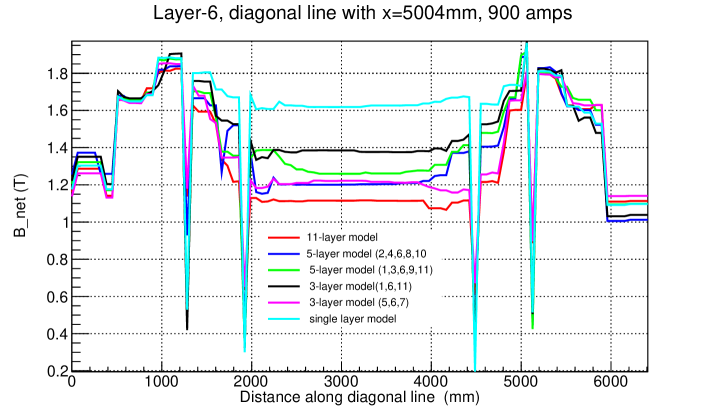
Figure 22: Magnetic field along the diagonal line $x=y$ in the central layer for models with different number of layers and different relative positions of the layers, as shown.

References

- [1] Shakeel Ahmed et al., ICAL collab., INO White Paper, Pramana 88 (2017) 5, 79; doi 10.1007/s12043-017-1373-4, [arXiv: 1505.07380 [physics.ins-det]].
- [2] D. Indumathi and M. V. N. Murthy, “A question of hierarchy: matter effects with atmospheric neutrinos and anti-neutrinos", 10.1103, Phys. Rev, D 71 013001, arXiv: hep-ph/0407336 [hep-ph].
- [3] S. Agostinelli et al., Geant4, a simulation toolkit, Nucl. Instr. Meth. in Physics Res. A 506 (2003), 250.
- [4] Shiba P Behera et al., IEEE Transactions on Magnetics 51, 7300409 (2014).
- [5] Infolytica Corp., Electromagnetic field simulation software, http://www.infolytica.com/en/products/magnet/.
- [6] Khindri Honey et al., Magnetic field measurements on the mini-ICAL detector using Hall probes, JINST 17 (2022) T10006, doi 10.1088/1748-0221/17/10/T10006.
- [7] Honey et al., Magnetic Field Simulations and Measurements on Mini-ICAL In: Mohanty, B., Swain, S.K., Singh, R., Kashyap, V.K.S. (eds) Proceedings of the XXIV DAE-BRNS High Energy Physics Symposium, Jatni, India. Springer Proceedings in Physics, 277, 2022, Springer, Singapore. https://doi.org/10.1007/978-981-19-2354-8_143; Honey Khindri et al., Simulations studies of the magnetic field in the mini-ICAL prototype using MAGNET software, 2023, in preparation.
- [8] Data sheet CYSJ106C, ChenYang Technologies GmbH and Co. KG, Version 2 Released in May 2016.
- [9] Digital gaussmeter, Ferrites India, www.ferrites-india.com; calibration certificate traceable to NPL, New Delhi.
- [10] Khindri, Honey, Indumathi, D. and Mohan, Lakshmi S., Impact of errors in the magnetic field measurement on the precision determination of neutrino oscillation parameters at the proposed ICAL detector at INO, arXiv:2305.07291 [hep-ph] (2023).