Stability control for USVs with SINDY-based online dynamic model update

Abstract

Unmanned Surface Vehicles (USVs) play a pivotal role in various applications, including surface rescue, commercial transactions, scientific exploration, water rescue, and military operations. The effective control of high-speed unmanned surface boats stands as a critical aspect within the overall USV system, particularly in challenging environments marked by complex surface obstacles and dynamic conditions, such as time-varying surges, non-directional forces, and unpredictable winds. In this paper, we propose a data-driven control method based on Koopman theory. This involves constructing a high-dimensional linear model by mapping a low-dimensional nonlinear model to a higher-dimensional linear space through data identification. The observable USVs dynamical system is dynamically reconstructed using online error learning. To enhance tracking control accuracy, we utilize a Constructive Lyapunov Function (CLF)-Control Barrier Function (CBF)-Quadratic Programming (QP) approach to regulate the high-dimensional linear dynamical system obtained through identification. This approach facilitates error compensation, thereby achieving more precise tracking control.

1 Introduction

With the widespread integration of automation and intelligence across various industries and the rapid advancement of unmanned and intelligent surface ships today Liu et al. (2016), the precise planning and control of high-speed Unmanned Surface Vessels (USVs) have become increasingly crucial. This significance is particularly pronounced in complex scenarios featuring time-varying characteristics that are challenging to accurately model. Such scenarios include the effects of time-varying winds, fluctuating water currents, surge disturbances, and other factors. Despite the difficulty in achieving high-accuracy modeling of USVs, it is essential not only to consider the influence of the vessel’s own dynamics but also to accurately measure and model the time-varying complexities of the environment. Even with high-precision ship dynamics models and intricate environmental models, the computational complexity becomes overwhelming when dealing with the ultra-high dimensional nonlinear model necessary for accurate planning, precise tracking, and control. Traditional numerical tools Makaroff et al. (1995) face challenges meeting the real-time regulation and control requirements of USVs due to the computational demands associated with high-dimensional modeling. Given these challenges, there is an urgent need for a novel modeling and control method that accurately captures the nuances of ships and vessels while ensuring that the computational solution complexity remains manageable and does not increase excessively.

To address these challenges, this paper proposes a data-driven approach based on the Koopman operator Koopman (1931) for real-time modeling of surface high-speed unmanned vessels. The control solutions of these vessels are derived through a quadratic programming problem (QP), constructed using the Control Lyapunov Function (CLF) and the Control Barrier Function (CBF). Specifically, we perform online data collection of the ship’s observable state and control quantities, encompassing the geodetic coordinates of the ship’s position ($x$, $y$), attitude angles (roll angle $R$, pitch angle $P$, yaw angle $Y$), velocity components ($u$, $v$, $r$), and the magnitudes of the three-axis moments generated by paddles and rudders ($\tau_{u},\tau_{v},\tau_{r}$). These data are then utilized for sparse identification Kaiser et al. (2018) of the nonlinear dynamics, resulting in high-dimensional linear approximate dynamical equations. The proposed control strategy involves tracking and regulating trajectories obtained from the original planning using the constructed CLF-CBF-QP. To streamline the real-time computation of the sparse discrimination system, an error threshold approach is introduced. This involves comparing the error relationship between the actual control results and the trajectory planning results. When the difference exceeds a certain threshold, the latest observed state quantities in the time domain are employed to re-evaluate the sparse discrimination of the system. Consequently, the parameters of the original system model are updated, enabling accurate real-time modeling of complex time-varying environment models. The high-dimensional linear real-time approximate dynamics model, acquired through sparse dynamics identification, is formulated in affine form. This allows for the convenient solution of the optimal control problem to obtain time-varying control quantities for the system.

The conclusive simulation experiments demonstrate a notable enhancement in control accuracy when compared to the control method lacking system identification. The integration of the error domain identification system proves effective in achieving comprehensive identification of the entire system, with lower overall system load requirements. This eliminates the necessity for real-time system identification and parameter updates.

The structure of this article is organized as follows. Section 1 provides a review of recent advancements in Unmanned Surface Vehicles (USVs) control and system identification, highlighting our primary contributions in this study. Section 2 predominantly elucidates the core theories of the Koopman operator, Control Lyapunov function, Control Barrier function, and other pertinent theoretical foundations. In Section 3, we expound on the principal model and construction methodology employed in our work. Section 4 is dedicated to the execution of simulation experiments, evaluating our proposed model and architecture. Section 5 summarizes the key findings of this paper and engages in a discussion on future prospects and potential avenues for further research.

1.1 Related work

To achieve fast and precise control of Unmanned Surface Vehicles (USVs), significant efforts have been devoted to the exploration of state-of-the-art control techniques in this field. In recent years, notable developments have emerged in ship control. Du et al. Du et al. (2022) demonstrated improved control outcomes through the application of adaptive reinforcement learning for USVs. However, there is a need for more in-depth research on reinforcement learning’s generalization, training time cost, and interpretability. Dong et al. Dong et al. (2015) utilized Backstepping Control (BC) to track USVs, employing a nonlinear controller design. Other control strategies, including Linear Quadratic Regulator (LQR) Yazdanpanah et al. (2013), Reference Adaptive Control (RAC) Baek and Woo (2022), and sliding mode control (SMC) Gonzalez-Garcia and Castañeda (2021), have been investigated for achieving trajectory tracking control in USVs. Wang et al. Wang et al. (2022) proposed an integrated planning and control framework for USV navigation, employing a combination of the artificial potential field method and model predictive control. This approach enables fast maneuvering and precise control in highly complex environments. However, its inherent dynamics model remains invariant, posing challenges in achieving optimal maneuvering in systems experiencing time-varying conditions, such as extreme winds and waves. Furthermore, extensive research on ship control has been conducted by Li Li et al. (2008), Annamalai Annamalai et al. (2014), and Oh Oh and Sun (2010), who constructed Model Predictive Control (MPC) models for ships, providing comprehensive insights into control methodologies based on the model predictive control approach.

While Model Predictive Control (MPC) offers high accuracy and trajectory tracking precision in the control of surface vessels like ships, it introduces challenges. MPC considers the tracking situation in the future time domain, thereby increasing the length and complexity of control. The incorporation of nonlinearization constraints on obstacles and the ship’s model poses difficulties in ensuring the efficiency of the optimal problem, particularly in extreme and high-speed scenarios. Consequently, effective optimal control becomes challenging, and MPC encounters limitations in addressing these situations. To address some of these challenges, Nonlinear Model Predictive Control (NMPC) Guerreiro et al. (2014); Sutton et al. (2011) has been proposed. NMPC exhibits higher control accuracy compared to the linearized model for Unmanned Surface Vehicles (USVs). However, it comes with a trade-off, as it significantly impacts the real-time requirements of the solution, posing challenges in meeting stringent real-time control demands.

The majority of the aforementioned methods rely on modeling or approximating existing ship models, with ship control achieved through the design of controllers adhering to Lyapunov stability principles Liu et al. (2016). While these methods enhance ship control accuracy to a certain extent and exhibit a degree of robustness, they encounter challenges when confronted with highly complex environmental changes. Situations where external factors like water flow and wind direction experience sudden and dramatic shifts, and these environmental conditions persistently evolve over time pose difficulties for the effectiveness of the mentioned control methods in maintaining optimal ship control.

In recent years, data identification and data-driven methods have gained widespread application in identifying and updating parameters for dynamic systems, including vehicles Lee et al. (2019), aircraft Cao et al. (2017), and chaotic systems Brunton et al. (2017). By observing and collecting data from dynamic systems, data analysis and prediction allow for compensation of the original ground dynamics system. This approach not only mitigates inaccuracies in system modeling but also enhances control accuracy. For instance, the Gaussian process regression method has been employed to identify and compensate online data for the dynamic system of vehicles Lee et al. (2019). This application proves effective in achieving better control of the vehicle, especially under challenging working conditions.

Parameter identification for the dynamics of Unmanned Surface Vehicles (USVs), vehicles, quadrotors, and similar systems significantly influences the accuracy of control actuators. Typically, two approaches are employed for identifying the parameter model of these actuators: offline identification and online identification. Various data from the actuators are collected by sensors on the aircraft, and more precise dynamic model parameters are obtained using methods such as frequency domain identification Selvam et al. (2005), time domain identification Mišković et al. (2011), artificial neural networks Rajesh and Bhattacharyya (2008), among others. However, offline identification involves a large overall scale of parameters to be identified, and various noises are introduced throughout the identification process. This makes it challenging to update controller parameters in real-time. Online identification methods, such as the feedback-forward compensation method Zhang et al. (2011) and recurrent neural networks Annamalai et al. (2014), also have some drawbacks, including poor interpretability.

While the modeling, identification, and regression of physical world action models obtained through artificial neural networks, deep neural networks, and reinforcement learning have been extensively explored and have demonstrated exceptional accuracy, particularly in domains like speech, vision, and text, their performance often surpassing traditional algorithms, it’s crucial to note a significant drawback. The models obtained through these approaches often function as black box models, lacking in robust physical interpretability. In contexts such as the identification of physical world models, interpretability and parsimony are of utmost importance Bongard and Lipson (2007). This holds true for the control of nonlinear systems Zhang et al. (2020), where understanding the underlying mechanisms is essential. Without adequate interpretability, accurately tracing and addressing real-world issues becomes challenging.

1.2 Our contributions

The primary contribution of this paper lies in introducing a data-driven framework for online Unmanned Surface Vehicles (USVs) dynamic parameter identification and control updates. This framework enables rapid and accurate regression and reconstruction of time-varying USVs dynamic parameters, as well as time-varying environmental models, including wind speed, wind direction, water flow, and more. Additionally, the control model is updated with minimal computational load. The final stage involves tracking and controlling USVs through the formulated Constructive Lyapunov Function (CLF)-Control Barrier Function (CBF)-Quadratic Programming (QP) problem. The specific contributions of this work are outlined below:

1. This paper introduces a novel online data compensation and dynamic parameter update control framework for Unmanned Surface Vehicles (USVs) based on sparse dynamics identification. Experimental results demonstrate excellent performance of regressing the observed parameters of USVs collected by sensors, yielding a high-dimensional linear approximate dynamic model.

2. The proposed framework employs a real-time observation data collection method, incorporating an error threshold to mitigate the complexity and computational load associated with the entire dynamics identification process.

3. By utilizing the high-dimensional linear approximate dynamic model instead of a low-dimensional nonlinear simplified dynamic model, the complexity of the control solution is reduced, leading to an enhancement in real-time control performance.

4. Real-time online data collection and parameter updates are employed to dynamically update the USVs control model through Constructive Lyapunov Function (CLF)-Control Barrier Function (CBF)-Quadratic Programming (QP). This ensures accurate and reliable tracking in real-time.

2 Preliminaries

In this section, we will present the sparse dynamic regression method based on the Koopman operator that is employed in this paper. Additionally, we will introduce the concepts of Control Lyapunov Function (CLF) and Control Barrier Function (CBF).

2.1 Koopman operator

The Koopman operator $\mathcal{K}$ was introduced by Koopman B.O. in 1931 Koopman (1931). This operator transforms finite-dimensional nonlinear problems into linear problems in infinite dimensions, providing an approximate solution to the original nonlinear control problem by addressing the transformed linear control problem. However, direct solutions to infinite-dimensional linear problems pose challenges. In recent years, as big data analysis has evolved, the approximation of infinite-dimensional linear problems through the combination of finite-dimensional linear functions has gained attention. This resurgence has brought the $\mathcal{K}$ operator back into focus. The core and challenge of Koopman construction involve elevating the dimension matrix (or $\mathcal{K}$ operator matrix) from the original nonlinear observations to the high-dimensional linear observation matrix. Commonly used methods for this purpose include Dynamic Mode Decomposition (DMD) Schmid (2010), Extending Dynamic Mode Decomposition (EDMD) Williams et al. (2015), Principal Component Analysis (PCA) Wold et al. (1987), Proper Orthogonal Decomposition (POD) Berkooz et al. (1993), and more. Moreover, recent research has explored finding the optimal $\mathcal{K}$ operator using methods such as neural networks Yeung et al. (2019); Xiao et al. (2022), representing a current research hotspot.

To commence, let us consider a discrete-time nonlinear dynamic system Brunton and Kutz (2022) evolving as:

$$x_{k+1}\,\,=\,\,f\left(x_{k}\right),\,\,x\in\mathcal{M}$$ (1)

Where $x_{k}$ represents the observable or unobservable states of the system. Furthermore, we define an observation function.

$$y_{k}\,\,=\,\,g\left(x_{k}\right)$$ (2)

where, $y_{k}\in\mathcal{N}$, and the $g\left(x\right)\in\mathbb{K}:\mathcal{M}\rightarrow\mathcal{N}$, these observations may be physical quantities with some specific meaning, such as the position, velocity, and so on of the USVs and $\mathbb{K}$ is a function space. On this paper, we assume that $\mathbb{K}$ is the $L^{2}$ space, and the Koopman operator, $\mathcal{K}:\mathbb{K}\rightarrow\mathbb{K}$, which can be defined as:

$$\left[\mathcal{K}g\right]\left(x_{k}\right)\,\,=\,\,g\left(f\left(x\right)\right)$$ (3)

From 3, we observe that the Koopman operator maps elements from the set $\mathbb{K}$ to the same set $\mathbb{K}$. Therefore, we can omit the mapping function $f(\cdot)$ between two time steps, and Eq. 3 can be expressed as:

$$\left[\mathcal{K}g\right]\left(x_{k}\right)=g\left(F\left(x_{k}\right)\right)=g\left(x_{k+1}\right)$$ (4)

Utilizing the $\mathcal{K}$ operator and the current state in the time domain, the state of the system at the next time can be inferred. Ultimately, the observable system states can be extended to a multi-state superposition and multi-step deduction to reconstruct the system.

2.2 Sparse identification of nonlinear dynamics with control

The use of machine learning for identifying nonlinear dynamic systems is gaining popularity. However, more accurate regression models based on machine learning often suffer from drawbacks such as poor interpretability and slow regression. Sparse dynamic regression methods Chen et al. (2014); Xu et al. (2014) for identifying dynamic models can effectively mitigate these issues.

Drawing inspiration from the overall architecture of SINDy Kaiser et al. (2018), the nonlinear dynamical system in the discrete form of Eq. 1 can be reformulated into the following continuous form:

$$\frac{\mathrm{d}}{\mathrm{dt}}x=\dot{x}=f\left(x,u\right),\,\,x\left(0\right)=x_{0}$$ (5)

The sparse identification of nonlinear dynamic systems Kaiser et al. (2018) involves collecting all observations of the system. Through sparse regression, the method identifies the terms most closely related to the quantized system state, constructing an approximate high-dimensional linear model of the system. The candidate invariant subspace library $\mathcal{Q}(X,U)$ is generated by linear or nonlinear combinations of the original state and control variables. The iterative least squares method is then employed to approximate the regression of the sequence of derivatives $\dot{X}$ of the original state variable. A differential equation matrix is constructed based on observable data, ultimately yielding a high-dimensional linear approximation of the original dynamic model.

The candidate invariant subspace library $\mathcal{Q}(X,U)$ can be constructed by measuring $T$ snapshots of the USVs’ system states $X$ and control values $U$ in real-world actions.

$$X\,\,=\,\,\left[x_{1},x_{2},\cdots,x_{T}\right]\,\,\mathrm{and}\,\,U\,\,=\,\,\left[u_{1},u_{2},\cdots,u_{T}\right]$$ (6)

Then, the candidate invariant subspace library $Q$ can be constructed as follows,

$$\mathcal{Q}\left(X,U\right)=\left[1X\,\,U\left(X\otimes X\right)\,\,\cdots\left(X\otimes U\right)\cdots\sin\left(X\right)\cos\left(X\right)\cdots\right]$$ (7)

where,$X\otimes U$ represents all the product combinations of the $x$ and $u$.

The system in Eq. 5 can thus be written as:

$$\dot{X}^{T}=\mathcal{Q}\left(X,U\right)\varPsi$$ (8)

The derivative of the state $X$ with respect to time $t$, denoted as $\dot{X}=,,\left[\dot{x}_{1},\dot{x}_{2},\ldots,,\dot{x}_{T}\right]$, if not directly measurable, can be obtained through numerical differentiation methods, such as fourth-order central difference or approximation using the total variation regularized derivative Rudin et al. (1992); Chartrand (2011). In practice, the high-dimensional representations of most dynamical systems exhibit only a few changing entries, implying that the coefficient matrix $\mathcal{Q}$ is sparse. Consequently, sparse matrix regression can be employed, requiring fewer nonlinear coefficients in the regression model.

$$\psi_{k}=\underset{\hat{\psi}_{k}}{\mathrm{arg}\min}\frac{1}{2}\left\|\dot{X}_{k}-\mathcal{Q}\left(X,U\right)\hat{\psi}_{k}\right\|_{2}^{2}+\sigma\left\|\hat{\psi}_{k}\right\|_{1}$$ (9)

Here, $\dot{X}_{k}$ represents the $k$-th row of $\dot{X}$, $\psi_{k}$ is the $k$-th row of $\Psi$, $\sigma$ is the sparse hyperparameter, which tunes the threshold of iterative sparse regression. The term $\left|\cdot\right|_{1}$ promotes the sparsity of the coefficient vector $\psi_{k}$. To approximate the solution of the optimization problem, methods such as sequential threshold least squares Brunton et al. (2016) or LASSO Tibshirani (1996) can be employed.

2.3 Control Lyapunov Function

For the general nonlinear controlled system Eq. 5 or the approximated system by SINDy in Eq. 8, we also could rewrite as a time-invariant control affine system:

$$\dot{x}=f(x)+g(x)u$$ (10)

where $f:\mathbb{R}^{n}\rightarrow\mathbb{R}^{n}$ and $g:\mathbb{R}^{n}\rightarrow\mathbb{R}^{n\times m}$ are Lipschitz continuous in $x$, and we assume that $x_{e}\equiv 0$ is an equilibrium point.

If there exists a constant $c>0$, and $V\left(x\right):\mathbb{R}^{n}\rightarrow\mathbb{R}$ is a continuously differential function such that:

1. $\varOmega_{c}:=\left\{x\in\mathbb{R}^{n}:V\left(x\right)\leqslant c\right\}$, which bounded the sublevel set $V(x)$.

2. $V(x)>0$ for all $s\in\mathbb{R}^{n}\setminus\left\{x_{e}\right\}$, and $V(x_{e})=0$.

3. $\underset{\mathrm{x}\in\mathrm{U}}{\mathrm{inf}}\dot{V}\left(x,u\right)<0$ for all $x\in\varOmega_{c}\setminus\left\{x_{e}\right\}$.

That the $V(x)$ is called a local control Lyapunov Function and $\varOmega_{c}$ is a region of attraction (ROA), i.e. every state in $\varOmega_{c}$ is asymptotically stable to $x_{e}$.

The derivative of $V(x)$ along the dynamics is affine in $u$:

$$\dot{V}\left(x,u\right) =\nabla V\left(x\right)\dot{x}$$ (11)

$$=\nabla V\left(x\right)f\left(x\right)+\nabla V\left(x\right)g\left(x\right)u$$

$$=\mathcal{L}_{f}V\left(x\right)+\mathcal{L}_{g}V\left(x\right)u$$

where, $\mathcal{L}_{f}V(x):=\nabla V(x)\cdot f(x)$ is the Lie derivative operator.

If the $V(x)$ is a continuously, differentiable, positive definite and radially unbounded function, $\lambda>0$ is a constant term, that satisfy the following,

$$\underset{u\in U}{\mathrm{inf}}\dot{V}\left(x,u\right)+\lambda V\left(x\right)\leqslant 0$$ (12)

The function $V(x)$ serves as an Exponentially Stabilizing Control Lyapunov Function (ES-CLF), indicating that for any $x\in\mathbb{R}^{n}$, it is exponentially stabilizable to $x_{e}$ Ames (2014). Here, $\lambda$ represents the decay rate of the upper bound of $V(x)$.

2.4 Control Barrier Function

Definition 1

(extended class $\mathcal{K}_{\infty}$). A continues function $\beta:\left(-b,a\right)\rightarrow\mathbb{R}$ for $a,b>0$ is called extended class $\mathcal{K}_{\infty}$ function if:

$\bullet$ $\beta(\cdot)$ is strictly increasing;

$\bullet$ $\beta(\cdot)$ is s.t. $\beta(0)=0$;

$\bullet$ $\underset{r\rightarrow-\infty}{\lim}\beta\left(r\right)=-\infty,\underset{r\rightarrow\infty}{\lim}\beta\left(r\right)=\infty$;

Definition 2

(Forward invariance)Chai and Sanfelice (2018). For a set $\mathcal{S}\subset\mathbb{R}$ is called forward invariant for system 10, if $z_{0}\in\mathcal{S}\,\,$ and $z\left(t,z_{0}\right)\in\mathcal{S},\forall t\geqslant 0$.

Consider a set $\mathcal{S}$, which defined as the $zero-superlevel\,\,set$ of a continuously differentiable function $\mathcal{B}:\mathcal{D}\subset\mathbb{R}^{n}\rightarrow\mathbb{R}$, yielding:

$$\mathcal{S} =\left\{z\in\mathcal{D}\subset\mathbb{R}^{n}:\mathcal{B}(z)\geq 0\right\}$$ (13)

$$\partial(\mathcal{S}) =\left\{z\in\mathcal{D}\subset\mathbb{R}^{n}:\mathcal{B}(z)=0\right\}$$

$$\text{Int}(\mathcal{S}) =\left\{z\in\mathcal{D}\subset\mathbb{R}^{n}:\mathcal{B}(z)>0\right\}$$

We called the $\mathcal{S}$ as the safe set.

The time derivative of $\mathcal{B}(z)$ along the state trajectories is

$$\frac{d\mathcal{B}\left(z\right)}{dt}=\nabla\mathcal{B}\left(z\right)\dot{z}=\frac{\partial\mathcal{B}\left(z\right)}{\partial z}\dot{z}=\frac{\partial\mathcal{B}\left(z\right)}{\partial z}\left(f\left(z\right)+g\left(z\right)u\right)$$

and using the Lie derivative as the formation

$$\frac{d\mathcal{B}\left(z\right)}{dt}=\mathcal{L}_{f}\mathcal{B}\left(z\right)+\mathcal{L}_{g}\mathcal{B}\left(z\right)u$$

Definition 3

(Control barrier functions(CBFs)). For a continuous and differential function $\mathcal{B}(z)$, and a set $\mathcal{D}$, if there exists an extended class $\mathcal{K}_{\infty}$ function $\alpha$ such that

$$\underset{u\in U}{sup}\left\{\mathcal{L}_{f}\mathcal{B}\left(z\right)+\mathcal{L}_{g}\mathcal{B}\left(z\right)u+\beta\left(\mathcal{B}\left(z\right)\right)\geqslant 0\right\}$$

for all $z\in\mathcal{S}$.

Where $\mathcal{S}\subset\mathcal{D}\subset\mathbb{R}^{n}$, and $\mathcal{S}$ satisfied the equation 13 for system 10.

We refer to function $\mathcal{B}(\cdot)$ as the control barrier function of system 10.

3 Problem formulation

In this part, we will introduce the USVs dynamic model, the framework of the all the system that combine the online-SINDy, parameters update and the CLF-CBF-QP controller.

3.1 USVs Model

In this paper, we focus on the motion of Unmanned Surface Vehicles (USVs) with three degrees of freedom on the water surface, neglecting the motion with three degrees of freedom, including pitch, roll, and heeling. Fig. 1 illustrates the inertial coordinate system and the ship body coordinate system. The typical kinematic model for USVs, without the presence of disturbances, can be expressed as:

$$\dot{\eta}=R\left(\varphi\right)\nu$$ (14)

Where, $\eta=[x,y,\varphi]^{T}$ denotes the vector of the position and orientation in the coordinates of the earth-fixed reference frame, $\nu\,\,=\,\,\left[u\,\,v\,\,r\right]^{T}$ denote the linear velocity and the yaw angular velocity moving in the x and y directions in the hull coordinate system, respectively. And

$$R\left(\varphi\right)=\left[\begin{matrix}\cos\varphi&-\sin\varphi&0\\ \sin\varphi&\cos\varphi&0\\ 0&0&1\\ \end{matrix}\right]$$

According to the hydrodynamic modelFosseN (2021) and Newton-Euler formula, the nonlinear dynamic model of USVs can be expressed as follows,

$$M_{0}\dot{V}+C_{0}(V)V+D_{0}\left(V\right)V=\tau$$ (15)

where,

$$M_{0}=M_{A}+M_{RB}$$

$$C_{0}\left(V\right)=C_{A}\left(V\right)+C_{RB}\left(V\right)$$

$$D_{0}\left(V\right)=D\left(V\right)$$

and the physical meanings of symbols in Eq. 15 are outlined in table. 1. Combine the Eq.14 and Eq. 15, the nonlinear dynamic model of the USVs can be expressed as follows,

$$\dot{x} =u\cos\varphi-v\sin\varphi$$ (16)

$$\dot{y} =u\sin\varphi+v\cos\varphi$$

$$\dot{\varphi} =r$$

$$\dot{V} =M_{0}^{-1}\left(\tau-C_{0}\left(V\right)V-D_{0}V\right)$$

The detailed content of each parameter matrix is beyond the main scope discussed in this paper, and we will not delve into them here. For more information, refer to the details provided in reference Liu et al. (2016).

Table 1: Nomenclature of USVs parameters

Symbols	Explanation
$M_{0}$	Inertia matrix
$M_{A}$	Additional mass matrix
$M_{RB}$	Rigid body inertia matrix
$C_{0}(V)$	Coriolis and centripetal matrix
$D_{0}(V)$	Hydrodynamic damping matrix
$C_{A}(V)$	Hydrodynamic Coriolis and centripetal matrix
$C_{RB}(V)$	Rigid body Coriolis and centripetal matrix
$\tau$	Control inputs($\tau=[\tau_{u}\,\,\tau_{v}\,\,\tau_{r}]$)

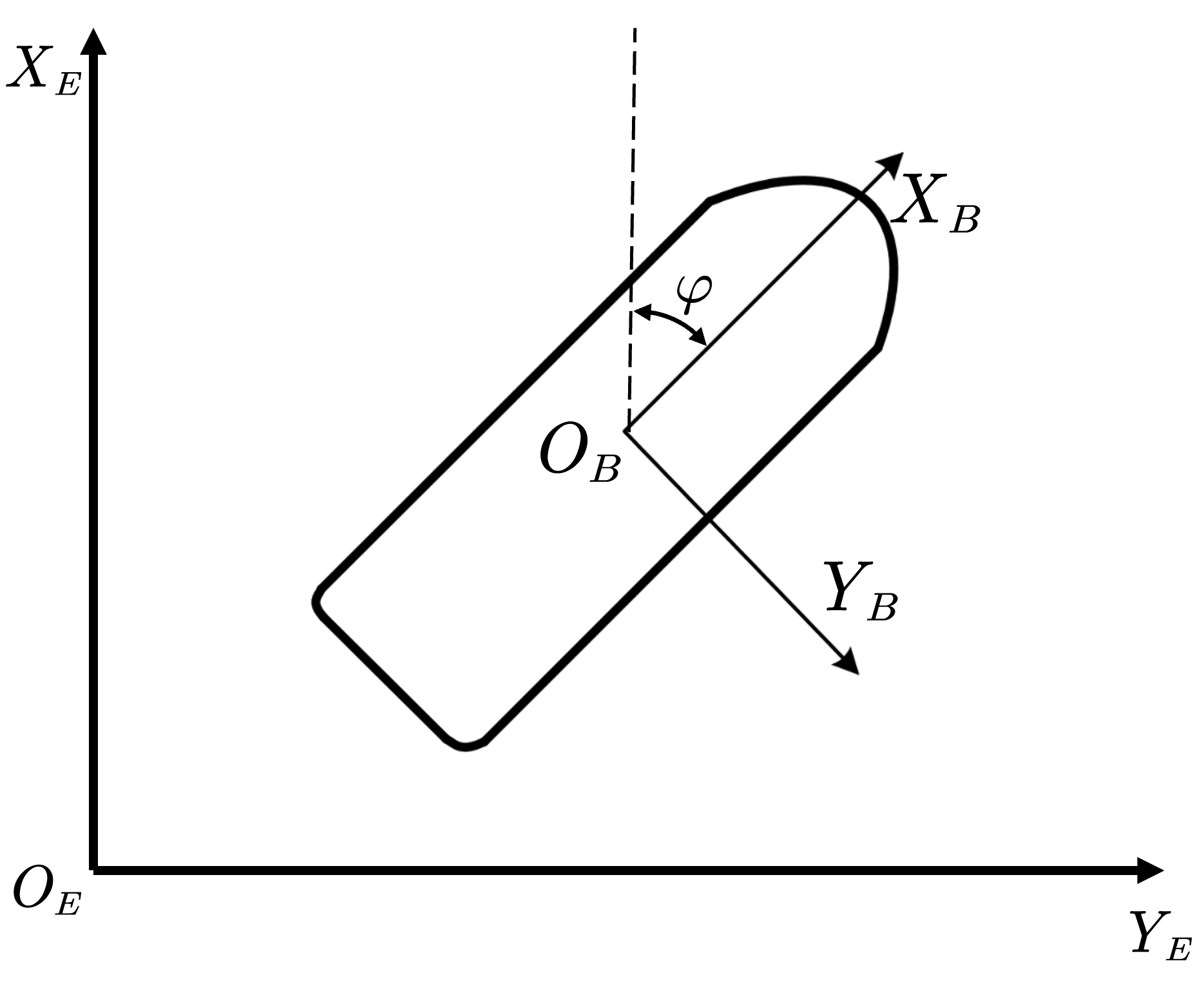
Figure 1: Schematic diagram of USVs planar motion (note: $X_{E}O_{E}Y_{E}$ are the earth-fixed reference frame, while $X_{B}O_{B}Y_{B}$ denote the body-fixed reference frame).

3.2 CLF-CBF-QP controller

From the section 2.3 and 2.4, we can construct the CLF-CBF-QP controller, which can be expressed as follows,

$$\min\frac{1}{2}u^{T}Hu+p\delta^{2}+\left\|x-x_{ref}\right\|_{Q}^{2}$$ (17a)

$$s.t.\,\, \mathcal{L}_{f}V\left(x\right)+\mathcal{L}_{g}V\left(x\right)u+\lambda V\left(x\right)\leqslant\delta$$ (17b)

$$\mathcal{L}_{f}B\left(x\right)+\mathcal{L}_{g}B\left(x\right)u+\gamma B\left(x\right)\geqslant 0$$ (17c)

$$u\in U$$ (17d)

Here, $H$, $p$, and $Q$ denote the weight coefficients of the control $u$, the relaxation factor $\delta$, and the weight coefficient of the error value between the actual trajectory $x$ and the reference trajectory $x_{ref}$, respectively. $u$ represents the control values, denoted as $\tau(\tau_{u},\tau_{v},\tau_{r})$ in this paper. $\delta$ is the slack variable of CLF that guarantees the feasibility of the problem. $\lambda$ and $\gamma$ represent the decay rate of the upper bound function $V(\cdot)$ in CLF and the decay rate of the lower bound function $B(\cdot)$ in CBF, respectively.

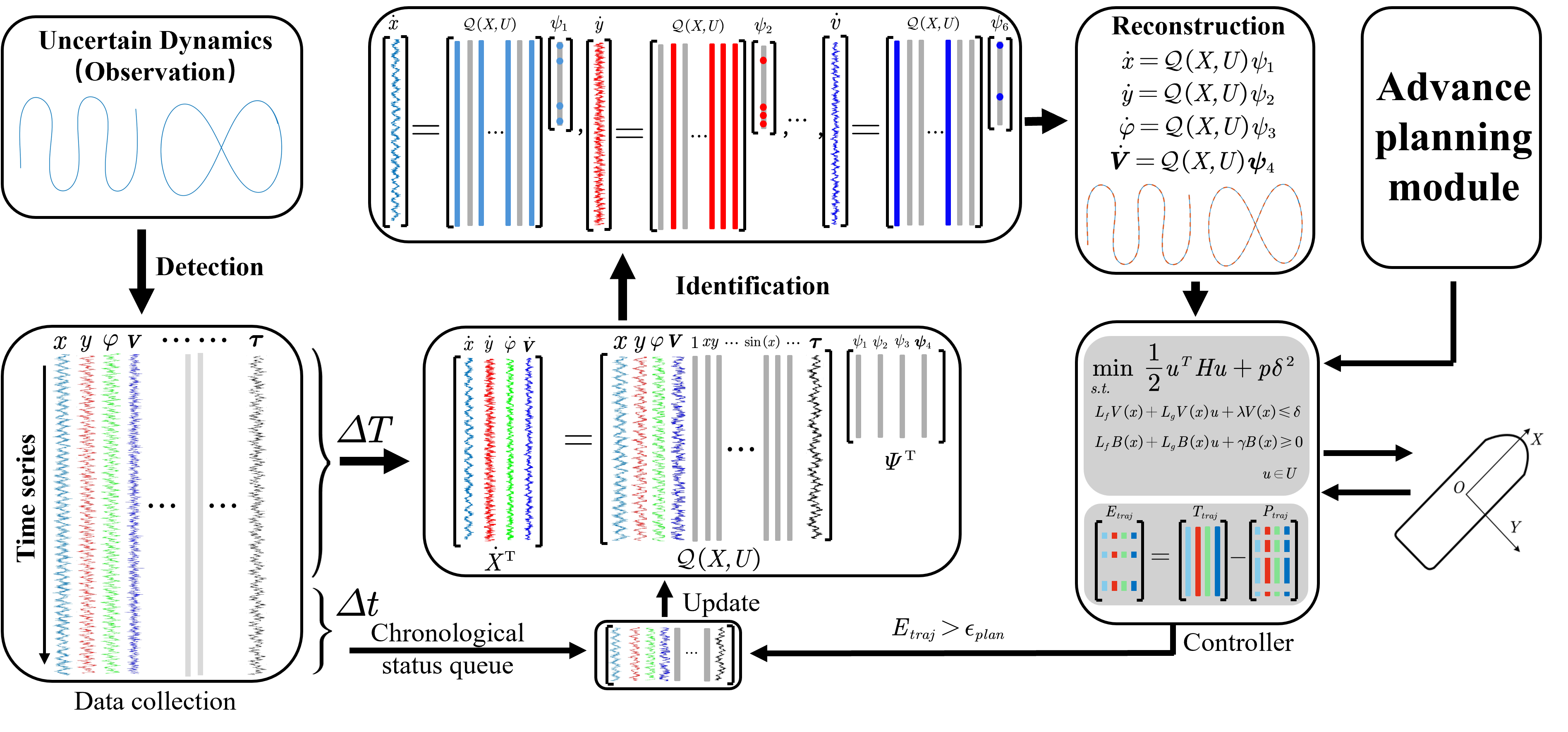
Figure 2: An example shows th

3.3 Framework of the system

The comprehensive architecture of the SINDy-online update with control framework is vividly illustrated in Fig.2. In this diagram, for the unknown dynamic system, the state position of the fuselage itself is obtained through the GPS and inertial measurement unit (IMU) onboard the USVs, and the torque of the control quantity is obtained through the sensor of the motor itself. After a period of time series data is collected, the original trajectory data of the dynamic system is obtained, as shown in the lower left corner of Fig.2.

Firstly, the identification module will perform sparse dynamic regression identification on the previously collected data within time T and obtain the derivative $\dot{X}$ of the state observation with respect to time by numerical methods. By collecting the time series of state and control quantities in time T for linear and nonlinear combinations, such as [$x$ $y$ $\varphi$ $xy$ $\cdots$ $sinx$ $\cdots$], to construct the candidate invariant subspace library $\mathcal{Q}$. Through iterative least squares, LASSO, and other methods, the best and smallest subspace of $\mathcal{Q}$ and the corresponding coefficient vector values are found for each observed state quantity, as shown in Fig.2, the middle and the upper part. Then, we can reconstruct the original nonlinear dynamic system approximately in higher-dimensional linear space, as illustrated in Fig.2 right and upper part. Thus, we can perform tracking control according to the previously planned path, utilizing trajectory information along the obtained high-dimensional linear affine dynamics model by constructing the CLF-CBF-QP controller in Section 3.2.

For time-invariant systems, this regression method can be employed to approximate the high-dimensional linear dynamics of the system. However, for nonlinear time-varying systems such as USVs, the parameters of the dynamic system itself are very complex, and the 3-degree-of-freedom (3-DOF) modeling and 6-DOF modeling are highly simplified physical models. If the interference of the external environment is considered, especially the influence of time-varying wind and waves, time-varying surges, tides, and other currents, it is challenging to reconstruct the dynamic characteristics of the system well using a fixed dynamic equation. Therefore, in this paper, we introduce a method to update the parameters of the system dynamics model in real-time, as shown in the lower right corner and lower part of Fig. 2.

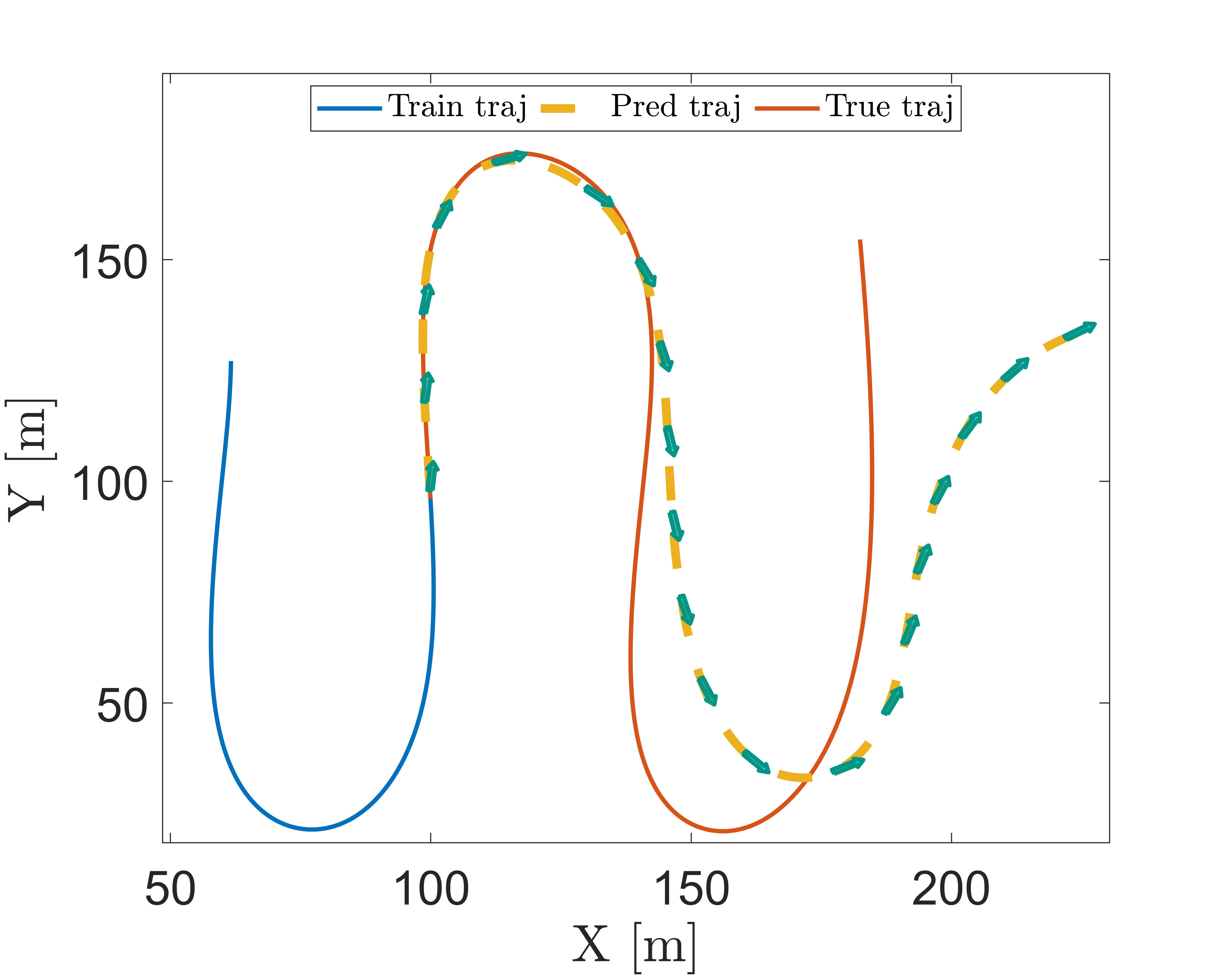
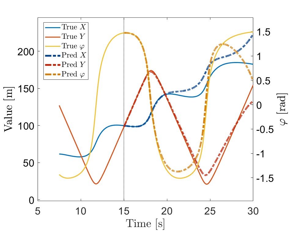
Figure 3: The blue trajectory part represents the training data for sparse regression, the red trajectory is obtained by controlling the USVs dynamics model, the yellow trajectory represents the predicted trajectory information obtained using the high-dimensional linear approximate affine dynamics model under the influence of the same control quantity, and the green arrow represents the heading angle of the USVs in (a). The state values during this situation, where the first 15 seconds represent the training set and the subsequent 15-30 seconds represent the predicted trajectory, are illustrated in (b), with $X$ and $Y$ using the left vertical axis, and $\varphi$ using the right axis.

If the entire system process is modeled, the parameters required for sparse dynamic regression would be extremely extensive, leading to a significant time and computational cost for data collection and regression. However, if only data information within a small time domain is used for sparse dynamic regression and identification, the data acquisition and calculation time can be significantly reduced, potentially meeting the computational requirements of online real-time regression. Nevertheless, training with data in a small time domain might result in inaccurate model parameters obtained by regression, as depicted in Fig.3. When only the data from the blue line part in the figure is used for sparse training, the obtained high-dimensional linear approximate affine dynamic model may initially match the original dynamic model 17 well. Still, as time progresses, the accumulated error increases, eventually causing the trajectory to deviate significantly (as shown in Fig.3, after 130m on the abscissa, and after 18s in Fig. 3).

Furthermore, even with a small amount of data, the real-time calculation method can significantly impact the load on the computing unit. In some extreme working conditions, it may affect the operational requirements of other equipment. Therefore, in this paper, we propose the error value trigger mode, which collects data online and triggers the update of system parameters based on the error value. This approach helps reduce the real-time computational demand. Specifically, the USVs’ pose and other observational values collected by sensors in real-time are used to calculate the error value $E_{traj}$ and the error threshold $\epsilon_{plan}$ between the current trajectory and the reference trajectory to be tracked. If $E_{traj}>\epsilon_{plan}$, the state variables collected in the previous time domain of delta-t from the current time are identified through sparse regression. The high-dimensional linear approximate affine dynamic model is then updated with the parameters obtained through regression, allowing the model to better match the environmental conditions.

4 Simulation

In this section, we designed two different scenarios: the long ’$S$’ trajectory and ’$8$’ trajectory for tracking using the SINDy-online update with CLF-CBF-Control system in the USVs model. We compare our method with other traditional control methods.

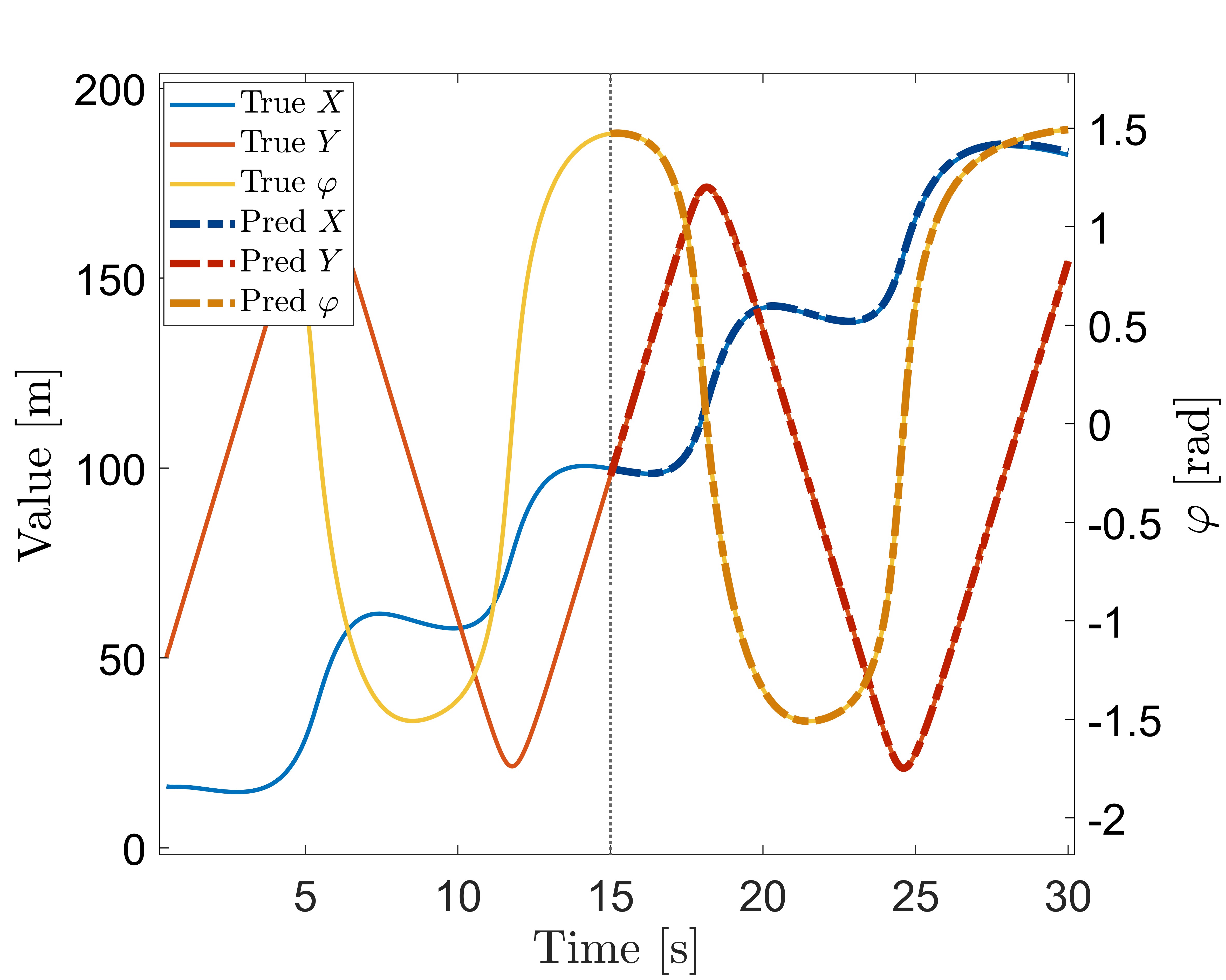
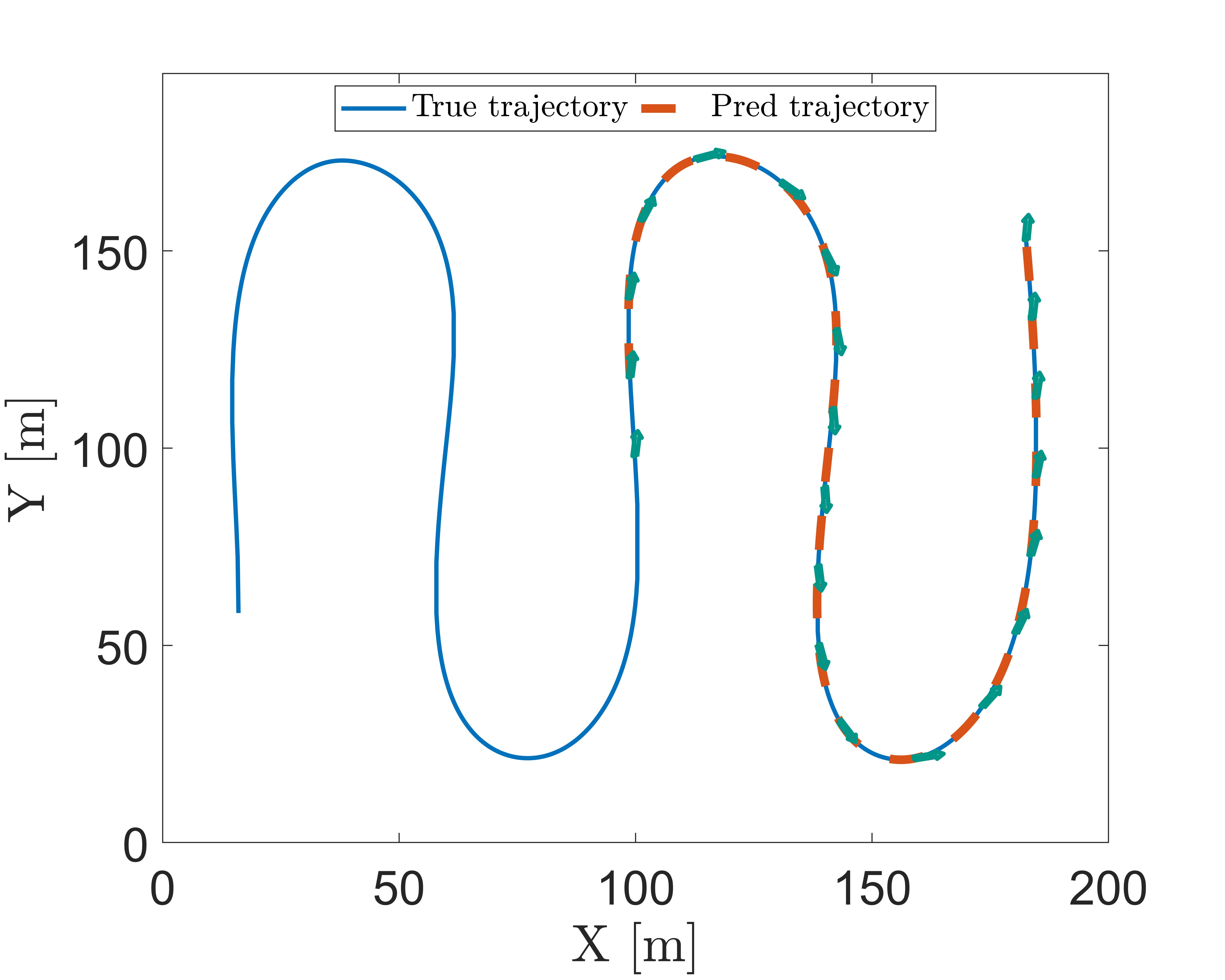
Figure 4: The left part of the dotted line represents the training data used for sparse dynamics regression. The solid line on the right of the dotted line is the predicted trajectory obtained by numerically integrating the high-dimensional linear approximate affine dynamics model derived from the original nonlinear dynamics regression after the application of the same control quantity. In 4, $X$ and $Y$ are on the left coordinate axis, and $\varphi$ is on the right coordinate axis. In 4, the trajectory is represented under the earth-fixed reference frame, where the green arrow denotes the orientation of the USVs.

In order to balance the speed of sparse regression and the accuracy of the constructed model, we determined through simulation experiments that the length of a short period of the training time domain is about 15s. This duration can lead to better trajectory prediction in a longer period of the time domain in the future. In other words, the high-dimensional approximate affine model is basically similar to the original nonlinear model. The simulation results are shown in Fig. 4.

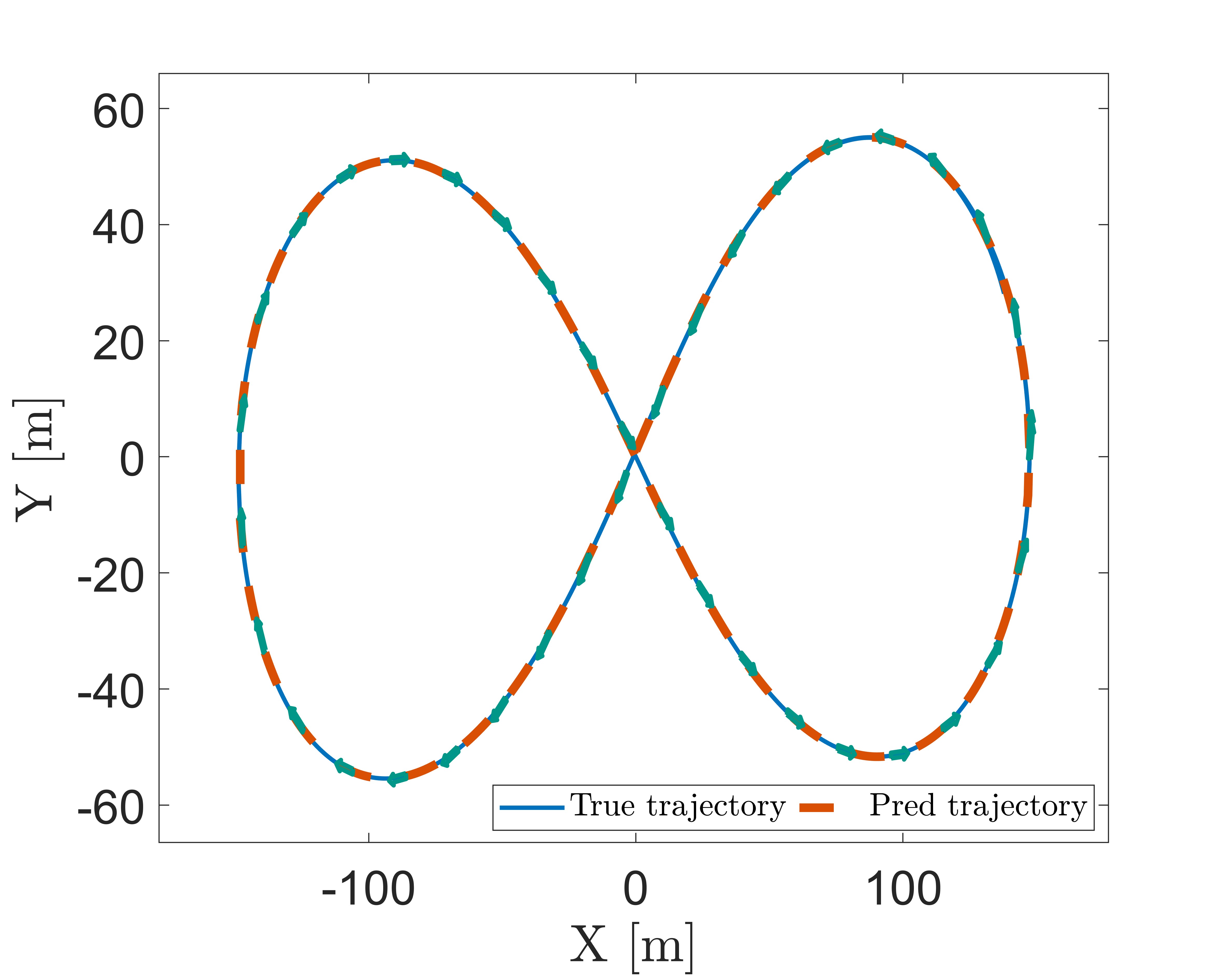
Figure 5: The original training trajectory information is compared with the predicted trajectory reconstructed by the high-dimensional linear approximate affine dynamics model obtained after sparse process regression.

In addition, we reconstruct the entire trajectory on the trained data, the long ’$S$’ and ’$8$’ are shown in Fig. 5.

So far, we have constructed a high-dimensional approximate linear affine model through the sparse dynamic regression model and successfully reconstructed the original trajectory. By introducing the reference trajectory, the error between the predicted trajectory of the current model and the reference trajectory that needs to be tracked is minimized under the action of the controller, as shown in Eq. 17a.

To further verify the characteristics of our proposed online sparse dynamics model regression with CLF-CBF-QP controller framework, we construct a tracking controller for the reference path through Eq.17 and compare the tracking effect with the nonlinear dynamics sliding mode control and the nonlinear dynamics CLF-CBF-QP controller under the condition of a uniform reference speed of 2 m/s. The comparative effect of tracking the ’$8$’ trajectory is shown in Fig.6, and the effect of tracking the variable telescopic ’$S$’ trajectory is shown in Fig. 7.

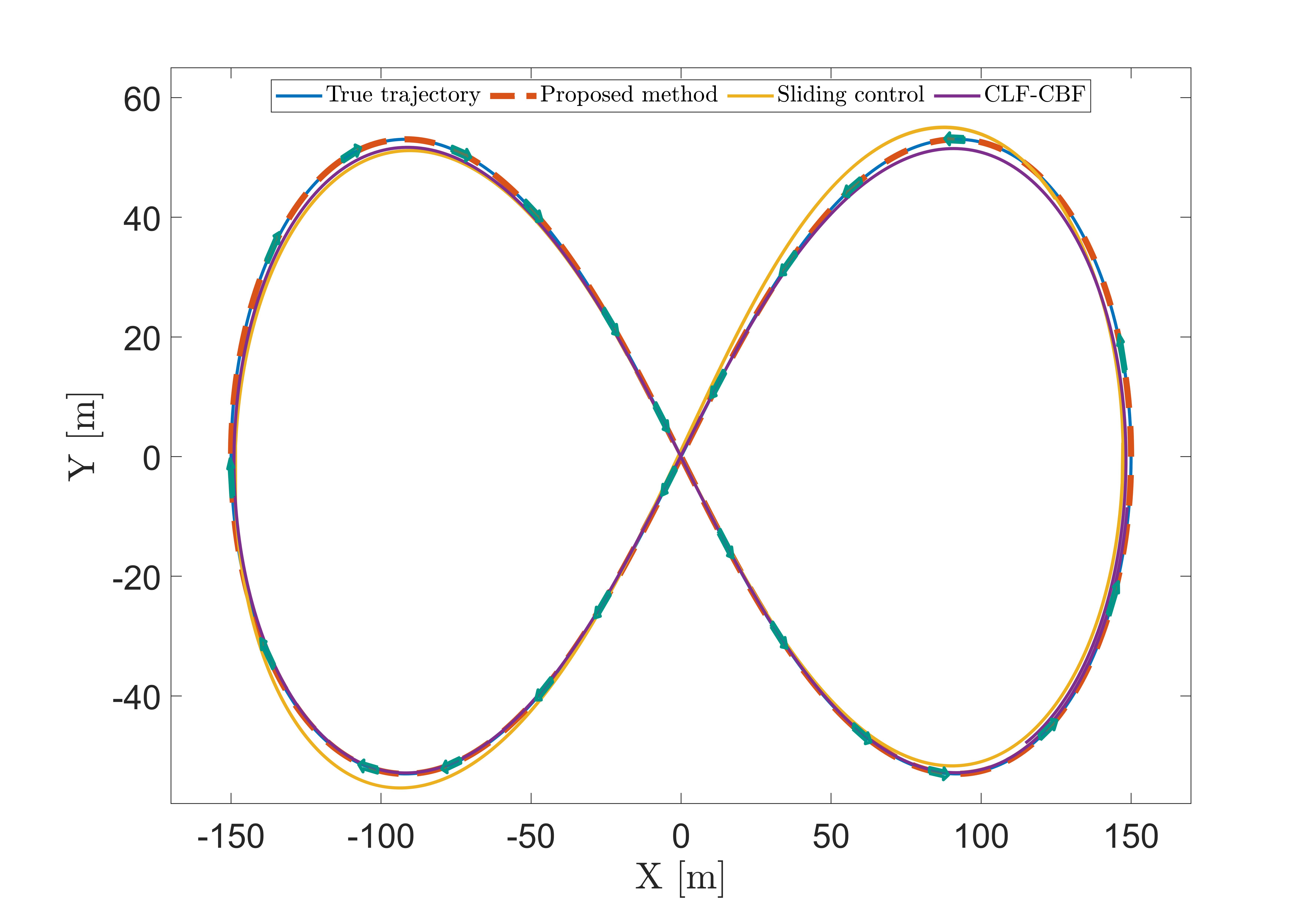
Figure 6: The comparative demonstration of the tracking effect of the ’$8$’ trajectory by different tracking control strategies in the earth-fixed coordinate system is presented. The blue line represents the reference path planned by the pre-trajectory planner, the red dotted line represents the method of updating the control framework of the online dynamics model proposed by us, and the yellow line is the tracking curve of the nonlinear dynamics model with sliding mode control. The purple line represents the tracking curve obtained by the nonlinear dynamics model with the CLF-CBF-QP controller.

Figure 7: The comparative demonstration of the tracking effect of the scalable ’$S$’ trajectory by different tracking control strategies in the earth-fixed coordinate system is shown. The blue line represents the reference path planned by the pre-trajectory planner, the red dotted line represents the method of updating the control framework of the online dynamics model proposed by us, and the yellow line is the tracking curve of the nonlinear dynamics model with sliding mode control. The purple line represents the tracking curve obtained by the nonlinear dynamics model with the CLF-CBF-QP controller.

From the comparison of different tracking controllers in Fig. 6 and 7, it is evident that our proposed methods of online sparse dynamics model update control achieve excellent tracking results.

5 Discussion and Conclusion

In this paper, we established a candidate sparse dynamic regression library using the collected USVs state trajectory information. We constructed the linear expansion of the original low-dimensional nonlinear dynamic model in high-dimensional space (high-dimensional linear approximate affine dynamic model) through the iterative least squares method and updated the linear approximate dynamic model in real time. Finally, the planned trajectory was tracked by the constructed CLF-CBF-QP controller. In the simulation experiment, compared with the tracking effect of the sliding mode controller with the nonlinear dynamic model and the nonlinear dynamic model in the CLF-CBF-QP controller, it can be concluded that our proposed online dynamic model update control method has significant tracking advantages.

However, due to experimental constraints, we did not conduct the tracking test in the physical model, and we also did not perform actual tests in time-varying environments (such as changing wind field influences and time-varying surge interference) and other scenarios with significant theoretical improvement. These aspects will be the focus of our further research and in-depth exploration in the future.

References

- Ames (2014) Ames, A.D., 2014. Human-inspired control of bipedal walking robots. IEEE Transactions on Automatic Control 59, 1115–1130.
- Annamalai et al. (2014) Annamalai, A.S., Sutton, R., Yang, C., Culverhouse, P., Sharma, S., 2014. Innovative adaptive autopilot design for uninhabited surface vehicles .
- Baek and Woo (2022) Baek, S., Woo, J., 2022. Model reference adaptive control-based autonomous berthing of an unmanned surface vehicle under environmental disturbance. Machines 10, 244.
- Berkooz et al. (1993) Berkooz, G., Holmes, P., Lumley, J.L., 1993. The proper orthogonal decomposition in the analysis of turbulent flows. Annual review of fluid mechanics 25, 539–575.
- Bongard and Lipson (2007) Bongard, J., Lipson, H., 2007. Automated reverse engineering of nonlinear dynamical systems. Proceedings of the National Academy of Sciences 104, 9943–9948.
- Brunton et al. (2017) Brunton, S.L., Brunton, B.W., Proctor, J.L., Kaiser, E., Kutz, J.N., 2017. Chaos as an intermittently forced linear system. Nature communications 8, 19.
- Brunton and Kutz (2022) Brunton, S.L., Kutz, J.N., 2022. Data-driven science and engineering: Machine learning, dynamical systems, and control. Cambridge University Press.
- Brunton et al. (2016) Brunton, S.L., Proctor, J.L., Kutz, J.N., 2016. Discovering governing equations from data by sparse identification of nonlinear dynamical systems. Proceedings of the national academy of sciences 113, 3932–3937.
- Cao et al. (2017) Cao, G., Lai, E.M.K., Alam, F., 2017. Gaussian process model predictive control of an unmanned quadrotor. Journal of Intelligent & Robotic Systems 88, 147–162.
- Chai and Sanfelice (2018) Chai, J., Sanfelice, R.G., 2018. Forward invariance of sets for hybrid dynamical systems (part i). IEEE Transactions on Automatic Control 64, 2426–2441.
- Chartrand (2011) Chartrand, R., 2011. Numerical differentiation of noisy, nonsmooth data. International Scholarly Research Notices 2011.
- Chen et al. (2014) Chen, T., Andersen, M.S., Ljung, L., Chiuso, A., Pillonetto, G., 2014. System identification via sparse multiple kernel-based regularization using sequential convex optimization techniques. IEEE Transactions on Automatic Control 59, 2933–2945.
- Dong et al. (2015) Dong, Z., Wan, L., Li, Y., Liu, T., Zhang, G., 2015. Trajectory tracking control of underactuated usv based on modified backstepping approach. International Journal of Naval Architecture and Ocean Engineering 7, 817–832.
- Du et al. (2022) Du, B., Lin, B., Zhang, C., Dong, B., Zhang, W., 2022. Safe deep reinforcement learning-based adaptive control for usv interception mission. Ocean Engineering 246, 110477.
- FosseN (2021) FosseN, T.I., 2021. Mathematical models of ships and underwater vehicles, in: Encyclopedia of systems and control. Springer, pp. 1–1.
- Gonzalez-Garcia and Castañeda (2021) Gonzalez-Garcia, A., Castañeda, H., 2021. Guidance and control based on adaptive sliding mode strategy for a usv subject to uncertainties. IEEE Journal of Oceanic Engineering 46, 1144–1154.
- Guerreiro et al. (2014) Guerreiro, B.J., Silvestre, C., Cunha, R., Pascoal, A., 2014. Trajectory tracking nonlinear model predictive control for autonomous surface craft. IEEE Transactions on Control Systems Technology 22, 2160–2175.
- Kaiser et al. (2018) Kaiser, E., Kutz, J.N., Brunton, S.L., 2018. Sparse identification of nonlinear dynamics for model predictive control in the low-data limit. Proceedings of the Royal Society A 474, 20180335.
- Koopman (1931) Koopman, B.O., 1931. Hamiltonian systems and transformation in hilbert space. Proceedings of the National Academy of Sciences 17, 315–318.
- Lee et al. (2019) Lee, K., Jeon, S., Kim, H., Kum, D., 2019. Optimal path tracking control of autonomous vehicle: Adaptive full-state linear quadratic gaussian (lqg) control. IEEE Access 7, 109120–109133.
- Li et al. (2008) Li, J.H., Lee, P.M., Jun, B.H., Lim, Y.K., 2008. Point-to-point navigation of underactuated ships. Automatica 44, 3201–3205.
- Liu et al. (2016) Liu, Z., Zhang, Y., Yu, X., Yuan, C., 2016. Unmanned surface vehicles: An overview of developments and challenges. Annual Reviews in Control 41, 71–93.
- Makaroff et al. (1995) Makaroff, D.J., Hutchinson, N.C., Neufeld, G.W., 1995. Department of computer science university of british columbia vancouver, bc v6t 1z4, canada .
- Mišković et al. (2011) Mišković, N., Vukić, Z., Bibuli, M., Bruzzone, G., Caccia, M., 2011. Fast in-field identification of unmanned marine vehicles. Journal of Field Robotics 28, 101–120.
- Oh and Sun (2010) Oh, S.R., Sun, J., 2010. Path following of underactuated marine surface vessels using line-of-sight based model predictive control. Ocean Engineering 37, 289–295.
- Rajesh and Bhattacharyya (2008) Rajesh, G., Bhattacharyya, S.K., 2008. System identification for nonlinear maneuvering of large tankers using artificial neural network. Applied Ocean Research 30, 256–263.
- Rudin et al. (1992) Rudin, L.I., Osher, S., Fatemi, E., 1992. Nonlinear total variation based noise removal algorithms. Physica D: nonlinear phenomena 60, 259–268.
- Schmid (2010) Schmid, P.J., 2010. Dynamic mode decomposition of numerical and experimental data. Journal of fluid mechanics 656, 5–28.
- Selvam et al. (2005) Selvam, R.P., Bhattacharyya, S., Haddara, M., 2005. A frequency domain system identification method for linear ship maneuvering. International shipbuilding progress 52, 5–27.
- Sutton et al. (2011) Sutton, R., Sharma, S., Xao, T., 2011. Adaptive navigation systems for an unmanned surface vehicle. Journal of Marine Engineering & Technology 10, 3–20.
- Tibshirani (1996) Tibshirani, R., 1996. Regression shrinkage and selection via the lasso. Journal of the Royal Statistical Society Series B: Statistical Methodology 58, 267–288.
- Wang et al. (2022) Wang, X., Liu, J., Peng, H., Qie, X., Zhao, X., Lu, C., 2022. A simultaneous planning and control method integrating apf and mpc to solve autonomous navigation for usvs in unknown environments. Journal of Intelligent & Robotic Systems 105, 36.
- Williams et al. (2015) Williams, M.O., Kevrekidis, I.G., Rowley, C.W., 2015. A data–driven approximation of the koopman operator: Extending dynamic mode decomposition. Journal of Nonlinear Science 25, 1307–1346.
- Wold et al. (1987) Wold, S., Esbensen, K., Geladi, P., 1987. Principal component analysis. Chemometrics and intelligent laboratory systems 2, 37–52.
- Xiao et al. (2022) Xiao, Y., Zhang, X., Xu, X., Liu, X., Liu, J., 2022. Deep neural networks with koopman operators for modeling and control of autonomous vehicles. IEEE Transactions on Intelligent Vehicles 8, 135–146.
- Xu et al. (2014) Xu, W., Bai, E.W., Cho, M., 2014. System identification in the presence of outliers and random noises: A compressed sensing approach. Automatica 50, 2905–2911.
- Yazdanpanah et al. (2013) Yazdanpanah, R., Mahjoob, M., Abbasi, E., 2013. Fuzzy lqr controller for heading control of an unmanned surface vessel, in: International Conference in Electrical and Electronics Engineering, pp. 73–78.
- Yeung et al. (2019) Yeung, E., Kundu, S., Hodas, N., 2019. Learning deep neural network representations for koopman operators of nonlinear dynamical systems, in: 2019 American Control Conference (ACC), IEEE. pp. 4832–4839.
- Zhang et al. (2011) Zhang, L.J., Jia, H.M., Qi, X., 2011. Nnffc-adaptive output feedback trajectory tracking control for a surface ship at high speed. Ocean Engineering 38, 1430–1438.
- Zhang et al. (2020) Zhang, S., Zhang, D., Qiao, J., Wang, X., Zhang, Z., 2020. Preventive control for power system transient security based on xgboost and dcopf with consideration of model interpretability. CSEE Journal of Power and Energy Systems 7, 279–294.