Velocities of mesenchymal cells maybe ill-defined
Introduction
Cell migration is a central mechanism in biological processes including tissue healing [1, 2], the immune defense [3], embryo development [4], and tumor evolution [5, 6, 7, 8, 9].
During migration, cells polarize as a result of the creation of gradients of protein concentration along their rear-front axis [10, 11, 12, 13]. These gradients are driven by active molecular transport facilitated by micro-tubule and actin fiber organization[14]. At the leading edge of the cell, actin monomers form a cytoskeletal network that extends against the cell membrane, creating a lamellipodium, which propels the entire cell forward through adhesion to the substrate followed by cytoskeletal contraction [15]. With the assistance of active transport of network components, the cell achieves stable and uniform movement [16, 17].
Although the dynamics of cell migration is typically uniform along the polarization direction of the cell during short periods, the polarization direction can change, and this creates a random walk for long periods. To model this migration pattern, Langevin-like equations are often used to predict the short-time ballistic motion and the long-time random walk.
On the other hand, a random motion regime has been experimentally observed for very short periods [18, 19, 20, 21, 22, 23, 24]. Instantaneous velocities, however, are impossible to be theoretically defined in this regime. The velocity in this case diverges and precludes the use of Langevin dynamics [25].
Additionally, cells do not migrate faster in chemical gradients. Rather, their orientations stabilize in the direction of the gradient, while their drift speeds stay approximately constant. This creates a displacement distribution that does not peak at zero [26, 9]. This contradicts the Langevin displacement distribution that peaks exactly at zero.
To address challenges related to diverging velocities, isotropic short-time random walks, and displacement distributions peaked at positive values, we propose a modified single cell migration model with three key components:
First, we introduce the concept of polarization, which guides the cell displacement for periods shorter than the polarization persistent time. Based on experimental observations of correlation between the displacement of the cell and its polarization [27, 28, 29], we define a polarization vector as a geometric object that can be obtained from a single shot image of the cell.
Second, we introduce an isotropic stochastic noise in the cellular position. This comes from the fact that passive transport lead to actin monomers polymerizing at the front part of the cell [15, 17]. This contributes, at least in part, to lamellipodia fluctuations and random walks at short periods.
Finally, we incorporate a drift bias into the model. This preference for forward motion is crucial for emulating the effects of active transport of cytoskeletal components over the cellular front, which results in uniform cellular motion [15, 17, 30]. The drift bias is also essential for chemotaxis, as it orients the polarization of the cell toward a chemical gradient, promoting forward motion. Without the drift bias, the cell would, on average, remain stationary even after aligning its polarization with the chemical gradient.
After establishing the foundational concepts of our topic, we will now provide a clear roadmap for the organization of our paper. We introduce our model for the cell dynamics in the next section. In section 3, we present the main results obtained from this model and compare them with other simulation strategies and experimental results. We conclude this paper in section 4 providing a discussion about the results and some propositions for further exploration.
The Model
A particle in our model is defined by a position vector and a polarization vector . In this last equation, is the polarization intensity and follows a Wiener process[31] such that:
| (1) |
where is normally distributed with expectation and variance given by:
| (2) |
The polarization intensity after a period is written in the form of a Langevin-like equation:
| (3) | |||
where corresponds to the cellular loss of polarity, is a Wiener process with zero expectation and variance given by . Also in the equation, is a constant bias responsible for inducing a forward biased movement of the cell with respect to the polarization axis. The product , corresponding to a unitary projection of the current polarization onto the polarization axis after a short interval, induces a loss of polarization intensity after the particle reorients.
The displacement of the particle is described by:
| (4) |
where is a proportionality constant between the cellular polarization and its displacement, is a Wiener process that models the phenomenon of fast polymerization and depolymerization of actin in the cytoskeleton. is the orientation of the polarization, while the orientation perpendicular to . Finally, implies that the two components of are uncorrelated. Note that the intensity of is proportional to the intensity of , through a proportionality constant . This is due to the fast polymerization-depolymerization phenomenon causing the turnover of both the positional random walk and the cellular polarization.
In summary, our model considers: 1) a point particle with a preferential direction of migration that changes according to the cell polarization reorientation given by the stochastic variable . 2) A displacement motion that is parallel to the preferential direction of migration and is proportional to the polarization intensity. This displacement captures the universal coupling between polarization and speed (UCPS) [28]. 3) An isotropic noise over the cellular displacement generated by whose purpose is to recreate the fast actin polymerization-depolymerization fluctuation.
Figure 1 shows a diagrammatic representation of our model.

Analytical Solution
The proposed model is solved considering the dynamics of the polarization magnitude for a single time step:
| (5) | |||||
This equation is then iterated to time with :
| (6) |
where the sub-index notation is used for simplicity. Every integral with respect to Wiener processes are Ito-integrable, which, can be represented as iterations.
The expected value of equation (6) is:
| (7) |
whose stationary average polarization is , corresponding to the polarization in the limit where . The variance of the polarization is obtained from its standard definition , giving:
| (8) |
Equations (7) and (8) evidence an asymptotic polarization distribution with constant variance and positive mean. Stated differently, the particle has a bias towards forward movement, since polarization and displacement are correlated. We call this phenomenon, the drift bias.
The particle’s position is the result of combining equations 4 and 6 for an arbitrary time-step and then summing it from to . This results in:
| (9) |
Equations (6) and (9) fully characterize the dynamics of our model through important functions such as the mean square displacement (MSD), the polarization autocorrelation function (PACF), the mean velocity auto-correlation function (mVACF) and the average velocity distribution function (VPDF). All of which will be explained next.
The polarization autocorrelation function, defined as , where the expectation is calculated over different noise realizations for every period :
| (10) | |||||
In short, the polarization of the particle has a memory and it decays as the sum of two exponential functions.
Twice differentiating Eq. (10) with respect to yields the mean square displacement (MSD), a measure that distinguishes ballistic from random walk regimes. Its analytical solution is written as:
| (11) | |||||
where are persistence coefficients, are diffusion coefficients, and represents the period where short-time random walk occurs. We call it the excess diffusion coefficient. Each coefficient is written in terms of the parameters of the model as:
| (12) | |||||
| (13) | |||||
| (14) | |||||
| (15) | |||||
| (16) |
The relation between the coefficients of diffusion, persistence, excess diffusion and the parameters of our model can be defined in many ways. However, relations 12-16 were written with the purpose of maintaining consistency with previous models [25]. Also, they facilitate the interpretation of each of the five coefficients, which can be determined experimentally. The experimental procedures for characterization in terms of the parameters of our model are explained at the end of this chapter.
We rewrite the MSD in its natural units, with . This gives:
| (17) | |||||
Expression (17) contains three parameters in the natural unit system: the persistence ratio , the diffusion ratio , and the excess diffusion coefficient .
The analytical MSD solution not only agrees with the numerical results of our model but also with CompuCell3D migration modelling results[32]. Where CompuCell3D is a Potts Modelling software [33] capable of reproducing the dynamics of certain systems through Monte Carlo energy minimization algorithms, a completely different approach from ours, but that has produced similar results. The model also supports the existence of the three observed migration regimes. They are characterized, in natural units, as random walk for , predominant ballistic motion for , and another random walk for . The persistence time changes according to . If , then is more significant than . However, if , then becomes the more important term, extending the time of persistence. These patterns have also been observed in various experiments conducted by different laboratories [18, 19, 20, 21, 22, 23, 24].
Using a normalized root mean square error (nRMSE) to quantify the quality of the fits, written as
| (18) |
where represents the experimental data-set, represents each of component of the experimental data-set and , the predicted values using our model and N is the size of the experimental data-set. With this, we are able to quantify the quality of the fits in percent terms with respect to the range of experimental values.
We obtained the following:
| Substrate Type | MSD | mVACF |
|---|---|---|
| Fibronectin | 0.68819 % | 0.08076 % |
| Collagen | 5.35556 % | 0.008507 % |
| Plastic | 0.05295 % | 0.18487 % |
and for the unbiased fits:
| Substrate Type | MSD | mVACF |
|---|---|---|
| Fibronectin | 0.78252 % | 0.19311 % |
| Collagen | 5.46699 % | 0.00807 % |
| Plastic | 0.20151 % | 0.18794 % |
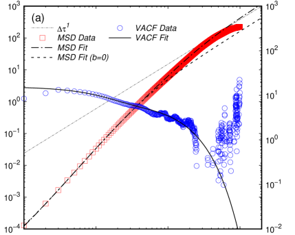
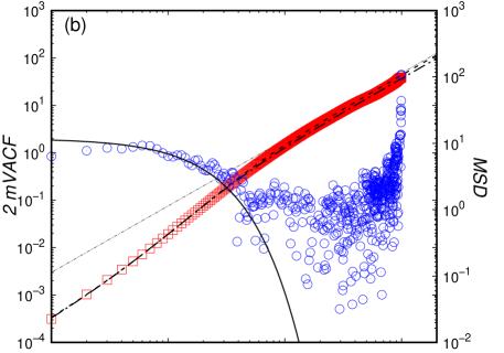
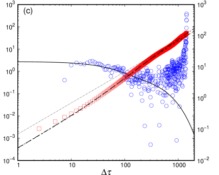
Figure 2 illustrates the steps for fitting experimental data for cell migration using the Levenberg-Marquardt algorithm [34, 35] in Gnuplot 5.4. The fitting process involves the following steps: (i) Estimating the parameter by analyzing the mVACF value at the beginning of its second regime. (ii) Exponential fitting the decay ratio and the initially estimated parameter for the second mVACF regime. (iii) Fitting the complete bi-exponential function (21) to determine , , , and . (iv) Fitting the excess-diffusion coefficient by fitting the MSD function (11).
Our model fits the calculated MSD and mVACF with experimental data better than our previous model based on an Ornstein-Uhlenbeck process [25] see tables (1,2) for the error comparison, see that for the fibronectin substrate we verify a reduction of more than half of the nRMSE. Moreover, the plots shown in Fig. 2 indicate that the experimental mVACF exhibit two different decay rates. Our model successfully captures this behavior. This is because the timings corresponding to a change in the polarization direction and the cell movement via acto-myosin mechanisms differ significantly, but equally affect the mVACF. Whereas the change in polarization affects the mVACF via memory loss, the cell movement affects the mVACF through short-time fluctuations in the cellular position.
There are two points, however, that should be clarified, the first is that Fig. (2) plot (c) shows an experimental mVACF with a slight decay for , which indicates a sub-diffusion process and may be indicative of anomalous migration [18, 23] something that is not encompassed by our model but that could be incorporated if desired. The second point is that in Fig. (2) plot (b), there where two stable fits that we managed to obtain, one that is shown in Fig. (2) and another that would produce a slightly better quality fit for the mVACF but worse values for the MSD (nRMSE=0.18794%) note however that in terms of the percent values of the total data range, all fits present very low root mean square errors.
The characterization of cellular dynamics is nearly complete by first measuring cell trajectories and time-series for the polarization, and then evaluating the MSD and PACF. However, there are not currently standardized protocols for measuring polarization time-series[29]. Therefore, the following discussion explains how to extract the polarization information from the trajectories.
Instantaneous displacements cannot be experimentally measured, since each successive microscope photography takes a finite period. Thus, although the position and polarization should ideally define the cellular dynamics fully, this interval should be accounted for. This issue is addressed by defining an average velocity as the ratio of a particle’s displacement in Eq. 4 and the elapsed time between consecutive measurements:
| (19) |
Because follows a Wiener process, the average velocity will exhibit different regimes described as follows: For very small values of , the ratio is significantly bigger than , resulting in a predominantly random walk behavior and an average velocity . When is sufficiently large (), . Consequently, the approximate average velocity becomes , which converges to a finite value. Such observation leads to a reliable definition of average velocity when a particle exhibits short-time random walk. We define the latter as the ratio of displacement and time during the interval when migration is mostly ballistic. This interval corresponds to the steepest slope in the mean square displacement (MSD) function.
Additionally, it is worth noting that for an intermediate value of , the auto-correlation function of is isomorphic to the polarization auto-correlation function (PACF), but scaled by the proportionality constant . This leads us to the concept of the mean velocity auto-correlation function (mVACF), denoted as , which factors in the finite time interval for each displacement value .
The analytical solution is found by combining equations (9) and:
| (20) |
in natural units, where and . The solution is given by:
| (21) | |||||
where the fractions after the exponential terms, with an hyperbolic cosine, can be interpreted as a correction factor that goes to as and , where is the polarization vector in natural units. The mVACF is proportional to PACF when the time between each successive displacement is exactly zero. The correction factor allows comparison between experimental displacement auto-correlation measurements with polarization auto-correlation obtained with our model even without having a polarization time-series data available.
The MSD, PACF and mVACF measurements distinguish random walk from ballistic regimes. However, these values are unable to characterize the drift bias or directional anisotropies such as chemoattraction. To model this effect, we also calculated the probability distribution function (PDF) for cellular displacements. Our earlier model, as presented in [25], featured a parallel-to-polarization probability density function (PDF) that peaks at zero. However, this outcome contradicts both single-cell migration experiments and the findings in chemotaxis, where particles are required to align themselves with a chemical gradient and exhibit forward movement as their preference. Therefore, it is necessary to include a bias in the Langevin equation corresponding to the polarization.
An analytical PDF for the particle’s polarization magnitude is obtained as follows. Assuming an infinitesimal variation in the PDF , we expand in a Taylor series and consider only the terms of second order or less in . With this, we obtain the Fokker-Planck equation[31] in natural units:
| (22) | |||||
where is the polarization magnitude in natural units, and are, respectively, the persistence and diffusion ratios. The stationary solution () for the Fokker-Planck equation (22) is a Gaussian function centered at or . This means that the particle has the highest probability of displacement proportional to , similar what is observed experimentally.
The polarization PDF can be experimentally obtained by measuring the cellular displacements during intervals when the ballistic regimes are mostly pronounced. The numerical results are shown in Fig. (LABEL:fig:avg_v_pdf).
Figure LABEL:fig:avg_v_pdf demonstrates that adjusting the time interval in the calculation affects both the shape and magnitude of the average velocity distributions. The first figure depicts a distribution with a peak at zero and a large variance, indicating that velocity values diverge when corresponds to a random walk regime. The second, third, and fourth figures show distributions with hollow centers and smaller variances, suggesting average velocity values centered around . The average velocity is obtained from solving the stationary Fokker-Planck equation considering all possible orientations. The fifth and sixth figures show distributions where most points lie at the center due to a significantly larger time interval as compared to the ballistic regime. This results in average velocities close to zero.
The results above show that the time interval has a high impact in the quality of the collected average velocity data and that there is an optimal time interval for measuring average velocities. An ideal experimental procedure for precise velocity measurements is to film the trajectories of some cells, obtain the mean square displacement and, through the analysis of the exponents of the mean square displacement curve, find the ideal time interval when the trajectory is mostly ballistic. The average displacement distribution should converge to the solution of equation 22, a non-zero Gaussian distribution.
The single cell migration model has five parameters, each modeling a certain cellular behavior. To compare the model with experiments, five different experimental values are needed. They may be determined by measuring the MSD, mVACF and the average velocity PDF. Even though we added one more parameter to describe the system, namely the drift bias, it does not add complications to the experimental analysis. The steps needed to compare the model with experiments are:
1. Acquire complete trajectory data and compute the resulting MSD to distinguish between distinct migration regimes: fast-time random walk, followed by the ballistic intermediate-time regime, and ultimately, long-time random walk.
2. Analyze the MSD curve to identify the time interval associated with the most pronounced ballistic migration regime, which is indicated by the steepest slope in the MSD. This process enables the determination of the optimal measurement interval for defining average velocities.
3. Utilize the optimal time interval to calculate cellular displacements and generate a distribution of average velocities. Subsequently, evaluate the mean and variance of the distribution, which in the model are represented by and , respectively.
4. Compute the values of the mVACF and observe its rate of decay. If only one rate of exponential decay is observed, it becomes challenging to distinguish the noise component from the drift bias. In such case, the experimental analysis should follow the approach described in [25]. However, if two distinct regimes can be identified, as in Fig. (2), fit the mVACF solution to data to extract the two decay rates and the associated coefficients .
5. Fit the MSD function 11 to the experimental data together with the previously obtained parameters to determine the excess diffusion coefficient .
6. Determine the ratio between the persistence coefficients and the diffusion coefficients and calculate the MSD in natural units.
Such procedure fully characterizes experimental data and allows one to compare simulations of different cell strands and single cell dynamics. The only unexplained phenomenon in our model is a correlation decay in mVACF for small values. In [25], we explained that taking the average of a squared cell displacement that is consistent with a well defined converging part and a random walk part, would incur in loss of correlation. While this theory, due to finite precision measurements, should manifest experimentally, it is intriguing that the decrease in correlation is also observed in CompuCell3D cell simulations, which have sufficient precision. This similarity in correlation decay for suggests that, while part of the decay may be attributed to the finite precision of measurements, there must exist another contributing factor [18].
Discussions and Concluding Remarks
We have shown that a model that incorporates spatial anisotropy can accurately simulate cellular motion. Cells, however, have asymmetric cytoskeletal structures that facilitate their migration, which makes orientation anisotropy alone fail to replicate experimental results. Each cell also experience noise in all directions, which arises from the passive transport of actin filaments within its interior[15, 17]. Consequently, defining instantaneous velocities becomes challenging. To analyze cellular motion effectively, we propose a quantity that remains well-defined, regardless of the time interval used to measure cellular displacements.
Previous research [28] shows that the correlation between cellular displacements and cell polarization is well established. Cell polarization, characterized by a geometrical quantity given by a vector connecting the cellular center of mass to its nucleus, always remains well-defined. By considering this polarization for measuring displacement, we were able to introduce noise into the particle’s movement. This approach maintains a well-defined displacement while promoting a biased forward motion, which enables migration under a chemical field. Remarkably, this model reproduces the three migration regimes observed experimentally.
In cases where the polarization data is not available, one can still analyze cellular dynamics satisfactorily by determining the optimal time interval (corresponding to the highest slope in the MSD) that ensures a well-defined and converging average velocity. Subsequently, calculations of the mVACF and the average velocity PDF can provide more insights. These measurements quantify crucial aspects of cellular dynamics, such as the extent of position fluctuations, the typical average velocity of cell migration, the way polarization orientation changes, and the transition from a random walk to a ballistic behavior in a trajectory.
In conclusion, our model captures most of the characteristics of single cell dynamics. And although there are some different approaches such as active bio-fluid models (see for instance [36, 37]), these techniques would still not be sufficient to reproduce specific individual behaviors described by our model, even if the case of non interacting fluid particles. For instance, our model provides a mean velocity distribution where the peak assumes positive values. Moreover, the mean velocity autocorrelation function (mVACF) in our model shows a bi-exponential decay, implying processes that decrease at different rates. This behavior depends on timing of processes related to the polarization orientation change and the internal cytoskeletal rearrangement which exhibit different characteristic time-scales.
References
- [1] Basan, M., Elgeti, J., Hannezo, E., Rappel, W. J. & Levine, H. Alignment of cellular motility forces with tissue flow as a mechanism for efficient wound healing. Proceedings of the National Academy of Sciences of the United States of America 110, 2452–2459 (2013). URL www.pnas.org/cgi/doi/10.1073/pnas.1219937110.
- [2] Cui, B. et al. Collagen-tussah silk fibroin hybrid scaffolds loaded with bone mesenchymal stem cells promote skin wound repair in rats. Materials Science and Engineering C 109, 110611 (2020).
- [3] Qi, K., Li, N., Zhang, Z. & Melino, G. Tissue regeneration: The crosstalk between mesenchymal stem cells and immune response. Cellular Immunology 326, 86–93 (2018).
- [4] Alt, S., Ganguly, P. & Salbreux, G. Vertex models: from cell mechanics to tissue morphogenesis. Philosophical Transactions of the Royal Society B: Biological Sciences 372, 20150520 (2017). URL https://royalsocietypublishing.org/doi/10.1098/rstb.2015.0520.
- [5] Wolf, K. et al. Multi-step pericellular proteolysis controls the transition from individual to collective cancer cell invasion. Nature Cell Biology 9, 893–904 (2007). URL https://www.nature.com/articles/ncb1616.
- [6] Friedl, P. & Alexander, S. Cancer invasion and the microenvironment: Plasticity and reciprocity. Cell 147, 992–1009 (2011). URL http://www.cell.com/article/S0092867411013547/fulltexthttp://www.cell.com/article/S0092867411013547/abstracthttps://www.cell.com/cell/abstract/S0092-8674(11)01354-7.
- [7] Kabla, A. J. Collective cell migration: leadership, invasion and segregation. Journal of The Royal Society Interface 9, 3268–3278 (2012). URL https://royalsocietypublishing.org/doi/10.1098/rsif.2012.0448.
- [8] Szabó, A. & Merks, R. M. Cellular potts modeling of tumor growth, tumor invasion, and tumor evolution. Frontiers in Oncology 3 APR, 87 (2013). URL www.frontiersin.org.
- [9] Nousi, A., Søgaard, M. T., Audoin, M. & Jauffred, L. Single-cell tracking reveals super-spreading brain cancer cells with high persistence. Biochemistry and Biophysics Reports 28, 101120 (2021).
- [10] Stossel, T. P. How cells crawl. American Scientist 78, 408–423 (1990). URL http://www.jstor.org/stable/29774178.
- [11] Hall, A. & Nobes, C. D. Rho gtpases: Molecular switches that control the organization and dynamics of the actin cytoskeleton. Philosophical Transactions of the Royal Society B: Biological Sciences 355, 965–970 (2000). URL https://royalsocietypublishing.org/doi/abs/10.1098/rstb.2000.0632.
- [12] Marée, A. F., Jilkine, A., Dawes, A., Grieneisen, V. A. & Edelstein-Keshet, L. Polarization and movement of keratocytes: A multiscale modelling approach. Bulletin of Mathematical Biology 68, 1169–1211 (2006). URL http://theory.bio.uu.nl/stan/keratocyte.
- [13] Hennig, K. et al. Stick-slip dynamics of cell adhesion triggers spontaneous symmetry breaking and directional migration of mesenchymal cells on one-dimensional lines. Science Advances 6 (2020).
- [14] Bugyi, B. & Kellermayer, M. The discovery of actin: “to see what everyone else has seen, and to think what nobody has thought”*. Journal of Muscle Research and Cell Motility 41, 3–9 (2020). URL https://doi.org/10.1007/s10974-019-09515-z.
- [15] Mogilner, A. Mathematics of cell motility: Have we got its number? Journal of Mathematical Biology 58, 105–134 (2009). URL https://link.springer.com/article/10.1007/s00285-008-0182-2.
- [16] Shao, D., Levine, H. & Rappel, W. J. Coupling actin flow, adhesion, and morphology in a computational cell motility model. Proceedings of the National Academy of Sciences of the United States of America 109, 6851–6856 (2012). URL https://www.pnas.org/content/109/18/6851https://www.pnas.org/content/109/18/6851.abstract.
- [17] Mogilner, A., Barnhart, E. L. & Keren, K. Experiment, theory, and the keratocyte: An ode to a simple model for cell motility. Seminars in Cell and Developmental Biology 100, 143–151 (2020).
- [18] Selmeczi, D., Mosler, S., Hagedorn, P. H., Larsen, N. B. & Flyvbjerg, H. Cell motility as persistent random motion: Theories from experiments. Biophysical Journal 89, 912–931 (2005).
- [19] Dieterich, P., Klages, R., Preuss, R. & Schwab, A. Anomalous dynamics of cell migration. Proceedings of the National Academy of Sciences of the United States of America 105, 459–463 (2008). URL www.pnas.orgcgidoi10.1073pnas.0707603105.
- [20] Potdar, A. A., Lu, J., Jeon, J., Weaver, A. M. & Cummings, P. T. Bimodal analysis of mammary epithelial cell migration in two dimensions. Annals of Biomedical Engineering 37, 230–245 (2009). URL https://link.springer.com/article/10.1007/s10439-008-9592-y.
- [21] Gruver, J. S. et al. Bimodal analysis reveals a general scaling law governing nondirected and chemotactic cell motility. Biophysical Journal 99, 367–376 (2010).
- [22] Wu, P. H., Giri, A., Sun, S. X. & Wirtz, D. Three-dimensional cell migration does not follow a random walk. Proceedings of the National Academy of Sciences of the United States of America 111, 3949–3954 (2014). URL https://www.pnas.org/content/111/11/3949https://www.pnas.org/content/111/11/3949.abstract.
- [23] Metzner, C. et al. Superstatistical analysis and modelling of heterogeneous random walks. Nature Communications 6 (2015).
- [24] Thomas, G. L. et al. Parameterizing cell movement when the instantaneous cell migration velocity is ill-defined. Physica A: Statistical Mechanics and its Applications 550, 124493 (2020).
- [25] de Almeida, R. M., Giardini, G. S., Vainstein, M., Glazier, J. A. & Thomas, G. L. Exact solution for the anisotropic ornstein–uhlenbeck process. Physica A: Statistical Mechanics and its Applications 587, 126526 (2022).
- [26] Masuzzo, P. et al. An end-to-end software solution for the analysis of high-throughput single-cell migration data. Scientific Reports 7 (2017).
- [27] Directing cell migration with asymmetric micropatterns. Proceedings of the National Academy of Sciences of the United States of America 102, 975–978 (2005). URL https://www.pnas.org/doi/abs/10.1073/pnas.0408954102.
- [28] Callan-Jones, A. C. & Voituriez, R. Actin flows in cell migration: From locomotion and polarity to trajectories. Current Opinion in Cell Biology 38, 12–17 (2016). URL https://pubmed.ncbi.nlm.nih.gov/26827283/.
- [29] Thomas, G. L., Fortuna, I., Perrone, G. C., Graner, F. & de Almeida, R. M. Shape–velocity correlation defines polarization in migrating cell simulations. Physica A: Statistical Mechanics and its Applications 587, 126511 (2022).
- [30] Allen, G. M. et al. Cell mechanics at the rear act to steer the direction of cell migration. Cell Systems 11, 286–299.e4 (2020). URL http://www.cell.com/article/S2405471220302921/fulltexthttp://www.cell.com/article/S2405471220302921/abstracthttps://www.cell.com/cell-systems/abstract/S2405-4712(20)30292-1.
- [31] da Cunha, C. R. Introduction to Econophysics: contemporary approaches with Python simulations (CRC Press, Boca Raton, FL, 2021), 1 edn.
- [32] Fortuna, I. et al. Compucell3d simulations reproduce mesenchymal cell migration on flat substrates. Biophysical Journal 118, 2801–2815 (2020).
- [33] Graner, F. & Glazier, J. A. Simulation of biological cell sorting using a two-dimensional extended potts model. Physical Review Letters 69, 2013–2016 (1992). URL https://journals.aps.org/prl/abstract/10.1103/PhysRevLett.69.2013.
- [34] Levenberg, K. A method for the solution of certain non-linear problems in least squares. Quarterly of Applied Mathematics 2, 164–168 (1944).
- [35] Marquardt, D. W. An algorithm for least-squares estimation of nonlinear parameters. Journal of the Society for Industrial and Applied Mathematics 11, 431–441 (1963). URL http://www.jstor.org/stable/2098941.
- [36] Martin, D. et al. Statistical mechanics of active ornstein-uhlenbeck particles. Physical Review E 103, 032607 (2021). URL https://journals.aps.org/pre/abstract/10.1103/PhysRevE.103.032607.
- [37] Étienne Fodor, Jack, R. L. & Cates, M. E. Irreversibility and biased ensembles in active matter: Insights from stochastic thermodynamics. Annual Review of Condensed Matter Physics 13, 215–238 (2021). URL http://arxiv.org/abs/2104.06634http://dx.doi.org/10.1146/annurev-conmatphys-031720-032419.
- [38] Rens, E. G. & Merks, R. M. Cell contractility facilitates alignment of cells and tissues to static uniaxial stretch. Biophysical Journal 112, 755–766 (2017). URL http://dx.doi.org/10.1016/j.bpj.2016.12.012.
- [39] Albert, P. J. & Schwarz, U. S. Dynamics of cell ensembles on adhesive micropatterns: Bridging the gap between single cell spreading and collective cell migration. PLOS Computational Biology 12, e1004863 (2016). URL https://dx.plos.org/10.1371/journal.pcbi.1004863.
- [40] Honda, H. Description of cellular patterns by dirichlet domains: The two-dimensional case. Journal of Theoretical Biology 72, 523–543 (1978).
- [41] Li, B. & Sun, S. X. Coherent motions in confluent cell monolayer sheets. Biophysical Journal 107, 1532–1541 (2014). URL http://dx.doi.org/10.1016/j.bpj.2014.08.006.
- [42] Gardiner, B. S. et al. Discrete element framework for modelling extracellular matrix, deformable cells and subcellular components. PLOS Computational Biology 11, e1004544 (2015). URL https://dx.plos.org/10.1371/journal.pcbi.1004544.
- [43] Niculescu, I., Textor, J. & de Boer, R. J. Crawling and gliding: A computational model for shape-driven cell migration. PLOS Computational Biology 11, e1004280 (2015). URL https://dx.plos.org/10.1371/journal.pcbi.1004280.
- [44] Segerer, F. J., Thüroff, F., Alberola, A. P., Frey, E. & Rädler, J. O. Emergence and persistence of collective cell migration on small circular micropatterns. Physical Review Letters 114, 228102 (2015). URL https://journals.aps.org/prl/abstract/10.1103/PhysRevLett.114.228102.
- [45] van Oers, R. F., Rens, E. G., LaValley, D. J., Reinhart-King, C. A. & Merks, R. M. Mechanical cell-matrix feedback explains pairwise and collective endothelial cell behavior in vitro. PLoS Computational Biology 10, 1003774 (2014). URL www.ploscompbiol.org.
- [46] Löber, J., Ziebert, F. & Aranson, I. S. Collisions of deformable cells lead to collective migration. Scientific Reports 5, 1–7 (2015). URL www.nature.com/scientificreports.
- [47] Camley, B. A. & Rappel, W. J. Velocity alignment leads to high persistence in confined cells. Physical Review E - Statistical, Nonlinear, and Soft Matter Physics 89, 062705 (2014). URL https://journals.aps.org/pre/abstract/10.1103/PhysRevE.89.062705.
- [48] Camley, B. A. et al. Polarity mechanisms such as contact inhibition of locomotion regulate persistent rotational motion of mammalian cells on micropatterns. Proceedings of the National Academy of Sciences of the United States of America 111, 14770–14775 (2014). URL www.pnas.org/cgi/doi/10.1073/pnas.1414498111.
- [49] Ziebert, F., Swaminathan, S. & Aranson, I. S. Model for self-polarization and motility of keratocyte fragments. Journal of The Royal Society Interface 9, 1084–1092 (2012). URL https://royalsocietypublishing.org/doi/10.1098/rsif.2011.0433.
- [50] Shao, D., Rappel, W. J. & Levine, H. Computational model for cell morphodynamics. Physical Review Letters 105, 108104 (2010). URL https://journals.aps.org/prl/abstract/10.1103/PhysRevLett.105.108104.
- [51] Tarle, V. et al. Modeling collective cell migration in geometric confinement. Physical Biology 14, 035001 (2017). URL https://iopscience.iop.org/article/10.1088/1478-3975/aa6591https://iopscience.iop.org/article/10.1088/1478-3975/aa6591/meta.
- [52] Banerjee, S., Utuje, K. J. & Marchetti, M. C. Propagating stress waves during epithelial expansion. Physical Review Letters 114, 228101 (2015). URL https://journals.aps.org/prl/abstract/10.1103/PhysRevLett.114.228101.
- [53] Szabó, A. et al. Collective cell motion in endothelial monolayers. Physical Biology 7, 046007 (2010). URL https://iopscience.iop.org/article/10.1088/1478-3975/7/4/046007https://iopscience.iop.org/article/10.1088/1478-3975/7/4/046007/meta.
- [54] Sepúlveda, N. et al. Collective cell motion in an epithelial sheet can be quantitatively described by a stochastic interacting particle model. PLoS Computational Biology 9, 1002944 (2013). URL www.ploscompbiol.org.
- [55] Szabó, B. et al. Phase transition in the collective migration of tissue cells: Experiment and model. Physical Review E - Statistical, Nonlinear, and Soft Matter Physics 74, 061908 (2006). URL https://journals.aps.org/pre/abstract/10.1103/PhysRevE.74.061908.
- [56] Goychuk, A. et al. Morphology and motility of cells on soft substrates. arXiv (2018). URL http://arxiv.org/abs/1808.00314.
- [57] Dietrich, M. et al. Guiding 3d cell migration in deformed synthetic hydrogel microstructures. Soft Matter 14, 2816–2826 (2018). URL https://pubs.rsc.org/en/content/articlehtml/2018/sm/c8sm00018bhttps://pubs.rsc.org/en/content/articlelanding/2018/sm/c8sm00018b.
- [58] Albert, P. J. & Schwarz, U. S. Dynamics of cell shape and forces on micropatterned substrates predicted by a cellular potts model. Biophysical Journal 106, 2340–2352 (2014). URL http://dx.doi.org/10.1016/j.bpj.2014.04.036.
- [59] Camley, B. A., Zhao, Y., Li, B., Levine, H. & Rappel, W. J. Periodic migration in a physical model of cells on micropatterns. Physical Review Letters 111, 158102 (2013). URL https://journals.aps.org/prl/abstract/10.1103/PhysRevLett.111.158102.
- [60] Ziebert, F. & Aranson, I. S. Effects of adhesion dynamics and substrate compliance on the shape and motility of crawling cells. PLoS ONE 8, 64511 (2013). URL www.plosone.org.
- [61] Marée, A. F., Grieneisen, V. A. & Edelstein-Keshet, L. How cells integrate complex stimuli: The effect of feedback from phosphoinositides and cell shape on cell polarization and motility. PLoS Computational Biology 8, e1002402 (2012). URL http://royalsociety.org/grants/schemes/dorothy-hodgkin/.
- [62] Thüroff, F., Goychuk, A., Reiter, M. & Frey, E. Bridging the gap between single-cell migration and collective dynamics. eLife 8 (2019).
- [63] Turing, A. M. The chemical basis of morphogenesis (1952). URL http://www.jstor.org/about/terms.html.
- [64] Vicsek, T., Czirk, A., Ben-Jacob, E., Cohen, I. & Shochet, O. Novel type of phase transition in a system of self-driven particles. Physical Review Letters 75, 1226–1229 (1995). URL https://journals.aps.org/prl/abstract/10.1103/PhysRevLett.75.1226.
- [65] Ross, H. C. On a combination of substances which excites amŒboid movement in leucocytes, by which living can be differentiated from dead cells. The Lancet 173, 152–154 (1909).
- [66] W.H.C. Ciliary movement. American Journal of Ophthalmology 11, 825 (1928). URL http://www.ajo.com/article/S0002939428928706/fulltext.
- [67] Fürth, R. Die brownsche bewegung bei berücksichtigung einer persistenz der bewegungsrichtung. mit anwendungen auf die bewegung lebender infusorien. Zeitschrift für Physik 2, 244–256 (1920).
- [68] Peruani, F. & Morelli, L. G. Self-propelled particles with fluctuating speed and direction of motion in two dimensions. Physical Review Letters 99, 010602 (2007). URL https://journals.aps.org/prl/abstract/10.1103/PhysRevLett.99.010602.
- [69] Palsson, E. & Othmer, H. G. A model for individual and collective cell movement in dictyostelium discoideum. Proceedings of the National Academy of Sciences of the United States of America 97, 10448–10453 (2000). URL /pmc/articles/PMC27044/?report=abstracthttps://www.ncbi.nlm.nih.gov/pmc/articles/PMC27044/.
- [70] Camley, B. A. & Rappel, W. J. Physical models of collective cell motility: From cell to tissue. Journal of Physics D: Applied Physics 50, 113002 (2017). URL https://iopscience.iop.org/article/10.1088/1361-6463/aa56fehttps://iopscience.iop.org/article/10.1088/1361-6463/aa56fe/meta.
- [71] Lämmermann, T. & Sixt, M. Mechanical modes of ’amoeboid’ cell migration. Current Opinion in Cell Biology 21, 636–644 (2009).
- [72] Hall, A. Rho gtpases and the actin cytoskeleton. Science 279, 509–514 (1998). URL https://science.sciencemag.org/content/279/5350/509https://science.sciencemag.org/content/279/5350/509.abstract.
- [73] Kholodenko, B. N. Cell-signalling dynamics in time and space. Nature Reviews Molecular Cell Biology 7, 165–176 (2006). URL www.nature.com/reviews/molcellbio.
- [74] Merchant, B., Edelstein-Keshet, L. & Feng, J. J. A rho-gtpase based model explains spontaneous collective migration of neural crest cell clusters. Developmental Biology 444, S262–S273 (2018).
- [75] Gail, M. H. & Boone, C. W. The locomotion of mouse fibroblasts in tissue culture. Biophysical Journal 10, 980–993 (1970).
- [76] Genthon, A. The concept of velocity in the history of brownian motion – from physics to mathematics and vice versa. European Physical Journal H 45, 49–105 (2020). URL http://arxiv.org/abs/2006.05399http://dx.doi.org/10.1140/epjh/e2020-10009-8.
- [77] Maiuri, P. et al. Actin flows mediate a universal coupling between cell speed and cell persistence. Cell 161, 374–386 (2015). URL https://pubmed.ncbi.nlm.nih.gov/25799384/.
- [78] Giardini, G. S. Y. & Alegre, P. A proper velocity measure for mesenchymal cells migration (2022). URL https://lume.ufrgs.br/handle/10183/240303.
- [79] Lemons, D. S. & Gythiel, A. Paul langevin’s 1908 paper “on the theory of brownian motion” [“sur la théorie du mouvement brownien,” c. r. acad. sci. (paris) 146 , 530–533 (1908)]. American Journal of Physics 65, 1079–1081 (1997). URL http://aapt.scitation.org/doi/10.1119/1.18725.