Spatial-Temporal Extreme Modeling for Point-to-Area Random Effects (PARE)

Abstract

One measurement modality for rainfall is a fixed location rain gauge. However, extreme rainfall, flooding, and other climate extremes often occur at larger spatial scales and affect more than one location in a community. For example, in 2017 Hurricane Harvey impacted all of Houston and the surrounding region causing widespread flooding. Flood risk modeling requires understanding of rainfall for hydrologic regions, which may contain one or more rain gauges. Further, policy changes to address the risks and damages of natural hazards such as severe flooding are usually made at the community/neighborhood level or higher geo-spatial scale. Therefore, spatial-temporal methods which convert results from one spatial scale to another are especially useful in applications for evolving environmental extremes. We develop a point-to-area random effects (PARE) modeling strategy for understanding spatial-temporal extreme values at the areal level, when the core information are time series at point locations distributed over the region.

Keywords: CAR model; change-of-support; Extended-Hausdorff distance metric; geospatial modeling;

1 Introduction

Spatial data can be observed over different spatial extents, leading to different types of spatial data and different statistical models. One type is point referenced data, or observations of the feature of interest indexed by a coordinate location. For example, the feature whether or not a household experienced adverse outcomes during a major storm indexed by the latitude and longitude coordinates corresponding to the household. Modeling of point referenced data should examine that data for spatial dependence amongst the observations. For example, the covariance between two observations can be defined as a function of the distance between those two observations, and predictions of observations at new locations accounts for this spatial dependence. The consequences of ignoring spatial dependence includes biased estimates of standard errors, which can lead to incorrect inference. In this paper we use look at point referenced observations of rainfall collected at fixed location rain gauges in the Greater Houston area, which do exhibit spatial dependence.

Even if spatial dependence in point-level data is adequately modeled, understanding spatial phenomena regionally is often useful for data-driven decision making. Areal data is spatial observed regionally, often by aggregating point-level data. For example, the Hurricane Harvey Registry collected responses at the point level (addresses) on whether or not adverse outcomes were experienced due to the storm can be aggregated to the areal level (neighborhoods) to provide a spatially varying, city-wide summary of impacts from the storm(Miranda et al.,, 2021). From a modeling standpoint, accounting for spatial dependence in areal data involves specifying an adjacency matrix which indicates which regions should be considered neighbors, meaning that the model induces a dependence between neighbors. Many types of neighbor structures have been considered (Getis and Aldstadt,, 2004). A common example is when the “neighbors” of a given region A might be all regions that share a boundary point. The adjacency matrix can be weighted to give a spatial weight matrix, which allows a region’s neighbors to have spatially informed impact on that region’s estimate in the model. For example if region A has two neighbors, regions B and C, region B and region C need not be modeled to have the same impact on region A. For example, if region B is larger than region C, region B can be weighted more than C in the in the spatial weight matrix, which is desirable (Getis,, 2009). Similar to point referenced data, ignoring positive spatial dependence in areal data leads to underestimates of parameter uncertainty estimates and hence faulty significant statistical inference. In this paper, we focus on analyzing at the hydrologic region level, since those regions are defined to be scientifically meaningful in the context of rainfall(ACECHouston,, 2019).

An increasingly common scenario is when data is available at the point reference level, but decisions are to be made at the areal level. If the amount of rain is observed at fixed location gauges but management decisions are made at the hydrologic level, how can the underlying distribution of rainfall be aggregated to the hydrologic level? This is called the change of support problem (Gelfand et al.,, 2001). We explore several solutions to the change of support problem for the particular modeling scenario of the rainfall data in Houston with the goal of estimating flood risk.

Much of the change of support literature focuses on obtaining estimates of the mean or median, in other words measures of center or “typical” values. In the context of flood risk, the interest is instead in estimating extreme events. When estimating risk, accounting for the worst possible scenario is of interest rather than the most likely scenario.

Our unique contribution makes use of ideas behind the change-of-support framework as described in Cressie and Wikle, (2011) and conditional autoregressive (CAR) modeling to create a unique point-to-area-random-effects (PARE) model. Of particular importance is that our modeling is performed using weights determined by the extended Hausdorff distance (Schedler,, 2020).

We apply three methods to move from point-referenced geostatistical data to achieve extremal inference at the areal level: our proposed PARE method, Block Kriging (Cressie,, 2006), and simple Regional Maximum.. We apply our model to extreme rainfall for a large geographic region, specifically Houston, TX, with the goal of understanding the temporal evolution of extreme rainfall levels by hydrologic regions and accounting for spatial dependence. The methodology is adaptable to any problem where areal aggregation of point-level data is required.

2 Methods

The models presented are hierarchical, consisting of two steps: an extreme value modeling step, and a spatial-temporal modeling step. Although the data will have a spatial index for both steps, spatial structure is only modeled in the second step.

2.1 Extreme value modeling

Our starting point is the time series observed at each of $n$ spatial locations. A first step is to characterize each of these time series in an extreme value modeling context appropriate for the application. For this paper, the application concerns rainfall in Southeast Texas, which has been successfully modeled using the generalized-Pareto peak-over-threshold distribution (GPD) to a contiguous segment of each time series (Fagnant et al.,, 2020). Relevant modeling details for this paper are summarized here.

For our PARE model rainfall case study we use a rolling window of forty years of daily observations over the 80 years available at each rain gauge station. For each temporal window and each location, we obtain estimates for the parameters of shape, scale and rate of the GPD. These GPD models can be viewed in the hierarchical modeling paradigm advanced in Cressie and Wikle, (2011) as well as Cooley et al., (2012), where we consider the data model, process model and predictive distribution. In this case, the GPD serves as the data model. Though the original work considers rolling windows, the results presented here consider just 3 of these windows spaced evenly throughout the period of observation to simplify the spatial modeling step. For each of these windows, only the stations with adequate GPD fits according to the Cramer Von-Mises test (Darling,, 1957) are used in the spatial modeling of our hierarchy.

2.2 Spatial Models

For each time window we model the point-to-area spatial structure using three different paradigms.

2.2.1 Model 1. Point-to-area Random Effects (PARE)

For the first model, we make use of ideas behind the change of support framework as described in Cressie and Wikle, (2011) and conditional autoregressive (CAR) modeling Besag, (1974)to create a unique random effects model to move from the point-level to the area-level. Of particular importance is that our modeling is performed using weights determined by the extended Hausdorff distance.

A CAR model is a popular choice for accounting for spatial correlation when working with areal or lattice data, and can easily be extended to find the relationship between covariates measured at the same areal level. The CAR model accounts for spatial dependence between the areal units by specifying an $r\times r$ spatial weight matrix, where $r$ is the number of regions. If the $ij^{th}$ entry of the spatial weight matrix is nonzero, regions $i$ and $j$ are considered “neighbors”, and the CAR model will use observations at region $i$ to inform estimates at region $j$ and vice-versa. Determining which regions are neighbors is often based on shared boundary points (contiguity) or centroid distance (e.g., k nearest neighbors or inverse distance weighting). We pursue a specification for the weight matrix which uses the inverse of the median Hausdorff distance between regions, yielding different weights for different neighbors. The median Hausdorff distance incorporates irregularities in the geometry or orientation of the regions (Schedler, 2023a, ).

We make use of the covariance structure defined in a CAR model for areal data, but instead bring everything to the dimension of the stations (point-level observations). In order to create an $n\times n$ weight matrix, we must define distances from each point to the others. However, since we are interested in moving to the areal level, we instead define point-to-point distances by the associated area-to-area distance of the regions the points fall within. Particularly, we use the extended Hausdorff distance with $f=0.5$ (in other words, the median Hausdorff distance) between our three regions to define these distances. For example, the distance between a point in region 1 to a point in region 2 is defined as the median Hausdorff distance between regions 1 and 2. This means that there will be many repeat values in our distance matrix for every pair of points that fall within the same pair of regions. The matrix will look like a block version of the region-to-region distance matrix where each block is made up of a single repeated value.

Specifically, for the distance matrix, let $D$ be the $3\times 3$ matrix defining the median Hausdorff distance $d$ between the three regions. $D$ can be found using the hausMat function in the hausdorff package (Schedler, 2023a, ). Let $n_{j}$ be the number of stations in region j. Then $D$ and $D_{block}$ are defined as follows,

$$D=\begin{bmatrix}d[1,1]&d[1,2]&d[1,3]\\ d[1,2]&d[2,2]&d[2,3]\\ d[1,3]&d[2,3]&d[3,3]\end{bmatrix}$$ (1)

$$D_{block}=\begin{bmatrix}C_{n_{1}\times n_{1}}&D[1,2]_{n_{1}\times n_{2}}&D[1,3]_{n_{1}\times n_{3}}\\ D[1,2]_{n_{2}\times n_{1}}&C_{n_{2}\times n_{2}}&D[2,3]_{n_{2}\times n_{3}}\\ D[1,3]_{n_{3}\times n_{1}}&D[2,3]_{n_{3}\times n_{2}}&C_{n_{3}\times n_{3}}\end{bmatrix}$$ (2)

where each block in $D_{block}$ is a constant value times a matrix of 1’s of the specified dimension. For example, $D[1,2]_{n_{1}\times n_{2}}=d[1,2]*\mathbf{1}_{n_{1}\times n_{2}}$

While the distance from a region to itself is technically zero, we define the distance between points within the same region to be a specified positive constant $c$ that is less than the other region-to-region distances (i.e. $c<d[1,2],\,d[1,3]$). We do this because there is spatial variability of points within each region. This construction ensures the weight matrix is invertible and still weights values within a region more than values from other regions. For our application, we choose $c=1$ mile. The distance matrix is converted into a weight matrix $W$ by taking the reciprocal of each element in the matrix in order to create inverse-distance weights. Overall, with the block structure of our weight matrix $W$, the observations within each region are weighted equally, but less than those stations within regions closer to the target region or within the target region itself. When using $c=1$, the inverse distance weight matrix has all elements $\leq 1$. If using a different value for $c$, one could scalar normalize the matrix by dividing all entries of the matrix by the value of the maximum entry.

We bring in the change-of-support concept in the mean structure of the model through covariates. We create variables which are indicator functions describing which region each station falls within. These variables can be described in matrix form as a matrix $\mathbf{H}$ below. Let $\mathbf{Z}$ be the vector of point-level observations (extreme value parameter estimates) at stations $\mathbf{s}=(s_{1},\dots,s_{n})$. Let $\mathbf{Y}$ be the process of interest measured at the spatial areas/regions $\mathbf{r}=(r_{1},r_{2},r_{3})$. Let $\mathbf{H}$ be an $n\times 3$ matrix to define the change-of-support between the observations and the process of interest at the areal level. Here, entry $h_{ij}=|s_{i}\cap r_{j}|\,/\,|s_{i}|$ where $i=1,\dots,n$ and $j=1,2,3$. The operator $|a|$ gives the area of $a$. Since our $s_{i}$ are points which either fall inside $r_{j}$ or not, we can also define the entries as

$$h_{ij}=\begin{cases}1&\text{if }\;s_{i}\in r_{j}\\ 0&\text{otherwise}.\end{cases}$$ (3)

This is written as in the change-of-support structure from Cressie and Wikle, (2011), but can be put more simply as creating dummy variables to indicate which region each station falls within.

The traditional areal CAR model with covariates is defined through the following structure:

$$Y_{j}|y_{(-j)}\sim N\Big{(}x_{j}\beta+\underset{k\neq j}{\sum}\rho w_{jk}(y_{k}-x_{k}\beta),\;\;m_{jj}\Big{)}$$ (4)

where $y_{(-j)}$ represents all areal values $y$ except for $y_{j}$, $\;\beta$ is the coefficient for covariate $x$, $\;\rho$ is a spatial dependence parameter, $w_{jk}$ are entries from the weight matrix $W$, and $m_{jj}=\tau_{j}^{2}$, the conditional variance of region $j$.

We will use a similar structure, but instead define it on the point-level. As such, we use it to model the observations $\mathbf{Z}$ instead of the area-level process values $\mathbf{Y}$. Our covariates $\mathbf{x}_{i}$ are represented by the matrix $\mathbf{H}$, so we can set $X=\mathbf{H}$. Our proposed point-to-area random effects (PARE) model takes the following structure:

$$Z_{i}|z_{(-i)}\sim N\Big{(}\mathbf{x}_{i}\>\!^{\prime}\,\mathbf{\beta}+\underset{j\neq i}{\sum}\rho w_{ij}(z_{j}-\mathbf{x}_{i}\>\!^{\prime}\,\mathbf{\beta}),\;\;m_{ii}\Big{)}$$ (5)

which can also be written as $Z\sim N(X\mathbf{\beta},\,\Sigma_{CAR})$ where $\Sigma_{CAR}=(I-\rho W)^{-1}M$ and $M=diag(\tau_{1}^{2},\dots,\tau_{n}^{2})$. This model can be run in R using the spautolm function from the spatialreg package (Bivand et al.,, 2013) with family = “CAR”. The required inputs include observations $\mathbf{Z}$, covariates $X$, and the weight matrix $W$. The model output provides maximum likelihood estimates for $\rho$ and $\mathbf{\beta}$. We interpret the coefficient estimates $\mathbf{\hat{\beta}}$ to be the estimates of our process $\mathbf{Y}$ at the areal level, i.e. the GPD scale, shape, and rate parameter estimates for the three regions.

One assumption the CAR model requires is that the covariance matrix $\Sigma_{CAR}$ be symmetric. Additionally, since $\Sigma_{CAR}$ is defined as $(I-\rho W)^{-1}M$, our weight matrix $W$ must be invertible. With the current block setup for the weight matrix, our $W$ is indeed symmetric. However, by construction our $W$ has many rows and columns with the same exact values, thereby making the matrix non-invertible. In order to fix this issue, we jitter the values in the matrix by adding to each element a normal random variable with small standard deviation, say 0.1. This action makes the values just different enough so that the matrix becomes invertible, but consequently removes the symmetric property of the matrix. To once again make the matrix symmetric, we replace the upper triangle of the matrix with the lower triangle, or vice versa.

2.2.2 Model 2. Block Kriging

For the second model, ordinary kriging is performed on the point-level data to obtain estimates of the extreme value parameters on a uniform fine grid. Integrating over the gridded points within each region reveals the “block” average, or the overall parameter estimate for each region. This approach is an established technique in the change-of-support literature to address the transition of spatial data from point-to-area (Gotway and Young,, 2002; Craigmile,, 2014), and is known more generally as block krigingCressie, (2006). We present this more established approach from the spatial literature so that we may compare it against our proposed PARE model.

We start by defining this block kriging model in terms of an underlying hierarchical model framework, and later describe how we estimate it in practice. We follow the notation of Cressie and Wikle, (2011), but present it in terms of our application.

We summarize the hierarchical framework behind kriging below, where the predictive distribution gives the kriging estimates for new location $s_{0}$. In particular, $Y^{*}(s_{0})$ is the ordinary kriging predictor and $\sigma_{Y}^{2}(s_{0})$ the associated kriging variance, which are given below in equations (7) and (8), respectively.

Data Model:

$Z(s_{i})|Y(s_{i}),\sigma_{\epsilon}^{2}\;\;\sim\;\;N\left(Y(s_{i}),\;\sigma_{\epsilon}^{2}\right)$

Process Model:

$Y(\cdot)|\mu,C_{Y}\;\;\sim\;\;N\left(\mu,\;C_{Y}\right)$

Predictive Distribution:

$Y(s_{0})|\mathbf{Z},\mu,c_{Y},\sigma_{\epsilon}^{2}\;\;\sim\;\;N\left(E[Y(s_{0})|\mathbf{Z}],\;var(Y(s_{0})|\mathbf{Z})\right)$

$\hskip 190.63338pt=\;\;N\left(Y^{*}(s_{0}),\;\sigma_{Y}^{2}(s_{0})\right)$

Let $\mathbf{Z}$ be the vector of point-level observations (extreme value parameter estimates) at stations $\mathbf{s}=(s_{1},\dots,s_{n})$. Let $\mathbf{Y}$ be the process of interest measured on a uniform grid of points $G$ spanning the regions of interest. Consider $Z$ to be noisy observations of the underlying process $Y$ with measurement error, i.e. $Z=Y+\epsilon,\;\;\;\;\epsilon\sim N(0,\sigma_{\epsilon}^{2})$. Therefore we have the data model as $[Z(s_{i})|Y(s_{i}),\sigma_{\epsilon}^{2}]\;\;\sim\;\;N\left(Y(s_{i}),\;\sigma_{\epsilon}^{2}\right)$.

Next we model the process $Y(s)$ with constant but unknown mean $\mu_{Y}(s)=\mu$ and covariance $C_{Y}(u,v)=cov\left(Y(u),Y(v)\right)$ for $s,u,v\in D_{s}$. Then the process model is: $[Y(\cdot)|\mu,C_{Y}]\;\;\sim\;\;N\left(\mu,\;C_{Y}\right)$.

This yields the following predictive distribution for a new point $s_{0}$:

$$\begin{split}Y(s_{0})|\mathbf{Z},\mu,C_{Y},\sigma_{\epsilon}^{2}]\;\;\propto\;\;[Z(s_{i})|Y(s_{i}),\sigma_{\epsilon}^{2}]\;\;[Y(\cdot)|\mu,C_{Y}]\;\;&\sim\;\;N\left(E[Y(s_{0})|\mathbf{Z}],\;var(Y(s_{0})|\mathbf{Z})\right)\\ &\sim\;\;N\left(Y^{*}(s_{0}),\;\sigma_{Y}^{2}(s_{0})\right)\end{split}$$ (6)

where

$$Y^{*}(s_{0}) =\mu+\mathbf{c}_{Y}(s_{0})^{\prime}C_{Z}^{-1}(\mathbf{Z}-\mathbf{\mu}\mathbf{1}),$$ (7)

$$\sigma_{Y}^{2}(s_{0})= C_{Y}(s_{0},s_{0})-\mathbf{c}_{Y}(s_{0})^{\prime}C_{Z}^{-1}\mathbf{c}_{Y}(s_{0})+$$ (8)

$$\left(1-\mathbf{1}^{\prime}C_{Z}^{-1}\mathbf{c}_{Y}(s_{0})\right)^{2}/\left(\mathbf{1}^{\prime}C_{Z}^{-1}\mathbf{1}\right),$$

$$C_{Y}(u,v) =cov(Y(u),Y(v))\text{ for }u,v\in D_{s},$$ (9)

$$\mathbf{c}_{Y}(s_{0})^{\prime} =cov(Y(s_{0}),\mathbf{Z})=\left(C_{Y}(s_{0},s_{1}),\dots,C_{Y}(s_{0},s_{n})\right)$$

and

$$\mu=\hat{\mu}_{gls} =\left(\mathbf{1}^{\prime}C_{Z}^{-1}\mathbf{Z}\right)/\left(\mathbf{1}^{\prime}C_{Z}^{-1}\mathbf{1}\right).$$

$C_{Z}$ is an $n\times n$ matrix where

$$C_{Z}(u,v)=\begin{cases}C_{Y}(v,v)+\sigma_{\epsilon}^{2}&\text{if }\;u=v\\ C_{Y}(u,v)&\text{if }\;u\neq v\end{cases}\\$$ (10)

These equations for the ordinary kriging predictor follow the notation of Cressie and Wikle, (2011). Note that the constant mean $\mu$ is taken to be the generalized least squares estimate, $\hat{\mu}_{gls}$.

We take a uniform grid $G$ across the three hydrologic regions, and krige each of these grid points $g_{k}$ using the predictive distribution, giving a (discretized) spatial surface of the entire region. To get estimates at the areal level for each region, we average the kriged values which fall within each region using the equation $y(A)=\frac{1}{|A|}\int_{A}y(s)ds$, where $A$ is an area and $s$ is a point falling in area $A$. Since this integral is not available in closed form, we approximate it using summation and the values we kriged on the uniform grid. If we let $\{r_{j}:j=1,2,3\}$ represent the three hydrologic regions, then $y(r_{j})=\frac{1}{n_{r_{j}}}\underset{g_{k}\in G\cap r_{j}}{\sum}y(g_{k})$ where $n_{r_{j}}$ is the number of grid points in $r_{j}$, i.e. the number of grid points $\{g_{k}:g_{k}\in G\cap r_{j}\}$.

Turning to our specific application, we are interested in bringing extreme value analysis from the point observation level to the level of our hydrologic regions. Similar to the PARE model, we do this by bringing the extreme value parameter estimates to the region level and then calculate return levels. Therefore, the kriging model above is performed where the observations are taken to be the extreme value parameter estimates for each station based on the univariate extreme value modeling described in 2.1.

One added benefit to the block kriging model not yet present in the PARE model is that kriging can be performed on multivariate data, meaning that the parameters can be modeled jointly if appropriate. In exploratory data analysis we find that the shape and log(scale) parameters are negatively correlated with each other, while the rate parameter does not show a relationship to either. In order to capture these relationships, we estimate the model above by cokriging the shape and log(scale) parameters jointly and kriging the rate parameter separately. The gstat package in R provides functions to fit a cross-variogram and perform cokriging (Pebesma,, 2004).

2.2.3 Model 3. Regional Max

We discuss one final model, called the regional max model, which is a more simplified approach towards obtaining return level estimates for each region. This model is a data analytics approach one might take in order to summarize extreme data for a region. In particular, it takes the maximum daily rainfall value across all stations within a region to create a consolidated series of these maximum daily rainfall totals for each region, hence the name regional max. From the consolidated series, we can then perform traditional univariate extreme value analysis using the GPD to obtain return levels estimates for each region.

We note that this model is a data analytic approach for which the mathematical theory has not been developed. Additionally, the Regional Max model is only spatial in the sense that maximums are taken over spatial subsets (the regions)– the spatial structure is not modeled directly. We include it as a simple comparison against our proposed PARE model. We predict that since the regional max model uses the daily maximum values in combination with the GPD, it will likely produce higher return level estimates than the previous models.

In order to provide a complete presentation of the regional max model, we offer a rephrased but detailed description of the modeling process. In other words, one consolidated data series is created for each region. Station-level data are combined by taking the daily rainfall series for each station within a region, and taking the maximum value per day across all of these series to be the value for that region’s consolidated series. If all values for that day are NA, then the consolidated series value will also be NA.

Next, the traditional peaks-over-threshold extreme value modeling is performed on the consolidated series for each of the three regions. These series are first declustered using a run of one day ($r=1$). Then the GPD is fit to each of these series using maximum likelihood estimation to obtain parameter and return level estimates for the three regions.

3 Results

We apply the proposed models to our rainfall data for the last 40 years (1981-2020) and compare the regional extreme value estimates produced by each. The comparison of parameter estimates and return levels are available in Tables 2 and 3, respectively.

One discovery of note that makes the implementation of the block kriging model in R fast and simple is the option to input a SpatialPolygonsDataFrame as the “newdata” argument in the kriging functions of the gstat package (Pebesma,, 2004). In particular, we can input the spatial polygons for our three hydrologic regions, and get the averaged estimates directly. When polygons are input as the new data to krige, the function uses sp::spsample to randomly sample points uniformly across each polygon and calculates a block average (Pebesma,, 2004; Bivand et al.,, 2013). This is intuitively the same calculation we are doing, without specifying a grid of points beforehand. This built-in function implementation runs much faster than kriging to a fine grid and then averaging over the points within each region. For example, when cokriging the shape and log(scale) parameters, kriging to a fine grid of 19,791 points and then averaging the gridded points by region took over 15 minutes while kriging to the regions took only 3.7 seconds, a substantial improvement to computation time. One could definitely use a coarser grid to speed things up, but the gstat functions (gstat::predict and gstat::krige for multivariate and univariate kriging, respectively) with “newdata” set to the region polygons performs quickly and produces very similar estimates to the gridded version with 19,791 points. We compare the averaged parameter estimates for each region in Table 1, where the values obtained from using the gstat function shortcut are displayed in brackets. Due to the similarity of the estimates (with the largest deviation being 0.16 in the scale parameter), we evaluate all future results using the faster method.

Additionally, since the PARE and block kriging models both perform modeling on the log of the scale parameter, the estimates from these models must be translated back to the regular scale. Since these estimates are derived from the idea of taking the mean of the log(scale), we use approximations to bring it back to the mean of the scale as opposed to just taking the exponential value of the estimate. We use Taylor series approximations to transform back to the scale, which are outlined and derived in the appendix of Fagnant, (2021).

After fitting each of our proposed models to the last 40 years of data, we compare results for the estimates to the three regions by looking at both the extreme value parameter estimates as well as the estimated return levels. In Table 2, we see that the scale parameter estimates for the PARE model and block kriging are similar, whereas those of the regional max model are much larger, by roughly 50%. For all three models, the shape parameter for region 3 is the smallest. Similarly, region 3 usually has the largest scale parameter, aside from the regional max model. We also note that the rate parameter estimates vary the least across regions or models, suggesting the modeling of this parameter might be weighed against the added complexity of including it. If we want to simplify modeling, we could hold this parameter constant across regions.

From the estimated extreme value parameter estimates, we also calculate the 25-, 100-, and 500-year return level estimates (equivalent to the 4%, 1%, and 0.2% events, respectively) and display the results in Table 3. The regional max model produces the largest return level estimates, but has somewhat similar results to the PARE model. For the PARE model, region one exhibits the largest return levels. The return levels for region 3 in the block kriging approach are lower than expected.

An important distinction in the return level estimates is that the PARE model produces smaller standard errors, illustrating the viability of our approach. However, in order to calculate standard errors and confidence intervals for the return levels, one piece of information we need is the covariance matrix of the shape and scale parameters. Due to the nature of modeling the parameters separately in the PARE model, we set the covariance to be zero, despite the parameters being negatively correlated. We note that this will result in conservative (wider) confidence intervals and larger standard errors for the PARE model than we would have found if accounting for this correlation. Future development of this model could work to jointly model the two parameters so that the covariance can be used to improve the precision of the estimates.

We extend our modeling of return levels for each region to the spatiotemporal setting by incorporating the moving window approach used in Fagnant et al., (2020). Specifically, we repeat our modeling on data subset to different 40-year periods. In order to get a general idea of how these regional return level estimates have changed over time, we choose three 40-year windows spaced evenly across our period of record. The overlapping windows chosen are 1921-1960, 1951-1990, and 1981-2020. We provide tables of the parameter estimates for these three windows in Tables 4, 5, and 2, respectively. We start with 1921 because there are only a few stations falling within each hydrologic region recording data in the early 1900s.

We display return level estimates along with standard errors for the three models for each window of time. See Table 6 for 1921-1960 and Table 7 for 1951-1990. Note that the final moving window (1981-2020) was already calculated above in Table 3. To visualize clearly how return levels have changed over time for the three hydrologic regions, we also plot the return level estimates by window as a simple time series, along with 95% pointwise confidence intervals. We plot the time series separately for each region and repeat for all three models, so that the evolution of extremes over time can be compared across both regions and models. The time series plots are provided in Figures 1 – 3.

Region 1 has similar return levels for the final period (ending in 2020) across all models, around 24-25 inches for the 500-year and around 17 inches for the 100-year. The uncertainty associated with the block kriging and regional max models, makes interpretion of trends more difficult. For example, region 2 saw slight decreases in return levels from 1960 to 1990 for the block kriging model and the regional max model, but the uncertainty is large.

Considering the PARE model results, regions 1 and 2 exhibit a steady increase in return levels since 1921. The increase in return levels from 1990 to 2020 was greater than that from 1960 to 1990. Region 1 represents the area to the northwest of Houston, TX, and region 2 covers the center part of the city. Region 3 saw the most gradual increase in extreme rainfall over time. Region 3 also has the smallest return levels for the final 40-year period for the majority of models, despite having close to the largest return levels in the first 40-year period. It is worth noting, that region 3 includes Galveston Island, which is regularly inundated with heavy rains over the last century.

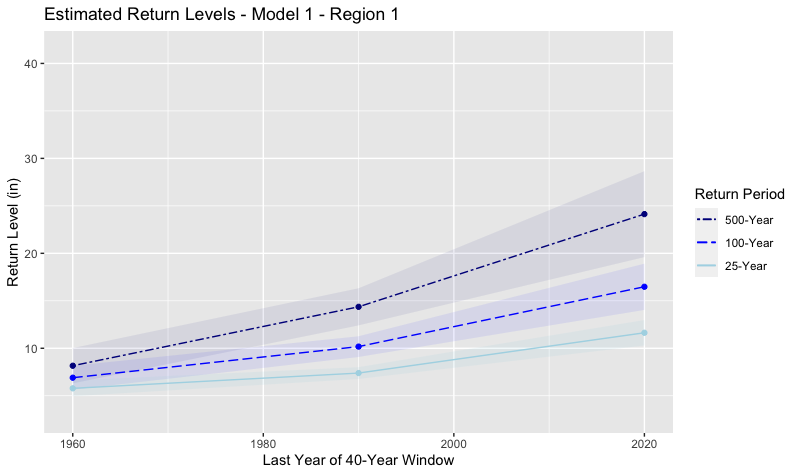
	(a)
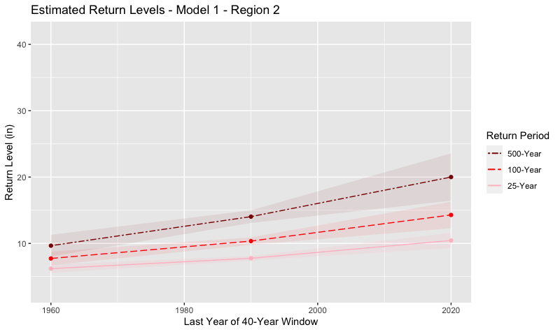
	(b)
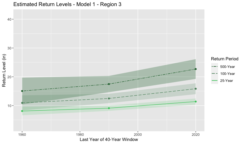
	(c)

Figure 1: Return level estimates and 95% CIs for moving windows - PARE Model

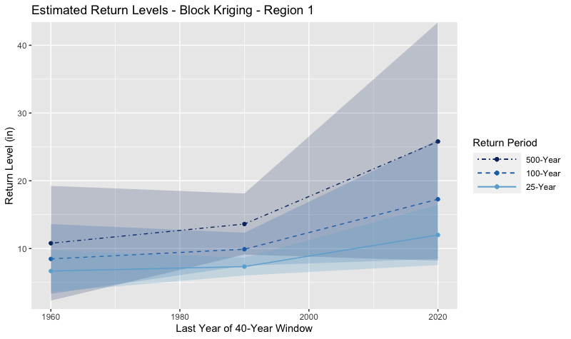
	(a)
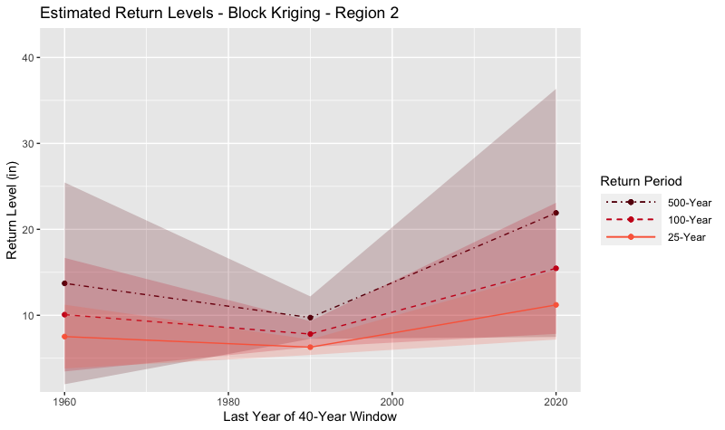
	(b)
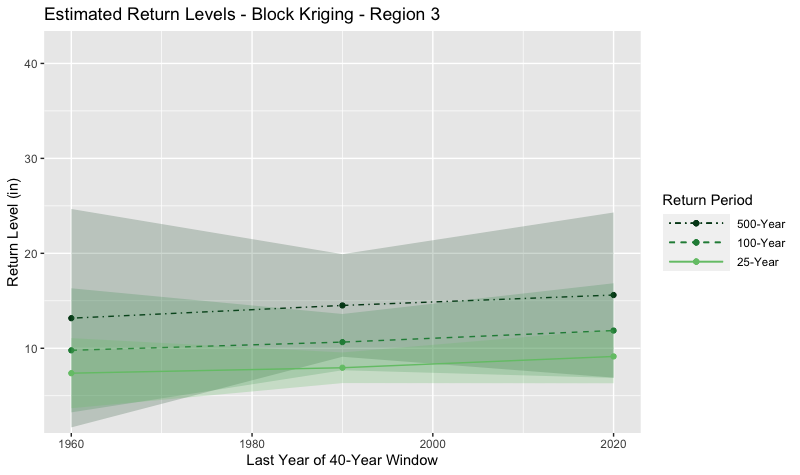
	(c)

Figure 2: Return level estimates and 95% CIs for moving windows - Block Kriging

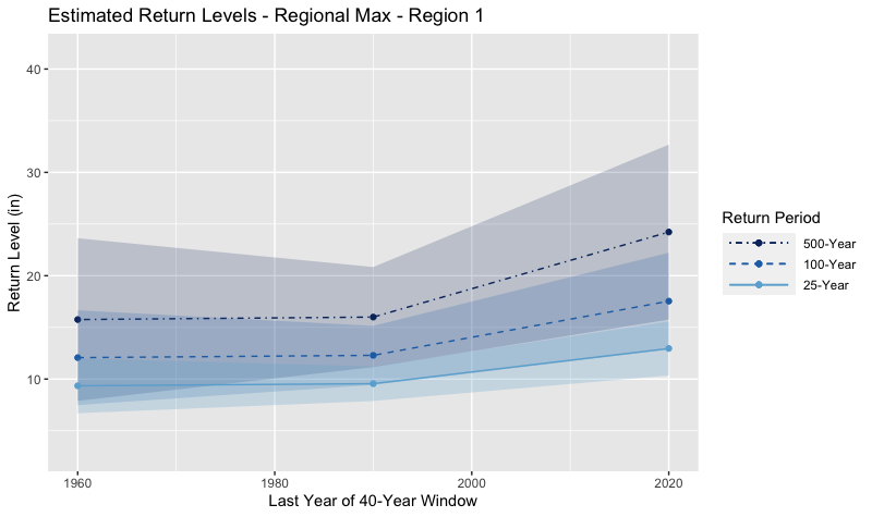
	(a)
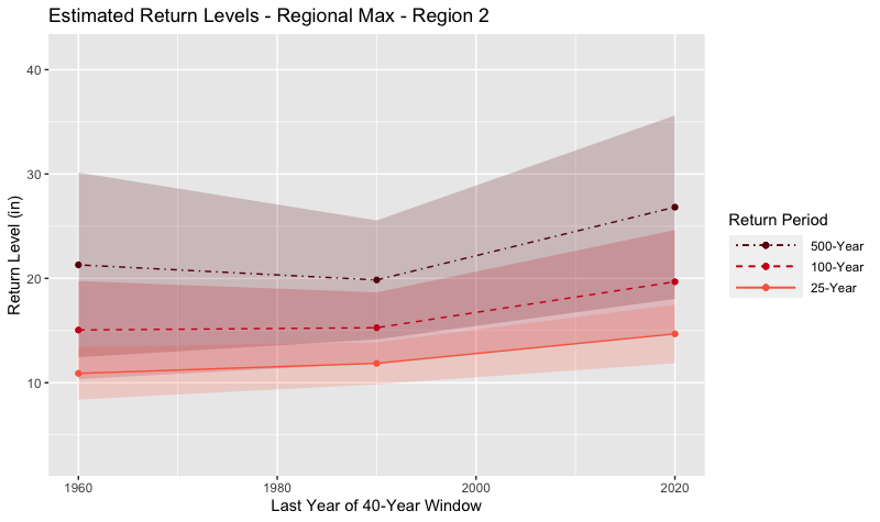
	(b)
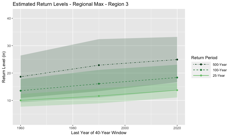
	(c)

Figure 3: Return level estimates and 95% CIs for moving windows - Regional Max

One interesting result is that the return level estimates for the PARE model have fairly narrow confidence intervals. This indicates that the PARE model performs well at providing reliable estimates at the region level. For all regions and return levels, the PARE model has lower uncertainty estimates than the regional max and the block kriging approach. The regional max model in turn has very wide confidence intervals across all windows and regions. Similar to how we suspected the construction of the data using the maximum increases the return level estimates for the regional max model, it also increases the variability of these estimates and therefore the confidence interval widths.

We note that there has been an effort in recent years to update extreme rainfall data in the Houston area. In particular, NOAA Atlas 14 released updated rainfall frequency estimates for all of Texas in 2018 (Perica et al.,, 2018). This updated data set provides gridded precipitation frequency estimates (equivalent to return levels) across Texas for multiple durations (ranging from 5 minutes to 60 days) and multiple return periods (from 1 to 1000 years). We wish to compare our regional return level estimates to updated region estimates for the Harris County hydrologic regions using this updated NOAA Atlas 14 data. As of the time of writing, the only such study found which also aims to bring return level estimates to the region level is a report produced by the American Council of Engineering Companies (ACEC) in Houston in 2019 (ACECHouston,, 2019). The goals of this study slightly differed from ours, as they used the NOAA Atlas 14 frequency estimates directly, and also use these estimates to determine ideal regions for Harris County (i.e. grouping the watersheds into regions themselves). This resulted in almost the same designation as that of the Harris County Flood Control District (HCFCD) manual (Storey and Talbott,, 2009) which we use, except that ACEC placed the Sims Bayou watershed in region 2 as opposed to region 3.

We compare our estimated regional return levels for the last 40-year window (1981-2020) to the ACEC study estimates in Table 8. We note that since regions 2 and 3 were slightly different between our analysis and theirs, we cannot compare these values directly, and so mark them with an asterisk. However, region 1 is designated exactly the same for both studies. We discover that our proposed PARE model matches the ACEC estimates more closely than the other models, indicating that the PARE model run on raw rainfall data performs similarly to the most recent advanced modeling of rainfall frequency estimates by NOAA. It is promising that estimates from our PARE model are consistent with these estimates derived from NOAA Atlas 14, because the NOAA report is the official source of precipitation frequency estimates provided for the U.S. government (Perica et al.,, 2018) and is widely used and accepted.

While it is interesting to compare estimates for the hydrologic regions between the different models on our actual data, we do not know the “true” values for the regions. In order to evaluate the ability of each model to capture the underlying truth at the region level given station data, we also test our models using simulations. The generation of simulated data and results of testing on the simulations are discussed in the next section.

4 Simulations

Recall that the purpose of the models above is to bring information and extreme value modeling from the point-referenced observations to the areal level of the three hydrologic regions in Harris County. In order to test the performance of the models proposed, we simulate multiple data sets of similar spatial structure to run the models on. We simulate data assuming true extreme value parameters at the hydrologic region level.

From these simulated data sets, in which we set the true values for each hydrologic region, we can test how well each model recovers these true values.

In order to construct simulated data, we start from the end with our true values, and work backwards step-by-step to create data that results in the proper structure. The first step taken is to observe the mean structure of the extreme value parameters of the data that we already have. Taking the GPD fits of the last 40 years of data (1981-2020) for the stations within the three hydrologic regions, we find the mean values of the shape and scale parameter estimates by region. We set these as the true parameter values for the regions, and aim to recover similar values when we run our models on the simulated data.

In particular, the simulated rainfall data are generated on a uniform grid with a resolution of three miles. This produces 314 points of daily rainfall data within the three hydrologic regions. The simulation grid is visible in Figure 4. All points falling within a region are assigned the same true shape and scale parameters, which are the average values calculated from the last 40 years of observed data.

For the rate parameter, we decide to simplify the simulation structure and hold this parameter constant. As can be seen in our results of the parameter estimates for the regions in Table 2, the rate parameter has the least deviation between regions or models, staying fairly constant throughout. The constant rate is set to be 0.0544, the observed average of the rate parameter across all stations in the last 40-year period (1981-2020).

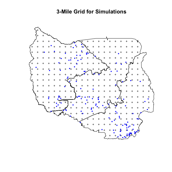
Figure 4: Map of the three hydrologic regions in Harris County (outlined in black), the station locations with data available for the 1981-2020 period (blue dots), and the grid locations where the simulated rainfall data are generated to (+ symbols).

For the next step, we use the parameter estimates at each location to simulate daily rainfall data from the GPD. Since we use the GPD to model independent exceedances above the threshold, we can similarly only generate data values that are independent observations above the threshold. As such, we only generate a proportion of the daily data– a proportion which is equal to our constant rate. For a 40-year period, we generate 795 daily values. We are not able to fully reconstruct real-looking data for the remaining daily observations that fall under the threshold, but fortunately this is not an issue when running our models, because they only work with data above the threshold. In order to preserve the same rate parameter estimates for our fit, we simply fill the remaining daily values with zero or some value below the threshold. This data will give the same GPD fits as a data set that did have the values under the threshold filled in, since the GPD only takes in exceedances over the threshold and the rate of exceedance (percent of observations above the threshold). We generate rainfall values (exceeding the threshold) from the GPD using the revd function from the extRemes package in R (Gilleland and Katz,, 2016).

Note that our generated rainfall data lacks time-reference since we did not assign the data values to specific dates. We can only guarantee that the generated observations are independent. As such, we do not have to worry about declustering the simulated data before fitting to the GPD.

The lack of time-referencing only poses a problem for the regional max model, since it works off of the raw time-referenced daily data and not the GPD fits at the station level. In the interest of evaluating the performance of the regional max model in capturing the true parameter values, we propose an additional step to reorder the simulated rainfall values to impose a psuedo-time-referencing. This approach makes use of the idea that for one day, if there is a large rainfall amount at one station, the other stations are more likely to also have larger rainfall amounts that day than smaller. In general, rainfall totals across stations in a single day will be correlated, though not perfectly. We describe below the process of reordering the simulated rainfall values to impose this idea of daily correlation.

In order to preserve the constant rate, we work only with the data above the threshold, or the 795 rainfall values simulated for each station on our simulation grid. For each of our 314 stations on the grid, we rank the simulated rainfall data from least to greatest. If we were to reorder each station’s data by this ranking, we would have perfect correlation of each station’s smallest rainfall amount occurring on the same day. However, as we mentioned above, this daily correlation is not perfect in reality. In order to offset this perfect correlation and slightly randomize the order of data, we add a uniform random variable between 0–10 to the rankings of the rainfall data. We then re-rank based off of these updated rank values. The data for each station are then reordered, being placed at the “day” the rank indicates. This creates an updated simulated data set that includes all of the same data as before, but has been reordered so that the rainfall values across stations in one row of simulated data can be considered as occurring on the same day. Therefore, the regional max approach can be implemented, taking the maximum across each row based on the region each station falls within.

The steps to generating the simulated data are summarized below. Again, we start with the parameter estimates found through univariate extreme value modeling at each of the stations. We use our real data for the last 40 years to determine true extreme value parameters based on region and use this information to simulate new data with a similar but simplified structure.

Step 1:

Using the stations that fall within each region, calculate the mean parameter values directly or through linear regression with dummy variables.

Step 2:

Generate a uniform grid of points across the three regions to simulate data to.

Step 3:

Assign true parameter values to each simulated data point based on what region the point falls within. All points within the same region will have the same shape and scale parameter values. All points regardless of region will have the same rate parameter, as this is held constant.

Step 4:

Using the assigned parameter values for each location, simulate daily rainfall exceedance data using the revd function in the extRemes package.

Step 5:

Reorder the simulated rainfall data above the threshold in order to impose the concept of time-referenced data with correlated amounts across stations occurring on the same day. (This step is only necessary if testing the regional max model. The other models will give the same output whether or not this step is conducted.)

4.1 Results from Simulation Study

Fifty iterations of the simulation are performed and the results displayed in Table 9. While the first two models both performed well at recovering the true parameter values, our PARE Model performs almost uniformly better than the block kriging model according to the RMSE and MAE. The block kriging model only performed better in estimating the scale parameter for region 3, according to the RMSE. The regional max model performed much worse at capturing the true parameter values, especially that of the scale, just as we expected after seeing the large scale estimates earlier in the results on observed data (see Table 2). The RMSE and MAE values for the regional max were around 10–30 times larger than those of the other two models.

5 Discussion

The PARE method provides robust return level estimates with the least uncertainty when compared with the Block Kriging and Regional Max models. A key advantage of the PARE approach is the use of standard software, ensuring ease of use for future problems. The method also easily incorporates additional fixed effects.

Supplementary Materials

Code to reproduce the PARE analysis for the three windows considered in this paper is provided as a pdf vignette in the supplemental materials. Due to large file sizes, additional resources on the GPD fitting process for all 80 years’ worth of rolling windows and models used for comparison to PARE are provided on Github (Schedler, 2023b, ).

Parameter	Region 1	Region 2	Region 3
scale	208.34 [208.18]	227.62 [227.54]	228.68 [228.73]
shape	0.2199 [0.2205]	0.1776 [0.1771]	0.1109 [0.1121]
rate	0.0559 [0.0559]	0.0554 [0.0554]	0.0557 [0.0557]

Table 1: Comparison of parameter estimates from kriging to a fine grid and averaging the gridded values versus using the shortcut in the gstat package to krige to the polygons of our regions. The latter method’s estimates are in brackets. Note that the estimates are very close, so faster computation times lead us to use the built-in functionality of gstat.

Method	Parameter	Region 1	Region 2	Region 3
1. PARE Model	scale	215.08(4.3232)	236.68(4.8949)	223.99(3.6994)
	shape	0.2(0.0164)	0.16(0.0168)	0.19(0.0134)
	rate	0.06(0.0023)	0.04(0.0023)	0.06(0.0019)
2. Block Kriging	scale	208.83 (16.521)	228.30 (18.557)	229.41 (17.530)
	shape	0.2205 (0.0696)	0.1771 (0.0715)	0.1121 (0.0672)
	rate	0.0559 (0.0058)	0.0554 (0.0058)	0.0557 (0.0057)
3. Regional Max	scale	291.21 (14.897)	343.46 (16.778)	331.38 (16.747)
	shape	0.1523 (0.0377)	0.1397 (0.0355)	0.1351 (0.0366)
	rate	0.0565 (0.0019)	0.0601 (0.0020)	0.0557 (0.0019)

Table 2: Comparison of extreme value parameter estimates (standard errors in parentheses) across our proposed models for the last 40 years of data, 1981-2020. As we predicted, the regional max results differ more than the other two models with its scale parameters being much higher, which may lead to larger return level estimates.

Method	Return Period	Region 1	Region 2	Region 3
1. PARE Model	25-Year	11.634(0.6874)	10.442(0.5857)	11.399(0.5461)
	100-Year	16.48(1.2435)	14.291(1.0239)	15.856(0.9666)
	500-Year	24.131(2.3097)	20.002(1.8186)	22.7(1.7504)
2. Block Kriging	25-Year	12.008 (2.266)	11.210 (2.058)	9.141 (1.443)
	100-Year	17.277 (4.485)	15.465 (3.891)	11.865 (2.545)
	500-Year	25.800 (8.969)	21.911 (7.364)	15.607 (4.437)
3. Regional Max	25-Year	12.959 (1.332)	14.682 (1.435)	13.753 (1.354)
	100-Year	17.541 (2.391)	19.676 (2.531)	18.370 (2.387)
	500-Year	24.227 (4.318)	26.828 (4.484)	24.937 (4.220)

Table 3: Comparison of return level estimates (in inches) across our proposed models for the last 40 years of data, 1981-2020. Standard error estimates are displayed in parentheses.

Method	Parameter	Region 1	Region 2	Region 3
1. PARE Model	scale	230.86(5.3213)	200.16(3.0221)	198.46(4.6)
	shape	-0.02(0.0314)	0.05(0.0205)	0.15(0.0316)
	rate	0.03(6e-04)	0.03(4e-04)	0.03(6e-04)
2. Block Kriging	scale	208.16 (12.248)	194.78 (10.800)	196.99 (12.508)
	shape	0.0720 (0.0946)	0.1382 (0.0925)	0.1274 (0.0976)
	rate	0.0304 (0.0010)	0.0304 (0.0010)	0.0304 (0.0010)
3. Regional Max	scale	247.98 (19.964)	240.98 (14.561)	237.30 (14.690)
	shape	0.1021 (0.0609)	0.1722 (0.0458)	0.1492 (0.0478)
	rate	0.0513 (0.0027)	0.0430 (0.0017)	0.0437 (0.0017)

Table 4: Extreme value parameter estimates (standard errors in parentheses) from our proposed models for the first 40-year window, 1921-1960.

Method	Parameter	Region 1	Region 2	Region 3
1. PARE Model	scale	171.96(4.4827)	202.32(2.7176)	217.8(6.6254)
	shape	0.17(0.0131)	0.13(0.0068)	0.16(0.0153)
	rate	0.03(7e-04)	0.03(3e-04)	0.03(8e-04)
2. Block Kriging	scale	182.43 (8.449)	205.61 (8.644)	203.37 (10.734)
	shape	0.1491 (0.0395)	0.0485 (0.0358)	0.1388 (0.0449)
	rate	0.0306 (0.0009)	0.0320 (0.0009)	0.0327 (0.0010)
3. Regional Max	scale	249.41 (12.471)	318.75 (15.270)	243.09 (13.875)
	shape	0.1007 (0.0361)	0.0964 (0.0338)	0.1775 (0.0444)
	rate	0.0570 (0.0019)	0.0593 (0.0020)	0.0508 (0.0018)

Table 5: Extreme value parameter estimates (standard errors in parentheses) from our proposed models for the second 40-year window, 1951-1990.

Method	Return Period	Region 1	Region 2	Region 3
1. PARE Model	25-Year	5.781(0.4269)	6.2(0.3274)	8.102(0.7539)
	100-Year	6.9(0.645)	7.733(0.5268)	10.938(1.3344)
	500-Year	8.161(0.9508)	9.66(0.8373)	15.059(2.3736)
2. Block Kriging	25-Year	6.681 (1.578)	7.523 (1.895)	7.376 (1.885)
	100-Year	8.472 (2.630)	10.073 (3.372)	9.784 (3.335)
	500-Year	10.789 (4.319)	13.717 (5.990)	13.170 (5.870)
3. Regional Max	25-Year	9.349 (1.354)	10.895 (1.283)	10.037 (1.179)
	100-Year	12.073 (2.341)	15.050 (2.402)	13.553 (2.161)
	500-Year	15.759 (4.016)	21.297 (4.517)	18.659 (3.956)

Table 6: Return level estimates (in inches) from our proposed models for the first 40-year window, 1921-1960. Standard error estimates are displayed in parentheses.

Method	Return Period	Region 1	Region 2	Region 3
1. PARE Model	25-Year	7.391(0.3201)	7.759(0.1733)	9.104(0.4793)
	100-Year	10.177(0.5587)	10.354(0.2883)	12.477(0.8223)
	500-Year	14.367(0.9991)	14.038(0.4891)	17.472(1.4436)
2. Block Kriging	25-Year	7.337 (0.670)	6.289 (0.462)	7.950 (0.823)
	100-Year	9.900 (1.244)	7.818 (0.771)	10.650 (1.511)
	500-Year	13.621 (2.299)	9.728 (1.260)	14.511 (2.757)
3. Regional Max	25-Year	9.552 (0.854)	11.858 (1.025)	11.636 (1.381)
	100-Year	12.295 (1.455)	15.272 (1.730)	16.109 (2.578)
	500-Year	15.999 (2.470)	19.852 (2.909)	22.889 (4.847)

Table 7: Return level estimates (in inches) from our proposed models for the second 40-year window, 1951-1990. Standard error estimates are displayed in parentheses.

Method	Return Period	Region 1	Region 2	Region 3
1. PARE Model	25-Year	11.634(0.6874)	10.442(0.5857)	11.399(0.5461)
	100-Year	16.48(1.2435)	14.291(1.0239)	15.856(0.9666)
	500-Year	24.131(2.3097)	20.002(1.8186)	22.7(1.7504)
2. Block Kriging	25-Year	12.01 (2.27)	11.21 (2.06)	9.14 (1.44)
	100-Year	17.28 (4.48)	15.46 (3.89)	11.87 (2.54)
	500-Year	25.80 (8.97)	21.91 (7.36)	15.61 (4.44)
3. Regional Max	25-Year	12.96 (1.33)	14.68 (1.44)	13.75 (1.35)
	100-Year	17.54 (2.39)	19.68 (2.53)	18.37 (2.39)
	500-Year	24.23 (4.32)	26.83 (4.48)	24.94 (4.22)
ACEC Estimates	25-Year	10.90	11.50*	12.30*
	100-Year	16.30	16.90*	18.00*
	500-Year	24.20	25.00*	27.20*

Table 8: Comparison of return level estimates (in inches) across the proposed models for the last 40 years of data, 1981-2020. Standard error estimates are displayed in parentheses. Additionally, the model estimates are compared to region estimates produced by the American Council of Engineering Companies (ACEC) in Houston (ACECHouston,, 2019). The ACEC estimates for regions 2 and 3 are marked with asterisks because the hydrologic regions are slightly different than the HCFCD designation. Our proposed PARE Model produces very similar estimates to the ACEC study for region 1, which is the same as our region 1.

			Model 1 - PARE Model			Model 2 - Block Kriging			Model 3 - Regional Max
		Truth	Mean	RMSE	MAE	Mean	RMSE	MAE	Mean	RMSE	MAE
Scale	Region 1	233.64	233.96	1.3466	1.0536	235.85	2.5194	2.2470	250.84	17.5993	17.1950
	Region 2	246.78	247.07	1.3125	1.0537	245.11	2.1282	1.8337	264.27	17.8354	17.4853
	Region 3	229.38	229.70	1.1994	0.9160	229.61	1.1697	0.9225	247.01	17.9624	17.6309
Shape	Region 1	0.2044	0.2013	0.0056	0.0044	0.1984	0.0072	0.0065	0.3326	0.1291	0.1282
	Region 2	0.2319	0.2295	0.0050	0.0041	0.2261	0.0073	0.0061	0.3676	0.1363	0.1357
	Region 3	0.1641	0.1621	0.0044	0.0035	0.1700	0.0071	0.0060	0.2775	0.1143	0.1134

Table 9: Extreme value parameter estimates from our proposed models tested on the simulated data for 50 iterations. Note that the rate parameter is held constant, so rate estimates are not evaluated here. Included are the true parameter values used for simulation (Truth), as well as the mean parameter estimates (Mean), root mean squared error (RMSE), and mean absolute error (MAE) for each region and each model from the 50 iterations. Smaller values of RMSE and MAE indicate better performance of a model at recovering the true parameter values. Our proposed PARE Model performs almost uniformly better according to these metrics.

References

- ACECHouston, (2019) ACECHouston (2019). Recommendation for: Rainfall Depths and Intensities in Harris County. Technical Report, ACEC Houston.
- Besag, (1974) Besag, J. (1974). Spatial Interaction and the Statistical Analysis of Lattice Systems. Journal of the Royal Statistical Society. Series B (Methodological), 36(2):192–236. Publisher: [Royal Statistical Society, Wiley].
- Bivand et al., (2013) Bivand, R. S., Pebesma, E., and Gómez-Rubio, V. (2013). Applied Spatial Data Analysis with R. UseR! Series. Springer, 2nd edition.
- Cooley et al., (2012) Cooley, D., Cisewski, J., Erhardt, R. J., Mannshardt, E., Jeon, S., Omolo, B. O., and Sun, Y. (2012). A Survey of Spatial Extremes : Measuring Spatial Dependence and Modeling Spatial Effects. REVSTAT-Statistical Journal, 10(1):135–165. Number: 1.
- Craigmile, (2014) Craigmile, P. F. (2014). Spatial change-of-support and misalignment problems.
- Cressie, (2006) Cressie, N. (2006). Block Kriging for Lognormal Spatial Processes. Mathematical Geology, 38(4):413–443.
- Cressie and Wikle, (2011) Cressie, N. and Wikle, C. K. (2011). Statistics for Spatio-Temporal Data. John D. Wiley & Sons, Inc., Hoboken, NJ.
- Darling, (1957) Darling, D. A. (1957). The Kolmogorov-Smirnov, Cramer-von Mises Tests. The Annals of Mathematical Statistics, 28(4):823–838. Publisher: Institute of Mathematical Statistics.
- Fagnant, (2021) Fagnant, C. (2021). Spatiotemporal Extreme Value Modeling with Environmental Applications. Thesis, Rice University. Accepted: 2021-10-06T16:17:51Z.
- Fagnant et al., (2020) Fagnant, C., Gori, A., Sebastian, A., Bedient, P. B., and Ensor, K. B. (2020). Characterizing spatiotemporal trends in extreme precipitation in Southeast Texas. Natural Hazards, 104(2):1597–1621.
- Gelfand et al., (2001) Gelfand, A. E., Zhu, L., and Carlin, B. P. (2001). On the change of support problem for spatio-temporal data. Biostatistics, 2(1):31–45.
- Getis, (2009) Getis, A. (2009). Spatial Weights Matrices. Geographical Analysis, 41(4):404–410. _eprint: https://onlinelibrary.wiley.com/doi/pdf/10.1111/j.1538-4632.2009.00768.x.
- Getis and Aldstadt, (2004) Getis, A. and Aldstadt, J. (2004). Constructing the Spatial Weights Matrix Using a Local Statistic. Geographical Analysis, 36(2):90–104. _eprint: https://onlinelibrary.wiley.com/doi/pdf/10.1111/j.1538-4632.2004.tb01127.x.
- Gilleland and Katz, (2016) Gilleland, E. and Katz, R. W. (2016). extRemes 2.0: An Extreme Value Analysis Package in R. Journal of Statistical Software, 72:1–39.
- Gotway and Young, (2002) Gotway, C. A. and Young, L. J. (2002). Combining Incompatible Spatial Data. Journal of the American Statistical Association, 97(458):632–648. Publisher: [American Statistical Association, Taylor & Francis, Ltd.].
- Miranda et al., (2021) Miranda, M. L., Callender, R., Canales, J. M., Craft, E., Ensor, K. B., Grossman, M., Hopkins, L., Johnston, J., Shah, U., and Tootoo, J. (2021). The Texas flood registry: a flexible tool for environmental and public health practitioners and researchers. Journal of Exposure Science & Environmental Epidemiology, 31(5):823–831. Number: 5 Publisher: Nature Publishing Group.
- Pebesma, (2004) Pebesma, E. J. (2004). Multivariable geostatistics in S: the gstat package. Computers & Geosciences, 30(7):683–691.
- Perica et al., (2018) Perica, S., St. Laurent, M., Trypaluk, C., Unruh, D., and Wilhite, O. (2018). Precipitation-Frequency Atlas of the United States. Volume 11, Version 2.0. Texas. Publisher: United States, National Weather Service.
- Schedler, (2020) Schedler, J. C. (2020). Advances in the Analysis of Spatially Aggregated Data. Thesis, Rice University. Accepted: 2020-04-27T19:14:17Z.
- (20) Schedler, J. C. (2023a). juliaSchedler/hausdorff. original-date: 2023-07-27T18:45:52Z.
- (21) Schedler, J. C. (2023b). juliaSchedler/ST_pare. original-date: 2023-07-31T16:13:11Z.
- Storey and Talbott, (2009) Storey, A. and Talbott, M. (2009). Harris County Flood Control District Hydrology and Hydraulics Guidance Manual. Technical Report.