Revealing Impact of Critical Stellar Central Density on Galaxy Quenching through Cosmic Time

Abstract

In the previous work of Xu & Peng (2021), we investigated the structural and environmental dependence on quenching in the nearby universe. In this work we extend our investigations to higher redshifts by combining galaxies from SDSS and ZFOURGE surveys. In low density, we find a characteristic $\Sigma_{1\ kpc}$ above which the quenching is initiated as indicated by their population-averaged color. $\Sigma^{crit}_{1\ kpc}$ shows only weakly mass-dependency at all redshifts, which suggests that the internal quenching process is more related to the physics that acts in the central region of galaxies. In high density, $\Sigma^{crit}_{1\ kpc}$ for galaxies at $z>1$ is almost indistinguishable with their low-density counterparts. At $z<1$, $\Sigma^{crit}_{1\ kpc}$ for low-mass galaxies becomes progressively strongly mass-dependent, which is due to the increasingly stronger environmental effects at lower redshifts. $\Sigma^{crit}_{1\ kpc}$ in low density shows strong redshift evolution with $\sim 1$ dex decrement from $z=2.5$ to $z=0$. It is likely due to that at a given stellar mass, the host halo is on average more massive and gas-rich at higher redshifts, hence a higher level of integrated energy from more massive black hole is required to quench. As the halo evolves from cold to hot accretion phase at lower redshifts, the gas is shock-heated and becomes more vulnerable to AGN feedback processes, as predicted by theory. Meanwhile, angular momentum quenching also becomes more effective at low redshifts, which complements a lower level of integrated energy from black hole to quench.

1 Introduction

One of the long-standing puzzles of galaxy evolution is to understand how and why the star-forming activity in galaxies is seized (“quenched”). The processes to quench the star formation can be broadly classified into two categories (Kauffmann & Heckman, 2003; Baldry et al., 2006; Peng et al., 2010): internally driven processes, named as “mass quenching” that operates in both central and satellite galaxies; and externally driven processes, known as “environment quenching” which only operates in satellite galaxies. Various mechanisms have been proposed to account for the underlying physics. For mass quenching, the candidate mechanisms include AGN feedback (Croton et al., 2006; Darvish et al., 2015, 2016; Lin et al., 2016; De Lucia et al., 2019), morphological quenching (Martig et al., 2009), gravitational quenching (Genzel et al., 2014), and angular momentum quenching (Peng & Renzini, 2020; Renzini, 2020). Mechanisms for environment quenching consist of strangulation (Balogh et al., 1997) , ram-pressure stripping (Gunn & Gott, 1972; Abadi et al., 1999), tidal interaction (Sobral et al., 2011), and halo quenching (Dekel & Birnboim, 2006). Despite equipped with various options, a definitive concensus on which processes contribute to what extent is still lacking.

Attempts to push our understanding of quenching forward have been extensively made in investigating the correlations between various physical parameters and the quiescence of galaxies. Studies of massive galaxies suggest that the surface mass density within the central radius of 1 kpc ($\Sigma_{1\ kpc}$) is strongly correlated with the quenched fraction of galaxies, hence can be treated as an effective probe to quenching. The usage of $\Sigma_{1\ kpc}$ was first reported in Cheung et al. (2012), who found that high $\Sigma_{1\ kpc}$ performs best in predicting quenching at $z\sim 0.7$. Fang et al. (2013) found that for nearby Sloan Digital Sky Survey (SDSS) galaxies, specific star formation rate (sSFR) varies systematically relative to $\Sigma_{1\ kpc}$, suggesting a mass-dependent threshold of $\Sigma_{1\ kpc}$ for the onset of quenching, possibly due to a threshold in black hole mass. van Dokkum et al. (2014); Tacchella et al. (2015); Barro et al. (2017) extended the use of $\Sigma_{1\ kpc}$ as a predictor of quenching to galaxies at higher redshifts. Whitaker et al. (2017) studied the population-averaged sSFR as a function of $\Sigma_{1\ kpc}$ for galaxies at $0.5<z<2.5$, and found a sharp decrease in sSFR as $\Sigma_{1\ kpc}$ exceeds some threshold. They also found that the critical $\Sigma_{1\ kpc}$ has strong redshift evolution. Chen et al. (2020) proposed an analytic model to explain the quenching boundaries as a competition of halo binding energy with the integrate power of AGN feedback. Luo et al. (2020) found that the offset to the running median of $\Sigma_{1\ kpc}$ has the power of distinguishing the bulge types in nearby galaxies. More recently, Xu & Peng (2021) use a sample of nearby SDSS galaxies to study the distribution of population-averaged (NUV - r) color on the $M_{\star}-\Sigma_{1\ kpc}$ plane, and its environmental dependence. They found that for central galaxies in low density, there exists a critical central density $\rm\Sigma^{crit}_{1\ kpc}\sim 10^{9}-10^{9.2}M_{\odot}\,kpc^{-2}$, above which the quenching initiates. Intriguingly, this $\Sigma^{crit}_{1\ kpc}$ is only weakly dependent on the stellar mass.

Surprisingly, $\Sigma_{1\ kpc}$ appears also correlated with the quiescence of satellite galaxies. Woo et al. (2017) showed that $\Sigma_{1\ kpc}$ in quenched satellites is $\sim 0.3$ dex higher than that of star-forming satellites at fixed stellar mass. Kawinwanichakij et al. (2017); Guo et al. (2021) reach similar conclusions for satellites at high redshifts. Xu & Peng (2021) find that the critical $\Sigma_{1\ kpc}$ at the transition from star-forming to passive populations is strongly mass-dependent for low-mass satellites. Moreover, they found that the mass-dependence in $\Sigma^{crit}_{1\ kpc}$ for low-mass satellites is a function of environment: $\Sigma^{crit}_{1\ kpc}$ is lower in dense environment, at fixed stellar mass.

To gain further insight of the underlying physics of quenching, a natural logic is to extend the work of Xu & Peng (2021) to higher redshifts, to study the redshift evolution of the structural and environmental impacts on quenching, which is the goal of this paper. In this work, we utilize the samples of galaxies from Sloan Digital Sky Survey (SDSS) and The FourStar Galaxy Evolution (ZFOURGE) surveys to perform a joint analysis on the structural and environmental dependence on quenching at $0<z<2.5$. Photometric redshift based on broad-band photometry with large uncertainty is the main obstacle to study the galaxy environment at high redshifts. ZFOURGE survey utilize five near-IR medium-band filters to better constrain the photometric redshift, which enables more precise characterization of the environment at high redshifts. Throughout, we adopt the following cosmological parameters where appropriate: $H_{0}$ = 70 km $s^{-1}$Mpc^-1, $\Omega_{m}$ = 0.3, and $\Omega_{\lambda}$ = 0.7.

2 Data and Analysis

2.1 The nearby galaxies

In this work, we use the same sample of nearby galaxy as used in Xu & Peng (2021), which was constructed from Sloan Digital Sky Survey (SDSS) DR7 catalog (Abazajian et al., 2009). The redshift range is $0.02<z<0.085$, which guarantees reliable spectroscopic redshift measurements. Each galaxy is weighted by 1/TSR $\times$ 1/V_max , where TSR is the spatial target sampling rate, determined using the fraction of objects that have spectra in the parent photometric sample within the minimum SDSS fiber spacing of 55” of a given object. The V_max values are derived from the $k$-correction program version 4.2 (Blanton & Roweis, 2007). The use of V_max weighting allows us to correct the effect of incompleteness of the sample down to a stellar mass of about $10^{9}\ M_{\odot}$.

Integrated photometries in five bands were used in this study: $u,g,r,i,z$ bands from SDSS. The photometries were corrected for Galactic extinction and $k$-weighted to $z=0$ using version 4.2 of the $k$-correct code package described in Blanton & Roweis (2007). The spectroscopic redshifts, total stellar mass, fiber velocity dispersion, and median signal-to-noise ratios (S/Ns) in the spectra were obtained from the MPA/JHU DR7 value-added catalog. The stellar masses were computed by fitting the integrated SDSS photometry with the stellar population models (similar to the method in Salim et al. (2007)). The structural parameters such as Sersic index $n$, effective radius $R_{e}$, ellipticity $e$ are obtained from (Simard et al., 2011). The axis ratio is computed as $b/a=1-e$ as defined.

2.2 The galaxies at high redshift

We select galaxies at $0.5<z<2.5$ from The FourStar Galaxy Evolution (ZFOURGE) survey (Straatman et al., 2016). The survey is composed of three 11’ $\times$ 11’ fields with coverage in the regions of CDFS (Giacconi et al., 2002), COSMOS (Scoville et al., 2007), and UDS (Lawrence et al., 2007) that overlap with the Cosmic Assembly Near-IR Deep Extragalactic Legacy Survey (CANDELS; Grogin et al. (2011); Koekemoer et al. (2011)), which also provide Hubble Space Telescope (HST), high-angular resolution imaging for 0.6 - 1.6 $\mu$m (see, e.g., van der Wel et al. (2012)). ZFOURGE utilize five near-IR medium-bandwidth filter: $J_{1}$, $J_{2}$, $J_{3}$, $H_{s}$ and $H_{l}$ to better constrain the photometric redshift. The medium-band near-IR imaging in $J_{1}$, $J_{2}$, $J_{3}$ reaches depths of $\sim 26$ AB mag and $\sim$ 25 AB mag in $H_{s}$ and $H_{l}$. We utilize ZFOURGE main catalogs which are provided by the official ZFOURGE website. The main catalogs are complete for galaxies to $K_{s}\sim 25.5-26.0$ AB mag (see Straatman et al. (2016)), and include photometric redshifts and rest-frame colors calculated using EAZY (Brammer et al., 2008) from 0.3 to 8 $\mu$m photometry for each galaxy. The typical photometric-redshift uncertainties are $\sigma_{z}/(1+z)$ = 0.01-0.02 to the $K_{s}$-band magnitude limit for galaxies between $z=0.5$ and $z=2.0$, with negligible dependence on galaxy color (Straatman et al., 2016). In addition, the morphological data that are cross-matched with Hubble Space Telescope (HST)/WFC3/F160W CANDELS data from van der Wel et al. (2012) are also included.

2.3 Sample selections

We select the nearby galaxies above the SDSS spectroscopic limit ($r=17.77$) and with the stellar mass log$(M_{\star}/M_{\odot})>9$. We discard galaxies with low axis ratio with $b/a<0.5$ to minimize the measurement bias due to the internal dust extinction. A final sample of 89,469 nearby galaxies is produced for the subsequent analysis.

For galaxies at high redshifts, we first select all the well-detected galaxies (‘USE’ flag = 1) with the stellar mass log$(M_{\star}/M_{\odot})>9$; we then discard galaxies with $H$-band magnitude fainter than 24.5 AB mag to guarantee an accurate structural measurement (van der Wel et al., 2012). To see if this additional magnitude cut of $H<24.5$ AB mag has any impact on the original stellar mass completeness determined based on the limit of $K_{s}\sim 25.5-26.0$ AB mag (Kawinwanichakij et al., 2017), we compute the fraction of galaxies that have both $H<24.5$ and $K_{s}<25.5$ to the galaxies that have $K_{s}<25.5$ only to evaluate the impact of the cut $H<24.5$ (see Table 1). The fraction is higher than $97\%$ at all redshifts, which indicates that the additional cut on H-band will not affect the level of completeness of the sample.

$z$		$\frac{N_{g}(H<24.5\,\&\,K_{s}<25.5)}{N_{g}(K_{s}<25.5)}$
$0.5<z<1.0$		99.31%
$1.0<z<1.5$		99.10%
$1.5<z<2.0$		99.45%
$2.0<z<2.5$		97.45%

Table 1: Fraction of galaxies that satisfy both $H<24.5$ and $K_{s}<25.5$ to the galaxies that have $K_{s}<25.5$ only, at four redshift bins.

Similarly, we discard galaxies from ZFOURGE catalog with axis ratio $b/a<0.5$ to ensure a reliable measurement of Sersic index $n$ and $R_{e}$. In addition, we use the quality flag to further exclude galaxies with bad GALFIT fitting in F160W band (flag $>$ 1). A final sample of 4,577 galaxies at $0.5<z<2.5$ makes the cut.

2.4 The Central 1kpc Mass Density

We follow the procedures in Xu & Peng (2021) to compute the central 1kpc surface mass density $\Sigma_{\rm 1\ kpc}$, by directly integrating the Sersic light profile and scaling the integrated luminosity within the inner 1 kpc. This method has been widely used in many previous studies (Bezanson et al., 2009; Whitaker et al., 2017; Kawinwanichakij et al., 2017) and is described as follows. The two-dimensional Sersic light profile can be described in the form of

$$I(r)=I_{0}{\rm exp}\left[-b_{n}\left(\frac{r}{r_{e}}\right)^{1/n}\right],$$ (1)

where $I_{0}$ is the central intensity, $n$ is the Sersic indices, $r_{\rm eff}$ is the circularized effective radii, and $b_{n}$ is defined as (Ciotti & Bertin, 1999):

$$b_{n}\approx 2n-\frac{1}{3}+\frac{4}{405n}+\frac{46}{25515n^{2}}.$$ (2)

For the disk galaxies with Sersic indices $n<2.5$ (Kennedy et al., 2015), the total luminosity is obtained by integrating over the two-dimensional light profile (Equation 1). We then convert the total luminosity to the total stellar mass, assuming that the mass follows the light and that there are no strong color gradients. Finally, we calculate the stellar mass surface density in the inner 1 kpc by numerically integrating the following equation:

$$\Sigma_{\rm 1\ kpc}=\frac{\int_{0}^{\rm 1\ kpc}I(r)rdr}{\int_{0}^{\infty}I(r)rdr}\frac{L_{model}}{L_{phot}}\frac{M_{\star}}{\pi(\rm 1\ kpc)^{2}},\quad n<2.5$$ (3)

where $\rm M_{\star}$ is the total stellar mass of the galaxy from the MPA/JHU DR7 value-added catalog for nearby galaxies, and from the ZFOURGE main catalogs for galaxies at high redshifts; $L_{model}$ is the total luminosity from the Sersic modeling, whereas $L_{phot}$ is the measured total luminosity within the aperture. There is only slight difference $\sim$ 0.1 dex between $L_{model}$ and $L_{phot}$(Whitaker et al., 2017; Kawinwanichakij et al., 2017), and we do not include this correction and set $L_{model}/L_{phot}=1$ in this study, to maintain consistency of the computed $\Sigma_{\rm 1\ kpc}$ in nearby and distant galaxies. For galaxies that have prominent bulge components with $n>2.5$, we assume that they follow spherical light profiles and perform an Abel transform to deproject the circularized, three-dimensional light profile (Bezanson et al., 2009):

$$\rho\left(\frac{r}{r_{e}}\right)=\frac{b_{n}}{\pi}\frac{I_{0}}{r_{e}}\left(\frac{r}{r_{e}}\right)^{1/n-1}\times\int_{1}^{\infty}\frac{{\rm exp}[-b_{n}(r/r_{e})^{1/n}t]}{\sqrt{t^{2n}-1}}dt.$$ (4)

The total luminosity in this case is derived by integrating over the above three-dimensional light profile, and the central surface mass density is given as

$$\Sigma_{\rm 1\ kpc}=\frac{\int_{0}^{\rm 1\ kpc}\rho(r)r^{2}dr}{\int_{0}^{\infty}\rho(r)r^{2}dr}\frac{M_{\star}}{\pi(\rm 1\ kpc)^{2}},\quad n>2.5.$$ (5)

For each galaxy, we perturb the stellar mass $M_{\star}$, Sersic index $n$ and size $R_{e}$ within their quoted 1$\sigma$ error for 40 times and compute the corresponding $\Sigma_{1\ kpc}$. The uncertainty of $\Sigma_{1\ kpc}$ is evaluated as the standard deviation of the 40 perturbed $\Sigma_{1\ kpc}$.

2.5 Characterization of Galaxy Environment

Most methods to define and compute the environment of galaxies fall into two categories: those that use flexible apertures whose size is determined by the method of nearest neighbour, and those that use fixed apertures. The choice is largely dependent on the scale being probed: the local environment that is internal to a halo is found to be best measured with the nearest neighbour method; whereas the fixed apertures best quantify the large-scale environment external to a halo (Muldrew et al., 2012). In this study, we characterize the environment of galaxies in local and distant universe by their local projected overdensity using the distance to the $N$th nearest neighbour. The dimensionless overdensity 1 + $\delta$ is defined as Peng et al. (2012):

$$(1+\delta)_{5}=1+\frac{\Sigma_{5}-\langle\Sigma\rangle}{\langle\Sigma\rangle}.$$ (6)

Since there is no physical constraints on the number $N$ yet, the choice of $N$ typically varies from 3 to 10, which largely depends on the surveys (Muldrew et al., 2012; Peng et al., 2012; Kawinwanichakij et al., 2017). For nearby galaxies from SDSS, we adopt $N=5$ and the overdensity is computed from the volume of the cylinder that centered on each galaxy with a length $\pm$1000 $\rm kms^{-1}$. All the five closest neighbor galaxies have $M_{B,AB}\leq-19.3-z$, where $-z$ is used to approximate the luminosity evolution of both passive and active galaxies. For galaxies at high redshift, since the sample with available spectroscopic redshift is very limited, the photometric redshift with larger uncertainty is used to characterize the environment at high redshifts. We adopt an empirical approach to optimize $N$ and the redshift interval $\delta z$ (or the length of the cylinder that centered on each galaxy), which are vital to determine the overdensity. We use $N=8$ and $\delta z=0.08$ in this study. The detail of the precedures can be found in Appendix A.

2.6 Star-forming Indicator

We use (U - V) color as the indicator of star formation in this study, as is widely used in literatures. The rest-frame flux in U and V bands were computed by SED fitting and provided in ZFOURGE “REST-FRAME” catalogs. For nearby SDSS galaxies, Blanton & Roweis (2007) provided sets of empirical formula in their Table 2 to convert $u,g,r$ photometries to U and V magnitudes, which is given as

$$U=u-0.0682-0.0140[(u-g)-1.2638]$$ (7)

$$V=g-0.3516-0.7585[(g-r)-0.6102].$$

We use Eqn 7 to convert the SDSS photometries to rest-frame (U - V) color to be in line with the high-redshift galaxies. The provided color dispersion of $\sigma[u-g]=0.26$ and $\sigma[g-r]=0.15$ were used to estimated the uncertainty of the converted (U - V) color.

2.7 Dust Extinction Correction

Massive dusty galaxies with intense star-forming activity at high redshifts typically show red color, which makes them indistinguishable with passive galaxies based only on (U - V) color. In literatures, UVJ diagram is widely used to effectively break this color degeneracy (Williams et al., 2010), and classify galaxies as star-forming galaxies (SFGs) and quiescent galaxies (QGs). However, a continuous measurement of level of star formation, instead of a dichotomy of galaxies suits this study more. Therefore, we attempt to assume a Calzetti law to correct the rest-frame (U - V) color for the effect of dust extinction. For galaxies at high redshifts, $A_{V}$ is computed from SED fitting and is provided in the ZFOURGE main catalogs. The value of $R_{V}=A_{V}/E(B-V)$ depends on the interstellar environment along the line of sight. In galactic diffuse regions, $R_{V}$ typically has an average value of 3.1 (Draine et al., 2003); whereas in dense molecular clouds, $R_{V}$ could be as large as $\sim 6$ (Mathis et al., 1990; Fitzpatrick, 1999), and it could be as $\sim 2$ in low density region (Fitzpatrick, 1999). A detailed evaluation of $R_{V}$ for different types of galaxies in our sample is definitely beyond the scope of this paper. Instead, we adopt an empirical methodology to “optimize” the value of $R_{V}$ to be in line with the classification based on the UVJ diagram. Overall, the classification based on the corrected (U - V) color best matches that on UVJ diagram when $R_{V}\sim 5.1$ (see details in Appendix B), and we adopt this value of $R_{V}$ to correct the (U - V) color. For nearby SDSS galaxies, $A_{V}$ for each galaxy is obtained by corss-matching our SDSS sample with the Galaxy Evolution Explorer (GALEX)-SDSS-Wide-field Infrared Survey Explorer (WISE) LEGACY CATALOG (GSWLC, Salim et al., 2007). To maintain consistency with galaxies at high redshifts, we use the same value of $R_{V}\sim 5.1$ to correct the (U - V) color.

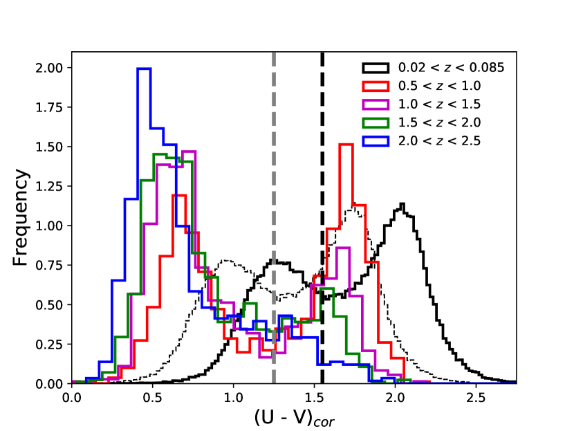
Figure 1: Distribution of dust-extinction corrected rest-frame (U - V) color at five redshift bins. Galaxies are selected with stellar mass $\rm log(M_{\star}/M_{\odot})>9.8$ to guarantee the completeness up to $z\sim 2.5$ (Kawinwanichakij et al., 2017). Color bimodality can be observed at almost all the redshit bins except for the highest one at $2.0<z<2.5$. The gray dashed line marks the color criteria that separates the star-forming and passive populations for galaxies at high redshifts, which is (U - V)${}_{cor}\sim 1.25$. This color criteria is insensitive to the redshift and the level of completeness of the sample. The black dashed line marks the position of color trough that separates two peaks for SDSS galaxies, which is at $\sim$ 1.55. To better visualize the comparison between nearby and distant galaxies, we narrow down the color range of the whole sample by shifting the color distribution of SDSS galaxies by 0.3 dex towards the left (thin dashed line), to align the color trough of SDSS galaxies with those of galaxies at high redshifts. This shifting will not affect the determination of $\Sigma^{crit}_{1\ kpc}$, since the color criteria used in computing $\Sigma^{crit}_{1\ kpc}$ shifts for the same amount as for the whole distribution.

Figure 1 shows the comparison of the distribution of the dust-extinction corrected (U - V) color at $0<z<2.5$. Only galaxies with $\rm log(M_{\star}/M_{\odot})>9.8$ are selected to maintain the completeness level of the sample up to $z\sim 2.5$. Overall, the color of galaxies becomes redder as the redshift decreases. The color bimodality can be clearly observed at almost all the redshifts except for highest redshift bin at $2<z<2.5$. For galaxies at $z>0.5$, the postion of the trough between two peaks is (U - V)_cor $\sim$ 1.25, and does not show significant redshift evolution. The color at $z\sim 0$ is $\sim$ 0.3 - 0.7 dex redder than those at $z>0.5$, which is consistent with the previous result in which the rest-frame (U - V) color was directly derived from SED fitting (Bell et al., 2012). To better visualize the color distribution in galaxies at high redshifts and compare with that of the nearby galaxies, we narrow down the color range of the whole sample by shifting the color distribution of SDSS galaxies by $\sim$ 0.3 dex towards the left in Figure 1 (black dashed line), to align the color trough of SDSS galaxies with those of galaxies at high redshifts. This shifting will not affect the subsequent determination of the critical $\Sigma_{1\ kpc}$, which only depends on the relative position of the trough within the distribution.

In addition, we test if this color criteria is sensitive to the level of completeness of the sample. We repeatedly adjust the lower bound of stellar mass of the sample and re-plot the color distribution, and found the location of the trough remains similar. Therefore, we use (U - V)${}_{cor}\sim 1.25$ as a color criteria for the subsequent analysis.

3 The Structural and Environmental impact on quenching

In this section, we study the structural and environmental impacts on quenching for galaxies at $0<z<2.5$ by investigating the color distribution on the $\rm M_{\star}-\Sigma_{1\ kpc}$ plane. We assign galaxies into five redshift bins to study their redshift evolution. To reveal their environmental dependence, we divide the galaxies in each redshift bin into three envrionment bins based on their rank in local overdensity. For each SDSS galaxy, we perform a $V_{max}$-weighting correction to correct for the incompleteness, inside a box of 0.3$\times$0.2 dex² that centers on each data point. We further smooth the data using the locally weighted regression method LOESS (Cleveland & Devlin, 1988) as implemented by Cappellari et al. (2013). LOESS is useful in unveiling the overall underlying trends by reducing the intrinsic and observational errors, in particular in bins where the number of galaxies is small.

Similar to the approaches in Xu & Peng (2021), we focus on the structural dependence on quenching by quantitatively sketching the trends in $\Sigma_{1\ kpc}$ at the transition from star-forming to passive populations, which is $(U-V)_{cor}\sim 1.25$ in this study, as discussed in Sec 2.7 (also see Figure 1). Figure 2 shows the central 1kpc density $\Sigma_{1\ kpc}$ as a function of stellar mass M_⋆ in three environmental bins and five redshift bins, color-coded by LOESS-smoothed, dust-extinction corrected color (U - V)_cor. In each bin, we select data at the transition that have $1.25-0.15<(U-V)_{cor}<1.25+0.15$ and $\Sigma^{crit}_{1\ kpc}$ is computed as the running median of their $\Sigma_{1\ kpc}$ as a function of stellar mass. We overplot the transitional $\Sigma_{1\ kpc}$ as the magenta dashed lines in Figure 2 for reference. The (U - V)_cor for SDSS galaxies in Figure 2 is 0.3 dex lower than their original value as mentioned in Section 2.7. We replot all galaxies with their original color in Figure 9 in Appendix C. $\Sigma^{crit}_{1\ kpc}$ for SDSS galaxies remains unchanged under the shifting in color space, as expected.

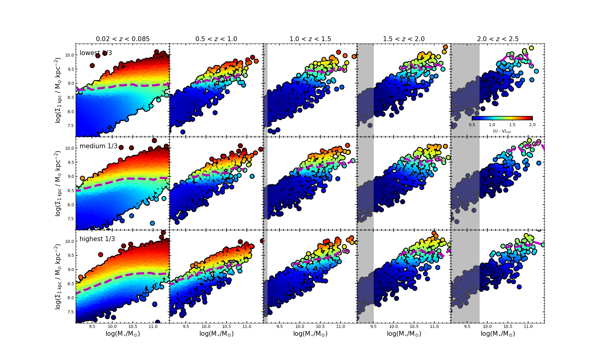
Figure 2: Central 1kpc surface mass density $\Sigma_{1\ kpc}$ as a function of stellar mass at five redshift bins (different columns) and three environment bins (different rows), color-coded by the dust-corrected rest-frame (U - V) color. For the SDSS spectroscopic sample, the data at $0.02<z<0.085$ has been $V_{max}$-weighted; for the ZFOURGE photometric sample at $z>0.5$, the gray shaded region marks the range of stellar mass which is incomplete. The data in each bin has been LOESS smoothed. The magenta dahsed lines denote the transitional $\Sigma_{1\ kpc}$ at (U - V)_cor $\sim$ 1.25.

Overall, there is strong redshift evolution in (U - V)_cor color. At fixed stellar mass, the color at high redshifts is typically bluer than their low redshift counterparts. The critical $\Sigma_{1\ kpc}$ for massive galaxies strongly evolves with redshift that the boundary appears higher at high redshifts. At high redshift ($z>1$), there is no significant difference in $\Sigma^{crit}_{1\ kpc}$ for massive galaxies in different environments; whereas the transitional line becomes environment-dependent at low redshift ($z<1$), in particular for low-mass galaxies.

We highlight these trends in Figure 3 by plotting $\Sigma^{crit}_{1\ kpc}$ as a function of stellar mass in different environments at five redshift bins. The uncertainty of $\Sigma^{crit}_{1\ kpc}$ is estimated by Monte Carlo simulations. In each environment and redshift bin, we create 40 realizations of simulated data by perturbing various parameters. For nearby SDSS galaxies, we add a Gaussian random noise to the observed stellar mass and $\Sigma_{1\ kpc}$, with 1$\sigma$ uncertainty that is equal to their quoted errors. We also perturb the (U - V) color by adding noise to SDSS (u - g) and (g - r) colors with the quoted 1$\sigma$ error (Blanton & Roweis, 2007), and then propogating the errors using Equation 7. For ZFOURGE galaxies, we perturb their stellar mass, $\Sigma_{1\ kpc}$ and photometric redshift by adding a Guassian random noise with their quoted 1$\sigma$ errors, we then rebin the simulated data based on their perturbed redshift and re-calculate the local overdensity in each realization, to account for the uncertainty in the photometric redshift. The colored shades in Figure 3 are the running median and 1$\sigma$ dispersion in $\Sigma^{crit}_{1\ kpc}$.

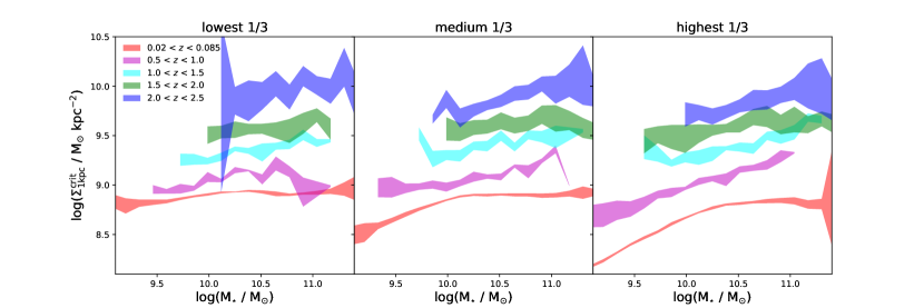
Figure 3: $\Sigma^{crit}_{1\ kpc}$ as a function of stellar mass at five redshift bins and three environment bins. The color-shaded region marks the 1$\sigma$ error of the critical line which is computed by averaging over lines in 40 Monte-carlo simulated realizations in each redshift and environment bin.

The structural and environmental dependence on quenching and their evolution can be clearly depicted in Figure 3. At $z>1$, no clear environmental dependence has been detected in $\Sigma^{crit}_{1\ kpc}$, and $\Sigma^{crit}_{1\ kpc}$ in all environments appears to be flat and exhibits only weak mass-dependency. The mass-dependence of $\Sigma^{crit}_{1\ kpc}$ in different environments becomes distinguishable at $z<1$: $\Sigma^{crit}_{1\ kpc}$ remains weakly mass-dependent in low density, but rapidly increases with the stellar mass for low-mass galaxies in dense environment, which is apparently due to the environmental effects. In low density, $\Sigma^{crit}_{1\ kpc}$ only exhibits weakly mass-dependency and shows significant redshift evolution, which decreases by $\sim$ 1 dex from $\rm log(\Sigma^{crit}_{1\ kpc})\sim 10$ at $2<z<2.5$ to $\rm log(\Sigma^{crit}_{1\ kpc})\sim 8.8$ at $z\sim 0$; whereas in dense environment, $\Sigma^{crit}_{1\ kpc}$ evolves from being weakly mass-dependent at $z>1$, to mildly mass-dependent at $0.5<z<1$, and eventually to strongly mass-dependent at $z\sim 0$.

We use another star-forming indicator – sSFR to investigate the critical $\Sigma_{1\ kpc}$ on the plane of $\rm M_{\star}-\Sigma_{1\ kpc}$ in Figure 11 in Appendix C. All trends in $\Sigma^{crit}_{1\ kpc}$ remain similar. Futhermore, to enable a complete assessment on the effects of environment, we also plot $\Sigma_{1\ kpc}$ as a function of the rank of log(1 + $\delta$) color-coded by (U - V)_cor and sSFR for reference in Appendix D.

4 Discussion and Summary

We use samples of nearby and distant galaxies from SDSS and ZFOURGE surveys to explore the structural and environmental impacts on the galaxy quenching and their redshift evolution, by studying the distribution of population-averaged color on the $M_{\star}-\Sigma_{1\ kpc}$ plane. In low density, we find that the critical $\Sigma_{1\ kpc}$ which separates the star-forming and passive populations, is only weakly mass-dependent. The presence of the weakly mass-dependent $\Sigma^{crit}_{1\ kpc}$ is first reported for central galaxies in local Universe (Xu & Peng, 2021), and our result confirms that the weakly mass-dependent $\Sigma^{crit}_{1\ kpc}$ appears ubiquitous at all redshifts, in particular for massive galaxies. We use a different star-forming indicator (U - V)_cor to compute $\Sigma^{crit}_{1\ kpc}$ in this study, comparing with the (NUV - r) color used in Xu & Peng (2021). Despite $\sim$ 0.3 dex offset in the computed $\Sigma^{crit}_{1\ kpc}$, the trend of weakly mass-dependency is not affected by the different choice of star-forming indicator. $\Sigma^{crit}_{1\ kpc}$ in low density exhibits strong redshift evolution with more than 1 dex decrement from $z=2.5$ to $z=0$ (blue data points in Figure 4). Meanwhile, $\Sigma^{crit}_{1\ kpc}$ in dense environment are almost indistinguishable with their low-density counterparts at high redshifts, but becomes progressively mass-dependent at $z<1$, in particular for low-mass galaxies. As suggested in Xu & Peng (2021), the mass-dependent $\Sigma^{crit}_{1\ kpc}$ for nearby low-mass galaxies is due to the environmental effects. Our result confirms that the “bending” in $\Sigma^{crit}_{1\ kpc}$ for low-mass galaxies emerges at $z\sim 1$. This is not surprising, since it is well-established that the environmental effects become predominant in quenching the low-mass galaxies at $z<1$ (Kawinwanichakij et al., 2017). In addition, without an accurate characterization of the environment at high redshifts, we are not able to identify various mass-dependency of $\Sigma^{crit}_{1\ kpc}$ across different environments. Therefore, the usage of ZFOURGE catalogs was initially motivated by the accuracy in measuring the photometric reshift, rather than the sample size. We notice that the photometric redshift in the lastest released catalogs for CANDELS has been optimized with an uncertainty of $\sim\,0.02\times(1+z)$, by using statistics to correct the probability density functions (PDFs) of photometric redshift for biases and errors (Kodra et al., 2023). Data from larger surveys with similar accuracy in photometric redshift such as CANDELS would certainly be valuable for our furture related studies.

Whitaker et al. (2017) use a sample of high-redshift galaxies from 3D-HST survey (Skelton et al., 2014) to study the population-averaged sSFR as a function of $\Sigma_{1\ kpc}$. At each redshift, they derived a similar critical $\Sigma_{1\ kpc}$ at the transition from star-forming to passive populations, which is defined by the population-averaged sSFR (e.g. they explored both constant and evolving criteria in sSFR). They also find a strong evolution in $\Sigma^{crit}_{1\ kpc}$ (see green data points in Figure 4) which is well consistent with our result. van Dokkum et al. (2015) reported a threshold in central velocity dispersion of 225 km s^-1, based on the analysis of a sample of compact star-forming galaxies at $1.5<z<3.0$ with a median size of $R_{e}=1.8$ kpc. This quenching threshold increases to 234 km s^-1 after normalizing the velocity dispersion to $R_{e}=1$ kpc following Cappellari et al. (2006). This threshold in velocity dispersion is converted to a threshold in $log(\Sigma_{1\ kpc})\sim 9.7$ (see magenta dashed line in Figure 4) using the correlation between the $\Sigma_{1\ kpc}$ and velocity dispersion (Fang et al., 2013), which also roughly agrees with our mass-averaged measurement of $\Sigma^{crit}_{1\ kpc}$ at $1.5<z<3.0$. The new finding in our study is that we explicitly investigate the stellar mass and environmental dependences of $\Sigma^{crit}_{1\ kpc}$, which would place additional constraints on the underlying quenching mechanisms.

On the other hand, Barro et al. (2017) use a sample of galaxies at $0.5<z<3.0$ from CANDELS survey to study $\Sigma_{1\ kpc}$ as a function of stellar mass $M_{\star}$ for SFGs and QGs, respectively. For QGs, they find a very tight $M_{\star}$-$\Sigma_{1\ kpc}$ scaling relation at all redshifts, and the typical scatter of the scaling relation is only 0.14 dex. A similar scaling relation is also identified for SFGs, with a slightly larger scatter of $\sim$ 0.25 dex. They find that the slope of both scaling relations barely changes with the redshift ($\sim$ 0.9 for SFGs and $\sim$ 0.66 for QGs), and only detect a weak redshift evolution in the zero-point ($\sim(1+z)^{\alpha}$, where $\alpha=0.7-0.8$). More recently, Chen et al. (2020) proposed a similar weak evolution of normalization of scaling relations for both populations, which can be parameterized as $h(z)^{-0.74}$, where $h(z)=H(z)/H(0)$.

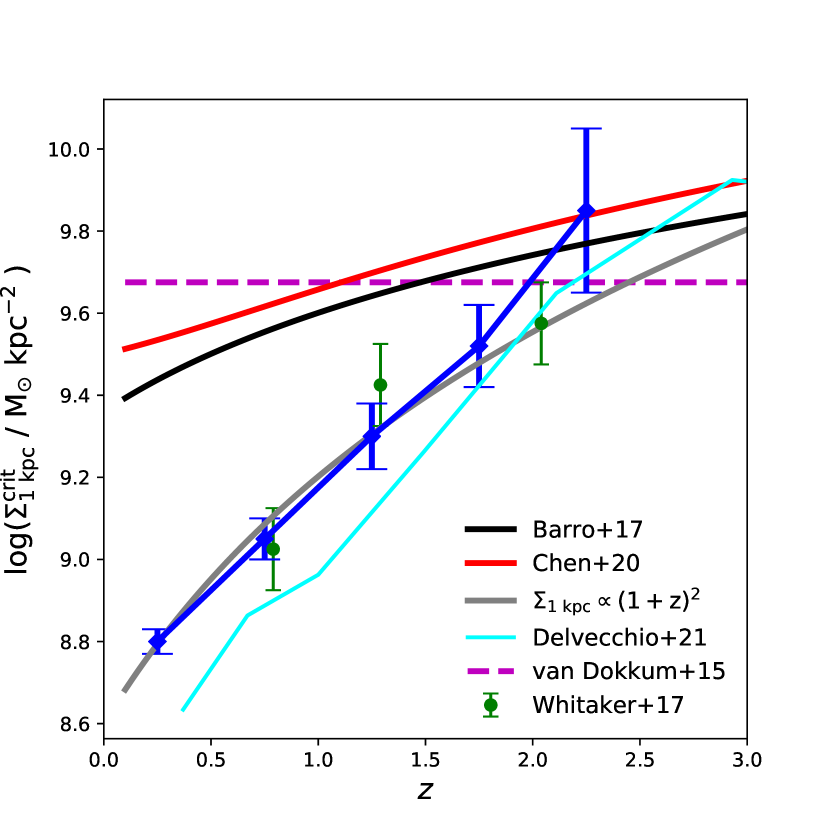
Figure 4: $\Sigma^{crit}_{1\ kpc}$ as a function of redshift (blue diamonds). Green circles are the critical $\Sigma_{1\ kpc}$ from Whitaker et al. (2017), assuming an evolving limit in log(sSFR). Gray dashed line indicates the expected cosmological evolution in surface density normalized at $z=0.25$, $\Sigma_{1\ kpc}\propto(1+z)^{2}$. Red solid line denotes the redshift dependence of the normalization of the quenching boundary from Chen et al. (2020), normalized at $z=2.25$. Black solid line marks the redshift evolution of the zero-point of scaling relation of QGs from Barro et al. (2017). Magenta dashed line is the assumed constant threshold in velocity dispersion above which galaxies quench at $1.5<z<3.0$ from van Dokkum et al. (2015). Cyan stars indicate the redshift evolution of $M_{0}$ which correponds the “bending” mass scale of the star-forming main sequence at each reshift. The data are from Delvecchio et al. (2021), and $M_{0}$ is converted to $\Sigma_{1\ kpc}$ using the scaling relations in Barro et al. (2017).

The significance of the redshift evolution in $\Sigma^{crit}_{1\ kpc}$ may rely on the definition of the transitional core density, which varies in different studies. In Barro et al. (2017); Chen et al. (2020), $\Sigma^{crit}_{1\ kpc}$ is defined as a boundary computed from the scaling relation of QGs, below which few quenched galaxies can be found. At the same time, as argued in Barro et al. (2017), such boundary is a necessary but not sufficient condition for quenching since there are some compact SFGs (cSFGs) found above the boundary. This boundary is essential to characterize the structural properties of the passive population, and its slow evolution (see black and red solid lines in Figure 4) likely reflects that a higher core density is a prerequisite to quenching and the core density is less affected by the minor mergers that contribute majority of the size growth in passive galaxies. Meanwhile, in (Whitaker et al., 2017; Xu & Peng, 2021) and this work, $\Sigma^{crit}_{1\ kpc}$ is computed based on a criteria of population-averaged color or sSFR. Though served in a statistical sense, the transitional core density defined in this way implicitly encodes the information of relative abundance of star-forming and passive populations in the sense that the abundance of QGs should be higher than that of SFGs above the boundary. Therefore, the strong evolution in $\Sigma^{crit}_{1\ kpc}$ (see blue diamonds in Figure 4) may attribute to the strong evolution in the number density of star-forming and passive populations (see Figure 1 and 10), combined with that $\Sigma_{1\ kpc}$ in QGs is typically higher than that of SFGs, at fixed stellar mass.

The weakly stellar mass-dependent $\Sigma^{crit}_{1\ kpc}$ implies that mass-quenching is more sensitive to the central core density than other global properties such as stellar mass. A natural candidate machanism is AGN feedback, since the BH mass is closely related to the central velocity dispersion and the central mass density (Fang et al., 2013; Bluck et al., 2014, 2020; Chen et al., 2020). As discussed in Xu & Peng (2021), the weakly mass-dependent $\Sigma^{crit}_{1\ kpc}$ is qualitatively consistent with the AGN feedback model prescription in IllustrisTNG (Terrazas et al., 2020), though the $M_{BH}^{crit}\sim 10^{8.2}M_{\odot}$ implemented in TNG is systematically higher than their inferred value in the local universe.

However, it is still challenging to account for the strong evolution in the population-averaged color or sSFR at fixed stellar mass and $\Sigma_{1\ kpc}$ (see Figure 2 and 11), or equivalently the strong evolution in $\Sigma^{crit}_{1\ kpc}$ at fixed stellar mass, if the core density or the central balck hole is the only quenching engine, since the quenching timescale due to AGN feedback is expected to be much shorter than $t_{Hubble}$. We attempt to interpret such strong evolution by the following scenarios. First, In the scenario of AGN feedback quenching, the integrated power output of AGN is dictated by the black hole mass, and the shutdown of star formation initiates as the integrated energy from the black hole becomes larger than the gravitational binding energy of gas within the halo (Terrazas et al., 2020; Chen et al., 2020; Piotrowska et al., 2022; Bluck et al., 2023). At a given stellar mass, the halo is on average more massive at higher redshift (Behroozi et al., 2019; Girelli et al., 2020), therefore the star formation swarmed with more gas requires a higher level of integrated energy from black hole or a more massive black hole to quench.

Second, the quenching process is also affected by the thermodynamical status of gas. As argued in (Dekel & Birnboim, 2006), at $z<2$ in massive halos with $M_{h}>M_{shock}$, the gas is inevitably heated by the virial shock, and it ultimately becomes diluted and more vulnerable to the feedback processes including AGN feedback. Hence a lower level of integrated energy (or a less massive black hole) may be required to quench the massive galaxies in halo with $M_{h}>M_{shock}$ in the hot accretion regimes at $z<2$. Meanwhile, the gas at $z>2$ is preferentially accreted in the form of cold stream instead of shock-heated medium. Hence, a more massive halo along with a more massive black hole are required to shock-heat the gas into “puffy” medium, thus enable the quenching due to AGN feedback to proceed in such cold accretion regimes. Therefore, the strong evolution in $\Sigma^{crit}_{1\ kpc}$ is likely to be a manifestation of the evolution of boundary between cold and hot medium, which is discussed in Dekel & Birnboim (2006).

There are some observational evidence to support the increasing mass scale with redshift, above which the cold gas supply is significantly reduced. For instance, some studies have argued that the “bending” of the star-forming main sequence (SFMS) at high mass end is likely due to the diminished cold gas supply by halo shock-heating (Delvecchio et al., 2021; Daddi et al., 2022; Popesso et al., 2023). Delvecchio et al. (2021) use a parametric form to quantitatively describe the “bending” of SFMS, and find that the characteristic “bending” mass $M_{0}$ has strong redshift evolution. We use the best-fitted $M_{\star}-\Sigma_{1\ kpc}$ scaling relations for SFGs to convert $M_{0}$ to $\Sigma_{1\ kpc}$ and plot them in Figure 4 (cyan stars). Interestingly, the slope of redshift evolution of $M_{0}$ matches that of $\Sigma^{crit}_{1\ kpc}$ very well, which lends support to the halo-heating scenario. However, such consistency remains only in a qualitative level, since halo-heating scenario predicts that the quenching should also strongly correlate with the halo or stellar mass, which is contradicting with the observed weakly mass-denpendent $\Sigma^{crit}_{1\ kpc}$. Moreover, galaxies that live in haloes with $M_{h}<M_{shock}$ are expected to be in cold accretion phase even at low redshifts, and quenching occurs in these galaxies cannot be interpreted by halo-heating solely. Therefore, it is likely that both AGN feedback and halo-heating are acting in concert to contribute the observed evolution in $\Sigma^{crit}_{1\ kpc}$.

Thirds, other alternative quenching mechanism may also become more effective at low redshifts, such as angular momentum quenching (Peng & Renzini, 2020; Renzini, 2020). As the disks grow with cosmic time, the average angular momentum of galaxies gradually increases. At low redshifts, the accreted gas spirals in with too high angular momentum to enable a fast radial gas inflow to feed the inner regions of galaxies. Instead, these infalling gas would settle onto an outer ring that is stable against fragmentation and radial migration. The star formation in the inner regions of galaxies would eventually be terminated due to the reduced gas supply or strangulation. As a consequence, a lower level of integrated energy from black hole is required as the quenching power.

Finally, we caution that the observed correlation between the quiescence and central mass density does not necessarily imply causality, and a higher $\Sigma_{1\ kpc}$ is likely to be the consequence of the quenching processes. At this stage, neither are we able to distangle the forementioned scenarios, nor to ascertain the causal direction, given the current data. Future cold gas survey (both HI and HII) and detailed comparison with the predictions from numerical simulations will be crucial to unveil the underlying physics of this structural evolution accompanying the quenching.

5 Acknowledgement

The authors wish to thank the anonymous referee for constructive comments that have improved the manuscript. This work is supported by the National Science Foundation of China (NSFC) Grant No. 12125301, 12192220, 12192222, and the science research grants from the China Manned Space Project with NO. CMS-CSST-2021-A07.

Appendix A Local Environmental Indicators for Galaxies at High Redshift

In this Appendix, we determine $N$ and $\delta z$ which are required to compute the local overdensity for the galaxies at high redshifts. We aim to select $N$ and $\delta z$ upon which the constructed local overdensity has the highest sensitivity to the the quiescence of galaxies. To achieve this, we study the quiescent fraction as a function of the rank of overdensity at three redshift bins: $0.5<z<1.0$, $1.0<z<1.5$ and $1.5<z<2.0$. In each redshift bin, we define 40 different local overdensities based on 8 choices of $N=3,4,5,6,7,8,9,10$ and 5 choices of $\delta z=0.04,0.06,0.08,0.1,0.12\times(1+z)$. The quiescent galaxies are selected via UVJ diagram and the quiescent fraction of galaxies is computed in an interval of 0.1 in the rank of overdensity for each definition, as shown in Figure 5.

We define an indicator which is the quiescent fraction in the densest bin (e.g. highest 10%), to quantitatively evaluate the sensitivity of quiescence to the local overdensity. We list the quiescent fraction in the densest bin as a function of $\delta z$ with multiple choices of $N$ in Figure 6. The best choice of $N$ and $\delta z$ appears to depend on the redshift, and there is no single choice of $N$ and $\delta z$ that prevails at all redshifts. For instance, at $0.5<z<1.0$, the quiescent fraction in densest bin is most sensitive to the overdensity with large $N$ ($N=10$) and small $\delta z$ ($\delta z$ = 0.04$\times(1+z)$), while small $N$ ($N=4$) and large $\delta z$ ($\delta z$ = 0.12$\times(1+z)$) appears a better choice at $1.0<z<1.5$. We then add up the quiescent fraction over all the three redshit bins for each $N$ and $\delta z$, and rank their performance. We find that the overdensity based on $N=8$ and $\delta z=0.08$ stands out to have the highest total quiescent fraction. Therefore, we use $N=8$ and $\delta z=0.08$ to compute the local overdensity of the galaxies at $0.5<z<2.5$ in this study.

Figure 5: Quiescent fraction as a function of local overdensity at three redshift bins. Different row denotes different choice of $\delta z$ in computing the overdensity. Eight choices of $N$ were used in each panel to compute the overdensity, as indicated by their colors.

Figure 6: Quiescent fraction in the densest bin as a function of $\delta z$ at three redshift bins. Eight choices of $N$ were used to compute the Quiescent fraction in the densest bin, as indicated by their colors.

Appendix B The correction of Dust Extinction

We evaluate the suitable $R_{V}$ used in the dust extinction law to correct the (U - V) color for the effect of dust extinction in this Appedix. We first utilize the UVJ diagram the select SFGs and QGs at $0.5<z<2.5$. We follow the same selection criteria used in Kawinwanichakij et al. (2017), in which the rest-frame color satisfies:

$$(U-V)_{0} >1.2\times(V-J)_{0}+0.2$$ (B1)

$$(U-V)_{0} >1.3$$

$$(V-J)_{0} <1.6.$$

We then test 7 choices of $R_{V}=2.1,2.6,3.1,3.6,4.1,4.6,5.1$. For each galaxy with a given value of $A_{V}$, we compute 7 corrected (U - V) color by assuming a Calzetti law and a choice of $R_{V}$. We find that the corrected color shows clear bimodality at almost all redshifts, and the color criteria that seperates the SFGs and QGs is always $\sim 1.2$ regardless of choice of $R_{V}$. Therefore, for each $R_{V}$, we use (U - V)${}_{cor}\sim 1.2$ as color criteria to classify SFGs and QGs. Each classification was compared with the one based on UVJ diagram and our aim is to select the classification with a suitable $R_{V}$ that best mimics the UVJ classification. We define the false positive rates for SFGs and QGs, respectively, to quantify the “similarity” of two classification schemes: $f_{FP}$ for SFGs is defined as the ratio of number of SFGs^UVJ with (U - V)${}_{cor}>1.2$ to the number of SFGs^UVJ, while $f_{FP}$ for QGs is defined as the ratio of number of QGs^UVJ with (U - V)${}_{cor}<1.2$ to the number of QGs^UVJ. We plot $f_{FP}$ as a function of redshift in Figure 7 for SFGs and QGs, respectively.

Figure 7: False positive rate for SFGs (QGs) as a function of redshift in left (right) panel. Seven $R_{V}$ were used in computing the false positive rate, as indicated by their colors.

As Shown in Figure 7, $f_{FP}$ for SFGs (QGs) generally decreases (increases) with the redshift. A higher $R_{V}$ tends to produce more(less) mis-classified SFGs(QGs). $f_{FP}$ for SFGs only has a mild redshift evolution, as $f_{FP}$ for SFGs is low on average (the highest $f_{F}P$ is $<0.1$), and variation in $f_{FP}$ over different $R_{V}$ is also small ($<0.05$); while $R_{V}$ has an stronger impact on the evolution of $f_{FP}$ for QGs, in particular at high redshifts. For instance, at $2.5<z<3.0$, $R_{V}=2.1$ will result in $f_{FP}>0.6$, which is much higher than $f_{FP}\sim 0.15$ with $R_{V}=5.1$. We plot (U - V)_cor as a function of stellar mass in four redshift bins with three different $R_{V}$ in Figure 8. As shown, a QGs is more likely to be mis-classified as a SFGs when using (U - V)_cor with a lower $R_{V}$, in particular at high redshift. Therefore, we adopt a relatively high value of $R_{V}=5.1$ in this study to correct the (U - V) color for galaxies at high redshifts.

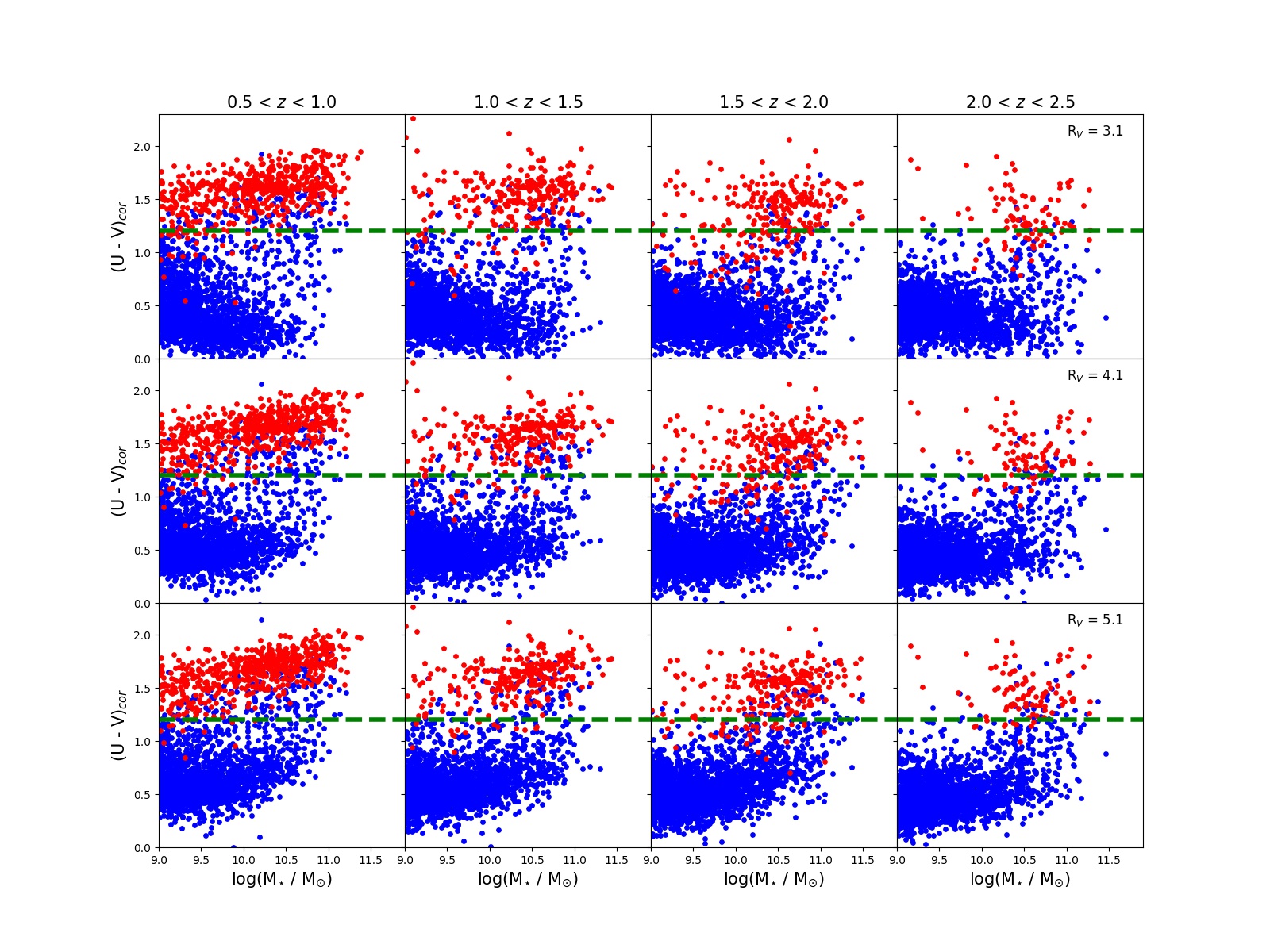
Figure 8: Dust-corrected rest-frame (U - V) color as a function of stellar mass at three redshift bins. Different row denotes different choice of $R_{V}$. Blue (red) data points are SFGs (QGs) identified by UVJ diagram. Green dashed lines marks the color criteria that seperates the star-forming and quenching in-process populations.

Appendix C Further explorations on stellar mass versus core density

C.1 $M_{\star}$ versus $\Sigma_{1\ kpc}$, color-coded by original (U - V)_cor

In Figure 1, we shift the color distribution of SDSS galaxies towards the left by 0.3 dex, and use the shifted color to evaluate the critical $\Sigma_{1\ kpc}$ for SDSS galaxies in Figure 2. We emphasize that such shifting has no impact on the determination of $\Sigma^{crit}_{1\ kpc}$, but to narrow down the color range across all the redshifts, and enhance the color contrast between the star-forming and quiescent populations for galaxies at high redshift. To avoid any confusion on this shifting, we plot $\Sigma_{1\ kpc}$ as a function of stellar mass, color-coded by their original color in Figure 9. We repeat the same precedures as in Section 3 to compute $\Sigma^{crit}_{1\ kpc}$, and found that they indeed remain the same as in Figure 2.

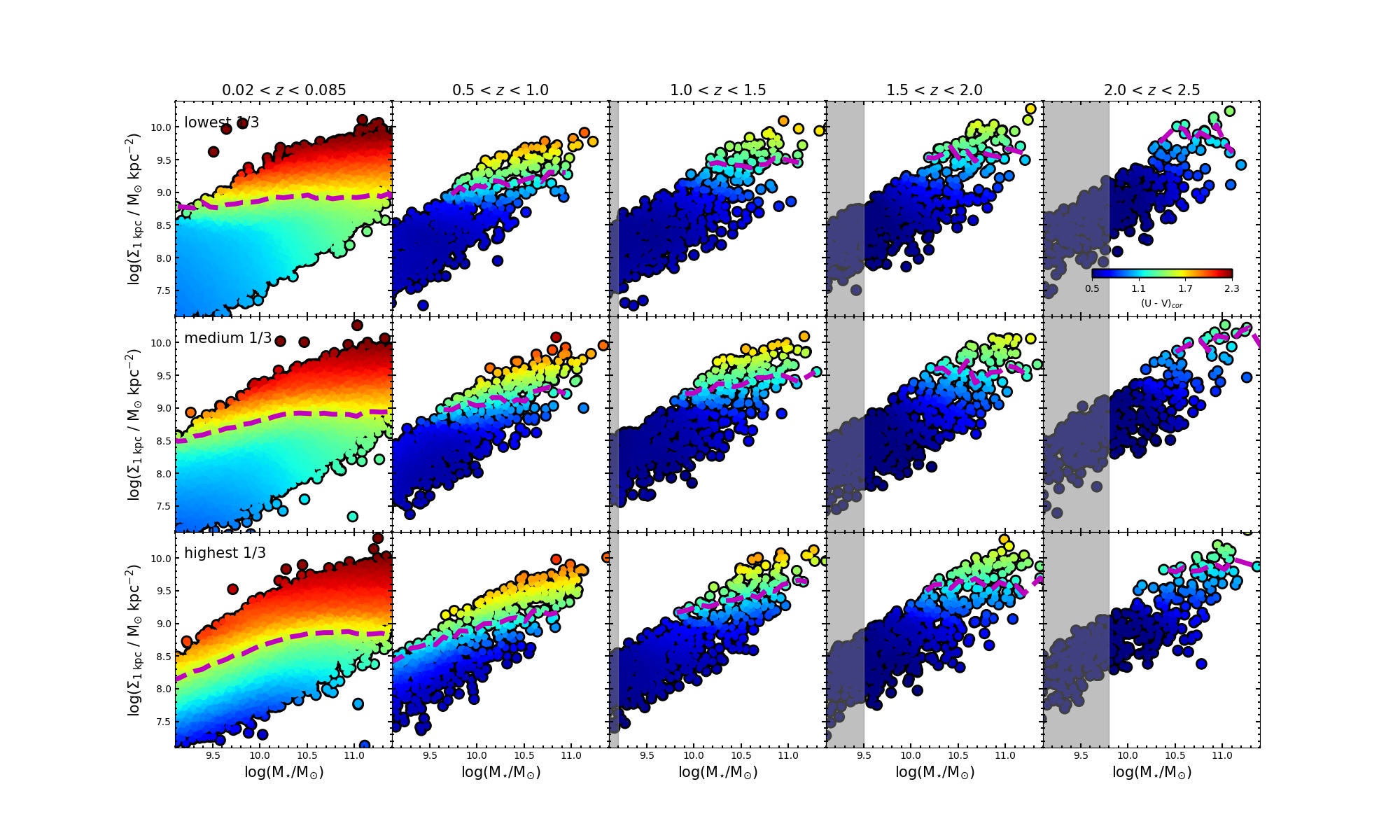
Figure 9: Similar to Figure 2. SDSS galaxies in the first column are color-coded by their original (U - V)_cor without shifting. The magenta dashed lines denote the transitional $\Sigma_{1\ kpc}$ at (U - V)_cor $\sim$ 1.55, as marked by the black dashed line in Figure 1.

C.2 $M_{\star}$ versus $\Sigma_{1\ kpc}$, color-coded by sSFR

In this Appendix, we explore the distribution of sSFR on the plane of $\rm M_{\star}-\Sigma_{1\ kpc}$. For SDSS galaxies, we utilize the data from the X2 version of Galaxy Evolution Explorer (GALEX)-SDSS-Wide-field Infrared Survey Explorer (WISE) Legacy Catalogue (GSWLC-X2, Salim et al., 2016, 2018), which is a value-added catalogue for SDSS galaxies at $0.01<z<0.3$ within GALEX All-sky Imaging survey footprint (Martin et al., 2005). SFRs are derived from SED fitting consisting of two GALEX UV bands, five SDSS optical and near-IR bands, and one mid infrared band (22 microns if available, otherwise 12 microns) from WISE (Wright et al., 2010). For ZFOURGE galaxies, SFRs are estimated by combining the total infrared luminosity ($L_{IR}$ = $L_{8-1000\mu m}$) of galaxies and the luminosity emitted in the UV ($L_{UV}$ at rest-frame 2800 $\AA$). The extracted 24 – 160 $\mu$m photometries from Spitzer/IRAC and MIPS images (in all fields) and Herschel/PACS images (available for CDFS only) were used to fit a model spectral template to calculate the total IR luminosity. $L_{UV}+L_{IR}$ provides an estimate of the total bolometric luminosity, which can be converted to SFR by (Bell et al., 2005):

$$SFR\,[M_{\odot}\,yr^{-1}]=1.09\times 10^{-10}\,(L_{IR}+2.2L_{UV})$$ (C1)

We refer the readers to Section 6 in Straatman et al. (2016) for more details.

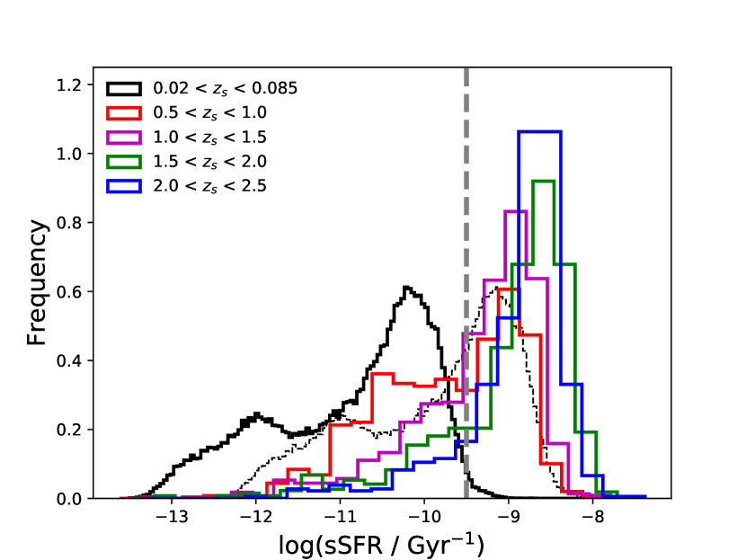
Figure 10: Distribution of specific SFR at five redshift bins. We shift the original disribution of sSFR for SDSS galaxies (black solid line) to the right by 1 dex (thin dashed line), to ease comparison of color distribution on the $\rm M_{\star}-\Sigma_{1\ kpc}$ plane. Gray dahsed line marks the critical sSFR that roughly separates the star-forming and quiescent populations at all redshifts, which is $\rm log(sSFR/Gyr^{-1})\sim-9.5$.

We plot the distribution of sSFR for galaxies with $\rm log(M_{\star}/M_{\odot})>9.8$ at five redshift bins in Figure 10. In general, sSFR also exhibits strong redshift evolution and galaxies have higher sSFR at higher redshifts. Similar to the case of (U - V) color, a critical sSFR that separates the star-forming and passive populations is vital for the computation of $\Sigma^{crit}_{1\ kpc}$. As shown in Figure 10, the star-forming population with $\rm log(sSFR/Gyr^{-1})>-9.5$ dominates at $z>1$, and a noticable bump with $\rm log(sSFR/Gyr^{-1})<-9.5$ emerges at $0.5<z<1$, which represents the increasing passive population. sSFR at $z\sim 0$ (SDSS galaxies) is much lower than their high redshift counterparts, and shows clear bimodality. Following the same logic to ease comparison as in Figure 1, we shift the distribution of sSFR by 1 dex towards the right in Figure 10 (thin dashed line). We refrain from sophisticatelly modeling the evolving criteria in sSFR as a function of redshift, since we only attempt to inspect if the trend in $\Sigma^{crit}_{1\ kpc}$ based on sSFR is consistent with that on (U - V)_cor. Instead, we adopt a simple criteria $\rm log(sSFR/Gyr^{-1})\sim-9.5$ that roughly separates the two populations at all redshifts. Moreover, since the passive population in this study not only consists of fully quenched galaxies, but also galaxies that are in the process of being quenched (e.g. Green Valley galaxies), the adopted critical sSFR is slightly higher than the commonly quoted criteria in literatures.

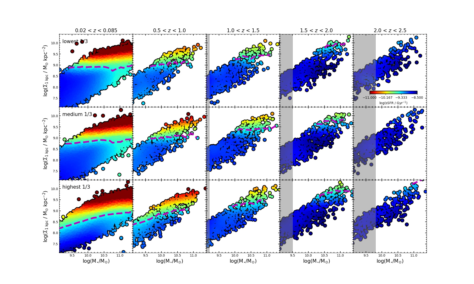
Figure 11: Similar to Figure 2. Galaxies are color-coded by their sSFR. The magenta dashed lines denote the transitional $\Sigma_{1\ kpc}$ at $\rm log(sSFR/Gyr^{-1})\sim-9.5$.

We follow the similar procedures described in Section 3 to assign galaxies into several redshift and environment bins, and plot $\Sigma_{1\ kpc}$ as a function of stellar mass, color-coded by their sSFR in Figure 11. $\Sigma^{crit}_{1\ kpc}$ is computed as the running median of $\Sigma_{1\ kpc}$ that have $\rm-9.5-0.15<log(sSFR/Gyr^{-1})<-9.5+0.15$. We overplot $\Sigma^{crit}_{1\ kpc}$ as the magenta dashed lines in Figure 11. As shown, the trends in $\Sigma^{crit}_{1\ kpc}$ are very similar with those base upon (U - V)_cor.

Appendix D Stellar mass versus overdensity

In this Appendix, we investigate the relationship between the core density and the overdensity at $0<z<2.5$, to gain complete insight of the effects of environment. We assign galaxies into five redshift bins to study their redshift evolution. We divide the galaxies in each redshift bin into six stellar mass bins to study their stellar mass dependence. We perform a $V_{max}$-weighting correction for each SDSS galaxy to correct for the incompleteness, inside a box of $0.2\times 0.2$ dex² that centers on each data point. The data in each bin has been LOESS smoothed. $\Sigma^{crit}_{1\ kpc}$ is computed based on the color criteria of (U - V)_cor $\sim$ 1.25. We plot $\Sigma_{1\ kpc}$ as a function of the rank of log(1 + $\delta$), color-coded by their (U - V)_cor in Figure 12. $\Sigma^{crit}_{1\ kpc}$ are overplotted as the magenta dashed lines for reference.

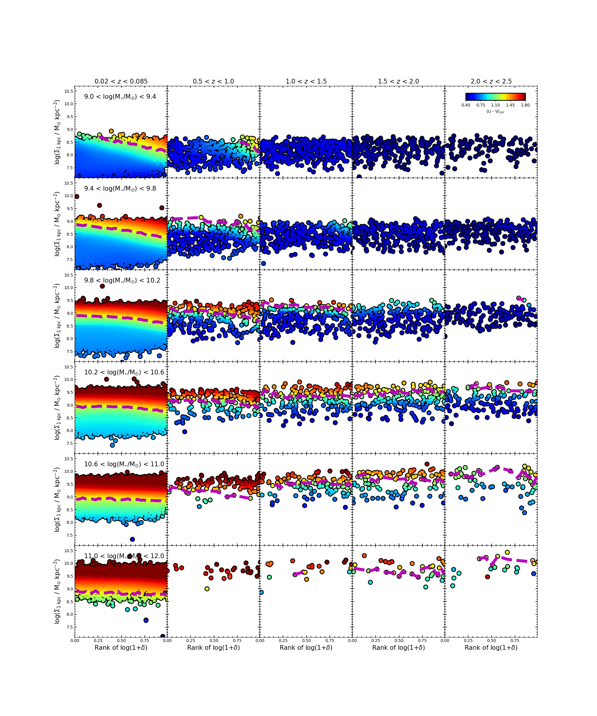
Figure 12: Central 1kpc surface mass density $\Sigma_{1\ kpc}$ as a function of the rank of overdensity log(1+$\delta$) at five redshift bins (different columns) and six stellar mass bins (different rows), color-coded by the dust-corrected (U - V) color. the data at $0.02<z<0.085$ (SDSS galaxies) has been $V_{max}$-weighted. The data in each bin has been LOESS smoothed. The magenta dahsed lines denote the transitional $\Sigma_{1\ kpc}$ at (U - V)_cor $\sim$ 1.25.

For massive galaxies with $log(M_{\star}/M_{\odot})>10.2$, the color is very strongly correlated with $\Sigma_{1\ kpc}$ and independent on the environment, as indicated by the almost flat $\Sigma^{crit}_{1\ kpc}$. $\Sigma^{crit}_{1\ kpc}$ in all environments exhibits similar strong redshift evolution as depicted in the left panel of Figure 3. This is likely due to that large portion of massive galaxies are mass-quenched at high redshift, when the enviromental effects have yet to come into play. Quenching in these galaxies might occur in advance of their infall into dense environments.

For galaxies with intermediate and low mass, the environmental impact becomes progressively significant at $z<1$, as dictated by the gradual tilt in $\Sigma^{crit}_{1\ kpc}$. At fixed stellar mass, $\Sigma^{crit}_{1\ kpc}$ appears inversely proportional to the overdensity. For instance, in the lowest mass bin of $9.0<log(M_{\star}/M_{\odot})<9.4$ at $0.02<z<0.085$, $\Sigma^{crit}_{1\ kpc}$ in densest environment is $\sim 0.7$ dex lower than that in sparse environment. Such inversely proportionality was first reported in Xu & Peng (2021) for nearby galaxies, and our study shows that it has already been in place at $z\sim 1$ (see second column in Figure 12). It could be qualitatively accounted for by two facts, as suggested in Xu & Peng (2021): 1. there are more quenched galaxies in dense environments at fixed stellar mass; 2. the color of galaxies is strongly correlated with their structure such as $\Sigma_{1\ kpc}$. Intriguingly, the environmental effects such as gas stripping is not supposed to significantly alter the stellar structure of galaxies. An almost vertical $\Sigma^{crit}_{1\ kpc}$ is anticipated if gas stripping is the dominant effect of environment. Therefore, a tilted but non-vertical $\Sigma^{crit}_{1\ kpc}$ would cast valuable contraints on the underlying physical mechanisms of environmental quenching. After all, a strong correlation between the color and $\Sigma_{1\ kpc}$ at fixed stellar mass favors those scenarios in which the structure of galaxies could be altered by the environmental effects, such as tidal interaction or minor merger.

We also plot $\Sigma_{1\ kpc}$ as a function of rank of log(1 + $\delta$), color-coded by their sSFR in Figure 13 for reference. $\Sigma^{crit}_{1\ kpc}$ is computed based on $\rm log(sSFR/Gyr^{-1})\sim-9.5$, as the magenta dashed lines denote. The trends in $\Sigma^{crit}_{1\ kpc}$ remains similar as those in Figure 12.

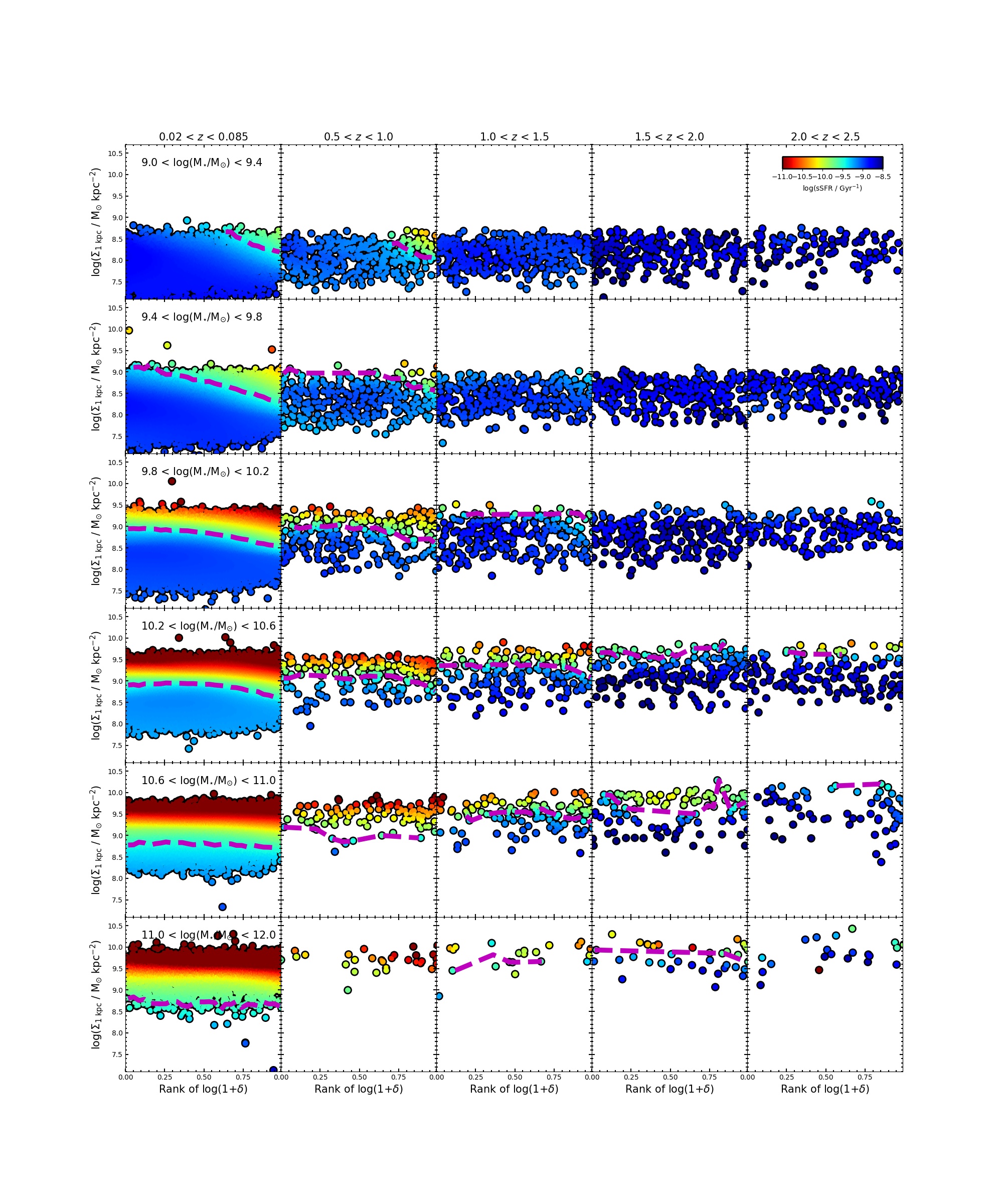
Figure 13: Similar to Figure 12. Galaxies are color-coded by their sSFR. The magenta dashed lines denote the transitional $\Sigma_{1\ kpc}$ at $\rm log(sSFR/Gyr^{-1})\sim-9.5$.

References

- Abadi et al. (1999) Abadi, M. G., Moore, B., & Bower, R. G. 1999, MNRAS, 308, 947
- Abazajian et al. (2009) Abazajian, K. N., Adelman-McCarthy, J. K., Agüeros, M. A., et al. 2009, ApJS, 182, 543
- Baldry et al. (2006) Baldry, I. K., Balogh, M. L., Bower, R. G., et al. 2006, MNRAS, 373, 469
- Balogh et al. (1997) Balogh, M. L., Morris, S. L., Yee, H. K. C., Carlberg, R. G., & Ellingson, E. 1997, ApJL, 488, L75
- Barro et al. (2017) Barro, G., Faber, S. M., Koo, D. C., et al. 2017, ApJ, 840, 47
- Behroozi et al. (2019) Behroozi, P., Wechsler, R. H., Hearin, A. P., et al. 2019, MNRAS, 488, 3143
- Bell et al. (2005) Bell, E. F., Papovich, C., Wolf, C., et al. 2005, ApJ, 625, 23
- Bell et al. (2012) Bell, E. F., van der Wel, A., Papovich, C., et al. 2012, ApJ, 753, 167
- Bezanson et al. (2009) Bezanson, R., van Dokkum, P. G., Tal, T., et al. 2009, ApJ, 697, 1290
- Blanton & Roweis (2007) Blanton, M. R., & Roweis, S. 2007, AJ, 133, 734
- Bluck et al. (2014) Bluck, A. F., Mendel, J. T., Ellison, S. L., et al. 2014, MNRAS, 441, 599
- Bluck et al. (2020) Bluck, A. F. L., Maiolino, R., Piotrowska, J. M., et al. 2020, MNRAS, 499, 230
- Bluck et al. (2023) Bluck, A., Piotrowska, J. M., Maiolino, R. 2023, ApJ, 944, 108
- Brammer et al. (2008) Brammer, G. B., van Dokkum, P. G., & Coppi, P. 2008, ApJ, 686, 1503
- Cappellari et al. (2006) Cappellari, M., Bacon, R., Bureau, M., et al. 2006, MNRAS, 366, 1126
- Cappellari et al. (2013) Cappellari, M., et al., 2013, MNRAS,432, 1862
- Cappellari et al. (2006) Cappellari, M., Bacon, R., Bureau, M., et al. 2006, MNRAS, 366, 1126
- Chen et al. (2020) Chen, Z., Faber, S. M., Koo, D. C., et al. 2020, ApJ, 897, 102
- Cheung et al. (2012) Cheung, E., Faber, S. M., Koo, D. C., et al. 2012, ApJ, 760, 131
- Ciotti & Bertin (1999) Ciotti, L., & Bertin, G. 1999, A& A, 352, 447
- Cleveland & Devlin (1988) Cleveland, W. S., & Devlin, S. J., 1988, J. AM. Stat. Assoc, 83, 596
- Croton et al. (2006) Croton, D. J., Springel, V., White, S. D. M., et al. 2006, MNRAS, 365, 11
- Daddi et al. (2022) Daddi, E., Delvecchio, I., Dimauro, P., et al. 2022, A&A, 661, L7
- Darvish et al. (2015) Darvish, B., Mobasher, B., Sobral, D., Scoville, N., & Aragon-Calvo, M.2015, ApJ, 805, 121
- Darvish et al. (2016) Darvish, B., Mobasher, B., Sobral, D., et al. 2016, ApJ, 825,113
- De Lucia et al. (2019) De Lucia, G., Hirschmann, M., & Fontanot, F. 2019, MNRAS, 482, 5041
- Delvecchio et al. (2021) Delvecchio, I., Daddi, E., Sargent, M. T., et al. 2021, A&A, 647, A123
- Dekel & Birnboim (2006) Dekel, A. & Birnboim, Y. 2006, MNRAS, 368, 2
- Draine et al. (2003) Draine, B. T. 2003, ARA&A, 41, 241
- Fitzpatrick (1999) Fitzpatrick, E. L. 1999, PASP, 111, 63
- Fang et al. (2013) Fang, J. J., Faber, S. M., Koo, D. C., & Dekel, A. 2013, ApJ, 776, 63
- Genzel et al. (2014) Genzel, R., Förster Schreiber, N. M., Lang, P., et al. 2014, ApJ, 785, 75
- Giacconi et al. (2002) Giacconi, R., Zirm, A., Wang, J., et al. 2002, ApJS, 139, 369
- Girelli et al. (2020) Girelli, G., Pozzetti, L., Bolzonella, M., et al. 2020, A&A, 634, A135
- Grogin et al. (2011) Grogin, N. A., Kocevski, D. D., Faber, S. M., et al. 2011, ApJS, 197, 35
- Gunn & Gott (1972) Gunn, J. E., & Gott, J. R., III 1972, ApJ, 176, 1
- Guo et al. (2021) Guo, Y., Carleton, T., Bell, E., et al. 2021, ApJ, 914, 7
- Kauffmann & Heckman (2003) Kauffmann, G., & Heckman, T. M. 2003, MNRAS, 1077, 1055
- Kawinwanichakij et al. (2017) Kawinwanichakij, L., Papovich, C., Quadri, R. F., et al. 2017, ApJ, 847, 134
- Kennedy et al. (2015) Kennedy, R., Bamford, S., Baldry, I., et al. 2015, MNRAS, 454, 806
- Kodra et al. (2023) Kodra, D., Andrews, B. H., Newman, J. A., et al. 2023, ApJ, 942, 36
- Koekemoer et al. (2011) Koekemoer, A. M., Faber, S. M., Ferguson, H. C., et al. 2011, ApJS, 197, 36
- Lawrence et al. (2007) Lawrence, A., Warren, S. J., Almaini, O., et al. 2007, MNRAS, 379, 1599
- Lin et al. (2016) Lin, L., Capak, P. L., Laigle, C., et al. 2016, ApJ, 817, 97
- Luo et al. (2020) Luo, Y., Faber, S. M., Rodríguez-Puebla, A., et al. 2020, MNRAS, 493, 168
- Martig et al. (2009) Martig, M., Bournaud, F., Teyssier, R. et al. 2009, ApJ, 707, 250
- Martin et al. (2005) Martin D. C., et al., 2005, ApJ, 619, L1
- Mathis et al. (1990) Mathis, J. S. 1990, ARA&A, 28, 376
- Muldrew et al. (2012) Muldrew, S. I., Croton, D. J., Skibba, R. A., et al. 2012, MNRAS, 419, 2670
- Peng et al. (2010) Peng, Y., Lilly, S. J., Kovac, K., et al. 2010, ApJ, 721, 193
- Peng et al. (2012) Peng, Y., Lilly, S. J., Renzini, A., & Carollo, M., 2012, ApJ, 757, 4
- Peng & Renzini (2020) Peng, Y. J., & Renzini, A. 2020, MNRAS, 491, L51
- Piotrowska et al. (2022) Piotrowska, J. M., Bluck, A., Maiolino, R., et al. 2022, MNRAS, 512, 1052
- Popesso et al. (2023) Popesso, P., Concas, A., Cresci, G., et al. 2023, MNRAS, 519, 1526
- Renzini (2020) Renzini, A. 2020, MNRAS, 495, L42
- Salim et al. (2007) Salim, S., Rich, R. M., Charlot, S., et al. 2007, ApJS, 173, 267
- Salim et al. (2016) Salim S., et al., 2016, ApJS, 227, 2
- Salim et al. (2018) Salim S., Boquien M., Lee J. C., 2018, ApJ, 859, 11
- Scoville et al. (2007) Scoville, N., Aussel, H., Brusa, M., et al. 2007, ApJS, 172, 1
- Simard et al. (2011) Simard L., Mendel J. T., Patton D. R., Ellison S. L., McConnachie A. W., 2011, ApJS, 196, 11
- Skelton et al. (2014) Skelton, R., Whitaker, K. E., Momcheva, I. G., et al. 2014, ApJS, 214, 24
- Sobral et al. (2011) Sobral, D., Best, P. N., Smail, I., et al. 2011, MNRAS, 411, 675
- Straatman et al. (2016) Straatman, C. M., Spitler, L., Quadri, R., et al. 2016, ApJ, 830, 51
- Tacchella et al. (2015) Tacchella, S., Carollo, C. M., Renzini, A., et al. 2015, Sci, 348, 314
- Terrazas et al. (2020) Terrazas B. A., et al., 2020, MNRAS, 493, 1888
- van der Wel et al. (2012) van der Wel, A., Bell, E. F., Haussler, B., et al. 2012, ApJS, 203, 24
- van Dokkum et al. (2014) van Dokkum, P. G., Bezanson, R., van der Wel, A., et al. 2014, ApJ, 791, 45
- van Dokkum et al. (2015) van Dokkum, P. G., Nelson, E. J., Franx, M., et al. 2015, ApJ, 813, 23
- Whitaker et al. (2017) Whitaker, K. E., Bezanson, R., van Dokkum, P. G., et al. 2017, ApJ, 838, 19
- Williams et al. (2010) Williams, R. J., Quadri, R. F., Franx, M., et al. 2010, ApJ, 713, 738
- Woo et al. (2017) Woo, J., Carollo, C. M., Faber, S. M., Dekel, A., & Tacchella,S. 2017,MNRAS, 464, 1077
- Wright et al. (2010) Wright E. L., et al., 2010, AJ, 140, 1868
- Xu & Peng (2021) Xu, B., & Peng, Y. 2021, ApJ, 923, L29
- Zinger et al. (2020) Zinger, E., et al., 2020, MNRAS, 499, 768