Analyzing the Impact of Tax Credits on Households in Simulated Economic Systems with Learning Agents

Abstract

In economic modeling, there has been an increasing investigation into multi-agent simulators. Nevertheless, state-of-the-art studies establish the model based on reinforcement learning (RL) exclusively for specific agent categories, e.g., households, firms, or the government. It lacks concerns over the resulting adaptation of other pivotal agents, thereby disregarding the complex interactions within a real-world economic system. Furthermore, we pay attention to the vital role of the government policy in distributing tax credits. Instead of uniform distribution considered in state-of-the-art, it requires a well-designed strategy to reduce disparities among households and improve social welfare. To address these limitations, we propose an expansive multi-agent economic model comprising reinforcement learning agents of numerous types. Additionally, our research comprehensively explores the impact of tax credit allocation on household behavior and captures the spectrum of spending patterns that can be observed across diverse households. Further, we propose an innovative government policy to distribute tax credits, strategically leveraging insights from tax credit spending patterns. Simulation results illustrate the efficacy of the proposed government strategy in ameliorating inequalities across households.

1 Introduction

In the domain of economic modeling, the spotlight has shifted towards multi-agent simulators. Recent papers like (Buşoniu, Babuška, and De Schutter 2010; Nowé, Vrancx, and De Hauwere 2012; Zheng et al. 2022; Curry et al. 2022) have contributed insights into the dynamics among households, firms, and the government. Furthermore, a line of literature, e.g., (Dosi and Roventini 2019; Axtell and Farmer 2022; Haldane and Turrell 2019; Liu et al. 2022; Hill, Bardoscia, and Turrell 2021; Chen et al. 2021), illuminates the impressive results of reinforcement learning (RL) within economic modeling. A pivotal contribution by (Sinitskaya and Tesfatsion 2015) proposes an economic model characterized by uniform consumer-workers and firms responsible for price and wage setting. Moreover, the work (Curry et al. 2022) introduces a more complicated model including consumers, firms, and the government, and learns an equilibrium in open real-business-cycle models.

Nonetheless, the research mentioned above does possess certain limitations that need to be addressed. Firstly, the papers (Dosi and Roventini 2019; Axtell and Farmer 2022; Haldane and Turrell 2019; Liu et al. 2022; Sinitskaya and Tesfatsion 2015; Hill, Bardoscia, and Turrell 2021) confine the utilization of reinforcement learning to a select category of agents, thereby lacking the modeling of other adaptive agents (such as the government or the central bank or both). This issue inadvertently neglects the complexities of real-world economic systems. Secondly, state-of-the-art such as (Curry et al. 2022) uniformly distribute tax credits and neglect the significance of government intervention in maintaining social welfare through tax collection and redistribution. Even though a recent paper (Liu et al. 2022) proposed an efficient algorithm to achieve social welfare maximization and competitive equilibrium simultaneously in the economic system, it only considers two types of agents, i.e., agents and planners.

To design an optimal tax credit distribution strategy, it’s important to study the tax credit spending patterns across various household types. In light of a comprehensive research report by JP Morgan Chase (Wheat, Deadman, and Sullivan 2022), household liquidity, defined as the ratio of savings to consumption, emerges as a powerful predictor of consumption behavior when tax credits are distributed to households. The report shows that low-liquidity households tend to allocate a larger proportion of their tax credits towards consumption, as opposed to higher-liquidity households. Notably, the spending patterns across various household types remain unexplored in multi-agent-based economic systems. Understanding these spending patterns is crucial for policymakers and economists aiming to formulate targeted and effective tax credit distribution policies. By studying the consumption behaviors of low-liquidity households, valuable insights can be gained into their financial challenges and needs. Such insights can inform the development of an effective credit distribution strategy, ultimately promoting welfare and economic growth.

Our paper models the dynamics and objectives of households, firms, central bank and the government in a multi-agent simulator. By enabling learning based strategies for each of the various agent types, we aim to create a more realistic and nuanced representation of the economic system. By integrating the central bank’s activities into our analysis, we capture the pivotal role it plays by adjusting interest rates to manage inflation and achieve GDP targets (Blinder et al. 2008). Moreover, we offer a comprehensive investigation of the impact of tax credit allocation on diverse household behavior. Based on this investigations, we design a government policy to facilitate an equitable distribution of tax credits to promote social welfare.

Our contributions are summarized as follows:

• We consider a multi-agent economic model that encompasses households, a firm, the central bank, and the government. Our implementation of this simulator builds upon a state-of-the-art simulator for financial markets (Byrd, Hybinette, and Balch 2019) and its extension (Amrouni et al. 2021).

• For an exploration of the spending behaviors of high-liquidity and low-liquidity households in response to tax credits, we introduce an innovative household dynamics model. This model incorporates a new action to capture distinct spending patterns. Simulation outcomes reveal that lower-liquidity households tend to spend a greater share of their tax credits, aligning with the findings observed in a JP Morgan Chase report (Wheat, Deadman, and Sullivan 2022).

• Leveraging the insights from the tax credit spending patterns, we propose a novel government strategy aimed at optimizing the distribution of tax credits to enhance overall social welfare. Our simulation results confirm the effectiveness of this proposed strategy, illustrating its potential to mitigate inequalities among diverse households.

2 Economic model

In this section, we present an economic model that involves households earning labor income from a firm and consuming goods, the firm producing goods using household labor, the government collecting income tax from households, and distributing tax credits to households (Krusell and Smith 1998; Evans and Honkapohja 2005; Benhabib, Schmitt-Grohé, and Uribe 2001). At the same time, the central bank sets the interest rate to achieve target inflation and improve the GDP (Kaplan, Moll, and Violante 2018; Svensson 2020). Distinguished from state-of-the-art, every agent in our system uses reinforcement learning to adapt their strategies to maximize individual objectives. Thus, providing a more comprehensive understanding of the dynamics of the economic model in the real world.

Our economic model with multiple reinforcement learning agents can be formalized as a Markov Game (MG) with each agent having partial observability of the global system state (Littman 1994; Hu, Wellman et al. 1998). The MG consists of finite-length episodes of $H$ time steps where each time step $t\in\{0,1,\cdots,H-1\}$ corresponds to one-quarter of economic simulation. We detail the model concerning each type of agent below. Agents’ parameters, observations, actions, and rewards are summarized in Table 1.

Agent	Observation	Action	Reward
Household $i$	$(m_{t,i},r_{t},\tau_{t},\kappa_{t,i},p_{t},w_{t}\par\par)$ $m_{t,i}$: saving $r_{t}$: interest rate $\tau_{t}$: tax rate $\kappa_{t,i}$: tax credit $p_{t}$: price of good set by firm $w_{t}$: wage set by firm	$(n_{t,i},c_{t,i}^{act})$ $n_{t,i}$: labor hours $c_{t,i}^{act}$: requested consumption	(2)
	Parameter
	$(\gamma_{i},\nu_{i},\mu_{i})$ $\gamma_{i}$: parameter for isoelastic utility of consumption and savings $\nu_{i}$: coefficient for disutility of labor $\mu_{i}$: coefficient for isoelastic utility of savings
Firm	$({\epsilon_{t-1}},Y_{t},{p_{t},}w_{t},\sum_{i}n_{t,i},\sum_{i}c_{t,i})$ $\epsilon_{t-1}$: exogenous production factor $\varepsilon_{t}$: production shock $Y_{t}$: inventory of firm $n_{t,i}$: labor hours of household $i$ $c_{t,i}$: realized consumption of household $i$	$(w_{t+1},p_{t+1})$	(4)
	Parameter
	$(\alpha,\rho,\sigma,\chi)$ $\alpha$: efficiency of production using labor $\rho$: auto-regression coefficient for production factor $\sigma$: standard deviation of production shock $\chi$: coefficient for inventory risk
Central Bank	$(p_{t-4},p_{t},y_{t})$ Calculates inflation $\pi_{t}$ using (5)	$r_{t+1}$	(6)
Government	$(\tau_{t},\{\kappa_{t,i}\}_{i},\sum_{i}\tau_{t}n_{t,i}w_{t})$	$(\tau_{t+1},\{\kappa_{t+1,i}\}_{i})$	(7)

Table 1: Summary of parameters, observations, actions, and rewards of agents in the economic model.

2.1 Households

At each time step $t$, household $i$ works for $n_{t,i}$ hours and attempts to consume $c^{act}_{t,i}$ units of the good produced by the firm. The good’s price is set by the firm as $p_{t}$, and an income tax rate is set by the government as $\tau_{t}$. Furthermore, the realized consumption of households depends on the available inventory of goods $Y_{t}$. The total demand for goods produced by the firm is given by $\sum_{i}c_{t,i}^{act}$. If there is insufficient supply to meet the demand, goods are rationed proportionally among households as follows:

$$c_{t,i}=\min\left\{c_{t,i}^{act},Y_{t}\cdot\frac{c_{t,i}^{act}}{\sum_{i}c_{t,i}^{act}}\right\}.$$

Household savings increase according to the interest rate $r_{t}$ set by the central bank. Additionally, consumption and work affect a household’s savings $m_{t}$. Household $i$ receives labor income equal to $n_{t,i}w_{t}$, where the firm pays a wage $w_{t}$.

The cost of consumption for household $i$ is given by $p_{t}\cdot c_{t,i}$. Moreover, with a flat tax rate of $\tau_{t}$, households pay income tax amounting to $\tau_{t}\cdot n_{t,i}w_{t}$. The government redistributes the tax revenue as tax credits $\kappa_{t,i}$ to ease household budgetary constraints. Considering all these factors, household savings change according to the following equation:

$$m_{t+1,i}= \left(1+r_{t}\right)m_{t,i}+\left(n_{t,i}w_{t}-p_{t}c_{t,i}\right)$$ (1)

$$-{\tau_{t}n_{t,i}w_{t}}+\kappa_{t,i}.$$

Each household $i$ optimizes its labor hours and consumption to maximize utility (Evans and Honkapohja 2005):

$$\max_{\left\{n_{t,i},c_{t,i}^{act}\right\}_{t=0}^{H-1}}\sum_{t=0}^{H-1}\beta_{i,\mathbf{H}}^{t}u\left(c_{t,i},n_{t,i},m_{t+1,i};\gamma_{i},\nu_{i},\mu_{i}\right)$$

where

$$u(c,n,m;\gamma,v,\mu)=\frac{c^{1-\gamma}}{1-\gamma}+\mu\operatorname{sign}(m)\frac{|m|^{1-\gamma}}{1-\gamma}-\nu n^{2}$$ (2)

with $\beta_{i,\mathbf{H}}$ being the household’s discount factor. The utility function is a sum of isoelastic utility from consumption with parameter $\gamma_{i}$, isoelastic utility from savings with parameter $\gamma_{i}$ and coefficient $\mu_{i}$, and a quadratic disutility of work with coefficient $\nu_{i}$.

2.2 Firm

At each time step, the firm employs households to produce goods and earns money from consumed goods. At time step $t$, it determines a price $p_{t+1}$ for its goods and selects a wage $w_{t+1}$ to pay, which will come into effect at the next time step $t+1$.

Based on the total labor hours $\sum_{i}n_{t,i}$, the firm produces $y_{t}$ units of goods per the following Cobb-Douglas production function (Cobb and Douglas 1928):

$$y_{t}=\epsilon_{t}\left(\sum_{i}n_{t,i}\right)^{\alpha}$$ (3)

where $0\leq\alpha\leq 1$ characterizes the efficiency of production using labor. And, $\epsilon_{t}$ is the exogenous production factor which follows a log-autoregressive process with coefficient $0\leq\rho\leq 1$ given by

$$\epsilon_{t}=\left(\epsilon_{t-1}\right)^{\rho}\exp\left(\varepsilon_{t}\right),$$

which allows for an exponential increase with a shock $\varepsilon_{t}\sim\mathcal{N}(0,\sigma^{2})$.

Furthermore, households purchase $\sum_{i}c_{t,i}$ units of the goods produced by the firm. Consequently, the inventory of the firm changes as $Y_{t+1}=Y_{t}+y_{t}-\sum_{i}c_{t,i}$. The firm optimizes the prices of its goods and the wages of households to maximize profits, resulting in the following formulation:

$$\max_{\{w_{t},p_{t}\}_{t=0}^{H-1}}\sum_{t=0}^{H-1}\beta_{\mathbf{F}}^{t}\left(p_{t}\sum_{i}c_{t,i}-w_{t}\sum_{i}n_{t,i}-\chi p_{t}Y_{t+1}\right),$$ (4)

where $\beta_{\mathbf{F}}$ represents the firm’s discount factor, $\chi>0$ is the regularization coefficient to restrict the firm from overly increasing the price to make profits without a subsequent increase in consumption. One can interpret this term as the risk of holding inventory as a result of producing much more than the expected consumption in the absence of the assumption of market clearing.

2.3 Central Bank

The central bank gathers data on annual price changes and the production of the firm at each time step. At time step $t$, the central bank sets the interest rate $r_{t+1}$, which will come into effect in the economic system at the next time step $t+1$. The annual inflation rate at time step $t$ is derived by the central bank based on the annual price changes and is calculated as:

$$\pi_{t}=\frac{p_{t}}{p_{t-4}}.$$ (5)

Additionally, the central bank evaluates the GDP using the production of the firm $y_{t}$. The central bank optimizes its monetary policy strategy to achieve its inflation and GDP targets as follows (Svensson 2020; Hinterlang and Tänzer 2021):

$$\max_{\left\{r_{t}\right\}_{t=0}^{H-1}}\sum_{t=0}^{H-1}\beta_{\bf{CB}}^{t}\left(-\left(\pi_{t}-\pi^{\star}\right)^{2}+\lambda y_{t}^{2}\right),$$ (6)

where $\beta_{\mathbf{CB}}$ represents the central bank’s discount factor, $\lambda>0$ is the weight given to productivity relative to the inflation target, and $\pi^{\star}$ is the desired inflation target.

2.4 Government

At time step $t$, the government collects income taxes denoted by $\sum_{i}\tau_{t}n_{t,i}w_{t}$, and sets the tax rate $\tau_{t+1}$ that will be effective at the next time step $t+1$. At time step $t$, the government distributes the collected tax revenue through tax credits $\kappa_{t+1,i}$ that will be distributed to household $i$ at the next time step $t+1$.

The government optimizes its choice of tax rate and distribution of tax credits to maximize social welfare:

$$\max_{\left\{\tau_{t},\{\kappa_{t,i}\}_{i}\right\}_{t=0}^{H-1}}\sum_{t=0}^{H-1}\beta_{\mathbf{G}}^{t}P\left(\tau_{t},\{\kappa_{t,i}\}_{i}\right)$$ (7)

where $\beta_{\mathbf{G}}$ represents the government’s discount factor, and $P\left(\tau_{t},\{\kappa_{t,i}\}_{i}\right)$ represents the social welfare at time step $t$. The detailed definition of social welfare will be discussed in Section 3.2.

3 Tax Credit Study

In this section, we study the impact of tax credits on the dynamics of the economic system.

3.1 Household consumption based on liquidity

According to a research report by JP Morgan Chase (Wheat, Deadman, and Sullivan 2022), households with lower liquidity tend to allocate a larger portion of their tax credits towards consumption, in contrast to those with higher liquidity. Here, liquidity is a measure of the cash buffer of the household measuring its savings relative to consumption spending. At time step $t$, the liquidity of household $i$ is defined as

$$l_{t,i}=\frac{m_{t,i}}{p_{t}c_{t,i}}.$$ (8)

To demonstrate the ability of our economic model to accurately capture this trend in real data, we introduce a new action for households that characterizes the source of spending for consumption. Let $\eta_{t,i}\in[0,1]$ denote the proportion of consumption spending that the household $i$ pays using tax credits. Given the finite nature of tax credits, we impose constraints on $\eta_{t,i}$ to ensure realistic spending. Specifically, we require that:

$$p_{t}c_{t,i}\eta_{t,i}\leq\kappa_{t,i}.$$ (9)

To better understand how households with varying levels of liquidity utilize their tax credits, we propose an augmented utility function that accurately reflects the impact of this action on consumption choices. As tax credits often serve to stimulate consumption (Blundell et al. 2000; Ellwood 2000), we shape the utility from spending tax credits in a manner akin to the utility of consumption as described in equation (2) as

$${f(\eta)}=\frac{(\eta c)^{1-\gamma}}{1-\gamma}.$$ (10)

The utility function (10) suggests that households can derive more benefits as they spend more tax credit, provided that $\eta$ obeys the constraint (9).

Leveraging the dynamics of $m_{t,i}$ as defined in (1), and the utility function $f(\eta)$ as described in (10), households maximize their overall utility via optimization of their labor hours, consumption, and the proportion of consumption spending paid by tax credits as

$$\max_{\left\{{\eta_{t,i}},n_{t,i},c_{t,i}^{act}\right\}_{t=0}^{H-1}}\sum_{t=0}^{H-1}\beta_{i,\mathbf{H}}^{t}u\left({\eta_{t,i}},c_{t,i},n_{t,i},m_{t+1,i};{\gamma_{i}},\nu_{i},{\mu_{i}}\right)$$

subject to $p_{t}c_{t,i}\eta_{t,i}\leq\kappa_{t,i}$ where

$$u({\eta},c,n,m;\gamma,\nu,\mu)= \frac{c^{1-\gamma}}{1-\gamma}+\mu\operatorname{sign}(m)\frac{|m|^{1-\gamma}}{1-\gamma}$$

$$-\nu n^{2}+\frac{(\eta c)^{1-\gamma}}{1-\gamma}.$$

The simulation results presented in Section 4 demonstrate that low-liquidity households tend to allocate a larger portion of their tax credit towards consumption, in contrast to high-liquidity households. For a comprehensive analysis and more detailed simulation results, please refer to Section 4.4.

3.2 Distributing tax credits to improve social welfare

To enhance social welfare, the distribution strategy of tax credits by the government is paramount. Specifically, focusing on aiding low-liquidity households can significantly contribute to their financial well-being. In this section, we present an innovative government model designed to optimize the allocation of tax credits to improve social welfare.

We consider the scenario where the government distributes all the collected income tax $\sum_{i}\tau_{t}n_{t,i}w_{t}$ from time step $t$ as tax credits to the different households at time step $t+1$. Mathematically, this can be expressed as $\sum_{i}\kappa_{t+1,i}=\sum_{i}\tau_{t}n_{t,i}w_{t}$. To enhance the financial well-being of households, the government’s objective can be divided into two key components: firstly, improving overall household benefits, and secondly, allocating more substantial tax credits to low-liquidity households. Consequently, the government objective function (7) is defined as follows:

$$\max_{\left\{\tau_{t},\kappa_{t,i}\right\}_{t=0}^{H-1}}\sum_{t=0}^{H-1}\beta_{\mathbf{G}}^{t}\left(\theta\cdot\mathcal{H}_{t}+\sum_{i}\frac{1}{l_{t,i}}\cdot{\kappa_{t+1,i}}\right),$$

where $l_{t,i}$ (8) is the liquidity of household $i$ at time step $t$, $\theta\in(0,1)$ is a weighting coefficient for $\mathcal{H}_{t}$ which is the total reward across all households at time step $t$. The advantage of the proposed government model will be illustrated by the simulation results in Section 4.5.

4 Experimental Results

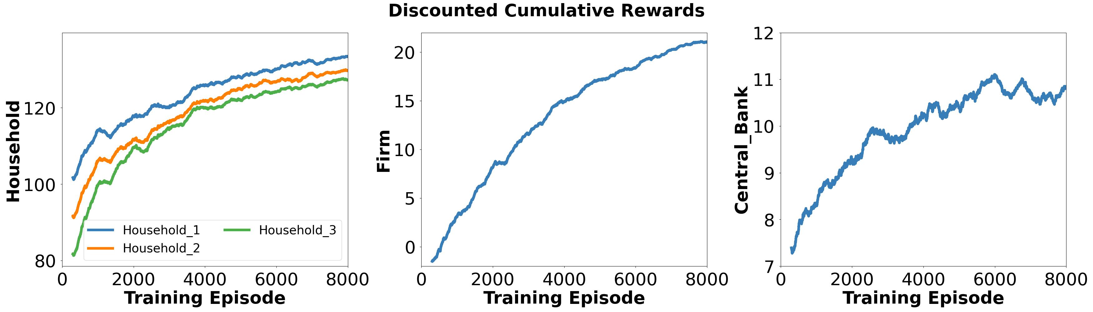
Figure 1: Training rewards without tax credits.

4.1 Multi-Agent Simulator

Our simulations are implemented based on a state-of-art multi-agent simulator called ABIDES (Byrd, Hybinette, and Balch 2019), and its OpenAI Gym extension called ABIDES-gym (Amrouni et al. 2021). It is a high-fidelity agent-based simulator used by practitioners and researchers in the financial domain (Vyetrenko et al. 2020; Dwarakanath, Vyetrenko, and Balch 2022). We adapt the simulator to model interactions between the economic agents described in Section 2 and enable multi-agent reinforcement learning using the Gym extension of the simulator.

4.2 Learning details

We describe the learning setup in more detail here.

• Households: We consider three households to demonstrate the efficacy of our models in this work although our setup is suitable for the use of many more. Each household’s consumption choices range from $0$ to $24$ units of goods in increments of $6$ units. Their labor choices range from $0$ to $960$ hours per quarter, in increments of $240$ hours. The proportion of consumption spending paid by tax credits can vary between $0$ and $1$, in units of $0.25$, subject to the constraint described in (9). The disutility of labor coefficient $\nu_{i}=0.5$ for all households. All households start with savings $m_{0,i}=0$.

• Firm: There is a single firm in the model. The firm’s choices for good prices range from $188$ to $456$ dollars, in increments of $67$ dollars. The wage choices for the firm range from $7.25$ to $56.87$ dollars per hour, in increments of $12.405$ dollars. The firm has labor efficiency $\alpha=0.67$, auto-regression coefficient $\rho=0.97$, shock standard deviation $\sigma=0.1$, and inventory risk coefficient $\chi=0.1$. The starting value of the exogenous production factor is $\epsilon_{0}=1$ with starting inventory $Y_{0}=0$.

• Central Bank: The central bank in the model can set interest rates that range from $0.25\%$ to $5.7\%$, in increments of $1.375\%$. The target inflation $\pi^{*}$ is $1.02$ and the coefficient for productivity $\lambda=1$.

• Government: The government chooses the income tax rate from a set of values: $0.10,0.12,0.22,$ $0.24,0.32,0.35,0.37$. The weighting coefficient $\theta$ for $\mathcal{H}_{t}$ in the government’s reward is set as $0.1$.

All agents have discount factor $\beta_{i,\mathbf{H}}=\beta_{\mathbf{F}}=\beta_{\mathbf{CB}}=\beta_{\mathbf{CB}}=0.99$. To ease learning, we normalize agent rewards so that their objectives are given as follows:

• Household:

  $$\sum_{t}\beta_{i,\mathbf{H}}^{t}u(c_{t,i},\frac{n_{t,i}}{\tilde{n}},\frac{m_{t+1,i}}{{\tilde{n}}\cdot\sum_{j}{\tilde{w}}};\gamma_{i},\nu_{i},\mu_{i}),$$

  where $\tilde{n}=480$ is the median labor hours in households’ action space, and $\tilde{w}=32.06$ is the median wage in the firm’s action space.

• Firm:

  $$\sum_{t}\beta_{\mathbf{F}}^{t} \left(\frac{p_{t}\sum_{i}c_{t,i}}{\tilde{p}\sum_{k}\tilde{c}}-\frac{w_{t}\sum_{i}n_{t,i}}{\tilde{w}\sum_{k}\tilde{n}}-\chi\frac{p_{t}Y_{t+1}}{\sum_{i}\exp(1)\tilde{p}\tilde{n}}\right)$$

  where $\tilde{p}=322$ is the median price in the firm’s action space, and $\tilde{c}=12$ is the median consumption in households’ action space.

• Central bank:

  $$\sum_{t}\beta_{\bf{CB}}^{t}\left(-\left(\pi_{t}-\pi^{\star}\right)^{2}+\lambda\left(\frac{y_{t}}{\tilde{y}}\right)^{2}\right),$$

  where $\tilde{y}=\left(\sum_{i}\tilde{n}\right)^{\alpha}$.

• Government:

  $$\sum_{t}\beta_{\mathbf{G}}^{t}\left(\theta\cdot\mathcal{H}_{t}^{\mathrm{norm}}+\sum_{i}\frac{1}{l_{t,i}}\cdot\frac{\kappa_{t+1,i}}{\sum_{k}{\tilde{p}}\cdot{\tilde{c}}}\right)$$

  where $\mathcal{H}_{t}^{\mathrm{norm}}$ is the sum of normalized rewards at $t$ across all households.

We use the Proximal Policy Optimization algorithm in the RLlib package to learn strategies for all reinforcement learning agents.

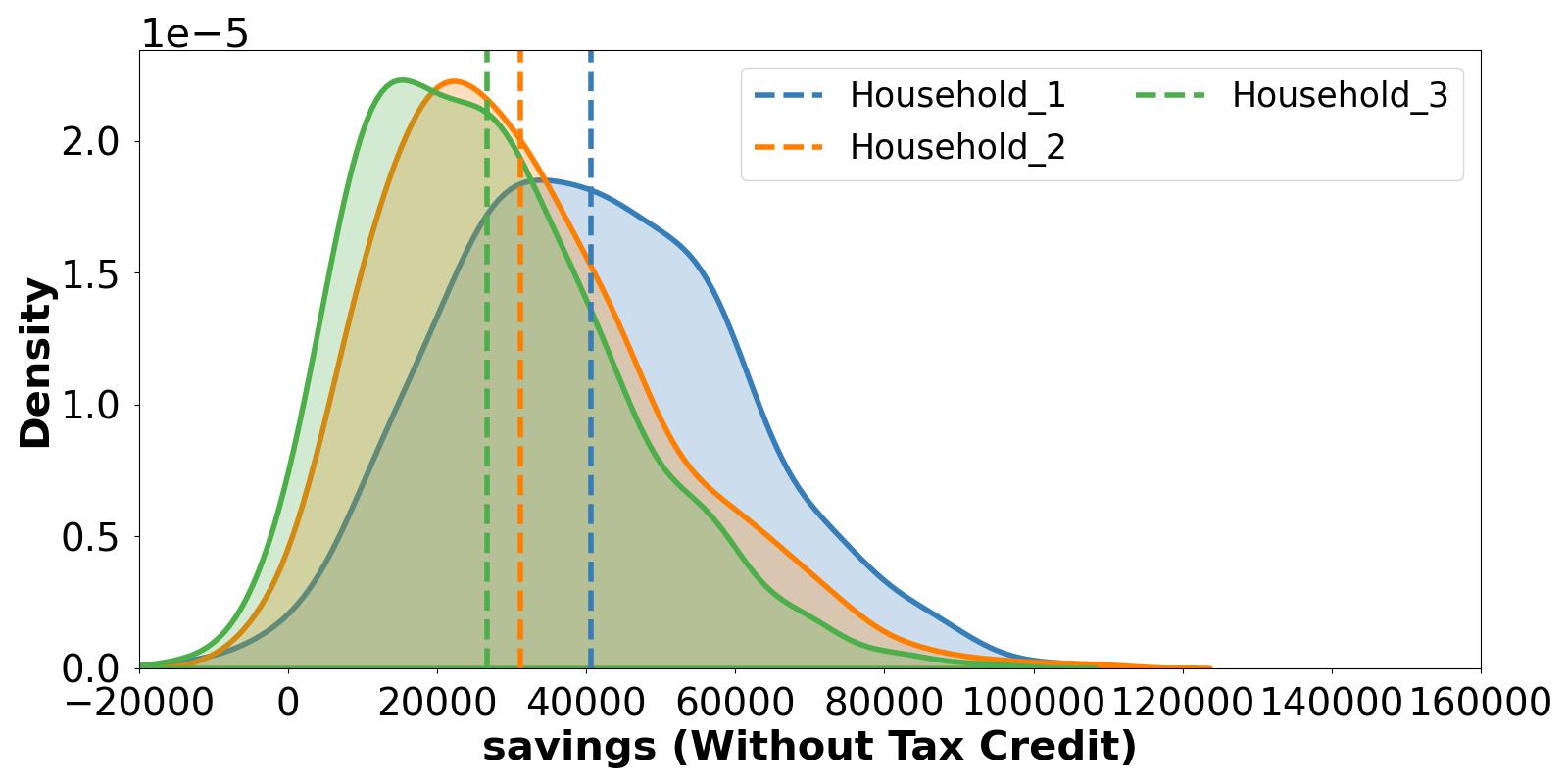
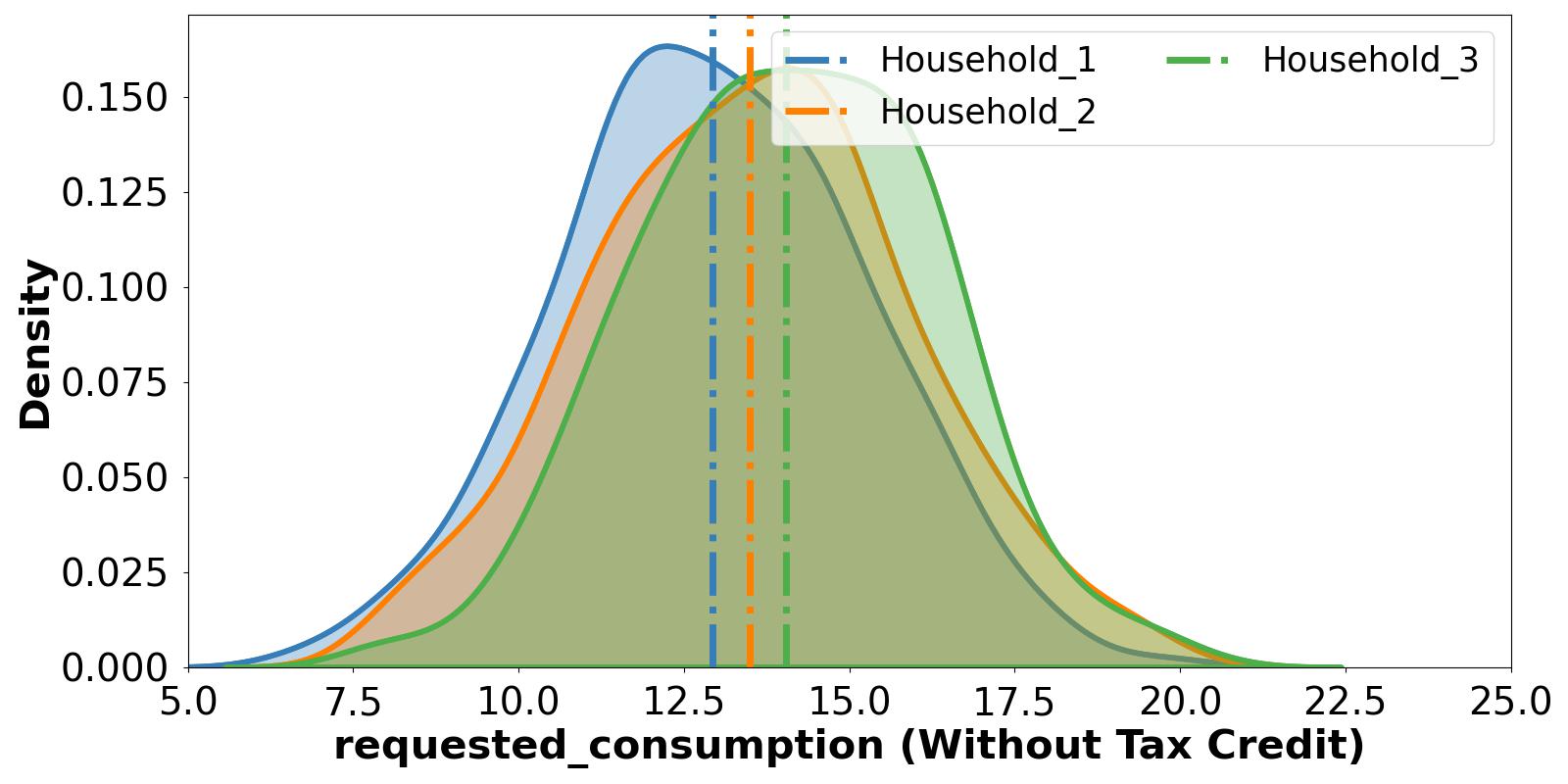
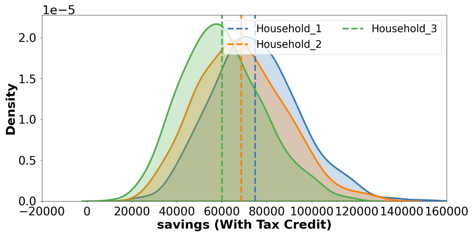
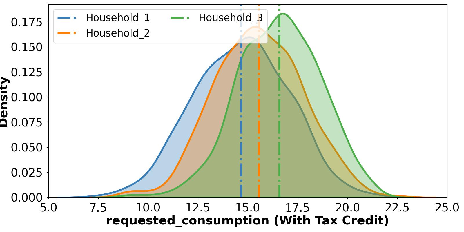
Figure 2: Transitory impact of tax credits on households. See the increase in savings and consumption for all households.

4.3 Transitory Impact of Tax Credits

To assess the transitory impact of tax credits on the economic system, we first train agent policies in the absence of tax credits. The trained policies are then tested in the presence of fixed tax credits to observe changes in strategies. Hence, for this experiment, we learn policies for three households, one firm, and the central bank, over a training horizon of three years so that $H=12$ quarters. To simulate households with different liquidities, recall that high-liquidity households tend to prioritize saving over spending. In contrast, low-liquidity households lean towards increased spending. To reflect this tendency, we set the parameters for isoelastic utility of the three households as $\gamma_{1}=0.1,\mu_{1}=0.4,\gamma_{2}=0.2,\mu_{2}=0.2,\gamma_{3}=0.3,\mu_{3}=0.1$ in order of decreased liquidity from Household 1 to Household 3. Throughout this process, we set distinct learning rates for each entity: $0.01$ for households, $0.005$ for the firm, and $0.001$ for the central bank. The discounted cumulative rewards during training are presented in Figure 1. It shows that the low-liquidity Household 3 has a lower reward compared to the high-liquidity Household 1.

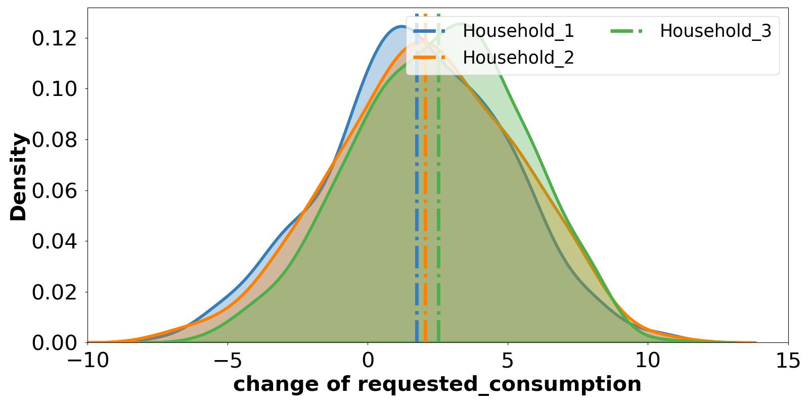
Figure 3: Change in requested consumption with tax credits. Household 3 with lowest liquidity sees the highest increase in consumption with tax credits.

During the testing phase, we play out the trained policies in experiments without and with a tax credit of $5000 per household per quarter. The distributions of household observables in test episodes are compared in Figure 2. It shows that Household 3 has the least savings and highest requested consumption, yielding the lowest liquidity. The impact of tax credits on households exhibits increased savings and consumption. Moreover, Figure 3 illustrates the change in average requested consumption per quarter with tax credit from that without. It shows that low-liquidity households experience a more significant boost in their requested consumption following the receipt of tax credits than higher liquidity households.

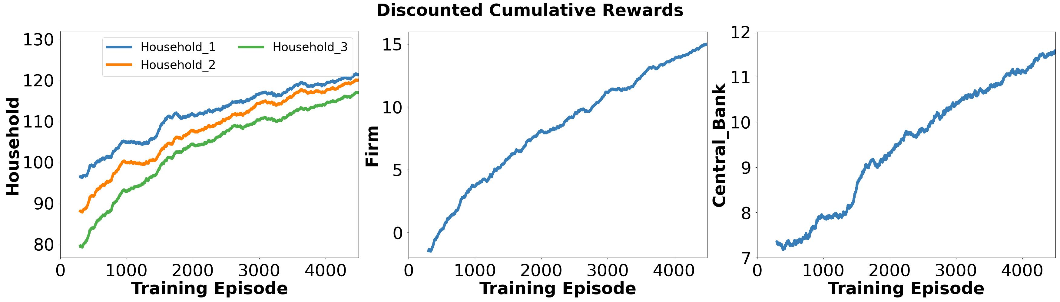
Figure 4: Training rewards with fixed tax credit distribution.

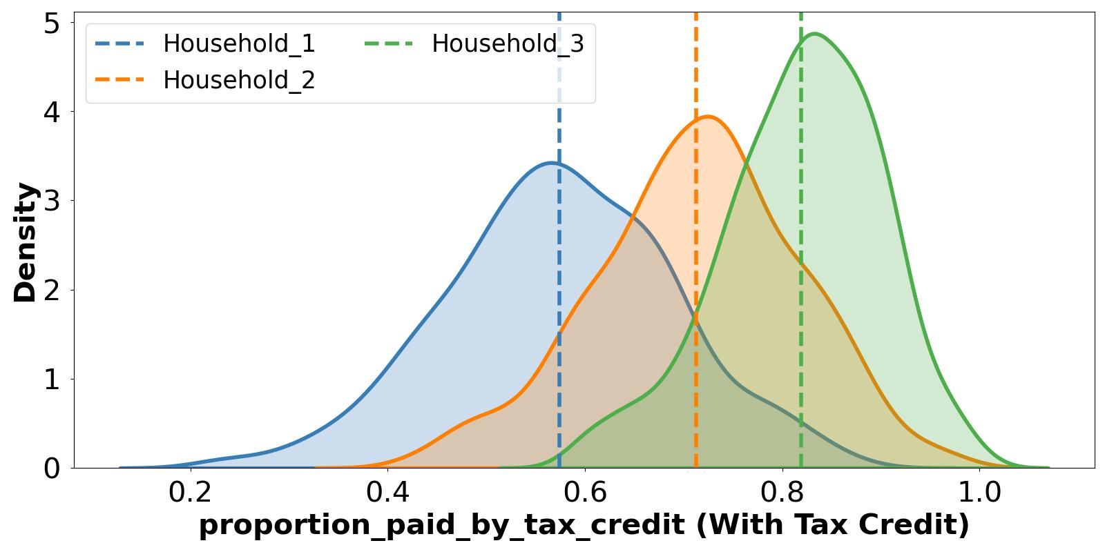
Figure 5: Spending patterns of fixed tax credits. Household 3 with lowest liquidity spends more of tax credit on consumption than others.

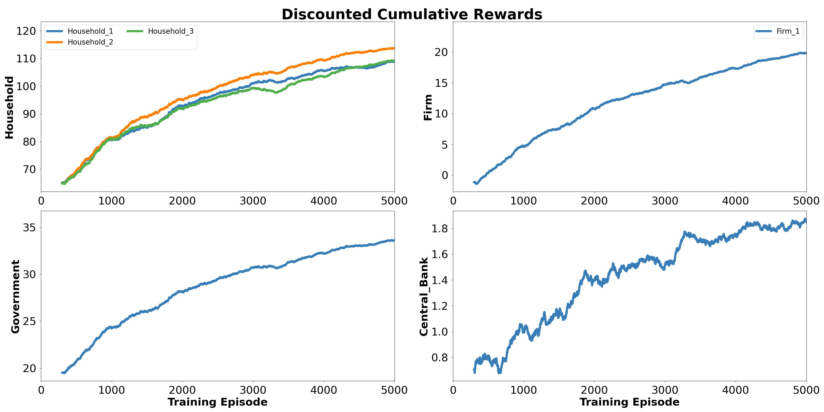
Figure 6: Training rewards with Government learning to distribute tax credits.

4.4 Impact of Tax Credits on Household Spending Patterns

Going a step further from studying the transitory impact of tax credits in the previous section, we now investigate the spending pattern of households following tax credit allocation. We employ the same agents as in Section 4.3 with the caveat that households have an additional action $\eta$ as described in Section 3.1. Additionally, all agents are now trained in the presence of a tax credit of $5000 per household per quarter. The learning rates employed are $0.002$ for households, $0.005$ for the firm, and $0.005$ for the central bank. The training rewards for each agent are shown in Figure 4. As before, Household 1 with the highest liquidity enjoys the highest reward among all households.

To evaluate the household spending patterns learned in the presence of tax credits, we play out the learned policies in test episodes to collect observations. Specifically, we plot the distribution of the new action $\eta$ depicting how households utilize tax credits towards consumption in Figure 5. The result demonstrates that low-liquidity households tend to expend a greater portion of their tax credits towards consumption spending than higher liquidity households. This observation is consistent with findings from the JP Morgan Chase report (Wheat, Deadman, and Sullivan 2022). Importantly, notice that with a fixed tax credit distribution scenario, low-liquidity households continue to receive less reward compared to their high-liquidity counterparts. This emphasizes the need to intelligently allocating collected tax revenue to households, especially those with lower liquidity, towards enhancing overall household welfare.

4.5 Strategy of Distributing Tax Credits

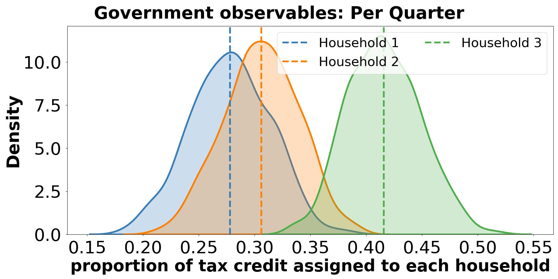
Figure 7: Government strategy for distributing tax credits. See that Household 3 with lowest liquidity receives a larger proportion of tax revenue as credits.

To improve the efficiency of tax credit distribution by the government, we integrate the government model proposed in Section 3.2 into the economic system setting in Section 4.3. We now learn policies for all agents in the economic system, with learning rates set at $0.002$ for households, $0.005$ for the firm, $0.005$ for the central bank, and $0.001$ for the government. The training rewards for each agent are represented in Figure 6. Unlike the findings in Figure 4 with fixed tax credit assignments, the rewards among households appear more consistent in Figure 6. This consistency in rewards signifies a more equitable distribution of resources among households, indicating the effectiveness of the integrated government model.

We test the trained agent policies to establish the efficacy of the tax credit distribution strategy. The simulation results illustrating the government’s distribution of tax credits to households are shown in Figure 7. The visualization shows the government’s tendency to allocate greater tax credits to households with lower liquidity. This strategic approach stands to substantially enhance the financial well-being of low-liquidity households, thereby fostering a more equitable economic landscape.

By incorporating the government model into the training process, we create a more comprehensive simulation that mirrors real-world policy implementation. This approach enables us to assess not only the effectiveness of tax credit distribution methods but also the influence of government policies on economic agents’ behaviors and decisions. Through this integrated analysis, we aim to provide valuable insights for policymakers, guiding them toward evidence-based decisions that can enhance the efficiency and fairness of tax credit distribution in the real economy.

5 Conclusion

We investigate the impact of tax credit allocation on the spending and saving behavior of diverse households in an economic system. We propose a multi-agent economic model encompassing heterogeneous households, a firm, central bank, and government. Each agent is equipped with reinforcement learning capabilities to adapt their strategies in response to others. By characterizing households by their liquidity (amount of savings versus consumption spending), we analyze their spending response to fixed and uniform tax credits. The outcomes of simulations distinctly highlight that households with lower liquidity tend to allocate a larger proportion of their tax credits toward consumption. This in turn affects their ability to save given necessary consumption spending with uniform credits. We subsequently propose a government strategy aimed at optimizing the distribution of tax credits to improve social welfare across households. Our simulation results demonstrate the effectiveness of this proposed strategy in ameliorating household inequalities, showing higher credit allocation to lower liquidity households.

Crucially, our work paves the way for the advancement of multi-agent reinforcement learning within economic models. The potential for exploration and expansion is vast. Enhancing the model’s complexity involves expanding the number of households and firms and developing efficient algorithms to train the multiple agent policies.

References

- Amrouni et al. (2021) Amrouni, S.; Moulin, A.; Vann, J.; Vyetrenko, S.; Balch, T.; and Veloso, M. 2021. ABIDES-gym: gym environments for multi-agent discrete event simulation and application to financial markets. In Proceedings of the Second ACM International Conference on AI in Finance, 1–9.
- Axtell and Farmer (2022) Axtell, R. L.; and Farmer, J. D. 2022. Agent-based modeling in economics and finance: Past, present, and future. Journal of Economic Literature.
- Benhabib, Schmitt-Grohé, and Uribe (2001) Benhabib, J.; Schmitt-Grohé, S.; and Uribe, M. 2001. Monetary policy and multiple equilibria. American Economic Review, 91(1): 167–186.
- Blinder et al. (2008) Blinder, A. S.; Ehrmann, M.; Fratzscher, M.; De Haan, J.; and Jansen, D.-J. 2008. Central bank communication and monetary policy: A survey of theory and evidence. Journal of economic literature, 46(4): 910–945.
- Blundell et al. (2000) Blundell, R.; Duncan, A.; McCrae, J.; and Meghir, C. 2000. The labour market impact of the working families’ tax credit. Fiscal studies, 21(1): 75–104.
- Buşoniu, Babuška, and De Schutter (2010) Buşoniu, L.; Babuška, R.; and De Schutter, B. 2010. Multi-agent reinforcement learning: An overview. Innovations in multi-agent systems and applications-1, 183–221.
- Byrd, Hybinette, and Balch (2019) Byrd, D.; Hybinette, M.; and Balch, T. H. 2019. Abides: Towards high-fidelity market simulation for ai research. arXiv preprint arXiv:1904.12066.
- Chen et al. (2021) Chen, M.; Joseph, A.; Kumhof, M.; Pan, X.; Shi, R.; and Zhou, X. 2021. Deep reinforcement learning in a monetary model. arXiv preprint arXiv:2104.09368.
- Cobb and Douglas (1928) Cobb, C. W.; and Douglas, P. H. 1928. A theory of production. American Economic Association.
- Curry et al. (2022) Curry, M.; Trott, A.; Phade, S.; Bai, Y.; and Zheng, S. 2022. Analyzing Micro-Founded General Equilibrium Models with Many Agents using Deep Reinforcement Learning. arXiv preprint arXiv:2201.01163.
- Dosi and Roventini (2019) Dosi, G.; and Roventini, A. 2019. More is different… and complex! the case for agent-based macroeconomics. Journal of Evolutionary Economics, 29: 1–37.
- Dwarakanath, Vyetrenko, and Balch (2022) Dwarakanath, K.; Vyetrenko, S.; and Balch, T. 2022. Equitable Marketplace Mechanism Design. In Proceedings of the Third ACM International Conference on AI in Finance, 232–239.
- Ellwood (2000) Ellwood, D. T. 2000. The impact of the earned income tax credit and social policy reforms on work, marriage, and living arrangements. National tax journal, 53(4): 1063–1105.
- Evans and Honkapohja (2005) Evans, G. W.; and Honkapohja, S. 2005. Policy interaction, expectations and the liquidity trap. Review of Economic Dynamics, 8(2): 303–323.
- Haldane and Turrell (2019) Haldane, A. G.; and Turrell, A. E. 2019. Drawing on different disciplines: macroeconomic agent-based models. Journal of Evolutionary Economics, 29: 39–66.
- Hill, Bardoscia, and Turrell (2021) Hill, E.; Bardoscia, M.; and Turrell, A. 2021. Solving heterogeneous general equilibrium economic models with deep reinforcement learning. arXiv preprint arXiv:2103.16977.
- Hinterlang and Tänzer (2021) Hinterlang, N.; and Tänzer, A. 2021. Optimal monetary policy using reinforcement learning. Deutsche Bundesbank Discussion Paper.
- Hu, Wellman et al. (1998) Hu, J.; Wellman, M. P.; et al. 1998. Multiagent reinforcement learning: theoretical framework and an algorithm. In ICML, volume 98, 242–250.
- Kaplan, Moll, and Violante (2018) Kaplan, G.; Moll, B.; and Violante, G. L. 2018. Monetary policy according to HANK. American Economic Review, 108(3): 697–743.
- Krusell and Smith (1998) Krusell, P.; and Smith, A. A., Jr. 1998. Income and wealth heterogeneity in the macroeconomy. Journal of political Economy, 106(5): 867–896.
- Littman (1994) Littman, M. L. 1994. Markov games as a framework for multi-agent reinforcement learning. In Machine learning proceedings 1994, 157–163. Elsevier.
- Liu et al. (2022) Liu, Z.; Lu, M.; Wang, Z.; Jordan, M.; and Yang, Z. 2022. Welfare maximization in competitive equilibrium: Reinforcement learning for markov exchange economy. In International Conference on Machine Learning, 13870–13911. PMLR.
- Nowé, Vrancx, and De Hauwere (2012) Nowé, A.; Vrancx, P.; and De Hauwere, Y.-M. 2012. Game theory and multi-agent reinforcement learning. Reinforcement Learning: State-of-the-Art, 441–470.
- Sinitskaya and Tesfatsion (2015) Sinitskaya, E.; and Tesfatsion, L. 2015. Macroeconomies as constructively rational games. Journal of Economic Dynamics and Control, 61: 152–182.
- Svensson (2020) Svensson, L. E. 2020. Monetary policy strategies for the Federal Reserve. Technical report, National Bureau of Economic Research.
- Vyetrenko et al. (2020) Vyetrenko, S.; Byrd, D.; Petosa, N.; Mahfouz, M.; Dervovic, D.; Veloso, M.; and Balch, T. 2020. Get real: Realism metrics for robust limit order book market simulations. In Proceedings of the First ACM International Conference on AI in Finance, 1–8.
- Wheat, Deadman, and Sullivan (2022) Wheat, C.; Deadman, E.; and Sullivan, D. M. 2022. How families used the advanced Child Tax Credit. Technical report, JPMorgan Chase Institute.
- Zheng et al. (2022) Zheng, S.; Trott, A.; Srinivasa, S.; Parkes, D. C.; and Socher, R. 2022. The AI Economist: Taxation policy design via two-level deep multiagent reinforcement learning. Science Advances, 8(18): 2607.