Detecting influential observations in single-index models with metric-valued response objects

Abstract

Regression with random data objects is becoming increasingly common in modern data analysis. Unfortunately, like the traditional regression setting with Euclidean data, random response regression is not immune to the trouble caused by unusual observations. A metric Cook’s distance extending the classical Cook’s distances of Cook, (1977) to general metric-valued response objects is proposed. The performance of the metric Cook’s distance in both Euclidean and non-Euclidean response regression with Euclidean predictors is demonstrated in an extensive experimental study. A real data analysis of county-level COVID-19 transmission in the United States also illustrates the usefulness of this method in practice.

Keywords: Metric Cook’s Distance, Influential observations, Distributional responses, Fréchet regression

1 Introduction

Regression beyond the traditional Euclidean space has attracted much attention lately. To accommodate the complex structure of new data types, novel techniques have been introduced to bypass the usual operations on vector spaces. Faraway, (2014) proposed to use multidimensional scaling to obtain scores from the distance matrices of the random predictor and response objects and then apply linear regression to the scores. In particular, for regressing random response objects on Euclidean predictors, Petersen and Müller, (2019) introduced Fréchet regression, which can accommodate responses in the space of probability distributions, covariance matrices, and spheres. The regression of general metric-valued responses on Euclidean predictors is the focus of this study.

Let $Y$ be a random response in the compact metric space $(\Omega_{Y},d)$ equipped with a metric $d:\Omega_{Y}\times\Omega_{Y}\to\mathbb{R}$. Denote the $p$-dimensional predictor as ${\bf X}\in\mathbb{R}^{p}$. For a random object $({\bf X},Y)\in\mathbb{R}^{p}\times\Omega_{Y}$, let $F_{XY}$ be the joint distribution of ${\bf X}$ and $Y$, and assume the conditional distributions $F_{Y|X}$ and $F_{X|Y}$ exist and are well-defined. The Fréchet regression function of $Y$ on ${\bf X}$ is the conditional Fréchet mean defined by Petersen and Müller, (2019) as

$$m_{\bigoplus}({\bm{x}})=\operatorname*{arg\,min}_{\omega\in\Omega_{Y}}M_{\bigoplus}(.,{\bm{x}}),$$ (1)

where $M_{\bigoplus}(.,{\bm{x}})=\operatorname{E}[d^{2}(Y,.)|{\bf X}={\bm{x}}]$ is the conditional Fréchet function .

Firstly, we note that the Fréchet regression function in (1) is not immune to the problems commonly encountered in traditional regression such as high predictor dimensionality, outliers, and influential observations. For dealing with large $p$, existing sufficient dimension reduction methods such as ordinary least square (OLS;Li and Duan, (1989)) and sliced inverse regression (SIR; Li, (1991)) have been extended to accommodate non-Euclidean responses. See for example, Fréchet dimension reduction (Zhang et al., (2021)), Fréchet kernel sliced inverse regression (Dong and Wu, (2022)), and surrogate-assisted dimension reduction (Soale and Dong, (2023)).

Secondly, the sensitivity of OLS, SIR, and other SDR methods to extreme observations in the Euclidean response case are well-known in the SDR literature [Gather et al., (2002); Prendergast, (2008); Chen et al., (2022)]. For instance, in the multiple linear regression setting, extreme observations can significantly change the OLS estimate. A powerful tool for diagnosing these influential observations is to use Cook’s distances (Cook, (1977)). For single-index models, Prendergast, (2008) proposed a similar leave-one-out method based on multiple correlation coefficient for diagnosing influential observations. However, neither of these methods can be directly applied to regression with non-Euclidean data, which restricts their implementation in this emerging random objects regression. So far, to the best of our knowledge, there is no method addressing the effects of unusual observations and the sensitivity of these new sufficient dimension reduction techniques to influential data objects in the literature. In this paper, we fill this gap by introducing a metric Cook’s distance, which can diagnose influential observations in regression with general metric-valued responses on Euclidean predictors.

It is important to note that some of the responses in non-Euclidean spaces may not have an algebraic structure. Therefore, operations on vector spaces such as inner products are not guaranteed. However, since we can at least compute distances in every compact metric space, we can overcome this challenge by using a surrogate response based on the response metric, which is generalizable. The basic idea is to first represent the response objects as a pairwise distance matrix using the appropriate metric and then estimate the underlying low-dimensional representation using metric multidimensional scaling [Kruskal, (1964); Kruskal and Wish, (1978)]. The leading score, which is a scalar is then used as the surrogate response to calculate the regular Cook’s distances to diagnose potential influential observations. Thus, we call our proposal the metric Cook’s distance. We also show through extensive simulation studies, how trimming the influential observations can lead to improved estimates. Beyond obtaining better estimates, the metric Cook’s distance also comes in handy in studies where the researcher’s goal is to detect anomalies in the data.

We organize the rest of the paper as follows. Section 2 describes the method and sample-level estimation of the metric Cook’s distances. In Section 3 we show the performance of our proposal through extensive experimental studies. A real application of the metric Cook’s distance on COVID-19 transmissions in the United States to detect counties with influential transmission rates is given in Section 4. The concluding remarks are given in Section 5. All proofs and technical details are relegated to the appendix.

2 Metric Cook’s Distance

Suppose there exist a mapping $f:\mathbb{R}^{p}\mapsto\Omega_{Y}$, such that for a random object $({\bf X},Y)$, we have the single-index model:

$$Y=f(\beta^{\top}{\bf X},\epsilon),$$ (2)

where $f$ is some unknown link function, $\beta\in\mathbb{R}^{p}$ is such that $\lVert\beta\rVert_{2}=1$, and $\operatorname{E}(\epsilon|{\bf X})=0$ almost surely to allow for dependence between $\epsilon$ and ${\bf X}$. Our goal is to estimate the subspace that contains $\beta$ without imposing stringent conditions on $f$, which can be achieved by using sufficient dimension reduction (SDR) techniques.

2.1 Surrogate ordinary least squares

Based on model 2, by definition,

$$Y\perp\!\!\!\perp{\bf X}|\beta^{\top}{\bf X},$$ (3)

where $\perp\!\!\!\perp$ means statistical independence. $\beta$ is the dimension reduction subspace and is not identifiable. However, under mild conditions, the intersection of all such subspaces exists and is unique, and is called the central space for the regression of $Y$ on ${\bf X}$, denoted by ${\mathcal{S}}_{Y|{\bf X}}$. The central space is given by ${\mathcal{S}}_{Y|{\bf X}}=\mathrm{span}(\beta)$. See [Cook, (1996); Yin et al., (2008)] for the existence and uniqueness of the central space.

In non-Euclidean spaces, because $Y$ may not have an algebraic structure, we may not be able to estimate $\beta$ with the existing methods that use $Y$ directly. We circumvent this problem by using a Euclidean surrogate of $Y$ which preserves the distances between the original response objects. The upcoming lemma shows that we can recover an unbiased estimate of ${\mathcal{S}}_{Y|{\bf X}}$ using regression based on the surrogate.

Lemma 1.

Suppose $\tilde{Y}$ is a random copy $Y$ and let $\phi$ be some measurable function. Then $\mathcal{S}_{\phi(Y,\tilde{Y})|{\bf X}}\subseteq{\mathcal{S}}_{Y|{\bf X}}$.

By Lemma 1, we can use the regression of $\phi(Y,\tilde{Y})$ versus ${\bf X}$ to estimate the ${\mathcal{S}}_{Y|{\bf X}}$. We call $\phi(Y,\tilde{Y})$ the surrogate response, denoted by $S^{Y}$. The next hurdle is to determine the appropriate choice of $\phi(.)$. Notice that since $Y\in(\Omega_{Y},d)$, we are guaranteed that distances can be computed on $\Omega_{Y}$. Therefore, we choose $S^{Y}=g[d(Y,\tilde{Y})]$, where $d$ is some appropriate metric and $g$ is some function. We then proceed to estimate $\beta$, using the existing classical SDR methods. While there are many methods that can be employed to find $\beta$, we are specifically interested in the ordinary least squares, which requires the following assumptions.

Assumption 1.

We assume the function $f$ is monotone.

Assumption 2.

We assume that $\operatorname{E}({\bf X}|\beta^{\top}{\bf X})$ is a linear function of $\beta^{\top}{\bf X}$.

Assumptions 1 allows us to employ first-moment sufficient dimension reduction methods such as OLS or SIR. These methods are known to perform poorly when the link function is symmetric. Assumption 2 is the linear conditional mean (LCM) assumption, which is famous in the sufficient dimension reduction literature. LCM is shown to be satisfied when the distribution of ${\bf X}$ is elliptical and where it does not hold, we can transform ${\bf X}$ to achieve ellipticity, see [Eaton, (1986); Li, (2018)].

Theorem 1.

Suppose Assumptions 1 and 2 are satisfied. If $\bm{\Sigma}=\text{Var}({\bf X})$ is invertible, then

$$\bm{\Sigma}^{-1}\bm{\Sigma}_{XS^{Y}}\in{\mathcal{S}}_{Y|{\bf X}},$$ (4)

where $\bm{\Sigma}=\text{Var}({\bf X})$, $\bm{\Sigma}_{XS^{Y}}=\text{Cov}({\bf X},S^{Y})$.

Notice that $\bm{\Sigma}^{-1}\bm{\Sigma}_{XS^{Y}}$ is the ordinary least squares estimator for the regression of $S^{Y}$ versus ${\bf X}$.

2.2 Estimation in finite sample

The metric Cook’s distance estimation involves two steps. In the first step, we find the surrogate response, and the second step involves calculating Cook’s distances for the regression between the surrogate response and the predictor.

2.2.1 Finding $S^{Y}$ via metric multidimensional scaling (MMDS)

Metric multidimensional scaling is a common dimension reduction technique [Kruskal, (1964); Kruskal and Wish, (1978)]. Let $({\bm{x}}_{1},y_{1}),\ldots,({\bm{x}}_{n},y_{n})$ denote a random sample of $({\bf X},Y)$. We compute the $n\times n$ pairwise distance matrix ${\bf D}^{Y}$ such that ${\bf D}^{Y}_{ij}=d(y_{i},y_{j})$ for $i,j=1,\ldots,n$. For instance, if $Y\in\mathbb{R}$, ${\bf D}^{Y}_{ij}=|y_{i}-y_{j}|,\ i,j=\{1,\ldots,n\}$. Similarly, for $Y\in\mathbb{R}^{q},q\geq 2$, we may use ${\bf D}^{Y}_{ij}=\lVert y_{i}-y_{j}\rVert_{2}$. If $Y$ is the collection of probability distributions, we follow the lead of Petersen and Müller, (2019) and use the Wasserstein metric. In effect, the choice of distance metric depends on the space of the response distributions. The decision is left to the discretion of the practitioner where there are multiple choices for $d$.

Regardless of the response space, ${\bf D}^{Y}$ is expected to be a symmetric matrix of $\mathbb{R}^{n}$ whose diagonal elements are all zeros. Therefore, ${\bf D}^{Y}$ is a dependent matrix. By the theory of classical multidimensional scaling, we estimate the factor scores from the singular value decomposition of the double-centered squared distances ${\bf D}^{Y}_{2}$. Let

$$M=-\cfrac{1}{2}\bm{Q}_{n}{\bf D}^{Y}_{2}\bm{Q}_{n},$$ (5)

where $\bm{Q}_{n}={\bf I}_{n}-\cfrac{1}{n}\bm{J}_{n}$, ${\bf I}_{n}$ is an $n\times n$ identity matrix, and $\bm{J}_{n}$ is an $n\times n$ matrix of all 1’s. Then $M$ is positive semi-definite with a spectral decomposition $M={\bf V}\bm{\Lambda}{\bf V}^{\top}$, where $\bm{\Lambda}=diag\{\lambda_{1},\ldots,\lambda_{k}\}$ with $\lambda_{1}\geq\lambda_{2}\ldots\geq\lambda_{k}>0$, ${\bf V}^{\top}{\bf V}={\bf I}_{k}$.

The factor scores ${\bf V}\Lambda^{1/2}\in\mathbb{R}^{n\times k}$ will also have a Euclidean distance matrix ${\bf D}^{Y}$. Therefore, we let $S^{Y}={\bf V}\Lambda^{1/2}$. Ideally, we would have to determine the number of scores to retain. However, since we focus only on single-index models, we choose the first score, which corresponds to the leading eigenvalue of $M$ as $S^{Y}$. It is easier to show that for scalar Euclidean response, $S^{Y}$ is simply a scaled $Y$.

Suppose $Y\in\mathbb{R}^{n\times q}$, then $Y$ can be factored as

$$Y=USV^{\top}=\sum_{i=1}^{q}\sigma_{i}u_{i}v_{i}^{\top},$$ (6)

where $U=[u_{1}\ldots u_{q}]\in\mathbb{R}^{n\times q}$ and $V=[v_{1}\ldots v_{q}]\in\mathbb{R}^{q\times q}$ are orthonormal matrices, and $S\in\mathbb{R}^{q\times q}$ is diagonal with entries $\sigma_{1}\geq\sigma_{2},\ldots\geq\sigma_{q}\geq 0$. If $Y$ has rank 1, then we have $Y\approx\sigma_{1}u_{1}v_{1}^{\top}$. The matrix $M$ in (5) can be expressed as the gram matrix $YY^{\top}=\sigma^{2}u_{1}u_{1}^{T}$. This implies that $u_{1}$ is also the eigenvector of $YY^{\top}$ corresponding to the leading eigenvalue, which is $\sigma_{1}^{2}$. Therefore, $S^{Y}$ yields the best approximation of $Y$. For a scalar $Y$, $\sigma_{1}=\lVert Y\rVert_{2}$, $u_{1}=Y/\lVert Y\rVert_{2}$, and $v_{1}=1$. Hence, using $S^{Y}$ is essentially $Y$ as demonstrated later in Example 1.

2.2.2 Cook’s Distance

The metric Cook’s Distance is based on the OLS estimate of the regression between $S^{Y}$ versus ${\bf X}$. The calculation of the Cook’s distances involves the intercept estimate, which is incorporated into (4) by augmenting the ${\bf X}$ matrix with a vector of 1’s. That is, we let $\tilde{\bf X}=[1,{\bf X}]$ with the corresponding parameter estimate $\tilde{\beta}=\tilde{\bm{\Sigma}}^{-1}\bm{\Sigma}_{\tilde{X}S^{Y}}$, where $\tilde{\bm{\Sigma}}=\text{Var}(\tilde{\bf X})$. Denote $\tilde{\beta}_{(-i)}$ as the OLS estimate when the $i$th observation is left out. Then the $i$th Cook’s distance is defined as

$$\delta_{i}=\cfrac{(\tilde{\beta}_{(-i)}-\tilde{\beta})^{\top}(\tilde{\bf X}^{\top}\tilde{\bf X})(\tilde{\beta}_{(-i)}-\tilde{\beta})}{(p+1)s^{2}}=\left[\cfrac{(S^{Y}_{i}-\tilde{\beta}^{\top}\tilde{\bf X}_{i})^{2}}{(p+1)s^{2}}\right]\cfrac{h_{ii}}{(1-h_{ii})^{2}},$$ (7)

where $s^{2}=\cfrac{1}{n-p-1}\displaystyle\sum_{i=1}^{n}(S^{Y}_{i}-\tilde{\beta}^{\top}\tilde{\bf X}_{i})^{2}$ and $0\leq h_{ii}\leq 1$ is the $i$th leverage point.

High values of $\delta_{i}$ indicate that the $i$th observation is likely influential. While there is no standard threshold for classifying an observation as influential, several cutoffs have been suggested in the literature. Here, we use $4/(n-p-1)$.

The estimation is summarized in the algorithm that follows.

Algorithm 1 Metric Cook’s Distance

1:Input: Predictor ${\bf X}$ as $(n\times p)$ matrix, response $Y_{n}=\{y_{1},\ldots,y_{n}\}$ as list

2:Compute $n\times n$ matrix ${\bf D}_{n}$, ${\bf D}_{n}[i,j]\leftarrow d(y_{i},y_{j}),\ \forall i,j=1\ldots,n$

3:Compute the classical multidimensional scaling factor scores based on ${\bf D}_{n}$

4:Set the score corresponding to the leading eigenvalue in (3) as $S_{Y}$

5:Compute the Cook’s distances for the linear regression of $S_{Y}$ versus ${\bf X}$

3 Experimental Studies

In this section, we will demonstrate the performance of the metric Cook’s distance on synthetic data. We will consider responses in three different metric spaces, starting from the Euclidean space. While for scalar responses there is very little incentive to use the metric Cook’s distance, our proposal is incredibly useful in reduced-rank regression.

3.1 Response in the Euclidean space

In this response space, we explore single-index scalar response models and rank 1 vector response models. The same data generation process for the predictors is used in both scenarios. We fix the sample size $n=100$ and set $p=10$, and then generate the predictor ${\bm{x}}\sim N(\bm{0},\bm{\Sigma})$, where $\bm{\Sigma}_{ij}=0.5^{|i-j|}$.

Example 1 (Scalar response).

Let $\beta=(1,1,0,\ldots,0)\in\mathbb{R}^{p}$ and generate the response as

$$y_{i} =0.5+\beta^{\top}{\bm{x}}_{i}+\epsilon_{i},$$

$$\epsilon_{i} \overset{i.i.d.}{\sim}\begin{cases}N(0,0.5^{2}),\ i=\{1,\ldots,n\}\backslash\{10,15\}\\ N(5,2^{2}),\ i=\{10,15\}\end{cases}.$$

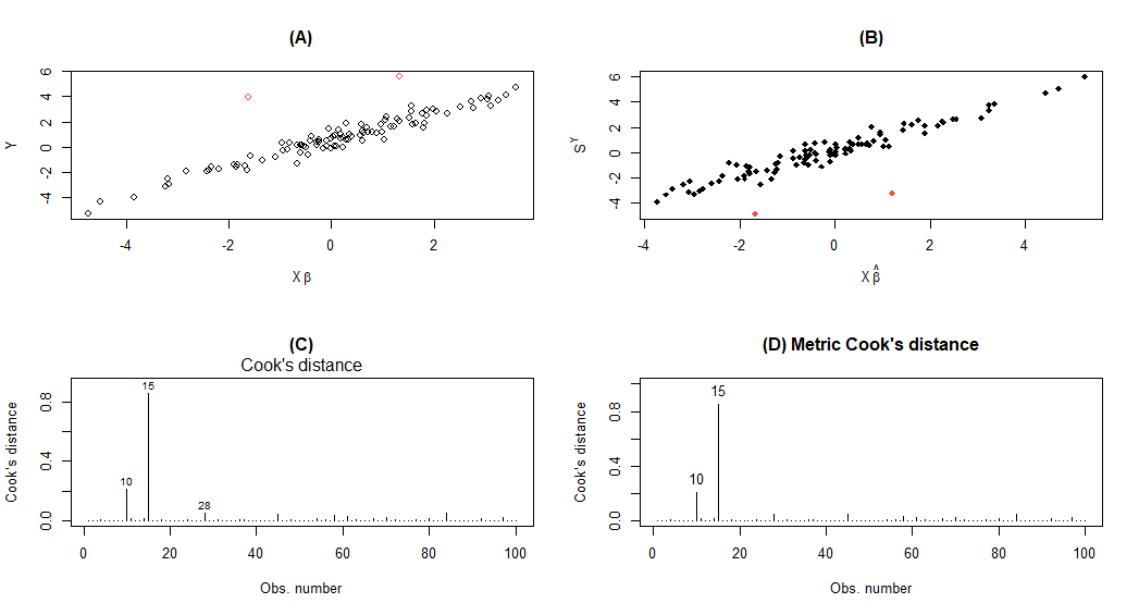
The 10th and 15th observations are outliers. As expected, the Cook’s distance plot for the regression with $y$ flagged these observations as potential influential observations as seen in exhibit (C) in Figure 1. However, as demonstrated in exhibit (D), Cook’s distance based on the surrogate response $S^{Y}$ mirrors what we observed in (C). This suggests that the metric Cook’s distance is equally as good when the response is a scalar. Moreover, the scatter plots appear to recover the same direction, albeit the direction in (B) is reversed. This result is not surprising as $S^{Y}$ is essentially $Y$.

Figure 1: Exhibits (A) and (B) show the respective scatter plots based on $Y$ and $S^{Y}$ with the outliers displayed in red. The corresponding Cook’s distance plots are given in (C) and (D).

Example 2 (Reduced-rank vector response).

Let $\beta=(1,-1,0,\ldots,0)\in\mathbb{R}^{p}$ and $\eta$ be a random 1-by-2 orthogonal matrix. The response is generated as

$$\bm{y} =\sin({\bf B}^{\top}{\bm{x}}_{i})+\bm{\epsilon}_{i},$$

$${\bf B} =\beta\eta\in\mathbb{R}^{p\times 2}\text{ with }\mathrm{rank}({\bf B})=1,$$

$$\bm{\epsilon}_{i} =(\epsilon_{i1},\epsilon_{i2})\sim N(\bm{0},\bm{\Sigma}_{\epsilon}),\text{ with }\bm{\Sigma}_{\epsilon}=\begin{bmatrix}1&0.7\\ 0.7&1\end{bmatrix},\text{ for }i=\{1,\ldots,n\}\backslash\{10,15\},$$

$$\epsilon_{i1} \overset{i.i.d.}{\sim}N(5,2^{2}),\text{ for }i=10,$$

$$\epsilon_{i2} \overset{i.i.d.}{\sim}N(-5,2^{2}),\text{ for }i=15.$$

Figure 2: Scatter plot of the bivariate response versus the true direction $\beta^{\top}{\bm{x}}$

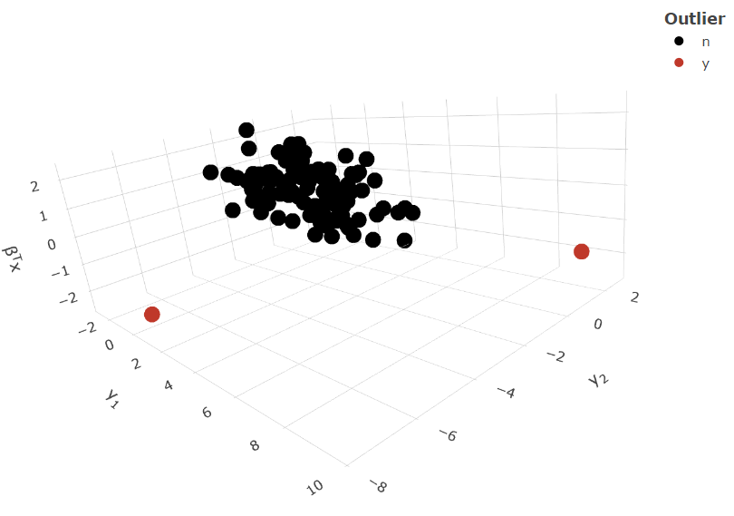
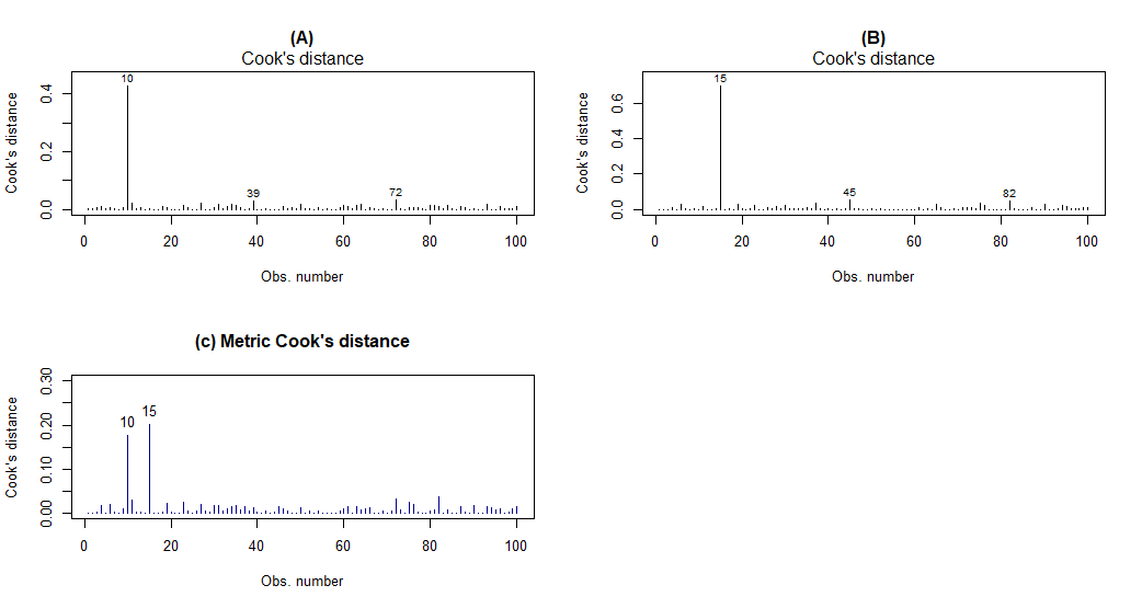
The scatter plot in Figure 2 shows two clear outliers, one each from the two responses. We expect the metric Cook’s distance to have no difficulty in detecting these unusual observations. In Figure 3, we have two different Cook’s distance estimates based on the regression of $\bm{y}$ versus ${\bm{x}}$ in exhibits (A) and (B). This is because implementing OLS with a vector response is equivalent to finding the estimates for the individual responses and stacking them together in columns. Thus, OLS does not make use of the dependence information between the responses although they are moderately correlated. In contrast, the surrogate response takes the dependence in $\bm{y}$ into account and is able to detect the extreme observations from the single surrogate responses as illustrated in exhibit (C).

Figure 3: Exhibits (A) and (B) are based on $Y$ while exhibits (C) is based on $S^{Y}$

3.2 Response in the space of probability distributions

We turn our focus now on univariate distributional responses. For this class of response objects, we used the Wasserstein metric to find the pairwise distances. Let $F_{1}(.)$ and $F_{2}(.)$ be the cumulative distribution functions of some two distributions. We define the quadratic Wasserstein distance as

$$W_{2}(F_{1},F_{2})=\sqrt{\int_{0}^{1}\big{(}F_{1}^{-1}(t)-F_{2}^{-1}(t)\big{)}^{2}dt}.$$ (8)

Example 3.

For this response space, our data generation process takes the lead from Zhang et al., (2021) and Soale and Dong, (2023). Fix $(n,p)=(100,10)$ and let $\beta_{1}=(1,-1,0,\ldots,0)/\sqrt{2}\in\mathbb{R}^{p}$. Generate the data as follows.

$${\bm{x}}_{i} \in\mathbb{R}^{p}\overset{i.i.d.}{\sim}\ Unif(0,1),\ i=1,\ldots,n,$$

$$y_{i} \in\mathbb{R}^{50}\overset{i.i.d.}{\sim}Unif(-5*|\beta^{\top}{\bm{x}}_{i}|,5*|\beta^{\top}{\bm{x}}_{i}|),\ i=\{1,\ldots,n\}\backslash\{10,15\},$$

$$y_{i} \in\mathbb{R}^{50}\overset{i.i.d.}{\sim}\exp(|\beta^{\top}{\bm{x}}_{i}|),\text{ for }i=10,$$

$$y_{i} \in\mathbb{R}^{50}\overset{i.i.d.}{\sim}0.5*N(0,|\beta^{\top}{\bm{x}}_{i}|)+0.5*N(\beta^{\top}{\bm{x}}_{i},5),\text{ for }i=15.$$

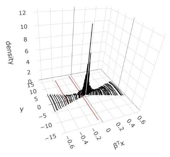
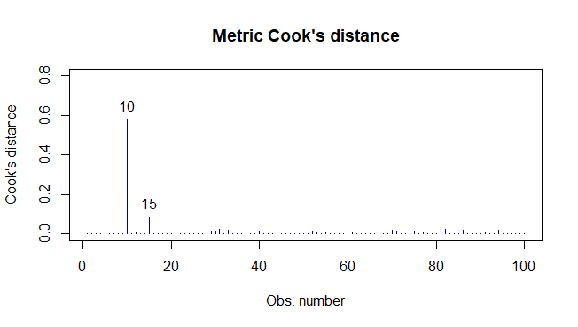
The 10th and 15th response distributions in red differ significantly in shape and spread from the remaining distributions in black, and we expect the Wasserstein metric to be able to capture the difference. The 3D plot of densities versus the true predictor on the left in Figure 4 illustrates this. The plot on the right in Figure 4, accurately detects these two unusual distributions as influential.

Figure 4: Influential observations for distributional response regression based on $S^{Y}$

3.3 Functional response

To compute the distance between any two functional responses, we first find their discrete Fourier transform (DFT). DFT maps a given sequence to a low-dimensional space and also reveals the periodicities and their relative strengths at the periodic components. Next, we compute the Euclidean distance between the modulus of the Fourier coefficients. Details about this distance metric can be found in Agrawal et al., (1993). For $T$ time points, we use $\lfloor{T/2}\rfloor+1$ coefficients to compute the distances. An alternative metric for this type of response is the Fréchet distance, which was used in Faraway, (2014).

Example 4.

For this example, we simulate functional responses with varying intercepts over time but fixed predictor effects across time. Fix $(n,p)=(100,10)$ and let $\beta_{1}^{\top}=(1,-1,0,\ldots,0)/\sqrt{2}\in\mathbb{R}^{p}$. The data generation process is as follows.

$$t \in\mathbb{R}^{30}\sim Unif(0,10),$$

$$\alpha_{0}(t) =10\cos(\pi+\pi t/5),$$

$$y_{i}(t) =\alpha_{0}(t)+5[\sin(\beta_{1}^{\top}{\bm{x}}_{i})]\phi(t)+\epsilon_{i}(t),\ \epsilon_{i}(t)\sim N(0,1),\ i=\{1,\ldots,n\}\backslash\{15\},$$

$$y_{10}(t) =y_{10}(t)+5[\exp(2+\beta_{1}^{\top}{\bm{x}}_{j})]\phi(t_{j}),\text{ for }j=\{5,10,15,20,25\},$$

$$y_{i}(t) =\alpha_{0}(t)+5[\sin(\beta_{1}^{\top}{\bm{x}}_{i})]\phi(t)+\epsilon_{i}(t),\ \epsilon_{i}(t)\sim N(0,10),\ i=15,$$

where $\phi(t)$ is a vectors of 1’s.

Figure 5: Influential observations for functional response regression based on $S^{Y}$

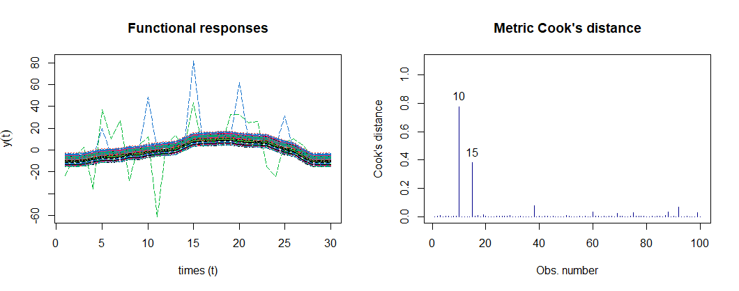
The 10th response has spikes at periodic intervals of 5 up to the 25th time point, while the 15th response has a very large variation. The distance metric based on DFT takes both the phase and amplitude variations into account. Hence, we expect it to be able to detect the two unusual observations. In Figure 5, the metric Cook’s distance accurately detects the 10th and 15th observations as influential observations.

3.4 Effects of trimming influential observations

The second part of the experimental studies is to demonstrate the impact of influential observations on the bias associated with the estimation of $\beta$ in small and large samples. The bias is reported as the angle $\theta$ between the true $\beta$ and the estimate $\hat{\beta}$ based on the samples with and without the outliers. We define $\theta$ as

$$\theta=arccosine\left(\hat{\beta}^{\top}\beta/\lVert\hat{\beta}\rVert_{2}\lVert\beta\rVert_{2}\right).$$ (9)

For each example, we report the bias associated with the samples with and without influential observations. In very large samples, the effect of influential observations diminishes drastically while in very small samples the impact is inflated. Therefore, we consider $n=\{50,100\}$ for our small and large samples. We classify an observation as influential if its metric Cook’s distance exceeds $\cfrac{4}{n-p-1}$. The results of the simulation studies are given in Tables 1-4.

Table 1: Mean (standard deviation) of $\theta$ based on 500 random replicates for Examples 1. * denotes samples without influential observations.

Example	n	p	OLS	OLS*	SIR	SIR*
I	50	5	0.2787	0.1417	1.6198	1.6033
			(0.0057)	(0.0028)	(0.0588)	(0.0609)
		10	0.455	0.2369	1.5926	1.5775
			(0.0064)	(0.0031)	(0.0512)	(0.0545)
	100	5	0.1534	0.0939	1.5992	1.5698
			(0.003)	(0.0017)	(0.0631)	(0.064)
		10	0.2451	0.1459	1.6152	1.6154
			(0.0036)	(0.0019)	(0.0589)	(0.0604)

In Table 1, we see that under the classical multiple linear regression model in Example 1, OLS yields a better estimate of $\beta$ compared to SIR. This is not surprising as the OLS estimator is the best linear unbiased estimator in this setting. However, the accuracy of OLS is severely impacted by the presence of influential observations. SIR on the other hand, is more robust to the influential observations. In contrast, in example 2, both the reduced-rank OLS (RR-OLS) estimator and SIR appear to be robust to the presence of influential observations.

For the distributional response model in example 3, we explore the effects of influential observations on the surrogate-assisted and Fréchet OLS and SIR. Here, all the methods show improvement without influential observations with the exception of sa-SIR. The fOLS and sa-OLS methods appear to be more sensitive compared to the SIR-based methods.

Table 2: Mean (standard deviation) of $\theta$ based on 500 random replicates for Examples 2. * denotes samples without influential observations.

Example	n	p	RR-OLS	RR-OLS*	SIR	SIR*
II	50	5	2.6000	2.6487	1.5349	1.5050
			(0.0198)	(0.0154)	(0.0457)	(0.0463)
		10	2.3931	2.3970	1.5517	1.5335
			(0.0143)	(0.0137)	(0.0323)	(0.0334)
	100	5	2.7897	2.7956	1.5380	1.4710
			(0.0151)	(0.0134)	(0.0552)	(0.0553)
		10	2.6344	2.6278	1.5365	1.5818
			(0.0102)	(0.0087)	(0.0462)	(0.0463)

Table 3: Mean (standard deviation) of $\theta$ based on 500 random replicates for Examples 3. * denotes samples without influential observations.

Example	n	p	fOLS	fOLS*	sa-OLS	sa-OLS*	fSIR	fSIR*	sa-SIR	sa-SIR*
III	50	5	1.3342	1.1153	1.3052	1.1374	1.3112	1.2969	1.3208	1.3216
			(0.0163)	(0.0206)	(0.0158)	(0.0208)	(0.0201)	(0.0202)	(0.0205)	(0.0196)
		10	1.4038	1.2937	1.3944	1.2883	1.4228	1.4164	1.4218	1.4379
			(0.012)	(0.0163)	(0.0116)	(0.0152)	(0.0147)	(0.0153)	(0.0145)	(0.0146)
	100	5	1.3330	1.1362	1.3082	1.1091	1.3308	1.3254	1.3218	1.3266
			(0.0162)	(0.0204)	(0.0154)	(0.0199)	(0.0194)	(0.0203)	(0.0197)	(0.0195)
		10	1.4022	1.2402	1.3986	1.2199	1.4147	1.4104	1.4215	1.4047
			(0.0126)	(0.0163)	(0.0117)	(0.0161)	(0.0147)	(0.0155)	(0.0149)	(0.0148)

Lastly, for the functional responses in example 4, we again observe that influential observations can have severe impacts on the accuracy of sa-OLS. Overall, OLS and its extensions to different response classes are more responsive to the presence of influential observations in the data than the SIR-based methods. This is not a surprising outcome as OLS is known to be easily impacted by extreme observations.

Table 4: Mean (standard deviation) of $\theta$ based on 500 random replicates for Examples 4. * denotes samples without influential observations.

Example	n	p	sa-OLS	sa-OLS*	sa-SIR	sa-SIR*
IV	50	5	0.6949	0.1851	0.2124	0.2003
			(0.0234)	(0.0068)	(0.0064)	(0.0061)
		10	1.0714	0.4124	0.4125	0.4285
			(0.0213)	(0.0169)	(0.0109)	(0.0130)
	100	5	0.3945	0.0994	0.1238	0.1077
			(0.0206)	(0.0021)	(0.0023)	(0.0020)
		10	0.6648	0.1603	0.1972	0.1781
			(0.0241)	(0.0027)	(0.0028)	(0.0026)

4 Real data analysis

So far, we have seen how the metric Cook’s distance performs with synthetic data. We now turn our attention to real data analysis. Our data is the same data used in Soale and Dong, (2023), where a detailed description of the data can be found. The responses are the daily COVID-19 transmission rate per 100, 000 persons in the United States. The transmission rate is reported as the change in the 7-day moving average of newly reported COVID cases for a given county. The timeline for our data is between 08/1/2021 and 02/21/2022. The data can be found at the Centers for Disease Control and Prevention (CDC) website (CDC, (2023)). Some counties reported transmission rates for only a few days within the study period. Therefore, we restricted our analysis sample to counties with at least 50 reported rates. We further eliminated the counties whose transmission distributions we could not smooth to obtain their probability densities, resulting in a final analysis sample of 2126 counties.

The predictors are county-level demographic information from the 2020 American Community Survey (ACS)(US Census Bureau, (2022)). The predictors include % Non-Hispanic Blacks, % Hispanics, % adults aged 65+, % adults with no high school education, % adults with a high school diploma, % population in poverty, % unemployed, % renter-occupied homes, % population on public assistance programs, and median household income. This data is also publicly available. Like Soale and Dong, (2023), we consider the responses as functional and distributional objects.

4.1 Transmissions over time as functional response

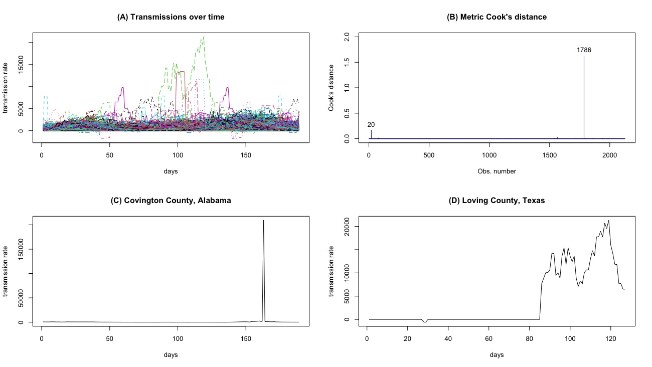
We consider the trajectories of the transmission rates over time for each county as a response. The descriptive plot and the metric Cook’s distances are given in Figure 8. We left out Covington County, Alabama which had a transmission rate of 20000/100k for one of the days to allow for better visualization in exhibit (A). The metric Cook’s distances show two influential observations, which are indicated in exhibits (C) and (D).

Figure 6: Metric Cook’s distances for regression of functional response COVID transmission rates. The time series of observation 20 (Covington, Alabama) and 1786 (Loving, Texas) are illustrated.

Since the structural dimension is unknown, we examined the scree plot of the eigenvalues of the candidate matrices for sa-OLS and sa-SIR and determined it to be 1. The basis estimates of the central space based on sa-OLS and sa-SIR with and without the influential observations are given in Table 5.

Table 5: Bases estimates with and without outliers. * denotes the sample without outliers. Bold indicates a large change in estimate after removing influential observations.

	sa-OLS	sa-OLS*	sa-SIR	sa-SIR*
% Non-Hispanic Blacks	0.3039	0.2288	0.1995	0.2358
% Hispanics	-0.0749	-0.6650	-0.6479	-0.6164
% Adults 65+	-0.8568	-0.3857	-0.3199	-0.2716
% No high school diploma	-0.1834	0.2184	0.2802	0.2756
% High school diploma	-0.0301	-0.0595	0.1093	0.1049
% Living in poverty	0.4125	-0.4274	-0.4606	-0.4794
% Unemployed	-0.2644	-0.0501	0.0272	0.0163
% Renter-occupied homes	-1.0045	-0.0378	0.0613	0.0769
% On public assistance	0.0382	-0.1822	-0.1126	-0.1179
Median Household income	0.1316	-0.1224	0.1019	0.1127

The % of Adults who are 65 and older and the % of renter-occupied homes appear to be the most important factors deriving the transmission rates based on the sa-OLS estimates for the full sample. However, after eliminating the two influential observations, we see that % Hispanic is the dominant factor. The % of people living in poverty and % of older adults also have a moderate effect on the trajectory of transmission rates. The estimate for sa-SIR is similar to the sa-OLS estimates when the two influential counties were removed. Again, sa-SIR appears to be somewhat robust to the presence of influential observations.

To illustrate the impact of the two influential functions we fit a functional-on-scalar regression using the original responses and the sufficient predictor $\hat{\beta}^{\top}{\bf X}$. The responses were first smoothed using 10 B-spline functions. The estimated average transmission rates are given in Figure 7.

Figure 7: Predicted transmission rates based on the sufficient predictors of sa-OLS and sa-SIR. * denotes the estimates without outliers.

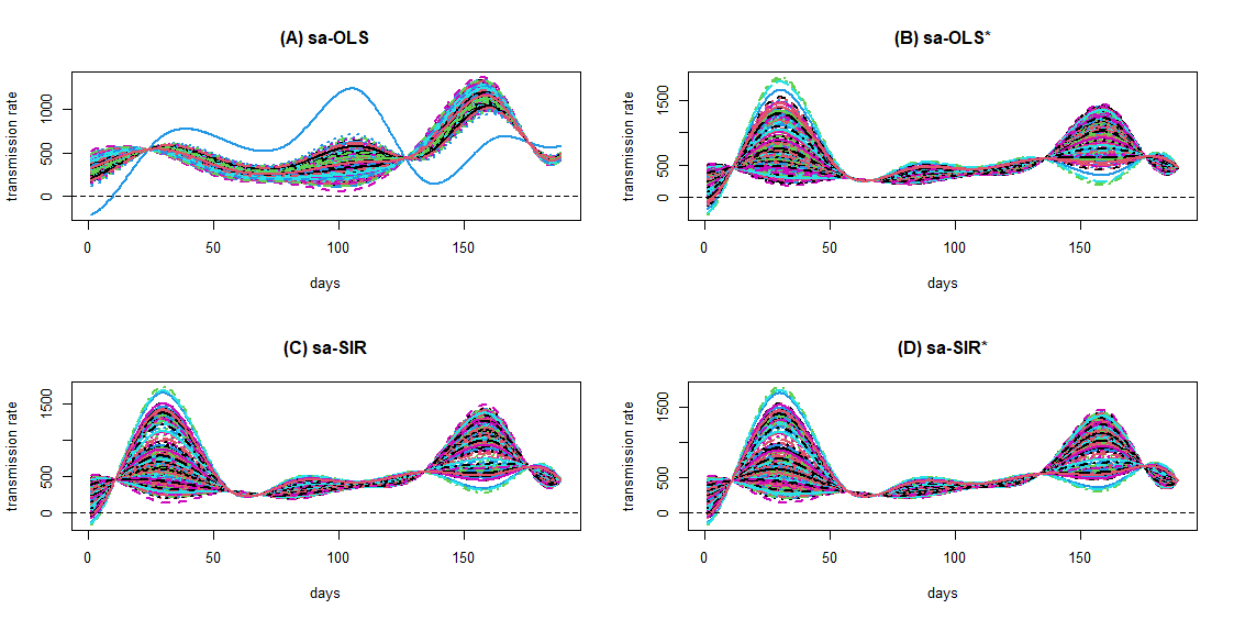
The estimate for Loving County, Texas based on the sa-OLS predictor indicated in blue in exhibit (A). For exhibit (A), nearly 15% of the total variation in transmission rates over the study period is due to phase variation. However, when we take out the two influential observations, only about 4% of the total variation is due to phase variation. The latter is similar to the results based on sa-SIR with and without outliers. The two peaks in exhibits (B), (C), and (D), are consistent with the CDC’s announcement of an additional $300 million in September of 2021 and the Biden Administration’s $2.1 billion investment in public health departments across the country to increase testing. The peak on the right coincides with the emergence of the Omicron variant. Thus, we can conclude that eliminating the outliers yields a better result.

4.2 Transmission rate distribution as response

If we are merely, interested in the distributions of the transmission rate for counties in the study period, we can simply treat the distribution of the rates as the response. We start by smoothing the histograms of the transmission rates for each county to obtain probability density functions using the Fréchet package in R. The distributional responses are independent of the reporting dates.

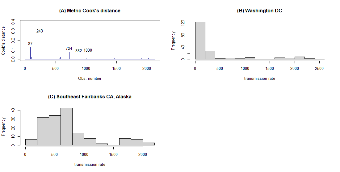
We applied the surrogate-assisted and Fréchet OLS and SIR used for example 3 in Section 3 to check for influential observations. Both fSIR and sa-SIR were implemented using 10 slices. The metric Cook’s distances are given in Figure 8. Based on the metric Cook’s distance, there are five potential influential observations, with the 87th and 243rd as the most influential. The 87th observation is determined to be Washington DC and the 243rd, Southeast Fairbanks Census Area in the State of Alaska. Their distributions are shown in the histograms in exhibits (B) and (C) in Figure 8. Both distributions are heavily right-skewed and transmission rates for Southeast Fairbanks appear to come from two clusters.

Next, we investigated the effect of the influential observations on the estimated basis directions. The estimated bases are provided in Table 6. The influential observations appear to have little effect on the SIR-based methods. However, they have quite an influence on the fOLS and sa-OLS estimates. For fOLS, we see the loadings for % Non-Hispanic Blacks and % unemployed almost double while that of median household income is almost half after removing the influential observations. Similarly, almost all the loadings for sa-OLS changed in magnitude and sometimes direction when the influential observations were removed.

Figure 8: Metric Cook’s distances for regression of distributional response COVID transmission rates. The distributions of observation 87 (Washington DC) and 243 (SE Fairbanks, Alaska) are illustrated.

Table 6: Bases estimates with and without outliers. * denotes the sample without outliers. Bold indicates a large change in estimate after removing influential observations.

	fOLS	fOLS*	sa-OLS	sa-OLS*	fSIR	fSIR*	sa-SIR	sa-SIR*
% Non-Hispanic Blacks	-0.1733	-0.3036	0.0300	-0.1697	0.6921	-0.6955	-0.6863	-0.6880
% Hispanics	-0.1320	-0.1193	0.0561	0.2565	0.3155	-0.3143	-0.2427	-0.2373
% Adults 65+	0.2123	0.2402	-0.2281	-0.0150	-0.1096	0.1156	0.1413	0.1454
% No high school diploma	-0.7250	-0.7003	-0.5639	-0.8059	0.1918	-0.1838	-0.2148	-0.2153
% High school diploma	0.2162	0.2490	0.3863	0.9098	0.0120	-0.0166	-0.0684	-0.0742
% Living in poverty	0.4939	0.3259	0.3332	0.3223	0.2773	-0.2918	-0.3060	-0.3107
% Unemployed	-0.1456	-0.2384	0.3812	0.1102	0.0639	-0.0683	-0.0929	-0.0987
% Renter-occupied homes	-0.0873	-0.0099	-0.0621	-0.1105	-0.1619	0.1635	0.1463	0.1425
% On public assistance	0.1447	0.1570	0.0402	0.1039	-0.1266	0.1231	0.1088	0.1081
Median Household income	0.6304	0.3332	1.0515	0.6541	-0.0180	-0.0046	-0.0697	-0.0902

5 Conclusions

In this paper, we presented a general framework for detecting influential observations for regression with metric-valued responses on Euclidean predictors. As demonstrated in Example 2, even in Euclidean space, the proposed metric Cook’s distance can be very useful in regression with rank-reduced vector responses. We also demonstrated that influential observations can have a significant impact on the estimate of the central space even in the emerging random object regression.

A future study that explores the effects of outliers beyond the single index models and on object-on-object regression will be interesting to pursue.

Appendix

Proof of Lemma 1.

If $Y\perp\!\!\!\perp{\bf X}|\beta^{\top}{\bf X}$, then $(Y,\tilde{Y})\perp\!\!\!\perp{\bf X}|\beta^{\top}{\bf X}$ also hold, for any random copy $\tilde{Y}$ of $Y$. By Theorem 2.3 of Li(2018), we have that $\phi(Y,\tilde{Y})\perp\!\!\!\perp{\bf X}|\beta^{\top}{\bf X}$ Li, (2018). ∎

Proof of Theorem 1.

By Lemma 1, $\mathcal{S}_{S^{Y}|{\bf X}}\subseteq{\mathcal{S}}_{Y|{\bf X}}$. The ordinary least squares estimator $\bm{\Sigma}^{-1}\bm{\Sigma}_{XS^{Y}}\in\mathcal{S}_{\operatorname{E}(S^{Y}|{\bf X})}\subseteq\mathcal{S}_{S^{Y}|{\bf X}}$ by Theorem 8.3 of Li, (2018), which leads to the desired results. ∎

References

- Agrawal et al., (1993) Agrawal, R., Faloutsos, C., and Swami, A. (1993). Efficient similarity search in sequence databases. In Foundations of Data Organization and Algorithms: 4th International Conference, FODO’93 Chicago, Illinois, USA, October 13–15, 1993 Proceedings 4, pages 69–84. Springer.
- CDC, (2023) CDC (2023). United States COVID-19 County Level of Community Transmission Historical Changes. [Online; accessed 13-March-2023].
- Chen et al., (2022) Chen, F., Shi, L., Zhu, L., and Zhu, L. (2022). A method of local influence analysis in sufficient dimension reduction. Statistica Sinica, 32(2).
- Cook, (1977) Cook, R. D. (1977). Detection of influential observation in linear regression. Technometrics, 19(1):15–18.
- Cook, (1996) Cook, R. D. (1996). Graphics for regressions with a binary response. Journal of the American Statistical Association, 91(435):983–992.
- Dong and Wu, (2022) Dong, Y. and Wu, Y. (2022). Fréchet kernel sliced inverse regression. Journal of Multivariate Analysis, 191:105032.
- Eaton, (1986) Eaton, M. L. (1986). A characterization of spherical distributions. Journal of Multivariate Analysis, 20(2):272–276.
- Faraway, (2014) Faraway, J. J. (2014). Regression for non-euclidean data using distance matrices. Journal of Applied Statistics, 41(11):2342–2357.
- Gather et al., (2002) Gather, U., Hilker, T., and Becker, C. (2002). A note on outlier sensitivity of sliced inverse regression. Statistics: A Journal of Theoretical and Applied Statistics, 36(4):271–281.
- Kruskal, (1964) Kruskal, J. B. (1964). Multidimensional scaling by optimizing goodness of fit to a nonmetric hypothesis. Psychometrika, 29(1):1–27.
- Kruskal and Wish, (1978) Kruskal, J. B. and Wish, M. (1978). Multidimensional scaling. Number 11. Sage.
- Li, (2018) Li, B. (2018). Sufficient dimension reduction: Methods and applications with R. CRC Press.
- Li, (1991) Li, K.-C. (1991). Sliced inverse regression for dimension reduction. Journal of the American Statistical Association, 86(414):316–327.
- Li and Duan, (1989) Li, K.-C. and Duan, N. (1989). Regression analysis under link violation. The Annals of Statistics, 17(3):1009–1052.
- Petersen and Müller, (2019) Petersen, A. and Müller, H.-G. (2019). Fréchet regression for random objects with euclidean predictors.
- Prendergast, (2008) Prendergast, L. A. (2008). Trimming influential observations for improved single-index model estimated sufficient summary plots. Computational statistics & data analysis, 52(12):5319–5327.
- Soale and Dong, (2023) Soale, A.-N. and Dong, Y. (2023). Data visualization and dimension reduction for metric-valued response regression. arXiv preprint arXiv:2310.12402.
- US Census Bureau, (2022) US Census Bureau (2022). United States Census Bureau. https://www.census.gov/data.html. Accessed: 2022-10-26.
- Yin et al., (2008) Yin, X., Li, B., and Cook, R. D. (2008). Successive direction extraction for estimating the central subspace in a multiple-index regression. Journal of Multivariate Analysis, 99(8):1733–1757.
- Zhang et al., (2021) Zhang, Q., Xue, L., and Li, B. (2021). Dimension reduction and data visualization for fr’echet regression. arXiv preprint arXiv:2110.00467.