Ordinals and recursive algorithms

Abstract

Given a function $f:\mathbb{R}\to\mathbb{R}$, call a decreasing sequence $x_{1}>x_{2}>x_{3}>\cdots$ $f$-bad if $f(x_{1})>f(x_{2})>f(x_{3})>\cdots$, and call the function $f$ ordinal decreasing if there exist no infinite $f$-bad sequences. We prove the following result, which generalizes results of Erickson et al. (2022) and Bufetov et al. (2024): Given ordinal decreasing functions $f,g_{1},\ldots,g_{k},s$ that are everywhere larger than $0$, define the recursive algorithm “$M(x)$: if $x<0$ return $f(x)$, else return $g_{1}(-M(x-g_{2}(-M(x-\cdots-g_{k}(-M(x-s(x)))\cdots))))$”. Then $M(x)$ halts and is ordinal decreasing for all $x\in\mathbb{R}$.

More specifically, given an ordinal decreasing function $f$, denote by $o(f)$ the ordinal height of the root of the tree of $f$-bad sequences. Then we prove that, for $k\geq 2$, the function $M(x)$ defined by the above algorithm satisfies $o(M)\leq\varphi_{k-1}(\gamma+o(s)+1)$, where $\gamma$ is the smallest ordinal such that $\max{\{o(s),o(f),o(g_{1}),\ldots,o(g_{k})\}}<\varphi_{k-1}(\gamma)$.

Keywords: Ordinal, recursive algorithm, ordinal decreasing function, fusible number, Veblen function.

1 Introduction

Erickson, Nivasch and Xu [4, 5, 7] studied the following recursive algorithm $M$:

$$M(x)=\begin{cases}-x,&\text{if $x<0$;}\\ \frac{M(x-M(x-1))}{2},&\text{if $x\geq 0$.}\end{cases}$$ (1)

For example it can be checked that $M(1)=\frac{M(1-M(0))}{2}=\frac{1}{8}$, $M(\frac{3}{2})=\frac{1}{32}$, $M(2)=2^{-10}$, $M(\frac{5}{2})=2^{-31}$ and $M(3)=2^{-1,541,023,937}$ (see Figure 1).

Erickson, Nivasch and Xu [4, 5, 7] proved that $M$ terminates on all real inputs, although Peano Arithmetic cannot prove that $M$ terminates on all natural inputs. PA-independence was shown by proving that $\frac{1}{M(n)}$ grows as fast as $F_{\varepsilon_{0}}(n-7)$ for integers $n\geq 8$.

The motivation for algorithm $M$ lies in the set of fusible numbers. As Erickson et al. [4] showed, $M(x)$ returns the distance between $x$ and the smallest “tame fusible number” larger than $x$. However, algorithm $M$ is worth studying on its own right, since it is a simple algorithm for which its termination is not so easy to prove.

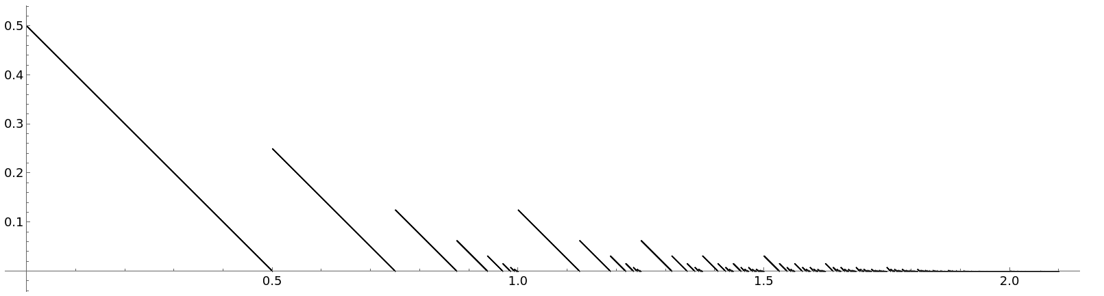
Figure 1: The graph of $M(x)$ up to $x=2.1$.

In a follow-up paper, Bufetov et al. [1] studied a generalization of fusible numbers to $n$-fusible numbers and a corresponding generalization of algorithm $M$ to the following algorithm $M_{n}$:

$$M_{n}(x)=\begin{cases}-x,&\text{if $x<0$;}\\ \frac{M_{n}(x-M_{n}(x-\cdots-M_{n}(x-1)\cdots))}{n},&\text{if $x\geq 0$;}\end{cases}$$ (2)

where $M_{n}(x-\cdots)$ repeats $n$ times. They showed that for every $n\geq 1$, $M_{n}$ terminates on all real inputs. In this paper we study the following question: Which modifications can be done to algorithm $M$ such that it will still halt on all real inputs?

We identify a large class of algorithms that halt on all real inputs. The description of the algorithms, as well as the proof that they halt on all real inputs, involve a property of real-valued functions, which we call ordinal decreasing.

1.1 Ordinal decreasing functions

Definition 1.1.

Given a function $f:D\to\mathbb{R}$ for some $D\subseteq\mathbb{R}$, we call a descending sequence $x_{1}>x_{2}>x_{3}>\cdots$ in $D$ $f$-bad if $f(x_{1})>f(x_{2})>f(x_{3})>\cdots$. We call the function $f$ ordinal decreasing there exist no infinite $f$-bad sequences. We call $f$ ordinal decreasing up to $a$ if it is ordinal decreasing in the interval $(-\infty,a]\subseteq D$.

Some examples of ordinal decreasing functions are:

1. Every nonincreasing function.

2. A function $f$ in the domain $[0,1)$ that is divided into a sequence of intervals $\{I_{n}\}$ where $I_{n}=[1-2^{-n},1-2^{-n+1})$ and where $f$ is decreasing in each interval (see Figure 2, left).

3. A function $f$ in the domain $(0,1]$ that is divided into a sequence of intervals $\{I_{n}\}$ where $I_{n}=(2^{-(n+1)},2^{-n}]$, such that $f$ is decreasing in each $I_{n}$ but such that for each $n$ there exist only finitely many $n<m$ such that $2^{-m}>\lim_{x\to(2^{-n})^{+}}(f(x))$ (see Figure 2, right).

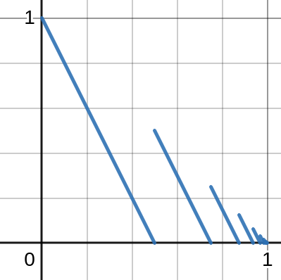
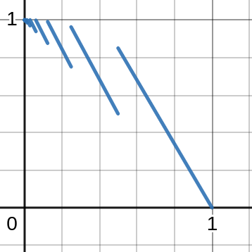
Figure 2: Examples of ordinal decreasing functions.

Let $f$ be an ordinal decreasing function. Borrowing a notion from well partial orders (see Section 2.4 below), we define the tree of $f$-bad sequences $T_{f}$ as the (possibly infinite) tree that contains a vertex $v_{f}(\overline{x})$ for each $f$-bad sequence $\overline{x}=\langle x_{1}>\cdots>x_{n}\rangle$, and contains an edge connecting each $v_{f}(\langle x_{1}>\cdots>x_{n}\rangle)$, $n\geq 1$ to its parent $v_{f}(\langle x_{1}>\cdots>x_{n-1}\rangle)$. The root of the tree is $v_{f}(\langle\rangle)$, corresponding to the empty sequence.

Since $T_{f}$ contains no infinite path, there exists a unique way to assign to each vertex $v\in T_{f}$ an ordinal height $o(v)$, such that $o(v)=\lim_{\text{$w$ child of $v$}}(o(w)+1)$ for all $v\in T_{f}$. We define the ordinal type $o(f)$ of the function $f$ to be the ordinal height of the root of $T_{f}$, meaning $o(f)=o(v_{f}(\langle\rangle))$.

Given $x\in D$, we define $o_{f}$ to be the function from the reals to the ordinals recursively given by $o_{f}(x)=\lim_{x^{\prime}<x,f(x^{\prime})<f(x)}(o_{f}(x^{\prime})+1)$. Then it is easy to verify that $o(f)=\lim_{x\in\mathbb{R}}(o_{f}(x)+1)$.

Given an interval $D\subset\mathbb{R}$, let $o(f|_{D})$ denote the ordinal type of the restriction of $f$ to $D$.

1.2 Our results

Now we can state the main results of our paper.

Theorem 1.2.

Consider the recursive algorithm:

$$M(x)=\begin{cases}f(x)&\text{if $x<0$;}\\ g_{1}(-M(x-g_{2}(-M(x-\cdots-g_{k}(-M(x-s(x)))\cdots))))&\text{if $x\geq 0$;}\end{cases}$$ (3)

where the functions $s(x)$, $f(x)$ and $g_{i}(x)$ for all $i$ are all ordinal decreasing and larger than 0 for every $x$ in the appropriate ranges: $(-\infty,0)$ for $f,g_{i},h$, and $[0,\infty)$ for $s$.

Then $M(x)$ halts and is ordinal decreasing for all $x\in\mathbb{R}$.

Note that Theorem 1.2 covers the cases mentioned above, by taking $k=n$, $g_{1}(x)=-\frac{x}{n}$, $g_{i}(x)=-x$ for $2\leq i\leq n$ and $s(x)=1$.

We also prove the following upper bounds on $o(M)$ in terms of $k$ and $o(f),o(s),o(g_{1}),\ldots,o(g_{k})$.

Theorem 1.3.

Let $M$ be the function computed by the algorithm of Theorem 1.2. If $k=1$, then let $\gamma$ be minimal such that $\max{\{o(f),o(s),o(g_{1})\}}<\omega^{\omega^{\gamma}}$. Then $o(M)\leq\omega^{\omega^{\gamma+1}(o(s)+1)}$. For $k\geq 2$, let $\gamma$ be minimal such that $\max{\{o(f),o(s),o(g_{1}),\ldots,o(g_{k})\}}<\varphi_{k-1}(\gamma)$. Then $o(M)\leq\varphi_{k-1}(\gamma+o(s)+1)$.

By comparison, the specific function $M$ of Erickson et al. [5] satisfies $o(M)=\varphi_{1}(0)=\varepsilon_{0}$, and the generalization of Bufetov et al. [1] satisfies $o(M)=\varphi_{n-1}(0)$.

2 Background

2.1 Real induction

In this paper we will use the following result, which is called real induction (see Clark [2] for a survey).

Lemma 2.1.

Let $S\subset\mathbb{R}$ be a set that satisfies:

(R1) There exists $a\in\mathbb{R}$ such that $(-\infty,a)\subset S$.

(R2) For all $x\in\mathbb{R}$, if $(-\infty,x)\subset S$, then $x\in S$.

(R3) For all $x\in S$, there exists $y>x$ such that $(x,y)\subset S$.

Then $S=\mathbb{R}$.

Proof.

Suppose $S\neq\mathbb{R}$. Let $a=\inf(\mathbb{R}\setminus S)$. By (R1) $a\neq-\infty$. Therefore by (R2), $a\in S$. Therefore (R3) yields a contradiction. ∎

It is worth noting for our purposes that since Peano Arithmetic is built upon the natural numbers, we cannot use real induction within Peano Arithmetic, but must rely on Second Order Arithmetic.

2.2 Veblen functions

The finite Veblen functions $\varphi_{n}$, $n\in\mathbb{N}$ are a sequence of functions from ordinals to ordinals, defined by starting with $\varphi_{0}(\alpha)=\omega^{\alpha}$, and for each $n\in\mathbb{N}$, letting

$$\varphi_{n+1}(0) =\lim_{k\in\mathbb{N}}\varphi_{n}^{(k)}(0);$$

$$\varphi_{n+1}(\alpha+1) =\lim_{k\in\mathbb{N}}\varphi_{n}^{(k)}(\varphi_{n+1}(\alpha)+1);$$

$$\varphi_{n+1}(\alpha) =\lim_{\beta<\alpha}\varphi_{n+1}(\beta),\qquad\text{$\alpha$ limit}.$$

Here $f^{(k)}=\underbrace{f\circ f\circ\cdots\circ f}$ denotes $k$-fold application of $f$. Ordinals of the form $\varphi_{1}(\alpha)$ are called epsilon numbers, and are denoted $\varepsilon_{\alpha}=\varphi_{1}(\alpha)$.

2.3 Natural sum and product of ordinals

Given ordinals $\alpha,\beta$ with Cantor Normal Forms

$$\alpha =\omega^{\alpha_{1}}+\ldots+\omega^{\alpha_{n}},\qquad\text{ with $\alpha_{1}\geq\ldots\geq\alpha_{n}$},$$

$$\beta =\omega^{\beta_{1}}+\ldots+\omega^{\beta_{m}},\qquad\text{ with $\beta_{1}\geq\ldots\geq\beta_{m}$};$$

their natural sum $\alpha\oplus\beta$ is given by $\omega^{\gamma_{1}}+\ldots+\omega^{\gamma_{n+m}}$, where $\gamma_{1},\ldots,\gamma_{n+m}$ are $\alpha_{1},\ldots,\alpha_{n},\beta_{1},\ldots,\beta_{m}$ sorted in nonincreasing order. The natural product of $\alpha,\beta$ is given by

$$\alpha\otimes\beta=\mathop{\bigoplus\limits_{1\leq i\leq n}}\limits_{1\leq j\leq m}\omega^{\alpha_{i}\oplus\beta_{j}}.$$

(See e.g. de Jongh and Parikh [3].)

The natural sum and natural product operations are commutative and associative, and natural product distributes over natural sum. These operations are also monotonic, in the sense that if $\alpha<\beta$ then $\alpha\oplus\gamma<\beta\oplus\gamma$, if $\alpha\leq\beta$ then $\alpha\otimes\gamma\leq\beta\otimes\gamma$, and if $\alpha<\beta$ and $\gamma>0$ then $\alpha\otimes\gamma<\beta\otimes\gamma$. Furthermore, $\alpha+\beta\leq\alpha\oplus\beta$ and $\alpha\beta\leq\alpha\otimes\beta$.

Recall that if $\alpha=\omega^{\alpha_{1}}+\cdots+\omega^{\alpha_{k}}$ is in CNF, then $\alpha\omega=\lim_{n\in\mathbb{N}}\alpha n=\omega^{\alpha_{1}+1}$, and $\alpha^{\omega}=\lim_{n\in\mathbb{N}}\alpha^{n}=\omega^{\alpha_{1}\omega}$. Then the following properties are readily checked:

• $\underbrace{\alpha\oplus\cdots\oplus\alpha}_{n}=\alpha\otimes n,\qquad n\in\mathbb{N}$;

• $\lim_{n\in\mathbb{N}}\alpha\oplus n=\alpha+\omega$ (not $\alpha\oplus\omega$!);

• if $\alpha$ and $\beta$ are limit ordinals, then $\alpha\oplus\beta=\lim_{\alpha^{\prime}<\alpha,\beta^{\prime}<\beta}(\alpha^{\prime}\oplus\beta^{\prime})$;

• $\lim_{n\in\mathbb{N}}\alpha\otimes n=\alpha\omega$ (not $\alpha\otimes\omega$!);

• if both $\alpha<\omega^{\gamma}$ and $\beta<\omega^{\gamma}$ then $\alpha\oplus\beta<\omega^{\gamma}$;

• if both $\alpha<\omega^{\omega^{\gamma}}$ and $\beta<\omega^{\omega^{\gamma}}$ then $\alpha\otimes\beta<\omega^{\omega^{\gamma}}$.

Define the repeated natural product by transfinite induction, by letting $\alpha^{[0]}=1$, $\alpha^{[\beta+1]}=\alpha^{[\beta]}\otimes\alpha$, and $\alpha^{[\beta]}=\lim_{\gamma<\beta}\alpha^{[\gamma]}$ for limit $\beta$. It can be checked that

$$\alpha^{[\omega]}=\lim_{n\in\mathbb{N}}\alpha^{[n]}=\lim_{n\in\mathbb{N}}(\alpha\otimes\cdots\otimes\alpha)=\alpha^{\omega}.$$

In general, for limit $\beta$ we have $\alpha^{[\beta]}=\alpha^{\beta}$, as can be shown by ordinal induction on $\beta$. It can also be shown by ordinal induction on $\beta$ that $(\omega^{\omega^{\alpha}})^{[\beta]}=(\omega^{\omega^{\alpha}})^{\beta}$.

2.4 Well partial orders

Given a set $A$ partially ordered by $\preceq$, a bad sequence is a sequence $a_{1},a_{2},a_{3}\ldots$ of elements of $A$ such that there exist no indices $i<j$ for which $a_{i}\preceq a_{j}$. Then $\preceq$ is said to be a well partial order (WPO) if there exist no infinite bad sequences of elements of $A$. The ordinal type of $A$, denoted $o(A)$, is the ordinal height of the root of the tree of bad sequences of $A$. It also equals the maximal order type of a linear order $\leq$ extending $\preceq$ (de Jongh and Parikh [3]).

Given WPOs $A$ and $B$, their disjoint union $A\sqcup B$ can be well partially ordered by letting $x\preceq y$ if and only if $x,y\in A$ and $x\preceq_{A}y$ or $x,y\in B$ and $x\preceq_{B}y$. Then $o(A\sqcup B)=o(A)\oplus o(B)$ [3]. Also, their Cartesian product $A\times B$ can be well partially ordered by letting $(a,b)\preceq(a^{\prime},b^{\prime})$ if and only if $a\preceq_{A}a^{\prime}$ and $b\preceq_{B}b^{\prime}$. Then $o(A\times B)=o(A)\otimes o(B)$ [3].

3 Proof of Theorem 1

We start by proving some properties of ordinal decreasing functions.

Lemma 3.1.

Suppose $f(x)$ is ordinal decreasing up to $y$. Then for every infinite decreasing sequence $\{x_{n}\}$ with $x_{0}<y$ there is an infinite subsequence $\{x^{\prime}_{n}\}$ for which $\{f(x^{\prime}_{n})\}$ is nondecreasing.

Proof.

By the infinite Ramsey’s theorem. Define an infinite complete graph in which there is a vertex for each $x_{i}$ and color each edge $\{x_{i},x_{j}\},i<j$ red if $f(x_{i})>f(x_{j})$ and green otherwise.

Since $f(x)$ is ordinal decreasing up to $y$ our graph cannot contain a monochromatic red infinite complete subgraph. Therefore there exists a monochromatic green infinite subgraph, and thus the original sequence contains an infinite nondecreasing subsequence (comprised of all the vertices in the subgraph). ∎

Lemma 3.2.

Suppose $g(x)$ is ordinal decreasing up to $y$ and $f(x)$ is ordinal decreasing up to $\sup_{x<y}(-g(x))$. Then $f(-g(x))$ is ordinal decreasing up to $y$.

Proof.

Consider an infinite decreasing sequence $\{x_{n}\}$ with $x_{0}<y$. By Lemma 3.1, there exists a nondecreasing subsequence of $\{g(x_{n})\}$. If this subsequence is not strictly increasing, there exists $i<j$ such that $g(x_{i})=g(x_{j})$, and so is $f(-g(x_{i}))=f(-g(x_{j}))$. Otherwise we have a strictly decreasing sequence of $-g(x)$, and since $f(x)$ is ordinal decreasing up to $\sup_{x<y}(-g(x))$, we can find $f(-g(x_{j}))\geq f(-g(x_{i}))$, and we are done. ∎

Lemma 3.3.

Suppose $f(x)$ and $g(x)$ are ordinal decreasing up to $y$. Then $f(x)+g(x)$ is ordinal decreasing up to $y$.

Proof.

By Lemma 3.1, for every strictly decreasing sequence $\{x_{n}\}$ with $x^{\prime}_{0}<y$ we can find a subsequence $\{x^{\prime}_{n}\}$ such that $\{f(x^{\prime}_{n})\}$ is nondecreasing. For that subsequence we can find by definition $i<j$ such that $g(x_{j})\geq g(x_{i})$. Hence, $f(x^{\prime}_{j})+g(x^{\prime}_{j})\geq f(x^{\prime}_{i})+g(x^{\prime}_{i})$ as desired. ∎

(In this paper we only use Lemma 3.3 for the special case $g(x)=-x$.)

Lemma 3.4.

Let $\beta>0$, and suppose $f(x)$ is ordinal decreasing up to $y+\beta$ and larger than $0$. Then there exists an $0<\varepsilon<\beta$ such that $x-f(x)<y$ for every $y<x<y+\varepsilon$.

Proof.

Suppose for a contradiction that for every $0<\varepsilon<\beta$ we have a counterexample $x-f(x)\geq y$ with $y<x<y+\varepsilon$. Then, we have an infinite sequence $\{x_{n}\}$ of such counterexamples with $\lim(x_{n})=y$, but because $0<f(x_{n})\leq x_{n}-y$ there exists an infinite subsequence $\{x^{\prime}_{n}\}$ for which $f(x^{\prime}_{n})$ is decreasing, in contradiction to $f(x)$ being ordinal decreasing up to $y+\beta$. ∎

We are ready to prove our main result.

Proof of Theorem 1.2.

Consider the recursive algorithm

$$M(x)=\begin{cases}f(x),&\text{if $x<0$}\\ g_{1}(-M(x-g_{2}(-M(x-\cdots-g_{k}(-M(x-s(x)))\cdots))))&\text{if $x\geq 0$}\end{cases}$$ (4)

where $s(x)$, $f(x)$ and $g_{i}(x)$ for all $i$ are all ordinal decreasing and larger than 0 for every $x$ in the appropriate ranges: $(-\infty,0)$ for $f,g_{i},h$, and $[0,\infty)$ for $s$.

We claim that $M(x)$ halts and is ordinal decreasing for every $x$. We will prove this by real induction (Lemma 2.1).

Assuming otherwise, let

$$S=\{x\mid\text{$M$ is defined and ordinal decreasing up to $x$}\}.$$

Since for $x<0$ $M(x)$ is defined by $M(x)=f(x)$, we have $(-\infty,0)\in S$. Hence, S satisfies property (R1).

Next, suppose that $(-\infty,y)\in S$. Then note that $M(y)$ is defined, since for every $i$ $M(y-g_{i}(-M(y-\cdots-g_{k}(-M(y-s(y)))\cdots)))$ is defined by induction, since functions $g_{i}$ and $s$ have output larger than $0$. Hence, $M(x)$ is ordinal decreasing up to $y$ itself. Hence $y\in S$ as well, so $S$ satisfies property (R2).

Finally suppose $y\in S$. We will show that $(y,y+\varepsilon)\subseteq S$ for some $\varepsilon>0$, meaning $S$ satisfies property (R3).

In order to do that, we will show by induction on $i=k,\ldots,1$ that $M_{i}(x)=g_{i}(-M(x-\cdots-g_{k}(-M(x-s(x)))\cdots))$ is defined and ordinal decreasing up to $y+\varepsilon_{i}$ for some $\varepsilon_{i}>0$. Let us start with the base case $i=k$. In this case $M_{k}(x)=g_{k}(-M(x-s(x)))$. By Lemma 3.3, $-x+s(x)$ is an ordinal decreasing function in $[0,\infty)$, hence by Lemma 3.4 on $s(x)$, there is an $\varepsilon_{k}$ such that $x-s(x)<y$ for every $y<x<y+\varepsilon_{k}$. Hence, by assumption and Lemma 3.2, $M(-(-x+s(x)))=M(x-s(x))$ is ordinal decreasing and defined up to $y+\varepsilon_{k}$ and so is $g_{k}(-M(x-s(x)))$, as desired. For the induction step, suppose $M_{i}(x)$ is ordinal decreasing and defined up to $y+\varepsilon_{i}$. By Lemma 3.3, $-x+M_{i}(x)$ is ordinal decreasing and defined up to $y+\varepsilon_{i}$. Furthermore, by Lemma 3.4 there exists some $\varepsilon_{i-1}$ such that $x-M_{i}(x)<y$ for every $y<x<y+\varepsilon_{i-1}$. Hence, by assumption and Lemma 3.2 $M(x-M_{i}(x))$ is defined and ordinal decreasing up to $y+\varepsilon_{i-1}$. Hence, so is $M_{i-1}=g_{i-1}(-M(x-M_{i}(x)))$. Hence by Lemma 2.1 we have $S=\mathbb{R}$. ∎

4 Proof of Theorem 1.3

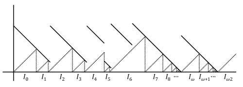
Figure 3: An ordinal decreasing function (solid line) induces a partition of the $x$-axis into a transfinite number of intervals (dotted lines).

Let $f:D\to\mathbb{R}$ be an ordinal decreasing function that is positive in some interval $D=[x_{1},x_{2})$, $x_{1}\neq-\infty$. By Lemma 3.4, the function $f$ induces a partition of $D$ into maximal intervals as follows. Define the endpoints $p_{\alpha}$ by

$$p_{0} =x_{1};$$

$$p_{\alpha+1} =\max{\{y\leq x_{2}:x-f(x)<p_{\alpha}\text{ for all $x<y$}\}};$$

$$p_{\alpha} =\lim_{\beta<\alpha}p_{\beta},\qquad\text{$\alpha$ limit.}$$

Then define the intervals $I_{\alpha}=[p_{\alpha},p_{\alpha+1})$ for ordinals $\alpha$. These intervals form a partition of $D$. Figure 3 shows how the intervals $I_{\alpha}$ can be computed graphically: Starting at $x_{1}$ on the $x$-axis, we move up-right in a straight line with slope $1$, until we encounter the graph of $f$ or pass above the graph. At that point, we descend to the $x$-axis, mark a new endpoint $p_{\alpha}$, and start this process again.

Lemma 4.1.

The ordinal number of intervals $I_{\alpha}$ into which $D$ is partitioned is at most $\omega\cdot(o(f|_{D})+1)$.

Proof.

Recall that $f$ is positive for all $x\in D$. Call $x\in D$ a near-root of $f$ if there exists an infinite increasing sequence $y_{1},y_{2},y_{3},\ldots\in D$ such that $\lim_{n\to\infty}y_{n}=x$ and $\lim_{n\to\infty}f(y_{n})=0$. Let $L_{s}\subset\mathbb{R}$ be the set of near-roots of $f$. The set $L_{f}$ is well-ordered in $\mathbb{R}$, since from an infinite decreasing sequence of near-roots we could construct an infinite $f$-bad sequence. More precisely, denoting the ordinal type of $L_{f}$ by $o(L_{f})$, we have $o(L_{f})\leq o(f)$.

Call a near-root $z\in L_{f}$ limit if there exist near-roots $z_{1},z_{2},z_{3},\ldots\in L_{f}$ that converge to $z$; otherwise call $z$ non-limit.

Observation 4.2.

Let $z\in D$. Then there exists an infinite sequence of $\omega$ consecutive intervals $I_{\alpha},I_{\alpha+1},I_{\alpha+2},\ldots$ that converge to $z$ if and only if $z$ is a non-limit near-root of $s$.

The claim follows. ∎

Lemma 4.3.

Let $J\subseteq\mathbb{R}$ be an interval, and let $J_{1}$, $J_{2}$ be a partition of $J$ into two intervals, with $J_{1}$ left of $J_{2}$. Then $o(f|_{J})\leq o(f|_{J_{1}})+o(f|_{J_{2}})$.

Proof.

Every $f$-bad sequence in $J$ can be partitioned into an $f$-bad sequence in $J_{2}$ followed by an $f$-bad sequence in $J_{1}$ (though the converse is not necessarily true). Hence, the tree of $f$-bad sequences $T_{(f|_{J})}$ is a subtree of the tree formed by attaching a copy of $T_{(f|_{J_{1}})}$ to each leaf of $T_{(f|_{J_{2}})}$. The ordinal type of this latter tree is $o(f|_{J_{1}})+o(f|_{J_{2}})$, so the claim follows. ∎

Lemma 4.4.

Let $f$ be ordinal decreasing, and let $g(x)=f(x)-x$ (which is ordinal decreasing by Lemma 3.3). Then $o(g)\leq o(f)$.

Proof.

Every $g$-bad sequence is also $f$-bad, hence $T_{g}\subseteq T_{f}$. ∎

Lemma 4.5.

Suppose $g(x)$ is ordinal decreasing up to $y$ and $f(x)$ is ordinal decreasing up to $y^{\prime}=\sup_{x<y}(-g(x))$. Let $h(x)=f(-g(x))$ (which is ordinal decreasing up to $y$ by Lemma 3.2). Then $o(h|_{y})\leq o(g|_{y})\otimes o(f|_{y^{\prime}})$.

Proof.

Let $A=o(g|_{y})\otimes o(f|_{y^{\prime}})$ be WPO by the standard product order mentioned in Section 2.4. Given $x\leq y$, let $E(x)=(o_{g}(x),o_{f}(-g(x)))\in A$.

Lemma 4.6.

If $x>x^{\prime}$ and $E(x)\preceq E(x^{\prime})$ then $h(x)\leq h(x^{\prime})$. (Hence, $E$ is analogous to what Rathjen and Weiermann [6] call a quasi-embedding.)

Proof.

We have $x>x^{\prime}$ and $o_{g}(x)\leq o_{g}(x^{\prime})$. Hence, $g(x)\leq g(x^{\prime})$ (because $x>x^{\prime}$ and $g(x)>g(x^{\prime})$ would imply $o_{g}(x)>o_{g}(x^{\prime})$). If $g(x)=g(x^{\prime})$ then $h(x)=h(x^{\prime})$ and we are done. Otherwise, $g(x)<g(x^{\prime})$, so $-g(x)>-g(x^{\prime})$. We also have $o_{f}(-g(x))\leq o_{f}(-g(x^{\prime}))$. Hence, $h(x)=f(-g(x))\leq f(-g(x^{\prime}))=h(x^{\prime})$, as desired. ∎

Hence, if $x_{1}>x_{2}>\cdots>x_{n}$ is an $h$-bad sequence then $E(x_{1}),E(x_{2}),\ldots,E(x_{n})$ is a bad sequence in $A$. Therefore, $o(h|_{y})\leq o(A)=o(g|_{y})\otimes o(f|_{y^{\prime}})$. ∎

The following lemma is not actually used in this paper:

Lemma 4.7.

Suppose $f$ and $g$ are ordinal decreasing, and let $h(x)=f(x)+g(x)$ (which is ordinal decreasing by Lemma 3.3). Then $o(h)\leq o(f)\otimes o(g)$.

Proof.

The claim follows by considering the quasi-embedding $E(x)=(o_{f}(x),o_{g}(x))$. ∎

4.1 The case $k=1$

When $k=1$ the algorithm is

$$M(x)=\begin{cases}f(x),&x<0;\\ g(-M(x-s(x))),&x\geq 0.\end{cases}$$

Consider the partition of $[0,\infty)$ into intervals induced by $s$. Namely, let

$$p_{0} =0;$$

$$p_{\alpha+1} =\max{\{y:x-s(x)<p_{\alpha}\text{ for all $x<y$}\}},\qquad\text{for $\alpha\geq 1$};$$

$$p_{\alpha} =\lim_{\beta<\alpha}p_{\beta},\qquad\text{for $\alpha$ limit}.$$

Then define the intervals $I_{-1}=(-\infty,0)$ and $I_{\alpha}=[p_{\alpha},p_{\alpha+1})$ for ordinals $\alpha$.

Denote $\tau_{\alpha}=o(M|_{(-\infty,p_{\alpha})})$. We will compute $\tau_{\alpha}$ by ordinal induction. The base case is $\alpha=0$, for which $p_{0}=0$, and thus $\tau_{0}=o(M|_{I_{-1}})=o(f)$.

If $x\in I_{\alpha}=[p_{\alpha},p_{\alpha+1})$ then $x-s(x)<p_{\alpha}$, and hence $o_{M}(x-s(x))<\tau_{\alpha}$. Therefore, by Lemma 4.3, Lemma 4.4, and two applications of Lemma 4.5,

$$\tau_{\alpha+1}=o(M|_{(-\infty,p_{\alpha+1})}) \leq o(M|_{(-\infty,p_{\alpha})})+o(M|_{I_{\alpha}})$$

$$\leq\tau_{\alpha}+\tau_{\alpha}\otimes o(s)\otimes o(g).$$

Let $\gamma$ be large enough such that $\max{\{o(f),o(g),o(s)\}}<\omega^{\omega^{\gamma}}$. Then $\tau_{0}=o(f)\leq\omega^{\omega^{\gamma}}$, and it follows by ordinal induction on $\alpha$ that $\tau_{\alpha}\leq\omega^{\omega^{\gamma}(1+\alpha)}$. By Lemma 4.1, we conclude that $o(M)\leq\omega^{\omega^{\gamma+1}(o(s)+1)}$, as desired.

4.2 The case $k=2$

When $k=2$ the algorithm is

$$M(x)=\begin{cases}f(x),&x<0;\\ g_{1}(-M(x-g_{2}(-M(x-s(x))))),&x\geq 0.\end{cases}$$

Denote $M_{2}(x)=g_{2}(-M(x-s(x)))$, and $M(x)=M_{1}(x)=g_{1}(-M(x-M_{2}(x)))$. Define the points $p_{\alpha}$ and the intervals $I_{\alpha}$ as above, based on the function $s$.

Partition each interval $I_{\alpha}$ into subintervals $I_{\alpha,\beta}$ based on the function $M_{2}$, as follows. Define points $p_{\alpha,\beta}$ by

$$p_{\alpha,0} =p_{\alpha};$$

$$p_{\alpha,\beta+1} =\max{\{y\leq p_{\alpha+1}:x-M_{2}(x)<p_{\alpha,\beta}\text{ for all $x<y$}\}},\qquad\text{for $\beta\geq 1$};$$

$$p_{\beta} =\lim_{\beta^{\prime}<\beta}p_{\beta^{\prime}},\qquad\text{for $\beta$ limit}.$$

Then define the subintervals $I_{\alpha,\beta}=[p_{\alpha,\beta},p_{\alpha,\beta+1})$.

Denote $\tau_{\alpha}=o(M|_{(-\infty,p_{\alpha})})$ and $\tau_{\alpha,\beta}=o(M|_{(-\infty,p_{\alpha,\beta})})$. Also denote $\sigma_{\alpha}=o(M_{2}|_{I_{\alpha}})$.

Lemma 4.8.

We have $\tau_{\alpha,0}=\tau_{\alpha}$ and $\tau_{\alpha,\beta+1}\leq\tau_{\alpha,\beta}+\tau_{\alpha,\beta}\otimes\tau_{\alpha}\otimes o(s)\otimes o(g_{2})\otimes o(g_{1})$.

Proof.

The first claim follows by definition. The second one follows by Lemmas 4.3, 4.4, and 4.5, since for $x\in I_{\alpha,\beta}$ we have $x-s(x)<p_{\alpha}$ and $x-M_{2}(x)<p_{\alpha,\beta}$. ∎

Lemma 4.9.

We have $\sigma_{\alpha}\leq\tau_{\alpha}\otimes o(s)\otimes o(g_{2})$.

Proof.

Similarly ∎

We have $\tau_{0}=o(f)$. By Lemma 4.1, the ordinal number of subintervals into which interval $I_{\alpha}$ is partitioned is $\omega\cdot(\sigma_{\alpha}+1)$.

From Lemma 4.8 it follows, by transfinite induction on $\beta$, that $\tau_{\alpha,\beta}\leq\tau_{\alpha}\otimes(\tau_{\alpha}\otimes o(s)\otimes o(g_{2})\otimes o(g_{1}))^{[\beta]}$. Hence,

$$\tau_{\alpha+1}\leq(\tau_{\alpha}\otimes o(s)\otimes o(g_{2})\otimes o(g_{1}))^{[\omega\cdot(\tau_{\alpha}\otimes o(s)\otimes o(g_{2})+2)]}.$$

Let $\gamma$ be smallest such that $\max{\{o(f),o(g_{1}),o(g_{2}),o(s)\}}<\varepsilon_{\gamma}$. Applying the above equation $\omega$ many times, we obtain that, if $\gamma<\tau_{\alpha}$, then $\tau_{\alpha+\omega}$ is bounded by an infinite exponential tower of $\tau_{\alpha}$. Hence, it follows by ordinal induction on $\beta$ that $\tau_{\omega\beta}\leq\varepsilon_{\gamma+\beta}$. By Lemma 4.1, the ordinal number of intervals $I_{\alpha}$ is at most $\omega\cdot(o(s)+1)$. Hence, $o(M)\leq\varepsilon_{\gamma+o(s)+1}$, as desired.

4.3 The general case

The algorithm for general $k$ for $x\geq 0$ is

$$M(x)=M_{1}(x) =g_{1}(-M(x-M_{2}(x))),\quad\text{where}$$

$$M_{2}(x) =g_{2}(-M(x-M_{3}(x))),\quad\text{where}$$

$$\vdots$$

$$M_{k-1}(x) =g_{k-1}(-M(x-M_{k}(x))),\quad\text{where}$$

$$M_{k}(x) =g_{k}(-M(x-s(x))).$$

Define the endpoints $p_{\alpha_{1},\ldots,\alpha_{i}}$ for $1\leq i\leq k$ by

$$p_{\alpha_{1}+1} =\max{\{y:x-s(x)<p_{\alpha_{1}}\text{ for all $x<y$}\}};$$

$$p_{\alpha_{1},\ldots,\alpha_{i-1},\alpha_{i}+1} =\max{\{y\leq p_{\alpha_{1},\ldots,\alpha_{i-1}}:x-M_{k-i+2}(x)<p_{\alpha_{1},\ldots,\alpha_{i}}\text{ for all $x<y$}\}},\qquad 2\leq i\leq k.$$

For $1\leq i\leq k$, define the intervals $I_{\alpha_{1},\ldots,\alpha_{i}}=[p_{\alpha_{1},\ldots,\alpha_{i}},p_{\alpha_{1},\ldots,\alpha_{i-1},\alpha_{i}+1})$.

For $1\leq i\leq k$, define the ordinals $\tau_{\alpha_{1},\ldots,\alpha_{i}}=o(M|_{(-\infty,p_{\alpha_{1},\ldots,\alpha_{i}})})$.

For $1\leq i\leq k-1$, define the ordinals $\sigma_{\alpha_{1},\ldots,\alpha_{i}}=o(M_{k-i+1}|_{I_{\alpha_{1},\ldots,\alpha_{i}}})$.

Lemma 4.10.

We have

$$\sigma_{\alpha_{1},\ldots,\alpha_{i}}\leq o(s)\otimes o(g_{k})\otimes\cdots\otimes o(g_{k-i+1})\otimes\tau_{\alpha_{1}}\otimes\cdots\otimes\tau_{\alpha_{1},\ldots,\alpha_{i}}.$$

Lemma 4.11.

We have

$$\tau_{\alpha_{1},\ldots,\alpha_{k-1},0} =\tau_{\alpha_{1},\ldots,\alpha_{k-1}},$$

$$\tau_{\alpha_{1},\ldots,\alpha_{k-1},\alpha_{k}+1} \leq\tau_{\alpha_{1},\ldots,\alpha_{k}}+\tau_{\alpha_{1}}\otimes\cdots\otimes\tau_{\alpha_{1},\ldots,\alpha_{k}}\otimes o(s)\otimes o(g_{1})\otimes\cdots\otimes o(g_{k}).$$

Corollary 4.12.

We have

$$\tau_{\alpha_{1},\ldots,\alpha_{k}}\leq\tau_{\alpha_{1},\ldots,\alpha_{k-1}}\otimes\bigl{(}\tau_{\alpha_{1}}\otimes\cdots\otimes\tau_{\alpha_{1},\ldots,\alpha_{k-1}}\otimes o(s)\otimes o(g_{1})\otimes\cdots\otimes o(g_{k})\bigr{)}^{[\alpha_{k}]}.$$

Proof.

By transfinite induction on $\alpha_{k}$. ∎

Denote $\delta=o(f)\otimes o(s)\otimes o(g_{1})\otimes\cdots\otimes o(g_{k})$.

Lemma 4.13.

Let $2\leq i\leq k$. Given $\alpha_{1},\ldots,\alpha_{k-i}$, let $\rho$ be sufficiently large such that

$$\max{\bigl{\{}\tau_{\alpha_{1},\ldots,\alpha_{k-i}},\delta\bigr{\}}}\leq\varphi_{i-1}(\rho).$$

Then

$$\tau_{\alpha_{1},\ldots,\alpha_{k-i},\omega\beta}\leq\varphi_{i-1}(\rho+\beta)\qquad\text{for every $\beta$.}$$

Proof.

By induction on $i$, and for each $i$ by ordinal induction on $\beta$. The case $\beta=0$ for every $i$ follows since $\tau_{\alpha_{1},\ldots,\alpha_{k-i},0}=\tau_{\alpha_{1},\ldots,\alpha_{k-i}}$.

Suppose first that $i=2$. By Lemma 4.1, the interval $I_{\alpha_{1},\ldots,\alpha_{k-1}}$ is partitioned into at most $\omega\cdot(\sigma_{\alpha_{1},\ldots,\alpha_{k-1}}+1)$ subintervals. Substituting this value into $\alpha_{k}$ in Corollary 4.12, and applying Lemma 4.10, we obtain

$$\tau_{\alpha_{1},\ldots,\alpha_{k-2},\alpha_{k-1}+1}\leq\bigl{(}\delta\otimes(\tau_{\alpha_{1},\ldots,\alpha_{k-1}})^{[k-1]}\bigr{)}^{\omega\cdot(\delta\otimes(\tau_{\alpha_{1},\ldots,\alpha_{k-1}})^{[k-1]}+2)}.$$

Applying the above equation $\omega$ many times, we obtain that $\tau_{\alpha_{1},\ldots,\alpha_{k-2},\alpha_{k-1}+\omega}$ is bounded by an infinite exponential tower of $\tau_{\alpha_{1},\ldots,\alpha_{k-2},\alpha_{k-1}}$. Hence, it follows by ordinal induction on $\beta$ that

$$\tau_{\alpha_{1},\ldots,\alpha_{k-2},\omega\beta}\leq\varphi_{1}(\rho+\beta),$$

as desired.

Now let $i\geq 3$, and suppose the claim is true for $i-1$. Hence, for sufficiently large $\rho$, we have

$$\tau_{\alpha_{1},\ldots,\alpha_{k-i+1},\omega\beta}\leq\varphi_{i-2}(\rho+\beta)\qquad\text{for every $\beta$}.$$ (5)

By Lemma 4.1, the interval $I_{\alpha_{1},\ldots,\alpha_{k-i+1}}$ is partitioned into at most $\omega\beta$ subintervals for $\beta=\sigma_{\alpha_{1},\ldots,\alpha_{k-i+1}}+1$. Substituting this value of $\beta$ in (5) and using the bound of Lemma 4.10,

$$\tau_{\alpha_{1},\ldots,\alpha_{k-i},\alpha_{k-i+1}+1}\leq\varphi_{i-2}\bigl{(}\rho+\delta\otimes(\tau_{\alpha_{1},\ldots,\alpha_{k-i+1}})^{[k-i+1]}+1\bigr{)}.$$

Applying the above equation $\omega$ many times, we obtain that $\tau_{\alpha_{1},\ldots,\alpha_{k-i},\alpha_{k-i+1}+\omega}$ is bounded by $\omega$ many applications of $\varphi_{i-2}$ on $\tau_{\alpha_{1},\ldots,\alpha_{k-i},\alpha_{k-i+1}}$. Hence, it follows by ordinal induction on $\beta$ that

$$\tau_{\alpha_{1},\ldots,\alpha_{k-i},\omega\beta}\leq\varphi_{i-1}(\rho+\beta),$$

as desired. ∎

Taking $i=k$ in Lemma 4.13, we get $\tau_{\omega\beta}\leq\varphi_{k-1}(\gamma+\beta)$ for $\gamma$ large enough such that $\delta<\varphi_{k-1}(\gamma)$. Since the number of intervals $I_{\alpha_{1}}$ is at most $\omega\cdot(o(s)+1)$, we conclude that $o(M)\leq\varphi_{k-1}(\gamma+o(s)+1)$, as desired.

References

- [1] Alexander I. Bufetov, Gabriel Nivasch, and Fedor Pakhomov. Generalized fusible numbers and their ordinals. Annals of Pure and Applied Logic, 175(1, Part A), 2024.
- [2] Pete L. Clark. The instructor’s guide to real induction, 2012. arXiv e-prints, math.HO, 1208.0973.
- [3] Dick H. J. de Jongh and Rohit Parikh. Well-partial orderings and hierarchies. Indagationes Mathematicae, 39:195–206, 1977.
- [4] Jeff Erickson. Fusible numbers. https://www.mathpuzzle.com/fusible.pdf.
- [5] Jeff Erickson, Gabriel Nivasch, and Junyan Xu. Fusible numbers and Peano Arithmetic. Logical Methods in Computer Science, 18(3), 2022.
- [6] Michael Rathjen and Andreas Weiermann. Proof-theoretic investigations on Kruskal’s theorem. Annals of Pure and Applied Logic, 60(1):49–88, 1993.
- [7] Junyan Xu. Survey on fusible numbers, 2012. arXiv e-prints, math.CO, 1202.5614.