Abstract

This work proposes a closed formula for the leading term of the long-distance and large-time asymptotics in a cone of the space-like regime for the transverse dynamical two-point functions of the XXZ spin 1/2 chain at finite temperatures. The result follows from a simple analysis of the thermal form factor series for dynamical correlation functions. The leading asymptotics we obtain are driven by the Bethe Ansatz data associated with the first sub-leading Eigenvalue of the quantum transfer matrix.

1 Introduction

Dynamical correlation functions constitute the fundamental observables of many-body quantum systems in that their Fourier transforms are directly measured in experiments. Despite their central role in connecting experiments with theory, their full theoretical understanding is still in its infancy. This can be mostly ascribed to their mathematical intricacy which makes such observables extremely hard to compute directly. In arbitrary dimension, dynamical correlation functions may be studied by means of numerical techniques such as Monte Carlo simulations, exact diagonalisation or tensor network methods. These techniques rely on various ad hoc approximations or simplifications which are hard to test due to the lack of exact results. Moreover, while quite effective for static correlators, such techniques loose accuracy for dynamical correlators, especially in the long-time, large-distance regime. Yet, this regime is interesting for various reasons. First of all, one expects that -at least for specific values of coupling constants and temperatures- there should emerge a universal behaviour. Second, this asymptotic regime leads to simplifications in the expressions for the correlators which may help to provide, a posteriori, once that they are obtained, good phenomenological models for dynamical correlation functions which may allow one to access the overall qualitative behaviour of the latter.

The situation is quite special in one spatial dimension owing to the existence of numerous exactly solvable models having genuine non-trivial interactions and which capture the essence of real compounds, viz. are relevant to experiments. For these models, one may access closed explicit formulae for the Eigenvectors and Eigenvalues by means of some variant of the Bethe Ansatz [3]. One may build on the quantum inverse scattering method so as to compute their correlation functions, be it static or dynamic. The attention in devising techniques allowing one to do so was mostly focused -especially in what concerns correlation functions- on the XXZ spin-1/2 chain which is a paradigmatic example of a quantum integrable model. It is described by the Hamiltonian operator subject to periodic boundary conditions, i.e. $\sigma_{L+1}^{\alpha}=\sigma_{1}^{\alpha}$:

$$\boldsymbol{\texttt{H}}\,=\,J\sum_{a=1}^{L}\Big{\{}\sigma_{a}^{x}\,\sigma_{a+1}^{x}+\sigma_{a}^{y}\,\sigma_{a+1}^{y}+\Delta\,(\sigma_{a}^{z}\,\sigma_{a+1}^{z}+1)\Big{\}}\,-\,{\mathchoice{\dfrac{h}{2}}{\dfrac{h}{2}}{\frac{h}{2}}{\frac{h}{2}}}\sum\limits_{a=1}^{L}\sigma_{a}^{z}\;.$$ (1.1)

Here $J>0$ stands for the exchange interaction, $\Delta\in{\mathbb{R}}$ is the anisotropy parameter, $h>0$ corresponds to the external magnetic field. H acts on the Hilbert space $\mathfrak{h}_{XXZ}=\bigotimes_{a=1}^{L}\mathfrak{h}_{a}$ with $\mathfrak{h}_{a}\simeq\mathbb{C}^{2}$; $\sigma^{\alpha}$, $\alpha\in\{x,y,z\}$, are the Pauli matrices, and the operator $\sigma_{a}^{\alpha}$ acts as the Pauli matrix $\sigma^{\alpha}$ on $\mathfrak{h}_{a}$ and as the identity on all the other spaces:

$$\sigma_{a}^{\alpha}\,=\,\underbrace{\mathrm{id}\otimes\cdots\otimes\mathrm{id}}_{a-1}\otimes\,\sigma^{\alpha}\otimes\underbrace{\mathrm{id}\otimes\cdots\otimes\mathrm{id}}_{L-a}\;.$$ (1.2)

This model is equivalent to a system of free fermions at $\Delta=0$. It also becomes trivial when $\Delta\rightarrow+\infty$. However, for all other values of $\Delta$, it is genuinely interacting.

The zero temperature dynamical two-point functions of this model are defined by

$$\big{<}\sigma_{1}^{\alpha}\sigma_{m+1}^{\alpha^{\prime}}(t)\big{>}_{0}\;=\;\lim_{L\rightarrow+\infty}\Big{(}\Psi_{\mathrm{g}},\sigma_{1}^{\alpha}\cdot\sigma_{m+1}^{\alpha^{\prime}}(t)\Psi_{\mathrm{g}}\Big{)}\;,\quad\mathrm{where}\quad\sigma_{k}^{\alpha^{\prime}}(t)\;=\;\mathrm{e}^{\mathrm{i}\boldsymbol{\texttt{H}}t}\cdot\sigma_{k}^{\alpha^{\prime}}\cdot\mathrm{e}^{-\mathrm{i}\boldsymbol{\texttt{H}}t}$$ (1.3)

while $\Psi_{\mathrm{g}}$ stands for the ground state of H. In their turn, the finite temperature correlators take the form

$$\big{<}\sigma_{1}^{\alpha}\sigma_{m+1}^{\alpha^{\prime}}(t)\big{>}_{T}\;=\;\lim_{L\rightarrow+\infty}\Bigg{\{}{\mathchoice{\dfrac{\mathrm{tr}\Big{[}\mathrm{e}^{-{\mathchoice{\dfrac{1}{T}}{\dfrac{1}{T}}{\frac{1}{T}}{\frac{1}{T}}}\boldsymbol{\texttt{H}}}\sigma_{1}^{\alpha}\cdot\sigma_{m+1}^{\alpha^{\prime}}(t)\Big{]}}{\mathcal{Z}_{L}}}{\dfrac{\mathrm{tr}\Big{[}\mathrm{e}^{-{\mathchoice{\dfrac{1}{T}}{\dfrac{1}{T}}{\frac{1}{T}}{\frac{1}{T}}}\boldsymbol{\texttt{H}}}\sigma_{1}^{\alpha}\cdot\sigma_{m+1}^{\alpha^{\prime}}(t)\Big{]}}{\mathcal{Z}_{L}}}{\frac{\mathrm{tr}\Big{[}\mathrm{e}^{-{\mathchoice{\dfrac{1}{T}}{\dfrac{1}{T}}{\frac{1}{T}}{\frac{1}{T}}}\boldsymbol{\texttt{H}}}\sigma_{1}^{\alpha}\cdot\sigma_{m+1}^{\alpha^{\prime}}(t)\Big{]}}{\mathcal{Z}_{L}}}{\frac{\mathrm{tr}\Big{[}\mathrm{e}^{-{\mathchoice{\dfrac{1}{T}}{\dfrac{1}{T}}{\frac{1}{T}}{\frac{1}{T}}}\boldsymbol{\texttt{H}}}\sigma_{1}^{\alpha}\cdot\sigma_{m+1}^{\alpha^{\prime}}(t)\Big{]}}{\mathcal{Z}_{L}}}}\Bigg{\}}\qquad\mathrm{with}\qquad\mathcal{Z}_{L}\;=\;\mathrm{tr}\Big{[}\mathrm{e}^{-{\mathchoice{\dfrac{1}{T}}{\dfrac{1}{T}}{\frac{1}{T}}{\frac{1}{T}}}\boldsymbol{\texttt{H}}}\Big{]}\;.$$ (1.4)

The first explicit characterisation of thermal dynamical correlation functions has been achieved at the free fermion point $\Delta=0$. The first closed expression was obtained in [29] for the longitudinal case $\big{<}\sigma_{1}^{z}\sigma_{m+1}^{z}(t)\big{>}_{T}$. The transverse case $\big{<}\sigma_{1}^{\pm}\sigma_{m+1}^{\mp}(t)\big{>}_{T}$ turned out to be much more involved, even at $\Delta=0$, and a first, quite intricate representation, has been obtained in [27]. Later a simpler representation for $\big{<}\sigma_{1}^{\pm}\sigma_{m+1}^{\mp}(t)\big{>}_{0}$ was found in [28] in terms of Painlevé transcendents. A important progress was made in [4, 5] where closed Fredholm determinant based representations were obtained for $\big{<}\sigma_{1}^{\pm}\sigma_{m+1}^{\mp}(t)\big{>}_{T}$. The integral kernels involved in the latter were of integrable type [17, 31], what allowed the study of the long-time large-distance asymptotics of those correlation functions by means of Riemann–Hilbert problem techniques [18, 19].

The case of dynamical correlators in a genuinely interacting chain, viz. for $\Delta\not\in\{0,+\infty\}$, could only be achieved much later. First representations were obtained for the zero-temperature case, which is structurally simpler. They were obtained for the so-called massive regime, viz. when $\Delta>1$, and followed from the computation of form factors of local operators within the vertex operator approach [20]. The case of the massless regime was dealt with a decade later, within the quantum inverse scattering formalism. In the work [22] a series representation for the zero temperature longitudinal spin-spin correlation functions $\big{<}\sigma_{1}^{\pm}\sigma_{m+1}^{\mp}(t)\big{>}_{0}$ was obtained. The extension to the case of finite temperature was made possible thanks to the quantum transfer matrix formalism, introduced in full generality in [23]. The work [30] proposed, for the first time, a closed expression for the dynamical longitudinal spin-spin correlators of the XXZ spin-$1/2$ chain at finite temperature $\big{<}\sigma_{1}^{z}\sigma_{m+1}^{z}(t)\big{>}_{T}$. More recently, an important development in the description of finite temperature dynamical correlators in the XXZ chain took place within the thermal form factor approach, first developed for static correlators in [6, 8]. Indeed, the work [13] proposed a closed and fully explicit expression for thermal dynamical two-point functions in integrable models related with a fundamental $R$-matrix, the XXZ spin-$1/2$ chain being a paradigmatic example thereof. Recently, the approach was generalised to deal with two-point functions of arbitrary multi-site operators in [14]. The representation obtained in [13] showed its efficiency when closed and fully explicit expressions for the zero temperature dynamical two-point functions in the massive regime, viz. $\Delta>1$, were obtained in [1, 2]. This was in stringent contrast with the previously obtained formulae [9, 10, 20]. The mentioned progress allowed, in particular, to obtain a particularly simple representation for the spin conductivity [15] in that regime.

It is important to stress at this point that obtaining closed exact representations for the thermal dynamical correlation functions is just a part of the full story. Indeed, one should be able to extract from these all the physcially pertinent information one needs. Developing this second part of the story, at least to some extent, is the purpose of this work. More precisely, we focus on the extraction -directly from the series- of the large-distance long-time asymptotic behaviour of transverse two-point functions. As mentioned, this is of special interest to universality features of the chain, at least in what concerns the low-temperature regime. There, dynamical correlators are expected to exhibit a universal structure in their leading long-time and large-distance asymptotic behaviour, captured by the thermal non-linear Luttinger model [21]. Hence, one of the motivations of this work is to pave the way for testing these predictions from a lattice calculation. Of course, a particular case of the asymptotic regime corresponds to the long-distance regime for the static correlation functions in which case the universal structure is captured by the Luttinger-Liquid model. This has been established from an ab initio study of the model’s correlation functions for the non-linear Schrödinger model and the XXZ chain in previous works, respectively [25, 26] and [6, 8]. However, the case of non-vanishing time is totally open to the best of our knowledge.

The series of multiple-integral representations obtained in [13] also demonstrated its efficiency for dealing with the long-time and large-distance asymptotics at finite temperature, in the space-like regime, at the free fermion point $\Delta=0$, see [16]. While the works [18, 19] already considered the calculation of these asymptotics, the main progress resided in the huge simplification in its derivation. Indeed, the works [18, 19] relied on Riemann–Hilbert problem techniques which demanded quite a few steps in the analysis. In its turn, the analysis of [16] was based on very simple contour deformations and residue calculations. This suggested that the series at generic $\Delta\in]-1\,;1[$ would enjoy the very same properties. This is indeed the main conclusion of the present work. The leading space-like asymptotics at low-temperature of dynamical two-point functions can be obtained from simple contour deformations. In fact, we find that for the transverse two-point functions, the leading space-like asymptotics are obtained from the Eigenvalue of the quantum transfer matrix that is closest to the dominant one.

Our main result takes the following form.

Conjecture 1.1.

There exists a constant $\mathfrak{c}>0$, possibly depending on $T$, such that, when $m\rightarrow+\infty$ and $|t|\,<\,\mathfrak{c}\,m$, the transverse thermal dynamical two-point function admits the asymptotic behaviour

$$\big{<}\sigma_{1}^{-}\sigma_{m+1}^{+}(t)\big{>}_{T}\,=\,(-1)^{m}\mathscr{B}^{-+}(T)\mathrm{e}^{\mathrm{i}m\Delta_{\mathrm{dom}}}\Big{(}1\,+\,\mathrm{o}(1)\Big{)}$$ (1.5)

Here, $\mathscr{B}^{-+}(T)=T\mathscr{A}^{-+}_{\mathrm{dom}}/u^{\prime}_{\mathrm{dom}}(x)$. The amplitude $\mathscr{A}^{-+}_{\mathrm{dom}}$ is a functional of $u_{\mathrm{dom}}$ and depends on $x$. It is given in terms of a product of two thermal form factors, one associated with the $\sigma_{1}^{-}$ operator and the other with $\sigma_{1}^{+}$. Further, the parameter $x$ and the function $u_{\mathrm{dom}}$ solve the coupled systems of equations

$$u_{\mathrm{dom}}(x) = -\mathrm{i}\pi T\;,\Re(x)>0\;,$$ (1.6)

$$u_{\mathrm{dom}}(\lambda) = \varepsilon_{0}(\lambda)\,-\,\mathrm{i}\pi T\,+\,\mathrm{i}T\theta(\lambda-x)\,-\,T\int\limits_{\mathscr{C}_{u_{\mathrm{dom}}}}\mathrm{d}\mu\,K(\lambda-\mu)\mathscr{L}n\big{[}1+\mathrm{e}^{-\frac{1}{T}u_{\mathrm{dom}}}\big{]}(\mu)\;.$$ (1.7)

There $\mathscr{C}_{u}$ is an integration contour defined in terms of $u$, and hence whose construction is part of the non-linear problem. Its description may be found in the core of the paper, Section 2.2. Likewise, $\mathscr{L}n$ is a determination of the logarithm defined later on, in (2.12). Finally, $\varepsilon_{0}$ is the bare energy defined in (2.3).

In order to state the formula for the correlation length, we still need to introduce another solution to a non-linear integral equation, the one describing the dominant Eigenstate of the quantum transfer matrix:

$$u_{\mathrm{D}}\big{(}\xi\big{)}\,=\,\varepsilon_{0}(\xi)\;-\;T\oint\limits_{\mathscr{C}_{u_{\mathrm{D}}}}\mathrm{d}\lambda\>K(\xi-\lambda)\mathscr{L}\mathrm{n}_{\mathscr{C}_{u_{\mathrm{D}}}}\Big{[}1+\mathrm{e}^{-{\mathchoice{\dfrac{1}{T}}{\dfrac{1}{T}}{\frac{1}{T}}{\frac{1}{T}}}u_{\mathrm{D}}}\,\Big{]}(\lambda)\;.$$ (1.8)

The above being settled, the inverse correlation length takes the form $\Delta_{\mathrm{dom}}\,=\,\mathcal{P}_{\mathrm{dom}}\,+\,{\mathchoice{\dfrac{t}{m}}{\dfrac{t}{m}}{\frac{t}{m}}{\frac{t}{m}}}\mathcal{E}_{\mathrm{dom}}$ in which

$$\mathcal{P}_{\mathrm{dom}} = -\,p_{0}(x)\,-\,\oint\limits_{\mathscr{C}_{u_{\mathrm{dom}}}}{\mathchoice{\dfrac{\mathrm{d}\lambda}{2\mathrm{i}\pi}}{\dfrac{\mathrm{d}\lambda}{2\mathrm{i}\pi}}{\frac{\mathrm{d}\lambda}{2\mathrm{i}\pi}}{\frac{\mathrm{d}\lambda}{2\mathrm{i}\pi}}}\>p_{0}^{\prime}(\lambda)\,\mathscr{L}\mathrm{n}_{\mathscr{C}_{u_{\mathrm{dom}}}}\Big{[}1+\mathrm{e}^{-{\mathchoice{\dfrac{1}{T}}{\dfrac{1}{T}}{\frac{1}{T}}{\frac{1}{T}}}u_{\mathrm{dom}}}\,\Big{]}(\lambda)\,+\,\oint\limits_{\mathscr{C}_{u_{\mathrm{D}}}}{\mathchoice{\dfrac{\mathrm{d}\lambda}{2\mathrm{i}\pi}}{\dfrac{\mathrm{d}\lambda}{2\mathrm{i}\pi}}{\frac{\mathrm{d}\lambda}{2\mathrm{i}\pi}}{\frac{\mathrm{d}\lambda}{2\mathrm{i}\pi}}}\>p_{0}^{\prime}(\lambda)\,\mathscr{L}\mathrm{n}_{\mathscr{C}_{u_{\mathrm{D}}}}\Big{[}1+\mathrm{e}^{-{\mathchoice{\dfrac{1}{T}}{\dfrac{1}{T}}{\frac{1}{T}}{\frac{1}{T}}}u_{\mathrm{D}}}\,\Big{]}(\lambda)\;,$$

$$\mathcal{E}_{\mathrm{dom}} = -\,\varepsilon_{0}(x)\,-\,\oint\limits_{\mathscr{C}_{u_{\mathrm{dom}}}}{\mathchoice{\dfrac{\mathrm{d}\lambda}{2\mathrm{i}\pi}}{\dfrac{\mathrm{d}\lambda}{2\mathrm{i}\pi}}{\frac{\mathrm{d}\lambda}{2\mathrm{i}\pi}}{\frac{\mathrm{d}\lambda}{2\mathrm{i}\pi}}}\>\varepsilon_{0}^{\prime}(\lambda)\,\mathscr{L}\mathrm{n}_{\mathscr{C}_{u_{\mathrm{dom}}}}\Big{[}1+\mathrm{e}^{-{\mathchoice{\dfrac{1}{T}}{\dfrac{1}{T}}{\frac{1}{T}}{\frac{1}{T}}}u_{\mathrm{dom}}}\,\Big{]}(\lambda)\,+\,\oint\limits_{\mathscr{C}_{u_{\mathrm{D}}}}{\mathchoice{\dfrac{\mathrm{d}\lambda}{2\mathrm{i}\pi}}{\dfrac{\mathrm{d}\lambda}{2\mathrm{i}\pi}}{\frac{\mathrm{d}\lambda}{2\mathrm{i}\pi}}{\frac{\mathrm{d}\lambda}{2\mathrm{i}\pi}}}\>\varepsilon_{0}^{\prime}(\lambda)\,\mathscr{L}\mathrm{n}_{\mathscr{C}_{u_{\mathrm{D}}}}\Big{[}1+\mathrm{e}^{-{\mathchoice{\dfrac{1}{T}}{\dfrac{1}{T}}{\frac{1}{T}}{\frac{1}{T}}}u_{\mathrm{D}}}\,\Big{]}(\lambda)\;.$$

Above, $p_{0}$ refers to the bare momentum defined in (2.7). In the low-$T$ regime, one has moreover that

$$\Delta_{\mathrm{dom}}\;=\;{\mathchoice{\dfrac{\mathrm{i}\pi T}{2\boldsymbol{\texttt{v}}_{F}Z^{2}(q)}}{\dfrac{\mathrm{i}\pi T}{2\boldsymbol{\texttt{v}}_{F}Z^{2}(q)}}{\frac{\mathrm{i}\pi T}{2\boldsymbol{\texttt{v}}_{F}Z^{2}(q)}}{\frac{\mathrm{i}\pi T}{2\boldsymbol{\texttt{v}}_{F}Z^{2}(q)}}}\Big{(}1+\mathrm{O}(T)\Big{)}\;,$$ (1.9)

in which $\boldsymbol{\texttt{v}}_{F}$ refers to the Fermi velocity (3.39), $Z$ is the dressed charge (2.6) and $q$ stands for the endpoint of the Fermi zone, c.f. below of (2.4).

It appears appropriate, at this stage, to comment on the very form, provided by the conjecture, of the long-distance and large-time asymptotics of the transverse function in a cone of the space-like regime. First of all, the asymptotics are expected to hold throughout the whole range of temperatures $T\in]0\,;+\infty[$, provided that $T$ is fixed -or at least bounded from below away from $0$-. In the particular case of $t=0$, which can be directly set in the formulae, one simply recovers that the leading asymptotics are given by the infinite Trotter number limit of the ratio of the first sub-dominant to the dominant Eigenvalue of the quantum transfer matrix. This has been established in [6, 8] and argued -prior to that research- in the works [32, 33]-. What the conjecture stresses is that, up to certain modifications, structurally the answer is similar, at least when the time $|t|$ is not too large in respect to the distance $m$, this structure is preserved in that the leading asymptotics are directly inferred from the spectral data relative to the Trotter limit of the dominant and first subdominant Eigenvalue of the quantum transfer matrix. Of course, when the time becomes larger and larger in magnitude, other effects may come into play - in particular saddle points appearing at certain critical values of the excitations’ dispersion relations- which will modify the behaviour. In particular, taken the form of the answer obtained by Riemann–Hilbert techniques for the free fermionic XX chain [5], such saddle-point will generate a power-law behaviour in the distance when $|t/m|$ is large enough.

One may also wonder how the conjecture relates to the universal behaviour expected to arise in the $T\rightarrow 0^{+}$ regime when $mT,tT$ converges to some finite, possibly zero, values. As inferred from (1.9), the dominant inverse correlation length converges to $0$ as $T\rightarrow 0^{+}$ so that $m\Delta_{\mathrm{dom}}$ approaches a finite values in the scaling regime. Worse, the amplitude will approach zero algebraically in $T$, see [6, 8]. This means that the sole leading term of the asymptotics does not capture any more the scaling behaviour: the subleading terms will all be of the same order of magnitude and their joint resummation will produce a counter term to the vanishing of the amplitude so that, all-in-all, once that the resummation is performed, one obtains a finite behaviour in the scaling regime. This was the mechanism that arose in the Luttinger liquid scaling regime corresponding to static correlators that was obtained in [25, 26, 6, 8]. The subtleties of the resummation arising in the genuinely dynamical case will, however, surely go beyond the framework developed in the mentioned works due to the presence of saddle-point contributions.

The paper is organised as follows. Section 2 introduces all the technical ingredients that are necessary for setting up the thermal form factor series expansion for the dynamical correlation functions of the XXZ spin-$1/2$ chain. In Subsection 2.1 we introduce the solutions to linear integral equations. Next, in Subsection 2.2, we discuss the non-linear integral equations which describe the spectral properties of the quantum transfer matrix in the infinite Trotter number limit. Finally, in Subsection 2.3, we discuss the thermal form factor expansion per se. Section 3 is devoted to the analysis of the leading behaviour of the transverse thermal dynamical two-point functions starting from their thermal form factor series expansion. In Subsection 3.1, we recast the thermal form factor series in a form that is adapted for its large-$m$ long-$t$ analysis. The latter is discussed in Subsection 3.2. Then, in Subsection 3.3, we recall our previous result pertaining to the large-$m$ long-$t$ analysis of the thermal form factor series at the free fermion point and recast it in a form where an identification of constants in terms of thermal form factors is apparent. Finally, in Subsection 3.4, we present our conjecture on the leading term in the large-$m$ and long-$t$, $|t|\leq\mathfrak{c}\,|m|$, asymptotic behaviour of dynamical thermal two-point functions in the XXZ chain.

2 The thermal form factor series for dynamical two-point functions

2.1 Solutions to linear integral equations

It is well established nowadays that numerous properties of the XXZ chain in an external magnetic field $h>0$ are described in terms of solutions to linear integral equations of the type

$$\Big{(}\mathrm{id}+\boldsymbol{\texttt{K}}\Big{)}[f](\lambda)\;=\;f(\lambda)\;+\;\int\limits_{-q}^{q}\mathrm{d}\mu\>K(\lambda-\mu)f(\mu)=g(\lambda)\;.$$ (2.1)

In the Bethe Ansatz formalism, $g$ is called the bare quantity and the solution $f$ the dressed one. The operator $\mathrm{id}+\boldsymbol{\texttt{K}}$ is understood to act on $L^{2}\big{(}[-q\,;q]\big{)}$ and has an explicit integral kernel given by

$$K(\xi)\,=\,{\mathchoice{\dfrac{\sin(2\zeta)}{2\pi\sinh(\xi-\mathrm{i}\zeta)\sinh(\xi+\mathrm{i}\zeta)}}{\dfrac{\sin(2\zeta)}{2\pi\sinh(\xi-\mathrm{i}\zeta)\sinh(\xi+\mathrm{i}\zeta)}}{\frac{\sin(2\zeta)}{2\pi\sinh(\xi-\mathrm{i}\zeta)\sinh(\xi+\mathrm{i}\zeta)}}{\frac{\sin(2\zeta)}{2\pi\sinh(\xi-\mathrm{i}\zeta)\sinh(\xi+\mathrm{i}\zeta)}}}\;.$$ (2.2)

The parameter $q$ depends on the value of the magnetic field and is such that the Fermi zone of the model adapts itself to the magnitude of the magnetic field. To define it more specifically, one first needs to introduce the bare energy

$$\varepsilon_{0}(\lambda)\,=\,h-{\mathchoice{\dfrac{2J\sin^{2}(\zeta)}{\sinh\big{(}\lambda+\frac{\mathrm{i}}{2}\zeta\big{)}\sinh\big{(}\lambda-\frac{\mathrm{i}}{2}\zeta\big{)}}}{\dfrac{2J\sin^{2}(\zeta)}{\sinh\big{(}\lambda+\frac{\mathrm{i}}{2}\zeta\big{)}\sinh\big{(}\lambda-\frac{\mathrm{i}}{2}\zeta\big{)}}}{\frac{2J\sin^{2}(\zeta)}{\sinh\big{(}\lambda+\frac{\mathrm{i}}{2}\zeta\big{)}\sinh\big{(}\lambda-\frac{\mathrm{i}}{2}\zeta\big{)}}}{\frac{2J\sin^{2}(\zeta)}{\sinh\big{(}\lambda+\frac{\mathrm{i}}{2}\zeta\big{)}\sinh\big{(}\lambda-\frac{\mathrm{i}}{2}\zeta\big{)}}}}\;.$$ (2.3)

One can show that the operator $\mathrm{id}+\boldsymbol{\texttt{K}}$ is actually invertible on $L^{2}\big{(}[-Q\,;Q]\big{)}$ for any $0\leq Q\leq+\infty$, see [7, 24, 34]. This then gives rise to the family of special functions $\varepsilon(\lambda\mid Q)$ defined as solutions to the below linear integral equation

$$\varepsilon(\lambda\mid Q)\,+\,\int\limits_{-Q}^{Q}\mathrm{d}\mu\>K\big{(}\lambda-\mu\big{)}\,\varepsilon(\mu\mid Q)\;=\;\varepsilon_{0}(\lambda)\;.$$ (2.4)

Here, $\varepsilon_{0}$ is the bare energy introduced in (2.3). For $0<h<4J(1+\Delta)$, the endpoint of the Fermi zone $q$ is defined as the unique [7, 12] positive solution $q$ to the equation $\varepsilon(Q\mid Q)=0$. The associated solution of (2.4) is called the dressed energy and is denoted $\varepsilon(\lambda)\equiv\varepsilon(\lambda\mid q)$.

The dressed energy enjoys several properties which play an important role in the analysis of the low-temperature behaviour of the spectrum of the quantum transfer matrix [11]. In particular, it is shown in [11] that, for $0<\zeta<\pi/2$, the map $\varepsilon:\mathscr{U}_{\varepsilon}\setminus\big{\{}0,\mathrm{i}\tfrac{\pi}{2}\big{\}}\rightarrow\varepsilon\big{(}\mathscr{U}_{\varepsilon}\setminus\big{\{}0,\mathrm{i}\tfrac{\pi}{2}\big{\}}\big{)}$ with

$$\mathscr{U}_{\varepsilon}\;=\;\Big{\{}z\in\mathbb{C}\;:\;-\tfrac{\pi}{2}<\Im(z)\leq\tfrac{\pi}{2}\Big{\}}\setminus\bigcup_{\upsilon=\pm}\Big{\{}[-q\,;q]+\mathrm{i}\upsilon\zeta\Big{\}}\;,$$ (2.5)

is a double cover. Moreover, it follows from the analysis carried out in [11, 12] that $\varepsilon$ is invertible in a neighbourhood of the curves $\{\pm\Re(\lambda)>0,\Re[\varepsilon(\lambda)]=0\}$.

In order to discuss our result, we will need two more special functions solving linear integral equations driven by $\mathrm{id}+\boldsymbol{\texttt{K}}$. First of all, we define the dressed charge $Z$ as the solution to

$$Z(\lambda)\,+\,\int\limits_{-q}^{q}\mathrm{d}\mu\>K(\lambda-\mu)\,Z(\mu)\,=\,1\;.$$ (2.6)

In its turn, the the dressed momentum $p$ corresponds to the unique solution to

$$p(\lambda)\,+\,\int\limits_{-q}^{q}\frac{\mathrm{d}\mu}{2\pi}\>\theta(\lambda-\mu)\,p^{\prime}(\mu)\,=\,p_{0}(\lambda)\;\qquad\mathrm{with}\qquad\quad p_{0}(\lambda)\,=\,\mathrm{i}\ln\bigg{(}{\mathchoice{\dfrac{\sinh(\mathrm{i}\zeta/2+\lambda)}{\sinh(\mathrm{i}\zeta/2-\lambda)}}{\dfrac{\sinh(\mathrm{i}\zeta/2+\lambda)}{\sinh(\mathrm{i}\zeta/2-\lambda)}}{\frac{\sinh(\mathrm{i}\zeta/2+\lambda)}{\sinh(\mathrm{i}\zeta/2-\lambda)}}{\frac{\sinh(\mathrm{i}\zeta/2+\lambda)}{\sinh(\mathrm{i}\zeta/2-\lambda)}}}\bigg{)}\;.$$ (2.7)

The above equation contains the bare phase defined as

$$\theta(\lambda)\;=\;\left\{\begin{array}[]{ccc}\mathrm{i}\ln\bigg{(}{\mathchoice{\dfrac{\sinh(\mathrm{i}\zeta+\lambda)}{\sinh(\mathrm{i}\zeta-\lambda)}}{\dfrac{\sinh(\mathrm{i}\zeta+\lambda)}{\sinh(\mathrm{i}\zeta-\lambda)}}{\frac{\sinh(\mathrm{i}\zeta+\lambda)}{\sinh(\mathrm{i}\zeta-\lambda)}}{\frac{\sinh(\mathrm{i}\zeta+\lambda)}{\sinh(\mathrm{i}\zeta-\lambda)}}}\bigg{)}&\text{for}&|\Im(\lambda)|\,<\,\mathrm{min}(\zeta,\pi-\zeta)\vspace{3mm}\\ -\pi\mathrm{sgn}(\pi-2\zeta)+\mathrm{i}\ln\bigg{(}{\mathchoice{\dfrac{\sinh(\mathrm{i}\zeta+\lambda)}{\sinh(\lambda-\mathrm{i}\zeta)}}{\dfrac{\sinh(\mathrm{i}\zeta+\lambda)}{\sinh(\lambda-\mathrm{i}\zeta)}}{\frac{\sinh(\mathrm{i}\zeta+\lambda)}{\sinh(\lambda-\mathrm{i}\zeta)}}{\frac{\sinh(\mathrm{i}\zeta+\lambda)}{\sinh(\lambda-\mathrm{i}\zeta)}}}\bigg{)}&\text{for}&\mathrm{min}(\zeta,\pi-\zeta)\,<\,|\Im(\lambda)|\,<\,\pi/2\end{array}\right.\;.$$ (2.8)

Above $"\ln"$ refers to the principal branch of the logarithm.

2.2 The non-linear integral equation approach to the spectrum of the quantum transfer matrix

The quantum transfer matrix is an auxiliary tool allowing one to deal efficiently with the thermodynamics of quantum integrable models. It is at the root of the representation of the thermal dynamical two-point functions by means of series of multiple integrals that we shall describe and analyse later on. The infinite Trotter number limit of the spectrum of the quantum transfer matrix plays an important role in the description of that series. We will thus review its characterisation by means of non-linear integral equations. We will moreover focus on the description of the low-$T$ regime since it is the one pertinent for the handlings to come. We refer to [11] for a thorough discussion. Below, we shall discuss the whole construction in the regime $0\,\leq\,\Delta\,<\,1$. The reasons are twofold. On the one hand, it is in this range of parameters that the solvability theory of the non-linear integral equations of interest is amenable to a fully rigorous analysis. On the other hand, in this regime, the limiting spectrum of the quantum transfer matrix admits a particularly simple description in terms of particle-hole excitations. We stress that the regime $-1<\Delta<0$ may also be dealt with, although not yet in full rigour. We refer to [11] for more details. Also, when $-1<\Delta<0$, one observes string solutions whose appropriate dealing with would unnecessarily overburden the main ideas of the analysis that we develop in this work.

We shall start by describing the class of functions $u$ over which one solves the non-linear integral equation. This will then allow us to associate with such $u$ a contour $\mathscr{C}_{u}$. This contour then arises in the very formulation of the non-linear integral equation as well as in all integral representations for the physical observables.

We focus on solutions $u$ that are holomorphic in some open neighbourhood $\mathcal{V}_{\pm q}$ of the Fermi points $\pm q$ which contains the open discs $\boldsymbol{\texttt{D}}_{\pm q,\epsilon}$ of $T$-independent radius $\epsilon>0$ and such that

$$u:\mathcal{V}_{\pm q}\rightarrow\boldsymbol{\texttt{D}}_{0,\varrho}\,,\quad\mathrm{with}\quad\varrho>0$$ (2.9)

and $T$ independent, is a biholomorphism. In particular, such $u$ admit a unique zero $q^{(+)}_{u}$, resp. $q^{(-)}_{u}$, viz. $u\big{(}q^{(\pm)}_{u}\big{)}\,=\,0$, located in $\mathcal{V}_{q}$, resp. $\mathcal{V}_{-q}$. These zeroes are such that $\pm\Re\big{[}u^{\prime}\big{(}q^{(\pm)}_{u}\big{)}\big{]}>c>0$ for some $c>0$, uniformly in $T$ small enough. Finally, $\lambda\mapsto 1-\mathrm{e}^{-{\mathchoice{\dfrac{1}{T}}{\dfrac{1}{T}}{\frac{1}{T}}{\frac{1}{T}}}u(\lambda)}$ is piecewise meromorphic on $\mathbb{C}$ and $\mathrm{i}\pi$-periodic.

Given $u$ as above, we define a contour $\mathscr{C}_{u}$ satisfying the requirements

• $\mathscr{C}_{u}$ passes through two zeroes $q^{(\pm)}_{u}$ of $1-\mathrm{e}^{-\frac{1}{T}u}$ satisfying $u\big{(}q^{(\pm)}_{u}\big{)}\,=\,0$ and these are the only zeroes of $1-\mathrm{e}^{-\frac{1}{T}u}$ on $\mathscr{C}_{u}$;

• there exists $J_{\delta}^{(\pm)}\subset\mathscr{C}_{u}$ such that $u\big{(}J_{\delta}^{(-)}\big{)}=[-\delta\,;\delta]$ and $u\big{(}J_{\delta}^{(+)}\big{)}=[\delta\,;-\delta]$, for some $\delta>0$, possibly depending on $T$, but such that $\delta/T>-C\ln T$ as $T\rightarrow 0^{+}$, for some $C>0$;

• the complementary set $J_{\delta}\,=\,\mathscr{C}_{u}\setminus\Big{\{}J_{\delta}^{(-)}\cup J_{\delta}^{(+)}\Big{\}}$ is such that $\big{|}\Re\big{[}u(\lambda)\big{]}\big{|}>\delta/2$ for all $\lambda\in J_{\delta}$.

Above, we have denoted by $[a\,;b]$ the oriented segment run through from $a$ to $b$. As demonstrated in [11], the above conditions imply that $1+\mathrm{e}^{-{\mathchoice{\dfrac{1}{T}}{\dfrac{1}{T}}{\frac{1}{T}}{\frac{1}{T}}}u}$ has zero index with respect to $\mathscr{C}_{u}$:

$$\oint\limits_{\mathscr{C}_{u}}{\mathchoice{\dfrac{\mathrm{d}\mu}{T}}{\dfrac{\mathrm{d}\mu}{T}}{\frac{\mathrm{d}\mu}{T}}{\frac{\mathrm{d}\mu}{T}}}\>{\mathchoice{\dfrac{-u^{\,\prime}\!(\mu)}{1+\mathrm{e}^{{\mathchoice{\dfrac{1}{T}}{\dfrac{1}{T}}{\frac{1}{T}}{\frac{1}{T}}}u\,(\mu)}}}{\dfrac{-u^{\,\prime}\!(\mu)}{1+\mathrm{e}^{{\mathchoice{\dfrac{1}{T}}{\dfrac{1}{T}}{\frac{1}{T}}{\frac{1}{T}}}u\,(\mu)}}}{\frac{-u^{\,\prime}\!(\mu)}{1+\mathrm{e}^{{\mathchoice{\dfrac{1}{T}}{\dfrac{1}{T}}{\frac{1}{T}}{\frac{1}{T}}}u\,(\mu)}}}{\frac{-u^{\,\prime}\!(\mu)}{1+\mathrm{e}^{{\mathchoice{\dfrac{1}{T}}{\dfrac{1}{T}}{\frac{1}{T}}{\frac{1}{T}}}u\,(\mu)}}}}\;=\;0\;.$$ (2.10)

We are now in a position to introduce the non-linear integral equation which describes the largest Eigenvalue of the quantum transfer matrix in the infinite Trotter number limit:

$$u_{\mathrm{D}}\big{(}\xi\big{)}\,=\,\varepsilon_{0}(\xi)\;-\;T\oint\limits_{\mathscr{C}_{u_{\mathrm{D}}}}\mathrm{d}\lambda\>K(\xi-\lambda)\mathscr{L}\mathrm{n}_{\mathscr{C}_{u_{\mathrm{D}}}}\Big{[}1+\mathrm{e}^{-{\mathchoice{\dfrac{1}{T}}{\dfrac{1}{T}}{\frac{1}{T}}{\frac{1}{T}}}u_{\mathrm{D}}}\,\Big{]}(\lambda)\;.$$ (2.11)

Here, $\varepsilon_{0}$ is the bare energy, and the integral equation holds for $\xi$ belonging to $\mathscr{C}_{u_{\mathrm{D}}}$. Finally, for any function $u$ and given $\nu\in\mathscr{C}_{u}$, we agree to define the logarithm as

$$\mathscr{L}\mathrm{n}_{\mathscr{C}_{u}}\Big{[}1+\mathrm{e}^{-{\mathchoice{\dfrac{1}{T}}{\dfrac{1}{T}}{\frac{1}{T}}{\frac{1}{T}}}u}\,\Big{]}(\nu)\,=\,\int\limits_{\varkappa}^{v}{\mathchoice{\dfrac{\mathrm{d}\mu}{T}}{\dfrac{\mathrm{d}\mu}{T}}{\frac{\mathrm{d}\mu}{T}}{\frac{\mathrm{d}\mu}{T}}}\>{\mathchoice{\dfrac{-u^{\,\prime}\!(\mu)}{1+\mathrm{e}^{{\mathchoice{\dfrac{1}{T}}{\dfrac{1}{T}}{\frac{1}{T}}{\frac{1}{T}}}u\,(\mu)}}}{\dfrac{-u^{\,\prime}\!(\mu)}{1+\mathrm{e}^{{\mathchoice{\dfrac{1}{T}}{\dfrac{1}{T}}{\frac{1}{T}}{\frac{1}{T}}}u\,(\mu)}}}{\frac{-u^{\,\prime}\!(\mu)}{1+\mathrm{e}^{{\mathchoice{\dfrac{1}{T}}{\dfrac{1}{T}}{\frac{1}{T}}{\frac{1}{T}}}u\,(\mu)}}}{\frac{-u^{\,\prime}\!(\mu)}{1+\mathrm{e}^{{\mathchoice{\dfrac{1}{T}}{\dfrac{1}{T}}{\frac{1}{T}}{\frac{1}{T}}}u\,(\mu)}}}}\;+\;\ln\Big{[}1+\mathrm{e}^{-{\mathchoice{\dfrac{1}{T}}{\dfrac{1}{T}}{\frac{1}{T}}{\frac{1}{T}}}u(\varkappa)}\,\Big{]}\;.$$ (2.12)

Above, $\varkappa$ is some point on $\mathscr{C}_{u}$. Here we stress that, owing to the zero monodromy condition, the definition of the logarithm does not depend on $\varkappa$.

This solution provides a simple integral representation of the dominant Eigenvalue in the infinite Trotter number limit:

$$\Lambda_{\mathrm{D}}\,=\,\mathrm{e}^{{\mathchoice{\dfrac{h}{2T}}{\dfrac{h}{2T}}{\frac{h}{2T}}{\frac{h}{2T}}}-{\mathchoice{\dfrac{2J}{T}}{\dfrac{2J}{T}}{\frac{2J}{T}}{\frac{2J}{T}}}\cos(\zeta)}\cdot\mathrm{e}^{\mathrm{i}\mathcal{P}_{\mathrm{D}}}\qquad\mathrm{where}\qquad\mathcal{P}_{\mathrm{D}}\,=\,-\oint\limits_{\mathscr{C}_{u_{\mathrm{D}}}}{\mathchoice{\dfrac{\mathrm{d}\lambda}{2\mathrm{i}\pi}}{\dfrac{\mathrm{d}\lambda}{2\mathrm{i}\pi}}{\frac{\mathrm{d}\lambda}{2\mathrm{i}\pi}}{\frac{\mathrm{d}\lambda}{2\mathrm{i}\pi}}}\>p_{0}^{\prime}(\lambda)\,\mathscr{L}\mathrm{n}_{\mathscr{C}_{u_{\mathrm{D}}}}\Big{[}1+\mathrm{e}^{-{\mathchoice{\dfrac{1}{T}}{\dfrac{1}{T}}{\frac{1}{T}}{\frac{1}{T}}}u_{\mathrm{D}}}\,\Big{]}(\lambda)\;.$$ (2.13)

The description of subdominant Eigenvalues demands to deal with more complex non-linear integral equations containing an extra driving term

$$\Theta(\xi\,|\,\boldsymbol{x}_{n},\boldsymbol{y}_{m})\,=\,\sum\limits_{a=1}^{m}\theta(\xi-y_{a})\,-\,\sum\limits_{a=1}^{n}\theta(\xi-x_{a})$$ (2.14)

which depends on two sets of auxiliary parameters

$$\boldsymbol{x}_{n}\;=\;\big{(}x_{1},\dots,x_{n}\big{)}^{\boldsymbol{\texttt{t}}}\qquad\mathrm{and}\qquad\boldsymbol{y}_{m}\;=\;\big{(}y_{1},\dots,y_{m}\big{)}^{\boldsymbol{\texttt{t}}}\;.$$ (2.15)

The driving term is expressed with the help of the bare phase introduced in (2.8).

The non-linear integral equation of interest takes the form

$$u\big{(}\xi\mid\boldsymbol{x}_{n},\boldsymbol{y}_{m}\big{)}\,=\,\varepsilon_{0}(\xi)\;-\;\mathrm{i}\pi\mathfrak{s}T\;-\;\mathrm{i}T\Theta(\xi\,|\,\boldsymbol{x}_{n},\boldsymbol{y}_{m})\;-\;T\oint\limits_{\mathscr{C}_{u}}\mathrm{d}\lambda\>K(\xi-\lambda)\mathscr{L}\mathrm{n}_{\mathscr{C}_{u}}\Big{[}1+\mathrm{e}^{-{\mathchoice{\dfrac{1}{T}}{\dfrac{1}{T}}{\frac{1}{T}}{\frac{1}{T}}}u(*\mid\,\boldsymbol{x}_{n},\boldsymbol{y}_{m})}\,\Big{]}(\lambda)\;.$$ (2.16)

The integral equation holds for $\xi$ belonging to $\mathscr{C}_{u}$ and the logarithm is defined as in (2.12). The integer $\mathfrak{s}\,=\,n-m\in\mathbb{Z}$ corresponds to the pseudo-spin of the associated excited state. This equation admits a unique solution for a large range of points $\boldsymbol{x}_{n},\boldsymbol{y}_{m}$. We refer to [11] for more details.

Now, in order to access the spectrum of the quantum transfer matrix in the infinite Trotter number limit, one starts from a solution $u$ to (2.16) and imposes quantisation conditions on the parameters $\boldsymbol{x}_{n},\boldsymbol{y}_{m}$. These should correspond to simple roots of the equations

$$\mathrm{e}^{-{\mathchoice{\dfrac{1}{T}}{\dfrac{1}{T}}{\frac{1}{T}}{\frac{1}{T}}}u(\mathfrak{x}_{a}\mid\boldsymbol{\mathfrak{x}}_{n},\boldsymbol{\mathfrak{y}}_{m})}\;=\;-1\;,\quad a=1,\dots,n\quad\mathrm{and}\quad\mathrm{e}^{-{\mathchoice{\dfrac{1}{T}}{\dfrac{1}{T}}{\frac{1}{T}}{\frac{1}{T}}}u(\mathfrak{y}_{a}\mid\boldsymbol{\mathfrak{x}}_{n},\boldsymbol{\mathfrak{y}}_{m})}\;=\;-1\;,\quad a=1,\dots,m\;,$$ (2.17)

with $\mathfrak{x}_{a}$ belonging to the interior of $\mathscr{C}_{u}$ and $\mathfrak{y}_{a}$ to its exterior, modulo $\mathrm{i}\pi$. Above, $\boldsymbol{\mathfrak{x}}_{n}$, resp. $\boldsymbol{\mathfrak{y}}_{m}$, is the vector with coordinates $\mathfrak{x}_{a}$, resp. $\mathfrak{y}_{a}$. Moreover, in order to obtain a per se Eigenvalue, it should also hold that

$$\big{(}\partial_{\lambda}u\big{)}(\mathfrak{x}_{a}\mid\boldsymbol{\mathfrak{x}}_{n},\boldsymbol{\mathfrak{y}}_{m})\not=0\;,\quad a=1,\dots,n\quad\mathrm{and}\quad\big{(}\partial_{\lambda}u\big{)}(\mathfrak{y}_{a}\mid\boldsymbol{\mathfrak{x}}_{n},\boldsymbol{\mathfrak{y}}_{m})\not=0\;,\quad a=1,\dots,m\;.$$ (2.18)

Then, given a solution to the above problem, the associated infinite Trotter-number limit of the Eigenvalue of the quantum transfer matrix takes the explicit form

$$\Lambda\big{(}\boldsymbol{\mathfrak{x}}_{n},\boldsymbol{\mathfrak{y}}_{m}\big{)}\,=\,(-1)^{\mathfrak{s}}\cdot\mathrm{e}^{{\mathchoice{\dfrac{h}{2T}}{\dfrac{h}{2T}}{\frac{h}{2T}}{\frac{h}{2T}}}-{\mathchoice{\dfrac{2J}{T}}{\dfrac{2J}{T}}{\frac{2J}{T}}{\frac{2J}{T}}}\cos(\zeta)}\cdot\mathrm{e}^{\mathrm{i}\mathcal{P}(\boldsymbol{\mathfrak{x}}_{n},\boldsymbol{\mathfrak{y}}_{m})}\cdot\mathrm{e}^{\mathrm{i}\mathcal{P}_{\mathrm{D}}}\;.$$ (2.19)

Here $\mathcal{P}\big{(}\boldsymbol{\mathfrak{x}}_{n},\boldsymbol{\mathfrak{y}}_{m}\big{)}$ corresponds to the effective momentum carried by the Eigenvalue $\Lambda$. It is expressed in terms of $u$, for any parameters $\boldsymbol{x}_{n},\boldsymbol{y}_{m}$ as

$$\mathcal{P}\big{(}\boldsymbol{x}_{n},\boldsymbol{y}_{m}\big{)}\;=\;\sum\limits_{a=1}^{m}p_{0}(y_{a})\,-\,\sum\limits_{a=1}^{n}p_{0}(x_{a})\,-\,\oint\limits_{\mathscr{C}_{u}}{\mathchoice{\dfrac{\mathrm{d}\lambda}{2\mathrm{i}\pi}}{\dfrac{\mathrm{d}\lambda}{2\mathrm{i}\pi}}{\frac{\mathrm{d}\lambda}{2\mathrm{i}\pi}}{\frac{\mathrm{d}\lambda}{2\mathrm{i}\pi}}}\>p_{0}^{\prime}(\lambda)\,\mathscr{L}\mathrm{n}_{\mathscr{C}_{u}}\Big{[}1+\mathrm{e}^{-{\mathchoice{\dfrac{1}{T}}{\dfrac{1}{T}}{\frac{1}{T}}{\frac{1}{T}}}u(*\mid\,\boldsymbol{x}_{n},\boldsymbol{y}_{m})}\,\Big{]}(\lambda)\,-\,\mathcal{P}_{\mathrm{D}}\;.$$ (2.20)

Later on, we shall need another spectral observable related to the quantum transfer matrix, the so-called effective energy carried by the Eigenvalue $\Lambda$. It is obtained as a certain infinite Trotter-number limit involving the finite Trotter counterpart of the Eigenvalues $\widehat{\Lambda}$ and $\widehat{\Lambda}_{\mathrm{D}}$. It is defined as

$$\mathcal{E}\big{(}\boldsymbol{x}_{n},\boldsymbol{y}_{m}\big{)}\;=\;\sum\limits_{a=1}^{m}\varepsilon_{0}(y_{a})\,-\,\sum\limits_{a=1}^{n}\varepsilon_{0}(x_{a})\,-\,\oint\limits_{\mathscr{C}_{u}}{\mathchoice{\dfrac{\mathrm{d}\lambda}{2\mathrm{i}\pi}}{\dfrac{\mathrm{d}\lambda}{2\mathrm{i}\pi}}{\frac{\mathrm{d}\lambda}{2\mathrm{i}\pi}}{\frac{\mathrm{d}\lambda}{2\mathrm{i}\pi}}}\>\varepsilon_{0}^{\prime}(\lambda)\,\mathscr{L}\mathrm{n}_{\mathscr{C}_{u}}\Big{[}1+\mathrm{e}^{-{\mathchoice{\dfrac{1}{T}}{\dfrac{1}{T}}{\frac{1}{T}}{\frac{1}{T}}}u(*\mid\,\boldsymbol{x}_{n},\boldsymbol{y}_{m})}\,\Big{]}(\lambda)\,-\,\mathcal{E}_{\mathrm{D}}\;,$$ (2.21)

where

$$\mathcal{E}_{\mathrm{D}}\,=\,\,-\,\oint\limits_{\mathscr{C}_{u_{\mathrm{D}}}}{\mathchoice{\dfrac{\mathrm{d}\lambda}{2\mathrm{i}\pi}}{\dfrac{\mathrm{d}\lambda}{2\mathrm{i}\pi}}{\frac{\mathrm{d}\lambda}{2\mathrm{i}\pi}}{\frac{\mathrm{d}\lambda}{2\mathrm{i}\pi}}}\>\varepsilon_{0}^{\prime}(\lambda)\,\mathscr{L}\mathrm{n}_{\mathscr{C}_{u_{\mathrm{D}}}}\Big{[}1+\mathrm{e}^{-{\mathchoice{\dfrac{1}{T}}{\dfrac{1}{T}}{\frac{1}{T}}{\frac{1}{T}}}u_{\mathrm{D}}}\,\Big{]}(\lambda)\;.$$ (2.22)

It was established in [11] that $\mathcal{P}\big{(}\boldsymbol{x}_{n},\boldsymbol{y}_{m}\big{)}$ and $\mathcal{E}\big{(}\boldsymbol{x}_{n},\boldsymbol{y}_{m}\big{)}$ admit the low-$T$ expansions

$$\mathcal{P}\big{(}\boldsymbol{x}_{n},\boldsymbol{y}_{m}\big{)} = \sum\limits_{a=1}^{m}p(y_{a})\,-\,\sum\limits_{a=1}^{n}p(x_{a})\;+\;\mathrm{O}(T)\;,$$ (2.23)

$$\mathcal{E}\big{(}\boldsymbol{x}_{n},\boldsymbol{y}_{m}\big{)} = \sum\limits_{a=1}^{m}\varepsilon(y_{a})\,-\,\sum\limits_{a=1}^{n}\varepsilon(x_{a})\;+\;\mathrm{O}(T)\;.$$ (2.24)

2.3 Thermal form factor series expansion for transverse dynamical two-point functions

We are now in position to introduce the thermal form factor series expansion for dynamical correlation functions which was first obtained in [13] and recently extended to multi-site operators in [14]. As already mentioned, we shall restrict our discussion to the $0\leq\Delta<1$ regime, so as not to overburden the handlings, thus allowing us to expose more transparently the core ideas behind our analysis. The main reason for this choice, c.f. [11] for details, is that when $-1<\Delta<0$, on top of particle-hole excitations, there also arise string solutions. This makes the description of the spectrum of the quantum matrix, and hence of the thermal form factor series, more technical. In particular, the integration contour $\mathscr{C}_{n}$ that will be introduced in (2.33) will take a more involved form. However, in the end, the conclusions of the analysis will remain the same. We leave the corresponding details to the interested reader.

In order to describe this series, we first fix some integer $n\geq 1$ and introduce $n$, resp. $n-1$, dimensional vectors

$$\boldsymbol{x}_{n}\,=\,(x_{1},\dots,x_{n})^{\boldsymbol{\texttt{t}}}\qquad\mathrm{and}\qquad\boldsymbol{y}_{n-1}\,=\,\big{(}y_{1},\dots,y_{n-1}\big{)}^{\boldsymbol{\texttt{t}}}$$ (2.25)

with coordinates lying uniformly away from $\pm\mathrm{i}\zeta/2$. With this choice, we gather the two vectors into

$$\boldsymbol{w}=\big{(}\boldsymbol{x}_{n},\boldsymbol{y}_{n-1}\big{)}^{\boldsymbol{\texttt{t}}}$$ (2.26)

and consider $u(\lambda\mid\boldsymbol{w})$, the unique solution to the non-linear integral equation (2.16) associated with the choice of parameters $\boldsymbol{w}$. We denote by $q^{(\pm)}_{\boldsymbol{w}}$ the associated two solutions to $u\big{(}q^{(\pm)}_{\boldsymbol{w}}\mid\boldsymbol{w}\big{)}=0$ located in a $\mathrm{O}(T)$ neighbourhood of $\pm q$. Observe that the curve

$$\mathscr{C}_{\boldsymbol{w}}\,=\,\Big{\{}\lambda\;:\;\Re\big{[}u(\lambda\mid\boldsymbol{w})\big{]}=0\quad\mathrm{and}\quad|\Im(\lambda)|\leq{\mathchoice{\dfrac{\pi}{2}}{\dfrac{\pi}{2}}{\frac{\pi}{2}}{\frac{\pi}{2}}}\Big{\}}$$ (2.27)

is a small, $\mathrm{O}(T)$ deformation of the curve

$$\mathscr{C}_{\varepsilon}\,=\,\Big{\{}\lambda\;:\;\Re\big{[}\varepsilon(\lambda)\big{]}=0\Big{\}}\,.$$ (2.28)

As such, it consists of two branches:

• one $\mathscr{C}^{(-)}_{\boldsymbol{w}}$ starting from $\mathrm{i}\zeta/2$ passing in an $\mathrm{O}(T)$ vicinity of $-q$ through the point $q^{(-)}_{\boldsymbol{w}}$ and then joining $-\mathrm{i}\zeta/2$. Along this curve $\Im\big{[}u(\lambda\mid\boldsymbol{w})\big{]}$ runs from $-\infty$ to $+\infty$.

• One $\mathscr{C}^{(+)}_{\boldsymbol{w}}$ starting from $-\mathrm{i}\zeta/2$ passing in an $\mathrm{O}(T)$ vicinity of $q$ through the point $q^{(+)}_{\boldsymbol{w}}$ and then joining $\mathrm{i}\zeta/2$. Along this curve $\Im\big{[}u(\lambda\mid\boldsymbol{w})\big{]}$ runs from $-\infty$ to $+\infty$.

In the following, we denote by $u_{\pm}$ the restrictions of $u$ to an open neighbourhood of $\mathscr{C}^{(\pm)}_{\boldsymbol{w}}$ in $\{\lambda\,:\,\pm\Re[\lambda]>0\}$, so that these become biholomorphisms. Then, we define

$$\psi^{(h)}\big{(}\lambda\mid\boldsymbol{w}\big{)}\;=\;\left\{\begin{array}[]{cc}u_{+}\big{(}\lambda\mid\boldsymbol{w}\big{)}\;,&\Im\big{[}u\big{(}\lambda\mid\boldsymbol{w}\big{)}\big{]}<0\vspace{2mm}\\ u_{-}\big{(}\lambda\mid\boldsymbol{w}\big{)}\;,&\Im\big{[}u\big{(}\lambda\mid\boldsymbol{w}\big{)}\big{]}>0\end{array}\right.\quad\mathrm{and}\quad\psi^{(p)}\big{(}\lambda\mid\boldsymbol{w}\big{)}\;=\;\left\{\begin{array}[]{cc}u_{+}\big{(}\lambda\mid\boldsymbol{w}\big{)}\;,&\Im\big{[}u\big{(}\lambda\mid\boldsymbol{w}\big{)}\big{]}>0\vspace{2mm}\\ u_{-}\big{(}\lambda\mid\boldsymbol{w}\big{)}\;,&\Im\big{[}u\big{(}\lambda\mid\boldsymbol{w}\big{)}\big{]}<0\end{array}\right.\;.$$ (2.29)

Note that since $u_{\pm}$ are restrictions of $u$ to certain domains. As much as the very definition of $\psi^{(h/p)}$ is concerned, one could have just used solely $u$. Still, the use of restrictions does allow us to stress the inverse of $u$ that will be arising when inverting $\psi^{(h/p)}$. Furthermore, it does provide one with a natural domain, implied by the restriction, where those maps are defined.

We now introduce the map

$$\Psi_{n}\big{(}\boldsymbol{w}\big{)}\;=\;\Big{(}\psi^{(p)}\big{(}y_{1}\mid\boldsymbol{w}\big{)},\dots,\psi^{(p)}\big{(}y_{n-1}\mid\boldsymbol{w}\big{)},\psi^{(h)}\big{(}x_{1}\mid\boldsymbol{w}\big{)},\dots,\psi^{(h)}\big{(}x_{n}\mid\boldsymbol{w}\big{)}\Big{)}\;.$$ (2.30)

Observe that

$$\Psi_{n}\;=\;\Psi_{n}^{(0)}\,+\,\delta\Psi_{n}\quad\mathrm{with}\quad\delta\Psi_{n}\;=\;\mathrm{O}(T)\;,$$ (2.31)

and where

$$\Psi_{n}^{(0)}\big{(}\boldsymbol{w}\big{)}\;=\;\Big{(}\varepsilon\big{(}y_{1}\big{)},\dots,\varepsilon\big{(}y_{n-1}\big{)},\varepsilon\big{(}x_{1}\big{)},\dots,\varepsilon\big{(}x_{n}\big{)}\Big{)}\;.$$ (2.32)

This decomposition ensures that $\Psi_{n}$ is a biholomorphic map, see [11]. We now introduce the integration contour

$$\mathscr{C}_{n}\;=\;\Psi^{-1}_{n}\Big{(}\big{(}\Gamma_{\mathrm{tot}}\big{)}^{n-1}\times\big{(}\Gamma_{\mathrm{tot}}\big{)}^{n}\Big{)}\;\qquad\mathrm{in}\,\mathrm{which}\qquad\Gamma_{\mathrm{tot}}\;=\;\Gamma_{\uparrow}\cup\Gamma_{\downarrow}\;.$$ (2.33)

The contours $\Gamma_{\uparrow/\downarrow}$ are built from a concatenation of segments, c.f. Fig. 1

$$\Gamma_{\uparrow} = [+\mathrm{i}\infty-\delta\,;-\delta+\mathrm{i}0^{+}]\cup[-\delta+\mathrm{i}0^{+}\,;\delta+\mathrm{i}0^{+}]\cup[\delta+\mathrm{i}0^{+}\,;+\mathrm{i}\infty+\delta]\;,\vspace{2mm}$$ (2.34)

$$\Gamma_{\downarrow} = [-\mathrm{i}\infty+\delta\,;\delta-\mathrm{i}0^{+}]\cup[\delta-\mathrm{i}0^{+}\,;-\delta-\mathrm{i}0^{+}]\cup[-\delta-\mathrm{i}0^{+}\,;-\mathrm{i}\infty+\delta]\;.$$ (2.35)

The parameter $\delta>0$ is assumed to be small enough in $T$, e.g. $\delta=-CT\ln T$, for some $C>0$.

Figure 1: Definition of the integration curve $\Gamma_{\mathrm{tot}}=\Gamma_{\uparrow}\cup\Gamma_{\downarrow}$.

We have finally introduced enough material to present the thermal form factor series expansion for the transverse thermal dynamical two-point function [13]:

$$\big{<}\sigma_{1}^{-}\sigma_{m+1}^{+}(t)\big{>}_{T}\,=\,(-1)^{m}\sum\limits_{n\geq 1}{\mathchoice{\dfrac{(-1)^{n}}{n!(n-1)!}}{\dfrac{(-1)^{n}}{n!(n-1)!}}{\frac{(-1)^{n}}{n!(n-1)!}}{\frac{(-1)^{n}}{n!(n-1)!}}}\int\limits_{\mathscr{C}_{n}}{\mathchoice{\dfrac{\mathrm{d}^{2n-1}w}{(2\mathrm{i}\pi)^{2n-1}}}{\dfrac{\mathrm{d}^{2n-1}w}{(2\mathrm{i}\pi)^{2n-1}}}{\frac{\mathrm{d}^{2n-1}w}{(2\mathrm{i}\pi)^{2n-1}}}{\frac{\mathrm{d}^{2n-1}w}{(2\mathrm{i}\pi)^{2n-1}}}}{\mathchoice{\dfrac{\mathscr{A}^{-+}\big{(}\boldsymbol{w}\big{)}\cdot\mathrm{e}^{\,\mathrm{i}m\Delta(\boldsymbol{w})}}{\prod\limits_{a=1}^{n-1}\big{[}1\,+\,\mathrm{e}^{-\frac{1}{T}u(y_{a}\mid\,\boldsymbol{w})}\big{]}\cdot\prod\limits_{a=1}^{n}\big{[}1\,+\,\mathrm{e}^{\frac{1}{T}u(x_{a}\mid\,\boldsymbol{w})}\big{]}}}{\dfrac{\mathscr{A}^{-+}\big{(}\boldsymbol{w}\big{)}\cdot\mathrm{e}^{\,\mathrm{i}m\Delta(\boldsymbol{w})}}{\prod\limits_{a=1}^{n-1}\big{[}1\,+\,\mathrm{e}^{-\frac{1}{T}u(y_{a}\mid\,\boldsymbol{w})}\big{]}\cdot\prod\limits_{a=1}^{n}\big{[}1\,+\,\mathrm{e}^{\frac{1}{T}u(x_{a}\mid\,\boldsymbol{w})}\big{]}}}{\frac{\mathscr{A}^{-+}\big{(}\boldsymbol{w}\big{)}\cdot\mathrm{e}^{\,\mathrm{i}m\Delta(\boldsymbol{w})}}{\prod\limits_{a=1}^{n-1}\big{[}1\,+\,\mathrm{e}^{-\frac{1}{T}u(y_{a}\mid\,\boldsymbol{w})}\big{]}\cdot\prod\limits_{a=1}^{n}\big{[}1\,+\,\mathrm{e}^{\frac{1}{T}u(x_{a}\mid\,\boldsymbol{w})}\big{]}}}{\frac{\mathscr{A}^{-+}\big{(}\boldsymbol{w}\big{)}\cdot\mathrm{e}^{\,\mathrm{i}m\Delta(\boldsymbol{w})}}{\prod\limits_{a=1}^{n-1}\big{[}1\,+\,\mathrm{e}^{-\frac{1}{T}u(y_{a}\mid\,\boldsymbol{w})}\big{]}\cdot\prod\limits_{a=1}^{n}\big{[}1\,+\,\mathrm{e}^{\frac{1}{T}u(x_{a}\mid\,\boldsymbol{w})}\big{]}}}}\;.$$ (2.36)

Above, $\boldsymbol{w}$ is parametrised as in (2.26). The series contains several building blocks:

• $\mathscr{A}^{-+}\big{(}\boldsymbol{w}\big{)}$ corresponds to a product of two so-called off-shell thermal form factors. We refer to [6, 8] for a detailed expression for this quantity and its behaviour in the low-$T$ limit. We only mention the properties essential to our analysis. $\mathscr{A}^{-+}\big{(}\boldsymbol{w}\big{)}$ is holomorphic in $\boldsymbol{w}=\big{(}\boldsymbol{x}_{n},\boldsymbol{y}_{n-1}\big{)}^{\boldsymbol{\texttt{t}}}$ belonging to some open neighbourhood of $\mathscr{C}_{\varepsilon}\cap\mathbb{H}^{-}$ for the variables $x_{a}$ and of $\mathscr{C}_{\varepsilon}\cap\mathbb{H}^{+}$ for the variables $y_{a}$ with $\mathscr{C}_{\varepsilon}$ as defined in (2.28). Furthermore, $\mathscr{A}^{-+}\big{(}\boldsymbol{w}\big{)}$ is symmetric with respect to the coordinates of $\boldsymbol{x}_{n}$ and $\boldsymbol{y}_{n-1}$ taken separately and vanishes on the diagonal, viz. when $x_{a}=x_{b}$ or $y_{a}=y_{b}$ for some $a\not=b$.

• The a priori complex valued phase $\Delta(\boldsymbol{w})$ in the exponent is expressed in terms of the effective momentum (2.20) and effective energy (2.21):

  $$\Delta(\boldsymbol{w})\;=\;\mathcal{P}(\boldsymbol{w})+{\mathchoice{\dfrac{t}{m}}{\dfrac{t}{m}}{\frac{t}{m}}{\frac{t}{m}}}\mathcal{E}(\boldsymbol{w})\;.$$ (2.37)

  It follows from the low-$T$ expansions (2.23)-(2.24) that $\Delta(\boldsymbol{w})\,=\,\Delta_{0}(\boldsymbol{w})\,+\,\mathrm{O}\big{(}T\big{)}$, where the leading term is expressed in terms of the dressed energy (2.4) and dressed momentum (2.7) as

  $$\Delta_{0}(\boldsymbol{w})\,=\,\sum\limits_{a=1}^{n-1}\Big{\{}p(y_{a})+{\mathchoice{\dfrac{t}{m}}{\dfrac{t}{m}}{\frac{t}{m}}{\frac{t}{m}}}\varepsilon(y_{a})\Big{\}}\,-\,\sum\limits_{a=1}^{n}\Big{\{}p(x_{a})+{\mathchoice{\dfrac{t}{m}}{\dfrac{t}{m}}{\frac{t}{m}}{\frac{t}{m}}}\varepsilon(x_{a})\Big{\}}\;.$$ (2.38)

• $1\,+\,\mathrm{e}^{-\frac{1}{T}u(y_{a}\mid\,\boldsymbol{w})}$ and $1\,+\,\mathrm{e}^{\frac{1}{T}u(x_{a}\mid\,\boldsymbol{w})}$ can be thought of as geometric factors related to the fact that, prior to taking the Trotter limit, the multiple integral could be evaluated by multidimensional residue calculus what relates it to the infinite Trotter limit of the spectral decomposition associated with the quantum transfer matrix, see [13] for more details.

We would like to stress a technical difference between our present description of the series (2.36) and the one provided in [13] . Indeed, in [13], the series was written down in terms of abstract contours $\mathscr{C}_{n}$ whose existence was simply taken for granted. As a matter of fact, the very construction of the contours demands an utterly precise control on the structure of the solutions to the higher level Bethe Ansatz equations associated with the quantum transfer matrix. This was only achieved very recently in [11], this when $0\leq\Delta<1$ and $T$ is low-enough. This knowledge then allowed us to propose the form of the contours $\mathscr{C}_{n}$ as given in (2.33). For finite $n$, this is obviously the only contour possible, up to homotopy transformations. We believe that it remains adapted even when $n\gg 1$ and $T$ is fixed but small. Indeed, we trust that (2.36) is convergent. In such a case, the behaviour of the coefficients of the series at $\infty$ should not influence the value of the sum taken as a whole.

3 The large-$(m,t)$ space-like regime of thermal form factor series expansions

3.1 A rewriting of the series

Observe that the denominator of the integrand in (2.36) possesses simple poles at solutions to

$$u\big{(}v\mid\boldsymbol{w}\big{)}\;=\;2\mathrm{i}\pi T\big{(}n\,+\,\tfrac{1}{2}\big{)}$$ (3.1)

with $v=x_{a}$ or $v=y_{b}$ for some $a$ or $b$. Note that this a coupled equation owing to the presence of the variable $v$ in the coordinates of $\boldsymbol{w}$. Moreover, the position of the root $v$ does depend implicitly on the other coordinates present in $\boldsymbol{w}$. The purpose of this sub-section is to take explicitly into account the contributions to the thermal form factor series (2.36), of the poles close to the endpoints $\pm q$ of the Fermi zone. This will allow us to explicitly single out the leading contribution to the thermal dynamical transverse two-point function in the low-$T$ regime.

For that purpose, we introduce a new set of contours depicted in Fig. 2. Given $M\in\mathbb{N}^{*}$, let

$$\Gamma^{(M)}_{\mathrm{out}}\;=\;\Gamma^{(M)}_{\mathrm{out};\uparrow}\bigcup\Gamma^{(M)}_{\mathrm{out};\downarrow}$$ (3.2)

with

$$\Gamma^{(M)}_{\mathrm{out};\uparrow} = [+\mathrm{i}\infty-\delta\,;-\delta+\mathrm{i}(M+0^{+})]\cup[-\delta+\mathrm{i}(M+0^{+})\,;\delta+\mathrm{i}(M+0^{+})]\cup[\delta+\mathrm{i}(M+0^{+})\,;+\mathrm{i}\infty+\delta]\;,$$

$$\Gamma^{(M)}_{\mathrm{out};\downarrow} = [-\mathrm{i}\infty+\delta\,;\delta-\mathrm{i}(M+0^{+})]\cup[\delta-\mathrm{i}(M+0^{+})\,;-\delta-\mathrm{i}(M+0^{+})]\cup[-\delta-\mathrm{i}(M+0^{+})\,;-\mathrm{i}\infty+\delta]$$

and further denote

$$\Gamma_{\uparrow}^{(M)} = [\mathrm{i}(M-0^{+})-\delta\,;-\delta+\mathrm{i}0^{+}]\cup[-\delta+\mathrm{i}0^{+}\,;\delta+\mathrm{i}0^{+}]$$

$$\hskip 28.45274pt\cup[\delta+\mathrm{i}0^{+}\,;\mathrm{i}(M-0^{+})+\delta]\cup[\mathrm{i}(M-0^{+})+\delta\,;\mathrm{i}(M-0^{+})-\delta]\;,$$

$$\Gamma_{\downarrow}^{(M)} = [\delta-\mathrm{i}(M-0^{+})\,;\delta-\mathrm{i}0^{+}]\cup[\delta-\mathrm{i}0^{+}\,;-\delta-\mathrm{i}0^{+}]$$

$$\hskip 28.45274pt\cup[-\delta-\mathrm{i}0^{+}\,;-\mathrm{i}(M-0^{+})-\delta]\cup[-\mathrm{i}(M-0^{+})-\delta\,;\delta-\mathrm{i}(M-0^{+})]\;.$$

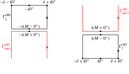
Figure 2: Definition of the integration curve $\Gamma_{\mathrm{tot}}=\Gamma_{\uparrow}\cup\Gamma_{\downarrow}$.

Further, given integers $n_{p/h}^{(\pm)}$, $n_{p/h}^{(M)}$ satisfying

$$n_{p}^{(+)}+n_{p}^{(-)}+n_{p}^{(M)}\,=\,n-1\qquad\mathrm{and}\qquad n_{h}^{(+)}+n_{h}^{(-)}+n_{h}^{(M)}\,=\,n\;,$$ (3.3)

we agree to denote

$$\boldsymbol{n}_{p}\,=\,\big{(}n_{p}^{(-)},n_{p}^{(+)},n_{p}^{(M)}\big{)}^{\boldsymbol{\texttt{t}}}\qquad\mathrm{as}\;\mathrm{well}\;\mathrm{as}\qquad\boldsymbol{n}_{h}\,=\,\big{(}n_{h}^{(-)},n_{h}^{(+)},n_{h}^{(M)}\big{)}^{\boldsymbol{\texttt{t}}}\;.$$ (3.4)

Then we define the associated contour

$$\mathscr{C}_{\boldsymbol{n}_{p},\boldsymbol{n}_{h}}\;=\;\Psi_{n}^{-1}\bigg{(}\Big{\{}\big{\{}\Gamma_{\downarrow}^{(M)}\big{\}}^{n_{p}^{(-)}}\times\big{\{}\Gamma_{\uparrow}^{(M)}\big{\}}^{n_{p}^{(+)}}\times\big{\{}\Gamma_{\mathrm{out}}^{(M)}\big{\}}^{n_{p}^{(M)}}\Big{\}}\times\Big{\{}\big{\{}\Gamma_{\uparrow}^{(M)}\big{\}}^{n_{h}^{(-)}}\times\big{\{}\Gamma_{\downarrow}^{(M)}\big{\}}^{n_{h}^{(+)}}\times\big{\{}\Gamma_{\mathrm{out}}^{(M)}\big{\}}^{n_{h}^{(M)}}\Big{\}}\bigg{)}$$ (3.5)

with $\Psi_{n}$ as defined in (2.30).

Also, for short, we introduce the functions

$$\mathcal{F}(\boldsymbol{w})\;=\;{\mathchoice{\dfrac{\mathscr{A}^{-+}\big{(}\boldsymbol{w}\big{)}\cdot\mathrm{e}^{\,\mathrm{i}m\Delta(\boldsymbol{w})}}{\prod\limits_{a=1}^{n-1}\Big{[}1\,+\,\mathrm{e}^{-\frac{1}{T}u(y_{a}\mid\,\boldsymbol{w})}\Big{]}\cdot\prod\limits_{a=1}^{n}\Big{[}1\,+\,\mathrm{e}^{\frac{1}{T}u(x_{a}\mid\,\boldsymbol{w})}\Big{]}}}{\dfrac{\mathscr{A}^{-+}\big{(}\boldsymbol{w}\big{)}\cdot\mathrm{e}^{\,\mathrm{i}m\Delta(\boldsymbol{w})}}{\prod\limits_{a=1}^{n-1}\Big{[}1\,+\,\mathrm{e}^{-\frac{1}{T}u(y_{a}\mid\,\boldsymbol{w})}\Big{]}\cdot\prod\limits_{a=1}^{n}\Big{[}1\,+\,\mathrm{e}^{\frac{1}{T}u(x_{a}\mid\,\boldsymbol{w})}\Big{]}}}{\frac{\mathscr{A}^{-+}\big{(}\boldsymbol{w}\big{)}\cdot\mathrm{e}^{\,\mathrm{i}m\Delta(\boldsymbol{w})}}{\prod\limits_{a=1}^{n-1}\Big{[}1\,+\,\mathrm{e}^{-\frac{1}{T}u(y_{a}\mid\,\boldsymbol{w})}\Big{]}\cdot\prod\limits_{a=1}^{n}\Big{[}1\,+\,\mathrm{e}^{\frac{1}{T}u(x_{a}\mid\,\boldsymbol{w})}\Big{]}}}{\frac{\mathscr{A}^{-+}\big{(}\boldsymbol{w}\big{)}\cdot\mathrm{e}^{\,\mathrm{i}m\Delta(\boldsymbol{w})}}{\prod\limits_{a=1}^{n-1}\Big{[}1\,+\,\mathrm{e}^{-\frac{1}{T}u(y_{a}\mid\,\boldsymbol{w})}\Big{]}\cdot\prod\limits_{a=1}^{n}\Big{[}1\,+\,\mathrm{e}^{\frac{1}{T}u(x_{a}\mid\,\boldsymbol{w})}\Big{]}}}}\;.$$ (3.6)

Then, the symmetry properties of $\mathcal{F}$ lead to the expansion

$$\int\limits_{\mathscr{C}_{n}}{\mathchoice{\dfrac{\mathrm{d}^{2n-1}w}{(2\mathrm{i}\pi)^{2n-1}}}{\dfrac{\mathrm{d}^{2n-1}w}{(2\mathrm{i}\pi)^{2n-1}}}{\frac{\mathrm{d}^{2n-1}w}{(2\mathrm{i}\pi)^{2n-1}}}{\frac{\mathrm{d}^{2n-1}w}{(2\mathrm{i}\pi)^{2n-1}}}}\mathcal{F}(\boldsymbol{w})\;=\;\sum\limits_{\begin{subarray}{c}n_{p}^{(-)}+n_{p}^{(+)}\\ +n_{p}^{(M)}=n-1\end{subarray}}\sum\limits_{\begin{subarray}{c}n_{h}^{(-)}+n_{h}^{(+)}\\ +n_{h}^{(M)}=n\end{subarray}}{\mathchoice{\dfrac{n!(n-1)!}{\prod\limits_{\upsilon\in\{\pm,M\}}n_{h}^{(\upsilon)}!\,n_{p}^{(\upsilon)}!}}{\dfrac{n!(n-1)!}{\prod\limits_{\upsilon\in\{\pm,M\}}n_{h}^{(\upsilon)}!\,n_{p}^{(\upsilon)}!}}{\frac{n!(n-1)!}{\prod\limits_{\upsilon\in\{\pm,M\}}n_{h}^{(\upsilon)}!\,n_{p}^{(\upsilon)}!}}{\frac{n!(n-1)!}{\prod\limits_{\upsilon\in\{\pm,M\}}n_{h}^{(\upsilon)}!\,n_{p}^{(\upsilon)}!}}}\int\limits_{\mathscr{C}_{\boldsymbol{n}_{p},\boldsymbol{n}_{h}}}\prod\limits_{\upsilon\in\{\pm,M\}}\bigg{\{}{\mathchoice{\dfrac{\mathrm{d}^{n_{p}^{(\upsilon)}}y^{(\upsilon)}}{(2\mathrm{i}\pi)^{n_{p}^{(\upsilon)}}}}{\dfrac{\mathrm{d}^{n_{p}^{(\upsilon)}}y^{(\upsilon)}}{(2\mathrm{i}\pi)^{n_{p}^{(\upsilon)}}}}{\frac{\mathrm{d}^{n_{p}^{(\upsilon)}}y^{(\upsilon)}}{(2\mathrm{i}\pi)^{n_{p}^{(\upsilon)}}}}{\frac{\mathrm{d}^{n_{p}^{(\upsilon)}}y^{(\upsilon)}}{(2\mathrm{i}\pi)^{n_{p}^{(\upsilon)}}}}}\cdot{\mathchoice{\dfrac{\mathrm{d}^{n_{h}^{(\upsilon)}}x^{(\upsilon)}}{(2\mathrm{i}\pi)^{n_{h}^{(\upsilon)}}}}{\dfrac{\mathrm{d}^{n_{h}^{(\upsilon)}}x^{(\upsilon)}}{(2\mathrm{i}\pi)^{n_{h}^{(\upsilon)}}}}{\frac{\mathrm{d}^{n_{h}^{(\upsilon)}}x^{(\upsilon)}}{(2\mathrm{i}\pi)^{n_{h}^{(\upsilon)}}}}{\frac{\mathrm{d}^{n_{h}^{(\upsilon)}}x^{(\upsilon)}}{(2\mathrm{i}\pi)^{n_{h}^{(\upsilon)}}}}}\bigg{\}}\cdot\mathcal{F}(\boldsymbol{\varpi})\;.$$ (3.7)

The variable $\boldsymbol{w}$ appearing in the lhs is as introduced in (2.26), while

$$\boldsymbol{\varpi}\;=\;\big{(}\widetilde{\boldsymbol{x}}_{n},\widetilde{\boldsymbol{y}}_{n-1}\big{)}^{\boldsymbol{\texttt{t}}}$$ (3.8)

appearing in the rhs is built from vectors $\widetilde{\boldsymbol{x}}_{n}$ and $\widetilde{\boldsymbol{y}}_{n-1}$ defined by

$$\widetilde{\boldsymbol{x}}_{n}\,=\,\Big{(}\boldsymbol{x}_{n_{h}^{(-)}}^{(-)},\boldsymbol{x}_{n_{h}^{(+)}}^{(+)},\boldsymbol{x}_{n_{h}^{(M)}}^{(M)}\Big{)}^{\boldsymbol{\texttt{t}}}\qquad\mathrm{and}\qquad\widetilde{\boldsymbol{y}}_{n-1}\,=\,\Big{(}\boldsymbol{y}_{n_{p}^{(-)}}^{(-)},\boldsymbol{y}_{n_{p}^{(+)}}^{(+)},\boldsymbol{y}_{n_{p}^{(M)}}^{(M)}\Big{)}^{\boldsymbol{\texttt{t}}}\;,$$ (3.9)

where

$$\boldsymbol{x}_{n_{h}^{(\upsilon)}}^{(\upsilon)}\,=\,\Big{(}x_{1}^{(\upsilon)},\dots,x_{n_{h}^{(\upsilon)}}^{(\upsilon)}\Big{)}^{\boldsymbol{\texttt{t}}}\qquad\mathrm{and}\qquad\boldsymbol{y}_{n_{p}^{(\upsilon)}}^{(\upsilon)}\,=\,\Big{(}y_{1}^{(\upsilon)},\dots,y_{n_{p}^{(\upsilon)}}^{(\upsilon)}\Big{)}^{\boldsymbol{\texttt{t}}}\;,\qquad\mathrm{with}\qquad\upsilon\in\{\pm,M\}\;.$$ (3.10)

The integrals emerging from the preimages of the contours $\Gamma_{\uparrow/\downarrow}^{(M)}$ can be taken explicitly by residue calculations. For that purpose, we need to introduce several notations. First of all, consider the vectors

$$\boldsymbol{p}_{n_{p}^{(\sigma)}}^{(\sigma)}\;=\;\Big{(}p_{1}^{(\sigma)},\dots,p_{n_{p}^{(\sigma)}}^{(\sigma)}\Big{)}^{\boldsymbol{\texttt{t}}}\qquad\mathrm{and}\qquad\boldsymbol{h}_{n_{h}^{(\sigma)}}^{(\sigma)}\;=\;\Big{(}h_{1}^{(\sigma)},\dots,h_{n_{h}^{(\sigma)}}^{(\sigma)}\Big{)}^{\boldsymbol{\texttt{t}}}\;,$$ (3.11)

with $\sigma\in\big{\{}\pm\big{\}}$, whose coordinates are integers satisfying the constraints

$$0\leq p_{1}^{(\sigma)}<\cdots<p_{n_{p}^{(\sigma)}}^{(\sigma)}\leq M-1\;,\qquad 0\leq h_{1}^{(\sigma)}<\cdots<h_{n_{h}^{(\sigma)}}^{(\sigma)}\leq M-1\;.$$ (3.12)

It is further convenient to denote $\boldsymbol{p}=\big{(}\boldsymbol{p}_{n_{p}^{(-)}}^{(-)},\boldsymbol{p}_{n_{p}^{(+)}}^{(+)}\big{)}^{\boldsymbol{\texttt{t}}}$ , $\boldsymbol{h}=\big{(}\boldsymbol{h}_{n_{h}^{(-)}}^{(-)},\boldsymbol{h}_{n_{h}^{(+)}}^{(+)}\big{)}^{\boldsymbol{\texttt{t}}}$. Next, for fixed vectors $\boldsymbol{y}_{n_{p}^{(M)}}^{(M)},\boldsymbol{x}_{n_{h}^{(M)}}^{(M)}$, we introduce the unique solution $\boldsymbol{\texttt{y}}_{a}^{(\sigma)},\boldsymbol{\texttt{x}}_{a}^{(\sigma)}$, belonging to a neighbourhood of $\sigma q$, to the equations

$$\begin{array}[]{ccc}u\big{(}\boldsymbol{\texttt{x}}_{a}^{(\sigma)}\mid\boldsymbol{\varpi}_{\boldsymbol{p},\boldsymbol{h}}\big{)}\;=\;-\sigma 2\mathrm{i}\pi T\big{(}h_{a}^{(\sigma)}+\tfrac{1}{2}\big{)}&,&a=1,\dots,n_{h}^{(\sigma)}\vspace{2mm}\\ u\big{(}\boldsymbol{\texttt{y}}_{a}^{(\sigma)}\mid\boldsymbol{\varpi}_{\boldsymbol{p},\boldsymbol{h}}\big{)}\;=\;\sigma 2\mathrm{i}\pi T\big{(}p_{a}^{(\sigma)}+\tfrac{1}{2}\big{)}&,&a=1,\dots,n_{p}^{(\sigma)}\end{array}\;,$$ (3.13)

where

$$\boldsymbol{\varpi}_{\boldsymbol{p},\boldsymbol{h}}\;=\;\Big{(}\boldsymbol{\texttt{x}}_{n_{h}^{(-)}}^{(-)},\boldsymbol{\texttt{x}}_{n_{h}^{(+)}}^{(+)},\boldsymbol{x}_{n_{h}^{(M)}}^{(M)};\boldsymbol{\texttt{y}}_{n_{p}^{(-)}}^{(-)},\boldsymbol{\texttt{y}}_{n_{p}^{(+)}}^{(+)},\boldsymbol{y}_{n_{p}^{(M)}}^{(M)}\Big{)}^{\boldsymbol{\texttt{t}}}$$ (3.14)

and

$$\boldsymbol{\boldsymbol{\texttt{y}}}_{n_{p}^{(\sigma)}}^{(\sigma)}\;=\;\Big{(}\boldsymbol{\texttt{y}}_{1}^{(\sigma)},\dots,\boldsymbol{\texttt{y}}_{n_{p}^{(\sigma)}}^{(\sigma)}\Big{)}^{\boldsymbol{\texttt{t}}}\qquad\mathrm{and}\qquad\boldsymbol{\boldsymbol{\texttt{x}}}_{n_{h}^{(\sigma)}}^{(\sigma)}\;=\;\Big{(}\boldsymbol{\texttt{x}}_{1}^{(\sigma)},\dots,\boldsymbol{\texttt{x}}_{n_{h}^{(\sigma)}}^{(\sigma)}\Big{)}^{\boldsymbol{\texttt{t}}}\;.$$ (3.15)

The existence and uniqueness of such solutions follows from the work [11].

We now factorise $\mathcal{F}\big{(}\boldsymbol{\varpi}\big{)}$ as

$$\mathcal{F}(\boldsymbol{\varpi})\;=\;{\mathchoice{\dfrac{\operatorname{det}\Big{[}\boldsymbol{\texttt{D}}\Psi_{n}(\boldsymbol{\varpi})\Big{]}\cdot\mathcal{G}(\boldsymbol{\varpi})}{\prod\limits_{\sigma=\pm}\prod\limits_{a=1}^{n_{p}^{(\sigma)}}\Big{[}1\,+\,\mathrm{e}^{-\frac{1}{T}u(y_{a}^{(\sigma)}\,\mid\,\boldsymbol{w})}\Big{]}\cdot\prod\limits_{\sigma=\pm}\prod\limits_{a=1}^{n_{h}^{(\sigma)}}\Big{[}1\,+\,\mathrm{e}^{\frac{1}{T}u(x_{a}^{(\sigma)}\,\mid\,\boldsymbol{w})}\Big{]}}}{\dfrac{\operatorname{det}\Big{[}\boldsymbol{\texttt{D}}\Psi_{n}(\boldsymbol{\varpi})\Big{]}\cdot\mathcal{G}(\boldsymbol{\varpi})}{\prod\limits_{\sigma=\pm}\prod\limits_{a=1}^{n_{p}^{(\sigma)}}\Big{[}1\,+\,\mathrm{e}^{-\frac{1}{T}u(y_{a}^{(\sigma)}\,\mid\,\boldsymbol{w})}\Big{]}\cdot\prod\limits_{\sigma=\pm}\prod\limits_{a=1}^{n_{h}^{(\sigma)}}\Big{[}1\,+\,\mathrm{e}^{\frac{1}{T}u(x_{a}^{(\sigma)}\,\mid\,\boldsymbol{w})}\Big{]}}}{\frac{\operatorname{det}\Big{[}\boldsymbol{\texttt{D}}\Psi_{n}(\boldsymbol{\varpi})\Big{]}\cdot\mathcal{G}(\boldsymbol{\varpi})}{\prod\limits_{\sigma=\pm}\prod\limits_{a=1}^{n_{p}^{(\sigma)}}\Big{[}1\,+\,\mathrm{e}^{-\frac{1}{T}u(y_{a}^{(\sigma)}\,\mid\,\boldsymbol{w})}\Big{]}\cdot\prod\limits_{\sigma=\pm}\prod\limits_{a=1}^{n_{h}^{(\sigma)}}\Big{[}1\,+\,\mathrm{e}^{\frac{1}{T}u(x_{a}^{(\sigma)}\,\mid\,\boldsymbol{w})}\Big{]}}}{\frac{\operatorname{det}\Big{[}\boldsymbol{\texttt{D}}\Psi_{n}(\boldsymbol{\varpi})\Big{]}\cdot\mathcal{G}(\boldsymbol{\varpi})}{\prod\limits_{\sigma=\pm}\prod\limits_{a=1}^{n_{p}^{(\sigma)}}\Big{[}1\,+\,\mathrm{e}^{-\frac{1}{T}u(y_{a}^{(\sigma)}\,\mid\,\boldsymbol{w})}\Big{]}\cdot\prod\limits_{\sigma=\pm}\prod\limits_{a=1}^{n_{h}^{(\sigma)}}\Big{[}1\,+\,\mathrm{e}^{\frac{1}{T}u(x_{a}^{(\sigma)}\,\mid\,\boldsymbol{w})}\Big{]}}}}$$ (3.16)

in which

$$\mathcal{G}(\boldsymbol{\varpi})\;=\;{\mathchoice{\dfrac{\mathscr{A}^{-+}\big{(}\boldsymbol{\varpi}\big{)}\cdot\mathrm{e}^{\,\mathrm{i}m\Delta(\boldsymbol{\varpi})}}{\operatorname{det}\Big{[}\boldsymbol{\texttt{D}}\Psi_{n}(\boldsymbol{\varpi})\Big{]}}}{\dfrac{\mathscr{A}^{-+}\big{(}\boldsymbol{\varpi}\big{)}\cdot\mathrm{e}^{\,\mathrm{i}m\Delta(\boldsymbol{\varpi})}}{\operatorname{det}\Big{[}\boldsymbol{\texttt{D}}\Psi_{n}(\boldsymbol{\varpi})\Big{]}}}{\frac{\mathscr{A}^{-+}\big{(}\boldsymbol{\varpi}\big{)}\cdot\mathrm{e}^{\,\mathrm{i}m\Delta(\boldsymbol{\varpi})}}{\operatorname{det}\Big{[}\boldsymbol{\texttt{D}}\Psi_{n}(\boldsymbol{\varpi})\Big{]}}}{\frac{\mathscr{A}^{-+}\big{(}\boldsymbol{\varpi}\big{)}\cdot\mathrm{e}^{\,\mathrm{i}m\Delta(\boldsymbol{\varpi})}}{\operatorname{det}\Big{[}\boldsymbol{\texttt{D}}\Psi_{n}(\boldsymbol{\varpi})\Big{]}}}}\cdot\prod\limits_{a=1}^{n_{p}^{(M)}}\bigg{\{}{\mathchoice{\dfrac{1}{1\,+\,\mathrm{e}^{-\frac{1}{T}u(y_{a}^{(M)}\mid\,\boldsymbol{\varpi})}}}{\dfrac{1}{1\,+\,\mathrm{e}^{-\frac{1}{T}u(y_{a}^{(M)}\mid\,\boldsymbol{\varpi})}}}{\frac{1}{1\,+\,\mathrm{e}^{-\frac{1}{T}u(y_{a}^{(M)}\mid\,\boldsymbol{\varpi})}}}{\frac{1}{1\,+\,\mathrm{e}^{-\frac{1}{T}u(y_{a}^{(M)}\mid\,\boldsymbol{\varpi})}}}}\bigg{\}}\cdot\prod\limits_{a=1}^{n_{h}^{(M)}}\bigg{\{}{\mathchoice{\dfrac{1}{1\,+\,\mathrm{e}^{\frac{1}{T}u(x_{a}^{(M)}\mid\,\boldsymbol{\varpi})}}}{\dfrac{1}{1\,+\,\mathrm{e}^{\frac{1}{T}u(x_{a}^{(M)}\mid\,\boldsymbol{\varpi})}}}{\frac{1}{1\,+\,\mathrm{e}^{\frac{1}{T}u(x_{a}^{(M)}\mid\,\boldsymbol{\varpi})}}}{\frac{1}{1\,+\,\mathrm{e}^{\frac{1}{T}u(x_{a}^{(M)}\mid\,\boldsymbol{\varpi})}}}}\bigg{\}}\;.$$ (3.17)

All of the above leads to

$$\mathcal{J}_{\boldsymbol{n}_{p},\boldsymbol{n}_{h}}\;=\;\int\limits_{\mathscr{C}_{\boldsymbol{n}_{p},\boldsymbol{n}_{h}}}\prod\limits_{\upsilon\in\{\pm,M\}}\bigg{\{}{\mathchoice{\dfrac{\mathrm{d}^{n_{p}^{(\upsilon)}}y^{(\upsilon)}}{(2\mathrm{i}\pi)^{n_{p}^{(\upsilon)}}}}{\dfrac{\mathrm{d}^{n_{p}^{(\upsilon)}}y^{(\upsilon)}}{(2\mathrm{i}\pi)^{n_{p}^{(\upsilon)}}}}{\frac{\mathrm{d}^{n_{p}^{(\upsilon)}}y^{(\upsilon)}}{(2\mathrm{i}\pi)^{n_{p}^{(\upsilon)}}}}{\frac{\mathrm{d}^{n_{p}^{(\upsilon)}}y^{(\upsilon)}}{(2\mathrm{i}\pi)^{n_{p}^{(\upsilon)}}}}}\cdot{\mathchoice{\dfrac{\mathrm{d}^{n_{h}^{(\upsilon)}}x^{(\upsilon)}}{(2\mathrm{i}\pi)^{n_{h}^{(\upsilon)}}}}{\dfrac{\mathrm{d}^{n_{h}^{(\upsilon)}}x^{(\upsilon)}}{(2\mathrm{i}\pi)^{n_{h}^{(\upsilon)}}}}{\frac{\mathrm{d}^{n_{h}^{(\upsilon)}}x^{(\upsilon)}}{(2\mathrm{i}\pi)^{n_{h}^{(\upsilon)}}}}{\frac{\mathrm{d}^{n_{h}^{(\upsilon)}}x^{(\upsilon)}}{(2\mathrm{i}\pi)^{n_{h}^{(\upsilon)}}}}}\bigg{\}}\cdot\mathcal{F}(\boldsymbol{\varpi})\;=\int\limits_{\Gamma_{\mathrm{out}}^{(M)}}{\mathchoice{\dfrac{\mathrm{d}^{n_{p}^{(M)}}z^{(M)}}{(2\mathrm{i}\pi)^{n_{p}^{(M)}}}}{\dfrac{\mathrm{d}^{n_{p}^{(M)}}z^{(M)}}{(2\mathrm{i}\pi)^{n_{p}^{(M)}}}}{\frac{\mathrm{d}^{n_{p}^{(M)}}z^{(M)}}{(2\mathrm{i}\pi)^{n_{p}^{(M)}}}}{\frac{\mathrm{d}^{n_{p}^{(M)}}z^{(M)}}{(2\mathrm{i}\pi)^{n_{p}^{(M)}}}}}\int\limits_{\Gamma_{\mathrm{out}}^{(M)}}{\mathchoice{\dfrac{\mathrm{d}^{n_{h}^{(M)}}\mathfrak{z}^{(M)}}{(2\mathrm{i}\pi)^{n_{h}^{(M)}}}}{\dfrac{\mathrm{d}^{n_{h}^{(M)}}\mathfrak{z}^{(M)}}{(2\mathrm{i}\pi)^{n_{h}^{(M)}}}}{\frac{\mathrm{d}^{n_{h}^{(M)}}\mathfrak{z}^{(M)}}{(2\mathrm{i}\pi)^{n_{h}^{(M)}}}}{\frac{\mathrm{d}^{n_{h}^{(M)}}\mathfrak{z}^{(M)}}{(2\mathrm{i}\pi)^{n_{h}^{(M)}}}}}\\ \times\int\limits_{\Gamma_{\downarrow}^{(M)}}{\mathchoice{\dfrac{\mathrm{d}^{n_{p}^{(-)}}z^{(-)}}{(2\mathrm{i}\pi)^{n_{p}^{(-)}}}}{\dfrac{\mathrm{d}^{n_{p}^{(-)}}z^{(-)}}{(2\mathrm{i}\pi)^{n_{p}^{(-)}}}}{\frac{\mathrm{d}^{n_{p}^{(-)}}z^{(-)}}{(2\mathrm{i}\pi)^{n_{p}^{(-)}}}}{\frac{\mathrm{d}^{n_{p}^{(-)}}z^{(-)}}{(2\mathrm{i}\pi)^{n_{p}^{(-)}}}}}\int\limits_{\Gamma_{\uparrow}^{(M)}}{\mathchoice{\dfrac{\mathrm{d}^{n_{h}^{(-)}}\mathfrak{z}^{(-)}}{(2\mathrm{i}\pi)^{n_{h}^{(-)}}}}{\dfrac{\mathrm{d}^{n_{h}^{(-)}}\mathfrak{z}^{(-)}}{(2\mathrm{i}\pi)^{n_{h}^{(-)}}}}{\frac{\mathrm{d}^{n_{h}^{(-)}}\mathfrak{z}^{(-)}}{(2\mathrm{i}\pi)^{n_{h}^{(-)}}}}{\frac{\mathrm{d}^{n_{h}^{(-)}}\mathfrak{z}^{(-)}}{(2\mathrm{i}\pi)^{n_{h}^{(-)}}}}}\int\limits_{\Gamma_{\uparrow}^{(M)}}{\mathchoice{\dfrac{\mathrm{d}^{n_{p}^{(+)}}z^{(+)}}{(2\mathrm{i}\pi)^{n_{p}^{(+)}}}}{\dfrac{\mathrm{d}^{n_{p}^{(+)}}z^{(+)}}{(2\mathrm{i}\pi)^{n_{p}^{(+)}}}}{\frac{\mathrm{d}^{n_{p}^{(+)}}z^{(+)}}{(2\mathrm{i}\pi)^{n_{p}^{(+)}}}}{\frac{\mathrm{d}^{n_{p}^{(+)}}z^{(+)}}{(2\mathrm{i}\pi)^{n_{p}^{(+)}}}}}\int\limits_{\Gamma_{\downarrow}^{(M)}}{\mathchoice{\dfrac{\mathrm{d}^{n_{h}^{(+)}}\mathfrak{z}^{(+)}}{(2\mathrm{i}\pi)^{n_{h}^{(+)}}}}{\dfrac{\mathrm{d}^{n_{h}^{(+)}}\mathfrak{z}^{(+)}}{(2\mathrm{i}\pi)^{n_{h}^{(+)}}}}{\frac{\mathrm{d}^{n_{h}^{(+)}}\mathfrak{z}^{(+)}}{(2\mathrm{i}\pi)^{n_{h}^{(+)}}}}{\frac{\mathrm{d}^{n_{h}^{(+)}}\mathfrak{z}^{(+)}}{(2\mathrm{i}\pi)^{n_{h}^{(+)}}}}}{\mathchoice{\dfrac{\mathcal{G}\circ\Psi_{n}^{-1}\big{(}\boldsymbol{Z}\big{)}}{\prod\limits_{\sigma=\pm}\prod\limits_{a=1}^{n_{p}^{(\sigma)}}\Big{[}1\,+\,\mathrm{e}^{-\frac{1}{T}z^{(\sigma)}}\Big{]}\cdot\prod\limits_{\sigma=\pm}\prod\limits_{a=1}^{n_{h}^{(\sigma)}}\Big{[}1\,+\,\mathrm{e}^{\frac{1}{T}\mathfrak{z}^{(\sigma)}}\Big{]}}}{\dfrac{\mathcal{G}\circ\Psi_{n}^{-1}\big{(}\boldsymbol{Z}\big{)}}{\prod\limits_{\sigma=\pm}\prod\limits_{a=1}^{n_{p}^{(\sigma)}}\Big{[}1\,+\,\mathrm{e}^{-\frac{1}{T}z^{(\sigma)}}\Big{]}\cdot\prod\limits_{\sigma=\pm}\prod\limits_{a=1}^{n_{h}^{(\sigma)}}\Big{[}1\,+\,\mathrm{e}^{\frac{1}{T}\mathfrak{z}^{(\sigma)}}\Big{]}}}{\frac{\mathcal{G}\circ\Psi_{n}^{-1}\big{(}\boldsymbol{Z}\big{)}}{\prod\limits_{\sigma=\pm}\prod\limits_{a=1}^{n_{p}^{(\sigma)}}\Big{[}1\,+\,\mathrm{e}^{-\frac{1}{T}z^{(\sigma)}}\Big{]}\cdot\prod\limits_{\sigma=\pm}\prod\limits_{a=1}^{n_{h}^{(\sigma)}}\Big{[}1\,+\,\mathrm{e}^{\frac{1}{T}\mathfrak{z}^{(\sigma)}}\Big{]}}}{\frac{\mathcal{G}\circ\Psi_{n}^{-1}\big{(}\boldsymbol{Z}\big{)}}{\prod\limits_{\sigma=\pm}\prod\limits_{a=1}^{n_{p}^{(\sigma)}}\Big{[}1\,+\,\mathrm{e}^{-\frac{1}{T}z^{(\sigma)}}\Big{]}\cdot\prod\limits_{\sigma=\pm}\prod\limits_{a=1}^{n_{h}^{(\sigma)}}\Big{[}1\,+\,\mathrm{e}^{\frac{1}{T}\mathfrak{z}^{(\sigma)}}\Big{]}}}}\;,$$ (3.18)

where we have introduced the vector

$$\boldsymbol{Z}\;=\;\Big{(}\big{(}\boldsymbol{z}^{(-)}_{n_{p}^{(-)}},\boldsymbol{z}^{(+)}_{n_{p}^{(+)}},\boldsymbol{z}^{(M)}_{n_{p}^{(M)}}\big{)},\big{(}\boldsymbol{\mathfrak{z}}^{(-)}_{n_{p}^{(-)}},\boldsymbol{\mathfrak{z}}^{(+)}_{n_{p}^{(+)}},\boldsymbol{\mathfrak{z}}^{(M)}_{n_{p}^{(M)}}\big{)}\Big{)}^{\boldsymbol{\texttt{t}}}\;.$$ (3.19)

One may now take the integrals occurring in the second line of (3.18) in terms of residues at the simple poles

$$z_{a}^{(\sigma)}\,=\,2\mathrm{i}\pi\sigma\Big{(}p_{a}^{(\sigma)}+{\mathchoice{\dfrac{1}{2}}{\dfrac{1}{2}}{\frac{1}{2}}{\frac{1}{2}}}\Big{)}\qquad\mathrm{and}\qquad\mathfrak{z}_{a}^{(\sigma)}\,=\,-2\mathrm{i}\pi\sigma\Big{(}h_{a}^{(\sigma)}+{\mathchoice{\dfrac{1}{2}}{\dfrac{1}{2}}{\frac{1}{2}}{\frac{1}{2}}}\Big{)}$$ (3.20)

where

$$h_{a}^{(\sigma)},p_{a}^{(\sigma)}\in[\![\,0\,;\,M-1\,]\!]\;.$$ (3.21)

Thus, computing the residues will lead, in principle, to a summation over all choices of such integers. Still, some simplifications are possible. Indeed, $\mathscr{A}^{-+}\circ\Psi_{n}(\boldsymbol{Z})$ vanishes as soon as two variables of $y$ or two of $x$ type coincide. It was established in [11] that solutions to (3.13) which would be subordinate to some choices of integers such that $h_{a}^{(\sigma)}=h_{b}^{(\sigma)}$ or $p_{a}^{(\sigma)}=p_{b}^{(\sigma)}$ for some $a\not=b$ exhibit coinciding coordinates. Thus, one only needs to sum over choices of pairwise distinct integers $h_{a}^{(\sigma)}$ or $p_{a}^{(\sigma)}$ as the other contributions vanish. Moreover, given a point $\boldsymbol{Z}_{\boldsymbol{p},\boldsymbol{h}}$ computed at the residue coordinates given in (3.20), viz. $\boldsymbol{Z}_{\boldsymbol{p},\boldsymbol{h}}$ is as given in (3.19) in which the coordinates of the vectors $\boldsymbol{z}^{(\pm)}_{n_{p}^{(\pm)}},\boldsymbol{\mathfrak{z}}^{(\pm)}_{n_{p}^{(\pm)}}$ are given by (3.20), we observe that any permutation of the indices of $h_{a}^{(\sigma)}$ or $p_{a}^{(\sigma)}$ will lead to a permutation of the associated $"y"$ or $"x"$ type coordinates in $\Psi_{n}^{-1}(\boldsymbol{Z}_{\boldsymbol{p},\boldsymbol{h}})$, hence leaving the value of $\mathcal{G}\circ\Psi_{n}^{-1}\big{(}\boldsymbol{Z}_{\boldsymbol{p},\boldsymbol{h}}\big{)}$ invariant, owing to the permutation invariance of $\mathcal{G}$. Thus, up to combinatorial factors, one may reduce the summations over

$$0\leq h_{1}^{(\sigma)}\not=\cdots\not=h_{n_{h}^{(\sigma)}}^{(\sigma)}\leq M-1\;,\qquad 0\leq p_{1}^{(\sigma)}\not=\cdots\not=p_{n_{p}^{(\sigma)}}^{(\sigma)}\leq M-1\;,$$ (3.22)

to the ordered ones

$$0\leq h_{1}^{(\sigma)}<\cdots<h_{n_{h}^{(\sigma)}}^{(\sigma)}\leq M-1,\qquad 0\leq p_{1}^{(\sigma)}<\cdots<p_{n_{p}^{(\sigma)}}^{(\sigma)}\leq M-1\;.$$ (3.23)

The above leads to

$$\mathcal{J}_{\boldsymbol{n}_{p},\boldsymbol{n}_{h}}\;=\;\int\limits_{\Gamma_{\mathrm{out}}^{(M)}}{\mathchoice{\dfrac{\mathrm{d}^{n_{p}^{(M)}}z^{(M)}}{(2\mathrm{i}\pi)^{n_{p}^{(M)}}}}{\dfrac{\mathrm{d}^{n_{p}^{(M)}}z^{(M)}}{(2\mathrm{i}\pi)^{n_{p}^{(M)}}}}{\frac{\mathrm{d}^{n_{p}^{(M)}}z^{(M)}}{(2\mathrm{i}\pi)^{n_{p}^{(M)}}}}{\frac{\mathrm{d}^{n_{p}^{(M)}}z^{(M)}}{(2\mathrm{i}\pi)^{n_{p}^{(M)}}}}}\int\limits_{\Gamma_{\mathrm{out}}^{(M)}}{\mathchoice{\dfrac{\mathrm{d}^{n_{h}^{(M)}}\mathfrak{z}^{(M)}}{(2\mathrm{i}\pi)^{n_{h}^{(M)}}}}{\dfrac{\mathrm{d}^{n_{h}^{(M)}}\mathfrak{z}^{(M)}}{(2\mathrm{i}\pi)^{n_{h}^{(M)}}}}{\frac{\mathrm{d}^{n_{h}^{(M)}}\mathfrak{z}^{(M)}}{(2\mathrm{i}\pi)^{n_{h}^{(M)}}}}{\frac{\mathrm{d}^{n_{h}^{(M)}}\mathfrak{z}^{(M)}}{(2\mathrm{i}\pi)^{n_{h}^{(M)}}}}}\prod\limits_{\sigma=\pm}\Bigg{\{}(-T)^{n_{h}^{(\sigma)}}\cdot n_{h}^{(\sigma)}!\sum\limits_{0\leq h_{1}^{(\sigma)}<\cdots<h_{n_{h}^{(\sigma)}}^{(\sigma)}}^{M-1}T^{n_{p}^{(\sigma)}}\cdot n_{p}^{(\sigma)}!\sum\limits_{0\leq p_{1}^{(\sigma)}<\cdots<p_{n_{p}^{(\sigma)}}^{(\sigma)}}^{M-1}\Bigg{\}}\mathcal{G}\Big{(}\Psi_{n}^{-1}(\boldsymbol{Z}_{\boldsymbol{p},\boldsymbol{h}})\Big{)}\;.$$ (3.24)

At this stage one makes the change of integration variables

$$\Big{(}\boldsymbol{x}_{n_{h}^{(M)}}^{(M)},\boldsymbol{y}_{n_{p}^{(M)}}^{(M)}\Big{)}\;=\;\Psi_{n;\mathrm{out}}^{-1}\Big{(}\boldsymbol{z}^{(M)}_{n_{p}^{(M)}},\boldsymbol{\mathfrak{z}}^{(M)}_{n_{h}^{(M)}}\Big{)}$$ (3.25)

where the map $\Psi_{n;\mathrm{out}}$ is defined by

$$\Psi_{n;\mathrm{out}}\Big{(}\boldsymbol{x}_{n_{h}^{(M)}}^{(M)},\boldsymbol{y}_{n_{p}^{(M)}}^{(M)}\Big{)}\;=\;\Big{(}\psi^{(p)}\big{(}y_{1}^{(M)}\mid\boldsymbol{\varpi}_{\boldsymbol{p},\boldsymbol{h}}\big{)},\dots,\psi^{(p)}\big{(}y_{n_{p}^{(M)}}^{(M)}\mid\boldsymbol{\varpi}_{\boldsymbol{p},\boldsymbol{h}}\big{)},\psi^{(h)}\big{(}x_{1}^{(M)}\mid\boldsymbol{\varpi}_{\boldsymbol{p},\boldsymbol{h}}\big{)},\dots,\psi^{(h)}\big{(}x_{n_{h}^{(M)}}^{(M)}\mid\boldsymbol{\varpi}_{\boldsymbol{p},\boldsymbol{h}}\big{)}\Big{)}\;.$$ (3.26)

We recall that the functions $\psi^{(p/h)}$ have been introduced in (2.29) while $\boldsymbol{\varpi}_{\boldsymbol{p},\boldsymbol{h}}$ has been introduced in (3.14).

Then, upon introducing the integration contour

$$\mathscr{C}_{n_{p}^{(M)}\!\!,\,n_{h}^{(M)}}\;=\;\Psi_{n;\mathrm{out}}^{-1}\bigg{(}\big{\{}\Gamma_{\mathrm{out}}^{(M)}\big{\}}^{n_{p}^{(M)}}\times\big{\{}\Gamma_{\mathrm{out}}^{(M)}\big{\}}^{n_{h}^{(M)}}\bigg{)}\;,$$ (3.27)

one obtains the below representation for the two-point function:

$$\big{<}\sigma_{1}^{-}\sigma_{m+1}^{+}(t)\big{>}_{T}\,=\,\sum\limits_{n\geq 1}\sum\limits_{\begin{subarray}{c}n_{p}^{(-)}+n_{p}^{(+)}\\ +n_{p}^{(M)}=n-1\end{subarray}}\sum\limits_{\begin{subarray}{c}n_{h}^{(-)}+n_{h}^{(+)}\\ +n_{h}^{(M)}=n\end{subarray}}{\mathchoice{\dfrac{1}{n_{p}^{(M)}!\,n_{h}^{(M)}!}}{\dfrac{1}{n_{p}^{(M)}!\,n_{h}^{(M)}!}}{\frac{1}{n_{p}^{(M)}!\,n_{h}^{(M)}!}}{\frac{1}{n_{p}^{(M)}!\,n_{h}^{(M)}!}}}\prod\limits_{\sigma=\pm}\Bigg{\{}(-T)^{n_{h}^{(\sigma)}}\sum\limits_{0\leq h_{1}^{(\sigma)}<\cdots<h_{n_{h}^{(\sigma)}}^{(\sigma)}}^{M-1}T^{n_{p}^{(\sigma)}}\sum\limits_{0\leq p_{1}^{(\sigma)}<\cdots<p_{n_{p}^{(\sigma)}}^{(\sigma)}}^{M-1}\Bigg{\}}\\ \times\int\limits_{\mathscr{C}_{n_{p}^{(M)}\!\!,\,n_{h}^{(M)}}}{\mathchoice{\dfrac{\mathrm{d}^{n_{p}^{(M)}}y^{(M)}}{(2\mathrm{i}\pi)^{n_{p}^{(M)}}}}{\dfrac{\mathrm{d}^{n_{p}^{(M)}}y^{(M)}}{(2\mathrm{i}\pi)^{n_{p}^{(M)}}}}{\frac{\mathrm{d}^{n_{p}^{(M)}}y^{(M)}}{(2\mathrm{i}\pi)^{n_{p}^{(M)}}}}{\frac{\mathrm{d}^{n_{p}^{(M)}}y^{(M)}}{(2\mathrm{i}\pi)^{n_{p}^{(M)}}}}}\cdot{\mathchoice{\dfrac{\mathrm{d}^{n_{h}^{(M)}}x^{(M)}}{(2\mathrm{i}\pi)^{n_{h}^{(M)}}}}{\dfrac{\mathrm{d}^{n_{h}^{(M)}}x^{(M)}}{(2\mathrm{i}\pi)^{n_{h}^{(M)}}}}{\frac{\mathrm{d}^{n_{h}^{(M)}}x^{(M)}}{(2\mathrm{i}\pi)^{n_{h}^{(M)}}}}{\frac{\mathrm{d}^{n_{h}^{(M)}}x^{(M)}}{(2\mathrm{i}\pi)^{n_{h}^{(M)}}}}}{\mathchoice{\dfrac{\operatorname{det}\big{[}\boldsymbol{\texttt{D}}\Psi_{n;\mathrm{out}}(\boldsymbol{\varpi}_{\boldsymbol{p},\boldsymbol{h}})\big{]}}{\operatorname{det}\Big{[}\boldsymbol{\texttt{D}}\Psi_{n}(\boldsymbol{\varpi}_{\boldsymbol{p},\boldsymbol{h}})\Big{]}}}{\dfrac{\operatorname{det}\big{[}\boldsymbol{\texttt{D}}\Psi_{n;\mathrm{out}}(\boldsymbol{\varpi}_{\boldsymbol{p},\boldsymbol{h}})\big{]}}{\operatorname{det}\Big{[}\boldsymbol{\texttt{D}}\Psi_{n}(\boldsymbol{\varpi}_{\boldsymbol{p},\boldsymbol{h}})\Big{]}}}{\frac{\operatorname{det}\big{[}\boldsymbol{\texttt{D}}\Psi_{n;\mathrm{out}}(\boldsymbol{\varpi}_{\boldsymbol{p},\boldsymbol{h}})\big{]}}{\operatorname{det}\Big{[}\boldsymbol{\texttt{D}}\Psi_{n}(\boldsymbol{\varpi}_{\boldsymbol{p},\boldsymbol{h}})\Big{]}}}{\frac{\operatorname{det}\big{[}\boldsymbol{\texttt{D}}\Psi_{n;\mathrm{out}}(\boldsymbol{\varpi}_{\boldsymbol{p},\boldsymbol{h}})\big{]}}{\operatorname{det}\Big{[}\boldsymbol{\texttt{D}}\Psi_{n}(\boldsymbol{\varpi}_{\boldsymbol{p},\boldsymbol{h}})\Big{]}}}}\cdot{\mathchoice{\dfrac{(-1)^{m+n}\mathscr{A}^{-+}\big{(}\boldsymbol{\varpi}_{\boldsymbol{p},\boldsymbol{h}}\big{)}\cdot\mathrm{e}^{\,\mathrm{i}m\Delta(\boldsymbol{\varpi}_{\boldsymbol{p},\boldsymbol{h}})}}{\prod\limits_{a=1}^{n_{p}^{(M)}}\Big{[}1\,+\,\mathrm{e}^{-\frac{1}{T}u(y_{a}^{(M)}\mid\,\boldsymbol{\varpi}_{\boldsymbol{p},\boldsymbol{h}})}\Big{]}\cdot\prod\limits_{a=1}^{n_{h}^{(M)}}\Big{[}1\,+\,\mathrm{e}^{\frac{1}{T}u(x_{a}^{(M)}\mid\,\boldsymbol{\varpi}_{\boldsymbol{p},\boldsymbol{h}})}\Big{]}}}{\dfrac{(-1)^{m+n}\mathscr{A}^{-+}\big{(}\boldsymbol{\varpi}_{\boldsymbol{p},\boldsymbol{h}}\big{)}\cdot\mathrm{e}^{\,\mathrm{i}m\Delta(\boldsymbol{\varpi}_{\boldsymbol{p},\boldsymbol{h}})}}{\prod\limits_{a=1}^{n_{p}^{(M)}}\Big{[}1\,+\,\mathrm{e}^{-\frac{1}{T}u(y_{a}^{(M)}\mid\,\boldsymbol{\varpi}_{\boldsymbol{p},\boldsymbol{h}})}\Big{]}\cdot\prod\limits_{a=1}^{n_{h}^{(M)}}\Big{[}1\,+\,\mathrm{e}^{\frac{1}{T}u(x_{a}^{(M)}\mid\,\boldsymbol{\varpi}_{\boldsymbol{p},\boldsymbol{h}})}\Big{]}}}{\frac{(-1)^{m+n}\mathscr{A}^{-+}\big{(}\boldsymbol{\varpi}_{\boldsymbol{p},\boldsymbol{h}}\big{)}\cdot\mathrm{e}^{\,\mathrm{i}m\Delta(\boldsymbol{\varpi}_{\boldsymbol{p},\boldsymbol{h}})}}{\prod\limits_{a=1}^{n_{p}^{(M)}}\Big{[}1\,+\,\mathrm{e}^{-\frac{1}{T}u(y_{a}^{(M)}\mid\,\boldsymbol{\varpi}_{\boldsymbol{p},\boldsymbol{h}})}\Big{]}\cdot\prod\limits_{a=1}^{n_{h}^{(M)}}\Big{[}1\,+\,\mathrm{e}^{\frac{1}{T}u(x_{a}^{(M)}\mid\,\boldsymbol{\varpi}_{\boldsymbol{p},\boldsymbol{h}})}\Big{]}}}{\frac{(-1)^{m+n}\mathscr{A}^{-+}\big{(}\boldsymbol{\varpi}_{\boldsymbol{p},\boldsymbol{h}}\big{)}\cdot\mathrm{e}^{\,\mathrm{i}m\Delta(\boldsymbol{\varpi}_{\boldsymbol{p},\boldsymbol{h}})}}{\prod\limits_{a=1}^{n_{p}^{(M)}}\Big{[}1\,+\,\mathrm{e}^{-\frac{1}{T}u(y_{a}^{(M)}\mid\,\boldsymbol{\varpi}_{\boldsymbol{p},\boldsymbol{h}})}\Big{]}\cdot\prod\limits_{a=1}^{n_{h}^{(M)}}\Big{[}1\,+\,\mathrm{e}^{\frac{1}{T}u(x_{a}^{(M)}\mid\,\boldsymbol{\varpi}_{\boldsymbol{p},\boldsymbol{h}})}\Big{]}}}}\;.$$ (3.28)

Here, $\boldsymbol{\varpi}_{\boldsymbol{p},\boldsymbol{h}}$ is as defined through (3.13)-(3.14).

3.2 The large-$(m,t)$ analysis

In order to argue, in the low-$T$ limit, the form of the term giving rise to the leading large-$m$ and $t$ asymptotic behaviour of the two-point function with $\big{|}t/m\big{|}<c$ and $c>0$ but small, one makes the following assumptions:

• one may deform $\mathscr{C}_{n_{p}^{(M)}\!\!,\,n_{h}^{(M)}}$ into some $n_{p}^{(M)}+n_{h}^{(M)}$ real dimensional sub-manifold $\widetilde{\mathscr{C}}_{n_{p}^{(M)}\!\!,\,n_{h}^{(M)}}$ of $\mathbb{C}^{n_{p}^{(M)}+n_{h}^{(M)}}$ which is such that the imaginary parts of the coordinates stay close to zero or $\pm\mathrm{i}\pi/2$ with the exception of those coordinates which have a very large real part, where the given coordinate is supposed to evolve in a region of $\mathbb{C}$ where $\Im\big{[}p(\omega)\big{]}$ dominates $\Im\big{[}\varepsilon(\omega)\big{]}$ and has fixed sign.

• Any $"y"$-type coordinate $v$ of a point belonging to this sub-manifold satisfies

  $$CMT\,<\,\Im\big{[}p(v)\,+\,\tfrac{t}{m}\varepsilon(v)\big{]}\,<\,\epsilon$$ (3.29)

  for some $C,\epsilon>0$ $T$-independent.

• Any $"x"$-type coordinate $u$ of a point belonging to this sub-manifold satisfies

  $$-CMT\,>\,\Im\big{[}p(u)\,+\,\tfrac{t}{m}\varepsilon(u)\big{]}\,>\,-\epsilon\;.$$ (3.30)

Once these contour-deformation assumptions work, one readily sees that owing to the lower and upper bounds (3.29)-(3.30) on the imaginary parts of the leading terms $\Delta_{0}(\boldsymbol{w})$, c.f. (2.38), of the complex valued phase’s $\Delta(\boldsymbol{w})$ low-T expansion [11], the large-$m$ decay issuing from terms in (3.28) which still contain some integrations, viz. are associated with $n_{p}^{(M)}\not=0$ or $n_{h}^{(M)}\not=0$, do give sub-dominant in $m$ contributions, when $M$ is large enough, as compared to the term which only take into account contributions from the residues of the denominator’s poles located closest to $\mathbb{R}$.

We now thus discuss the structure of the latter. For this purpose, we need to provide the form of the leading low-$T$ expansion of $\Delta(\boldsymbol{\varpi}_{\boldsymbol{p},\boldsymbol{h}})$ in the case when $n_{p}^{(M)}=n_{h}^{(M)}=0$. The latter was obtained in [11]. We recall the result here. Let

$$0\leq p_{1}^{(\sigma)}<\cdots<p_{n_{p}^{(\sigma)}}^{(\sigma)}\qquad\mathrm{and}\qquad 0\leq h_{1}^{(\sigma)}<\cdots<h_{n_{h}^{(\sigma)}}^{(\sigma)}$$ (3.31)

be fixed, viz. $T$-independent, integers and $\boldsymbol{p},\boldsymbol{h}$ the associated vectors of integers

$$\left\{\begin{array}[]{cc}\boldsymbol{p}\;=\;\big{(}\boldsymbol{p}_{n_{p}^{(+)}}^{(+)},\boldsymbol{p}_{n_{p}^{(-)}}^{(-)}\big{)}^{\boldsymbol{\texttt{t}}}\vspace{2mm}\\ \boldsymbol{h}\;=\;\big{(}\boldsymbol{h}_{n_{h}^{(+)}}^{(+)},\boldsymbol{h}_{n_{h}^{(-)}}^{(-)}\big{)}^{\boldsymbol{\texttt{t}}}\end{array}\right.\qquad\mathrm{with}\qquad\left\{\begin{array}[]{c}\boldsymbol{p}_{n_{p}^{(\sigma)}}^{(\sigma)}\;=\;\big{(}p_{1}^{(\sigma)}\,,\,\cdots\,,\,p_{n_{p}^{(\sigma)}}^{(\sigma)}\big{)}^{\boldsymbol{\texttt{t}}}\vspace{2mm}\\ \boldsymbol{h}_{n_{h}^{(\sigma)}}^{(\sigma)}\;=\;\big{(}h_{1}^{(\sigma)}\,,\,\cdots\,,\,h_{n_{h}^{(\sigma)}}^{(\sigma)}\big{)}^{\boldsymbol{\texttt{t}}}\end{array}\right.\;.$$ (3.32)

Further, let

$$\boldsymbol{\varpi}_{\boldsymbol{p},\boldsymbol{h}}\;=\;\Big{(}\boldsymbol{\texttt{x}}_{n_{h}^{(-)}}^{(-)},\boldsymbol{\texttt{x}}_{n_{h}^{(+)}}^{(+)};\boldsymbol{\texttt{y}}_{n_{p}^{(-)}}^{(-)},\boldsymbol{\texttt{y}}_{n_{p}^{(+)}}^{(+)}\Big{)}^{\boldsymbol{\texttt{t}}}$$ (3.33)

be the vector, built out of (3.15), whose coordinates solve (3.13). We stress that this time the roots $\boldsymbol{y}^{(M)}_{n_{p}^{(M)}},\boldsymbol{x}^{(M)}_{n_{h}^{(M)}}$ are absent. Then, it holds that

$$\mathcal{P}\big{(}\boldsymbol{\varpi}_{\boldsymbol{p},\boldsymbol{h}}\big{)} = (\ell^{(-)}+\ell^{(+)}+1)p(q)\,+\,T\mathcal{P}_{0}\big{(}\boldsymbol{p},\boldsymbol{h}\big{)}\;+\;\mathrm{O}\big{(}T^{2}\big{)}\;,$$ (3.34)

$$\mathcal{E}\big{(}\boldsymbol{\varpi}_{\boldsymbol{p},\boldsymbol{h}}\big{)} = T\mathcal{E}_{0}\big{(}\boldsymbol{p},\boldsymbol{h}\big{)}\;+\;\mathrm{O}\big{(}T^{2}\big{)}\;,$$ (3.35)

in which $\ell^{(\sigma)}=\sigma\big{(}n_{p}^{(\sigma)}-n_{h}^{(\sigma)}\big{)}$ and

$$\mathcal{P}_{0}\big{(}\boldsymbol{p},\boldsymbol{h}\big{)} = {\mathchoice{\dfrac{2\mathrm{i}\pi}{\boldsymbol{\texttt{v}}_{F}}}{\dfrac{2\mathrm{i}\pi}{\boldsymbol{\texttt{v}}_{F}}}{\frac{2\mathrm{i}\pi}{\boldsymbol{\texttt{v}}_{F}}}{\frac{2\mathrm{i}\pi}{\boldsymbol{\texttt{v}}_{F}}}}\Bigg{\{}Z^{2}(q)\big{(}\ell^{(-)}\big{)}^{2}+{\mathchoice{\dfrac{1}{4Z^{2}(q)}}{\dfrac{1}{4Z^{2}(q)}}{\frac{1}{4Z^{2}(q)}}{\frac{1}{4Z^{2}(q)}}}+\sum\limits_{\sigma=\pm}n_{p}^{(\sigma)}n_{h}^{(\sigma)}$$ (3.37)

$$\hskip 14.22636pt\,+\,\sum\limits_{\sigma=\pm}\bigg{[}\sum\limits_{a=1}^{n_{p}^{(\sigma)}}\Big{(}p_{a}^{(\sigma)}\,-\,(a-1)\Big{)}\;+\;\sum\limits_{a=1}^{n_{h}^{(\sigma)}}\Big{(}h_{a}^{(\sigma)}\,-\,(a-1)\Big{)}\bigg{]}\Bigg{\}}\;,$$

$$\mathcal{E}_{0}\big{(}\boldsymbol{p},\boldsymbol{h}\big{)} = 2\mathrm{i}\pi\bigg{\{}-\ell^{(-)}+\sum\limits_{\sigma=\pm}\sigma n_{p}^{(\sigma)}n_{h}^{(\sigma)}\bigg{\}}\;+\;\sum\limits_{\sigma=\pm}\sigma\bigg{[}\sum\limits_{a=1}^{n_{p}^{(\sigma)}}\Big{(}p_{a}^{(\sigma)}\,-\,(a-1)\Big{)}\;+\;\sum\limits_{a=1}^{n_{h}^{(\sigma)}}\Big{(}h_{a}^{(\sigma)}\,-\,(a-1)\Big{)}\bigg{]}\Bigg{\}}\;.$$ (3.38)

There $\boldsymbol{\texttt{v}}_{F}$ stands for the Fermi velocity, viz.

$$\boldsymbol{\texttt{v}}_{F}=\varepsilon^{\prime}(q)/p^{\prime}(q)\;.$$ (3.39)

The above entails that, to the leading order in $T$,

$$\Delta\big{(}\boldsymbol{\varpi}_{\boldsymbol{p},\boldsymbol{h}}\big{)}\,=\,(\ell^{(-)}+\ell^{(+)}+1)p(q)\,+\,T\Delta_{0}\big{(}\boldsymbol{\varpi}_{\boldsymbol{p},\boldsymbol{h}}\big{)}\;+\;\mathrm{O}\big{(}T^{2}\big{)}\;,$$ (3.40)

where $\Delta_{0}\big{(}\boldsymbol{\varpi}_{\boldsymbol{p},\boldsymbol{h}}\big{)}\,=\,\Delta_{0}^{(1)}\big{(}\boldsymbol{\varpi}_{\boldsymbol{p},\boldsymbol{h}}\big{)}+\Delta_{0}^{(2)}\big{(}\boldsymbol{\varpi}_{\boldsymbol{p},\boldsymbol{h}}\big{)}$ with

$$\Delta_{0}^{(1)}\big{(}\boldsymbol{\varpi}_{\boldsymbol{p},\boldsymbol{h}}\big{)} = {\mathchoice{\dfrac{2\mathrm{i}\pi}{\boldsymbol{\texttt{v}}_{F}}}{\dfrac{2\mathrm{i}\pi}{\boldsymbol{\texttt{v}}_{F}}}{\frac{2\mathrm{i}\pi}{\boldsymbol{\texttt{v}}_{F}}}{\frac{2\mathrm{i}\pi}{\boldsymbol{\texttt{v}}_{F}}}}\Bigg{\{}\bigg{(}Z(q)\ell^{(-)}-{\mathchoice{\dfrac{\boldsymbol{\texttt{v}}_{F}t}{2mZ(q)}}{\dfrac{\boldsymbol{\texttt{v}}_{F}t}{2mZ(q)}}{\frac{\boldsymbol{\texttt{v}}_{F}t}{2mZ(q)}}{\frac{\boldsymbol{\texttt{v}}_{F}t}{2mZ(q)}}}\bigg{)}^{2}\;+\;{\mathchoice{\dfrac{1}{4Z^{2}(q)}}{\dfrac{1}{4Z^{2}(q)}}{\frac{1}{4Z^{2}(q)}}{\frac{1}{4Z^{2}(q)}}}\bigg{(}1-\Big{(}{\mathchoice{\dfrac{\boldsymbol{\texttt{v}}_{F}t}{m}}{\dfrac{\boldsymbol{\texttt{v}}_{F}t}{m}}{\frac{\boldsymbol{\texttt{v}}_{F}t}{m}}{\frac{\boldsymbol{\texttt{v}}_{F}t}{m}}}\Big{)}^{2}\bigg{)}+\sum\limits_{\sigma=\pm}n_{p}^{(\sigma)}n_{h}^{(\sigma)}\Big{(}1+\sigma{\mathchoice{\dfrac{\boldsymbol{\texttt{v}}_{F}t}{m}}{\dfrac{\boldsymbol{\texttt{v}}_{F}t}{m}}{\frac{\boldsymbol{\texttt{v}}_{F}t}{m}}{\frac{\boldsymbol{\texttt{v}}_{F}t}{m}}}\Big{)}\Bigg{\}}$$ (3.41)

$$\Delta_{0}^{(2)}\big{(}\boldsymbol{\varpi}_{\boldsymbol{p},\boldsymbol{h}}\big{)} = {\mathchoice{\dfrac{2\mathrm{i}\pi}{\boldsymbol{\texttt{v}}_{F}}}{\dfrac{2\mathrm{i}\pi}{\boldsymbol{\texttt{v}}_{F}}}{\frac{2\mathrm{i}\pi}{\boldsymbol{\texttt{v}}_{F}}}{\frac{2\mathrm{i}\pi}{\boldsymbol{\texttt{v}}_{F}}}}\sum\limits_{\sigma=\pm}\Big{(}1+\sigma{\mathchoice{\dfrac{\boldsymbol{\texttt{v}}_{F}t}{m}}{\dfrac{\boldsymbol{\texttt{v}}_{F}t}{m}}{\frac{\boldsymbol{\texttt{v}}_{F}t}{m}}{\frac{\boldsymbol{\texttt{v}}_{F}t}{m}}}\Big{)}\bigg{[}\sum\limits_{a=1}^{n_{p}^{(\sigma)}}\Big{(}p_{a}^{(\sigma)}\,-\,(a-1)\Big{)}\;+\;\sum\limits_{a=1}^{n_{h}^{(\sigma)}}\Big{(}h_{a}^{(\sigma)}\,-\,(a-1)\Big{)}\bigg{]}\;.$$ (3.42)

At this stage, we simply neglect the contributions of the $\mathrm{O}(T^{2})$ remainder and identify the configuration of integers giving rise to the minimal value of $\Im\big{[}\Delta\big{(}\boldsymbol{\varpi}_{\boldsymbol{p},\boldsymbol{h}}\big{)}\big{]}$ by minimising $\Im\big{[}\Delta_{0}\big{(}\boldsymbol{\varpi}_{\boldsymbol{p},\boldsymbol{h}}\big{)}\big{]}$. It is clear that, for

$$\big{|}\boldsymbol{\texttt{v}}_{F}t/m\big{|}<1\quad\mathrm{one}\;\mathrm{has}\quad\Im\big{[}\Delta_{0}^{(2)}\big{(}\boldsymbol{\varpi}_{\boldsymbol{p},\boldsymbol{h}}\big{)}\big{]}\geq 0$$ (3.43)

and that the lower bound is attained for the fully packed configurations

$$p_{a}^{(\sigma)}\,=\,(a-1)\;,\quad a=1,\dots,n_{p}^{(\sigma)}\qquad\mathrm{and}\qquad h_{a}^{(\sigma)}\,=\,(a-1)\;,\quad a=1,\dots,n_{h}^{(\sigma)}$$ (3.44)

this irrespectively of the choice of the integers $n_{p/h}^{(\sigma)}$. Next, for $\big{|}\boldsymbol{\texttt{v}}_{F}t/m\big{|}$ small enough, taken the constraint

$$n_{p}^{(+)}+n_{p}^{(-)}+1\;=\;n_{h}^{(+)}+n_{h}^{(-)}\;\geq\;1$$ (3.45)

it is clear that the minimal value of $\Delta_{0}^{(1)}\big{(}\boldsymbol{\varpi}_{\boldsymbol{p},\boldsymbol{h}}\big{)}$ will be attained for

$$\ell^{(-)}=0\,,\quad\ell^{(+)}=-1\,,\quad n_{p}^{(-)}=n_{p}^{(+)}=n_{h}^{(-)}=0\;,n_{h}^{(+)}=1\;.$$ (3.46)

The constraints (3.44) issuing from minimising $\Im\big{[}\Delta_{0}^{(2)}\big{(}\boldsymbol{\varpi}_{\boldsymbol{p},\boldsymbol{h}}\big{)}\big{]}$ then impose that $h_{1}^{(+)}=0$. All-in-all, the minimising sequence of integers for $\Im\big{[}\Delta_{0}\big{(}\boldsymbol{\varpi}_{\boldsymbol{p},\boldsymbol{h}}\big{)}\big{]}$ takes the form

$$\boldsymbol{p}_{\mathrm{min}}\;=\;\emptyset\qquad\mathrm{and}\qquad\boldsymbol{h}_{\mathrm{min}}\;=\;\big{(}\boldsymbol{h}_{\mathrm{min}}^{(+)},\boldsymbol{h}_{\mathrm{min}}^{(-)}\big{)}^{\boldsymbol{\texttt{t}}}\quad\mathrm{with}\quad\boldsymbol{h}_{\mathrm{min}}^{(+)}\,=\,(0)\quad\mathrm{and}\quad\boldsymbol{h}^{(-)}_{\mathrm{min}}\;=\;\emptyset\;.$$ (3.47)

All of the above entails that at the minimising configuration $(\boldsymbol{p}_{\mathrm{min}},\boldsymbol{h}_{\mathrm{min}})$ it holds that

$$\Delta_{0}\big{(}\boldsymbol{\varpi}_{\boldsymbol{p}_{\mathrm{min}},\boldsymbol{h}_{\mathrm{min}}}\big{)}\;=\;{\mathchoice{\dfrac{\mathrm{i}\pi}{2\boldsymbol{\texttt{v}}_{F}Z^{2}(q)}}{\dfrac{\mathrm{i}\pi}{2\boldsymbol{\texttt{v}}_{F}Z^{2}(q)}}{\frac{\mathrm{i}\pi}{2\boldsymbol{\texttt{v}}_{F}Z^{2}(q)}}{\frac{\mathrm{i}\pi}{2\boldsymbol{\texttt{v}}_{F}Z^{2}(q)}}}\;.$$ (3.48)

3.3 The special case of the free fermion point

It is important for us to stress that one arrives to the very same conclusion when carrying out an approximation free exact analysis of the free fermion limit, $\Delta=0$, of the series (2.36), see [16]. We also remark that the mentioned analysis is valid for any $T$. We summarise the result obtained in [16] below. Given $\Delta=0$, in the regime $m>4Jt$ it holds that

$$\big{<}\sigma_{1}^{-}\sigma_{m+1}^{+}(t)\big{>}_{T}\,=\,(-1)^{m}\cdot C(T,h)\cdot\exp\Bigg{\{}m\int\limits_{\mathcal{C}_{h}}{\mathchoice{\dfrac{\mathrm{d}\lambda}{2\pi}}{\dfrac{\mathrm{d}\lambda}{2\pi}}{\frac{\mathrm{d}\lambda}{2\pi}}{\frac{\mathrm{d}\lambda}{2\pi}}}p_{0}^{\prime}(\lambda)\ln\Big{|}\coth\Big{(}{\mathchoice{\dfrac{\varepsilon_{0}(\lambda)}{2T}}{\dfrac{\varepsilon_{0}(\lambda)}{2T}}{\frac{\varepsilon_{0}(\lambda)}{2T}}{\frac{\varepsilon_{0}(\lambda)}{2T}}}\Big{)}\Big{|}\Bigg{\}}\cdot\Big{\{}1+\mathrm{O}\big{(}m^{-\infty}\big{)}\Big{\}}\;.$$ (3.49)

The constant $C(T,h)$ is expressed as

$$C(T,h)\;=\;2T{\mathchoice{\dfrac{\Phi(-q)}{\varepsilon_{0}^{\prime}(-q)}}{\dfrac{\Phi(-q)}{\varepsilon_{0}^{\prime}(-q)}}{\frac{\Phi(-q)}{\varepsilon_{0}^{\prime}(-q)}}{\frac{\Phi(-q)}{\varepsilon_{0}^{\prime}(-q)}}}\exp\Bigg{\{}-\int\limits_{\mathcal{C}_{h}^{\prime}\subset\mathcal{C}_{h}}{\mathchoice{\dfrac{\mathrm{d}\lambda}{2\mathrm{i}\pi}}{\dfrac{\mathrm{d}\lambda}{2\mathrm{i}\pi}}{\frac{\mathrm{d}\lambda}{2\mathrm{i}\pi}}{\frac{\mathrm{d}\lambda}{2\mathrm{i}\pi}}}\int\limits_{\mathcal{C}_{h}}{\mathchoice{\dfrac{\mathrm{d}\mu}{2\mathrm{i}\pi}}{\dfrac{\mathrm{d}\mu}{2\mathrm{i}\pi}}{\frac{\mathrm{d}\mu}{2\mathrm{i}\pi}}{\frac{\mathrm{d}\mu}{2\mathrm{i}\pi}}}\coth^{\prime}(\lambda-\mu)\ln\coth\Big{(}{\mathchoice{\dfrac{\varepsilon_{0}(\lambda)}{2T}}{\dfrac{\varepsilon_{0}(\lambda)}{2T}}{\frac{\varepsilon_{0}(\lambda)}{2T}}{\frac{\varepsilon_{0}(\lambda)}{2T}}}\Big{)}\cdot\ln\coth\Big{(}{\mathchoice{\dfrac{\varepsilon_{0}(\mu)}{2T}}{\dfrac{\varepsilon_{0}(\mu)}{2T}}{\frac{\varepsilon_{0}(\mu)}{2T}}{\frac{\varepsilon_{0}(\mu)}{2T}}}\Big{)}\Bigg{\}}\;.$$ (3.50)

There, $\varepsilon_{0}$ stands for the bare energy introduced in (2.3) and $p_{0}$ for the bare momentum introduced in (2.7). Both ought to be taken at $\zeta=0$. The integration curve

$$\mathcal{C}_{h}\;=\;\Big{\{}\mathbb{R}-\mathrm{i}{\mathchoice{\dfrac{\pi}{2}}{\dfrac{\pi}{2}}{\frac{\pi}{2}}{\frac{\pi}{2}}}\Big{\}}^{\prime}\cup\Big{\{}-\mathbb{R}\Big{\}}^{\prime}$$ (3.51)

consists of the two lines $\mathbb{R}-\mathrm{i}\pi/2$ and $\mathbb{R}$, the second one being oriented from $+\infty$ to $-\infty$, with the prescription that the points $-q,q-\mathrm{i}\pi/2$ are inside the domain delimited by these curves while $q,-q-\mathrm{i}\pi/2$ are kept outside.

Finally,

$$\Phi(\lambda)\;=\;-{\mathchoice{\dfrac{\mathrm{i}}{2}}{\dfrac{\mathrm{i}}{2}}{\frac{\mathrm{i}}{2}}{\frac{\mathrm{i}}{2}}}p_{0}^{\prime}(\lambda)\exp\Bigg{\{}\int\limits_{\mathcal{C}_{h}}{\mathchoice{\dfrac{\mathrm{d}\mu}{2\pi}}{\dfrac{\mathrm{d}\mu}{2\pi}}{\frac{\mathrm{d}\mu}{2\pi}}{\frac{\mathrm{d}\mu}{2\pi}}}p_{0}^{\prime}(\mu)\ln\coth\Big{(}{\mathchoice{\dfrac{\varepsilon_{0}(\lambda)}{2T}}{\dfrac{\varepsilon_{0}(\lambda)}{2T}}{\frac{\varepsilon_{0}(\lambda)}{2T}}{\frac{\varepsilon_{0}(\lambda)}{2T}}}\Big{)}\cdot{\mathchoice{\dfrac{\sinh(\lambda+\mu+\mathrm{i}\pi/4)}{\sinh(\lambda-\mu-\mathrm{i}\pi/4)}}{\dfrac{\sinh(\lambda+\mu+\mathrm{i}\pi/4)}{\sinh(\lambda-\mu-\mathrm{i}\pi/4)}}{\frac{\sinh(\lambda+\mu+\mathrm{i}\pi/4)}{\sinh(\lambda-\mu-\mathrm{i}\pi/4)}}{\frac{\sinh(\lambda+\mu+\mathrm{i}\pi/4)}{\sinh(\lambda-\mu-\mathrm{i}\pi/4)}}}\Bigg{\}}$$ (3.52)

The constant $C(T,h)$ can be directly compared with a specific, infinite Trotter number limit, of a product of two thermal form factors associated with the $\sigma^{+}$ and $\sigma^{-}$ operators. Starting from the finite Trotter number representation for the thermal form factors given in [6, 8], one may carry out direct calculations, in the spirit of those explained in [6], so as to obtain that the amplitude $\mathscr{A}_{\mathrm{dom}}^{-+}$, expressed as the infinite Trotter number limit of the product of thermal form factors associated with the $\sigma^{+}$ and $\sigma^{-}$ operators and connecting the dominant Eigenstate with the excited state described by the equations (1.6)-(1.7) at $\Delta=0$, viz.

$$u_{\mathrm{dom}}\,=\,\varepsilon_{0}-\mathrm{i}\pi T\qquad\mathrm{and}\qquad u_{\mathrm{dom}}(x)\;=\;-\mathrm{i}\pi T\quad\mathrm{with}\quad x\in\mathrm{Int}\big{(}\mathcal{C}_{h}\big{)}\;.$$ (3.53)

One finds that $x=-q$ and

$$\mathscr{A}_{\mathrm{dom}}^{-+}\;=\;{\mathchoice{\dfrac{\varepsilon_{0}^{\prime}(-q)}{T}}{\dfrac{\varepsilon_{0}^{\prime}(-q)}{T}}{\frac{\varepsilon_{0}^{\prime}(-q)}{T}}{\frac{\varepsilon_{0}^{\prime}(-q)}{T}}}\cdot C(T,h)\;.$$ (3.54)

In other words, this entails that, at the free fermion point, the leading contribution, in a cone of the space-like regime, is given exactly as stated in Conjecture 1.1.

3.4 The conjecture for $|t|\leq\mathfrak{c}\,|m|$ and any $T$

Based on the low-$T$ analysis that we outlined above as well as on the mentioned free fermion results, we formulate the below conjecture -which we expect to be valid for all ranges of temperatures- on the leading form of the finite temperature large-distance long-time asymptotics of two-point transverse functions in a cone of the space-like regime.

There exists a constant $c>0$, independent of $T$, such that, when $m\rightarrow+\infty$ and $|t|<cm$, the transverse thermal dynamical two-point function admits the asymptotic behaviour

$$\big{<}\sigma_{1}^{-}\sigma_{m+1}^{+}(t)\big{>}_{T}\,=\,(-1)^{m}T{\mathchoice{\dfrac{\mathscr{A}^{-+}(\boldsymbol{w}_{\mathrm{dom}})}{u^{\prime}(x\mid\boldsymbol{w}_{\mathrm{dom}})}}{\dfrac{\mathscr{A}^{-+}(\boldsymbol{w}_{\mathrm{dom}})}{u^{\prime}(x\mid\boldsymbol{w}_{\mathrm{dom}})}}{\frac{\mathscr{A}^{-+}(\boldsymbol{w}_{\mathrm{dom}})}{u^{\prime}(x\mid\boldsymbol{w}_{\mathrm{dom}})}}{\frac{\mathscr{A}^{-+}(\boldsymbol{w}_{\mathrm{dom}})}{u^{\prime}(x\mid\boldsymbol{w}_{\mathrm{dom}})}}}\mathrm{e}^{\mathrm{i}m\Delta(\boldsymbol{w}_{\mathrm{dom}})}\cdot\Big{(}1+\mathrm{O}\big{(}m^{-\infty}\big{)}\Big{)}$$ (3.55)

In this expression, $\boldsymbol{w}_{\mathrm{dom}}$ is a $1$-dimensional vector, viz. there are no $y$ components and there is only one $x$ component:

$$\boldsymbol{w}_{\mathrm{dom}}\,=\,\big{(}\boldsymbol{y}_{\mathrm{dom}},\boldsymbol{x}_{\mathrm{dom}}\big{)}^{\boldsymbol{\texttt{t}}}\quad\mathrm{with}\quad\boldsymbol{y}_{\mathrm{dom}}\,=\,\emptyset\;,\;\boldsymbol{x}_{\mathrm{dom}}=(x)\;.$$ (3.56)

Further, the parameter $x$ and the function $u$ solve the coupled system of equations

$$u(x\mid\boldsymbol{w}_{\mathrm{dom}}) = -\mathrm{i}\pi T\;,\quad\Re(x)>0\;,$$ (3.57)

$$u(\lambda\mid\boldsymbol{w}_{\mathrm{dom}}) = \varepsilon_{0}(\lambda)\,-\,\mathrm{i}\pi T\,+\,\mathrm{i}T\theta(\lambda-x)\,-\,T\int\limits_{\mathscr{C}_{u}}\mathrm{d}\mu K(\lambda-\mu)\mathscr{L}n\big{[}1+\mathrm{e}^{-\frac{1}{T}u}\big{]}(\mu\mid\boldsymbol{w}_{\mathrm{dom}})\;.$$ (3.58)

Finally, we recall that the complex valued phase $\Delta$ has been introduced in (2.37) and is expressed in terms of the effective momentum (2.20) and of the effective energy (2.21).

Conclusion

This work demonstrates the effectiveness of the dynamical thermal form factor series relative to the computation of the large-distance long-time asymptotic behaviour of transverse two-point functions in some cone of the space-like regime. These appear to issue from the first term of the series or, equivalently, to be parameterised by the first sub-dominant Eigenvalue of the quantum transfer matrix. We have checked our claim against low-$T$ calculations. It is also comforted by our previous analysis of the series at the free fermion point [16].

References

- [1] C. Babenko, F. Göhmann, K.K. Kozlowski, J. Sirker, and J. Suzuki, "Exact real-time longitudinal correlation functions of the massive XXZ chain.", Phys. Rev. Lett. 126 (2021), 210602.
- [2] C. Babenko, F. Göhmann, K.K. Kozlowski, and J. Suzuki, "A thermal form factor series for the longitudinal two-point function of the Heisenberg-Ising chain in the antiferromagnetic massive regime.", J. Math. Phys. 62 (2021), 041901.
- [3] H. Bethe, "Zur Theorie der Metalle: Eigenwerte und Eigenfunktionen der linearen Atomkette.", Z. Phys. 71 (1931), 205–226.
- [4] F. Colomo, A.G. Izergin, V.E. Korepin, and V. Tognetti, "Correlators in the Heisenberg XX0 chain as Fredholm determinants.", Phys. Lett. A 169 (1992), 243–247.
- [5] , "Temperature correlation functions in the XX0 Heisenberg chain.", Teor. Math. Phys. 94 (1993), 19–38.
- [6] M. Dugave, F. Göhmann, and K.K. Kozlowski, "Thermal form factors of the XXZ chain and the large-distance asymptotics of its temperature dependent correlation functions.", J. Stat. Mech. 1307 (2013), P07010.
- [7] , "Functions characterizing the ground state of the XXZ spin-1/2 chain in the thermodynamic limit.", SIGMA 10 (2014), 043, 18 pages.
- [8] , "Low-temperature large-distance asymptotics of the transversal two-point functions of the XXZ chain.", J. Stat. Mech. 1404 (2014), P04012.
- [9] M. Dugave, F. Göhmann, K.K. Kozlowski, and J. Suzuki, "On form factor expansions for the XXZ chain in the massive regime.", J. Stat. Mech. 1505 (2015), P05037.
- [10] , "Thermal form factor approach to the ground-state correlation functions of the XXZ chain in the antiferromagnetic massive regime.", J. Phys. A: Math. Theor. P. Kulish memorial special issue 49 (2016), 394001.
- [11] S. Faulmann, F. Göhmann, and K.K. Kozlowski, "Low-temperature spectrum of the quantum transfer matrix of the XXZ chain in the massless regime.", 143 pp. , math–ph:2305.06679.
- [12] S. Faulmann, F. Göhmann, and K.K. Kozlowski, "Dressed energy of the XXZ chain in the complex plane.", Lett. Math. Phys. 111 (2021), 132, 21 pp.
- [13] F. Göhmann, M. Karbach, A. Klümper, K.K. Kozlowski, and J. Suzuki, "Thermal form-factor approach to dynamical correlation functions of integrable lattice models.", J. Stat. Mech. (2017), 113106.
- [14] F. Göhmann, K.K. Kozlowski, and M.D. Minin, "Thermal form-factor expansion of the dynamical two-point functions of local operators in integrable quantum chains.", J. Phys. A: Math. Theor. 56 (2023), 475003.
- [15] F. Göhmann, K.K. Kozlowski, J. Sirker, and J. Suzuki, "Spin conductivity of the XXZ chain in the antiferromagnetic massive regime.", SciPost 12 (2021), 158, 30 pp.
- [16] F. Göhmann, K.K. Kozlowski, and J. Suzuki, "Late-time large-distance asymptotics of the transverse correlation functions of the XX chain in the space-like regime.", Lett. Math. Phys. 110 (2020), 783–1797.
- [17] A.R. Its, A.G. Izergin, V.E. Korepin, and N.A. Slavnov, "Differential equations for quantum correlation functions.", Int. J. Mod. Physics B4 (1990), 1003–1037.
- [18] , "Temperature correlations of quantum spins.", Phys. Rev. Lett. 70 (1993), 1704–1706.
- [19] X. Jie, "The large time asymptotics of the temperature correlation functions of the XX0 Heisenberg ferromagnet: The Riemann-Hilbert approach.", Ph.D. thesis, Indiana University Purdue University Indianapolis (1998), 84pp.
- [20] M. Jimbo and T. Miwa, "Algebraic analysis of solvable lattice models", Conference Board of the Mathematical Sciences, American Mathematical Society, 1995.
- [21] C. Karrasch, R.G. Pereira, and J. Sirker, "Low temperature dynamics of nonlinear Luttinger liquids.", New J. Phys. 17 (2015), 103003.
- [22] N. Kitanine, J.-M. Maillet, N.A. Slavnov, and V. Terras, "Dynamical correlation functions of the XXZ spin- chain.", Nucl. Phys. B 729 (2005), 558–580.
- [23] A. Klümper, "Free energy and correlation lengths of quantum chains related to restricted solid-on-solid lattice models.", Ann. der Physik 1 (1992), 540–553.
- [24] K.K. Kozlowski, "On condensation properties of Bethe roots associated with the XXZ chain.", Comm. Math. Phys. 357 (2018), 1009–1069.
- [25] K.K. Kozlowski, J.-M. Maillet, and N. A. Slavnov, "Long-distance behavior of temperature correlation functions of the quantum one-dimensional Bose gas.", J. Stat. Mech. (2011), P03018.
- [26] , "Low-temperature limit of the long-distance asymptotics in the non-linear Schrödinger model.", J.Stat.Mech. (2011), P03019.
- [27] B.M. McCoy, E. Barouch, and D.B. Abraham, "Statistical mechanics of the XY model IV. Time-dependent spin-correlation functions.", Phys. Rev. A 4 (1971), 2331–2341.
- [28] G. Müller and R.E. Shrock, "Dynamic correlation functions for one-dimensional quantum-spin systems: new results based on a rigorous approach.", Phys. Rev. B 29 (1984), 288–301.
- [29] T. Niemeijer, "Some exact calculations on a chain of spins 1/2", Physica 36 (1967), 377–419.
- [30] K. Sakai, "Dynamical correlation functions of the XXZ model at finite temperature.", J. Phys. A: Math Theor 40 (2007), 7523–7542.
- [31] L.A. Sakhnovich, "Operators which are similar to unitary operators with absolutely continuous spectrum.", Funct. Anal. and App. 2 (1968), 48–60.
- [32] M. Suzuki and M. Inoue, "The ST-Transformation Approach to Analytic Solutions of Quantum Systems. I: General Formulations and Basic Limit Theorems.", Prog. Theor. Phys. 78 (1987).
- [33] M. Takahashi, "Correlation length and free energy of the S XXZ chain in a magnetic field.", Phys. Rev. B 44 (1991), 12382–12394.
- [34] C.N. Yang and C.P. Yang, "One dimensional chain of anisotropic spin-spin interactions: II properties of the ground state energy per lattice site for an infinite system.", Phys. Rev. 150 (1966), 327–339.