New recursive constructions of amoebas and their balancing number

Abstract

The definition of amoeba graphs is based on iterative feasible edge-replacements, where, at each step, an edge from the graph is removed and placed in an available spot in a way that the resulting graph is isomorphic to the original graph. Broadly speaking, amoebas are graphs that, by means of a chain of feasible edge-replacements, can be transformed into any other copy of itself on a given vertex set (which is defined according to whether these are local or global amoebas). Global amoebas were born as examples of balanceable graphs, which are graphs that appear with half of their edges in each color in any $2$-edge coloring of a large enough complete graph with a sufficient amount of edges in each color. The least amount of edges required in each color is called the balancing number of $G$.

In a work by Caro et al. [Electronic Journal of Combinatorics, 30(3) P3.9 (2023)], by means of a Fibonacci-type recursion, an infinite family of global amoeba trees with arbitrarily large maximum degree is presented, and the question if they were also local amoebas is raised. In this paper, we provide a recursive construction to generate very diverse infinite families of local and global amoebas, by which not only this question is answered positively, it also yields an efficient algorithm that, given any copy of the graph on the same vertex set, provides a chain of feasible edge-replacements that one can perform in order to move the graph into the aimed copy. All results are illustrated by applying them to three different families of local amoebas, including the Fibonacci-type trees.

Concerning the balancing number of a global amoeba $G$, we are able to express it in terms of the extremal number of a class of subgraphs of $G$. By means of this, we give a general lower bound for the balancing number of a global amoeba $G$, and we provide linear (in terms of order) lower and upper bounds for the balancing number of our three case studies.

1 Introduction

Amoeba graphs, or simply amoebas, were first introduced in [4] by means of a graph theoretical definition. In [5], for a better understanding of the structure of amoebas, a group theoretical setting is introduced in which they can also be defined. In that work, a distinction is made between two different classes: local amoebas and global amoebas, the latter ones corresponding to the amoebas defined in [4]. The property that makes amoebas work are iterative replacements of edges, where, at each step, some edge is substituted by another such that an isomorphic copy of the graph is created. We call such edge substitutions feasible edge-replacements. A global amoeba $G$ is a graph, such that, for $n$ large enough, any copy of $G$ embedded in $K_{n}$, the complete graph on $n$ vertices, can be moved to any other copy of $G$ in $K_{n}$ by means of a chain of feasible edge-replacements. A local amoeba is defined analogously with the difference that it is a spanning subgraph of $K_{n}$. It was shown in [5] that a graph $G$ is a global amoeba if and only if $G\cup K_{1}$ is a local amoeba. Hence, in the case of global amoebas, we can work with the complete graph $K_{n(G)+1}$.

Amoebas are interesting because, due to their nice edge-replacement feature, they have certain interpolation properties that can be used in the context of unavoidable patterns in $2$-colorings of the complete graph, as is shown in [4]. Local amoebas played an important role in the search for zero-sum spanning subgraphs in [3]. They are a special case of closed families, which are also related to bases of matroids, see also [3]. Concerning global amoebas, it has been shown that they are balanceable and that bipartite global amoebas are omnitonal. A graph $G$ is balanceable if, for $n$ large enough, there is an integer $k$ such that every $2$-edge coloring of a complete graph $K_{n}$ with more than $k$ edges in each color contains a colored copy of $G$ with half (ceiling or floor) of its edges in each color. The smallest such $k$ is called the balancing number of $G$, denoted as $\operatorname{bal}(n,G)$. The definition of omnitonal graph is similar, with the difference that one can guarantee the existence of copies of the graph $G$ in every "tonal variation", meaning that there will be copies of $G$ with $r$ red edges and $b$ blue edges, for every pair $r,b\geq 0$ whose sum is $e(G)$, the number of edges of $G$. The balancing number is a parameter that is closely related to the extremal number of graphs, denoted as $\operatorname{ex}(n,G)$ and defined as the maximum number of edges that a graph of order $n$ can have which does not contain $G$ as a subgraph.

Even though global amoebas have been determined to be balanceable [4], nothing about their balancing number has been studied. In this work, we provide an equivalent expression for the balancing number of a global amoeba $G$ in terms of the extremal number of a class of subgraphs of $G$ which, in turn, is related to the partial sums of the degree sequence of $G$; see Theorems 11 and 12.

In [13], the authors develop an algorithm for the recognition of global and local amoebas and another one just for global and local amoeba trees. The bottleneck of the algorithm is a subroutine that checks for isomorphisms between graphs, for which there is a quasi-polynomial algorithm announced by Babai in [2] (see also [7]). By means of that, the algorithm that recognizes amoebas can work in quasi-polynomial time as well. In the case of trees, it is known that the isomorphism problem is linear with respect to the number of vertices [1, 12], so the amoebas recognition-algorithm works here in polynomial time. Another interesting algorithmic matter that concerns this paper is the following question.

Problem 1.

Given a graph $G$ embedded in $K_{n}$ that is a global or local amoeba (where $n>n(G)$ in the case of global amoeba, and $n=n(G)$ in the case of local amoeba), and any copy $G^{\prime}$ of $G$ in $K_{n}$, determine a chain of feasible edge-replacements that moves $G$ onto $G^{\prime}$.

We will discuss this matter in Section 5, where we will present a quadratic-time algorithm (in terms of the number of vertices) that gives a solution to the above problem for families of local amoebas constructed via a recursion that is also presented in this work. Indeed, in the previous section (Section 3), we propose a general method of constructing infinite families of local amoebas by means of a recursion, see Definition 6 and Theorem 8. Concerning this, various recursive constructions of global amoebas have been defined in the literature. In [5], the authors construct a family of Fibonacci-type trees $\mathcal{T}$ which they prove to be global amoebas. Other recursive constructions of families of global amoebas can be found in [8, 9], where the first reference includes the definition of the family $\mathcal{B}$ that is studied in this work and which is closely related to the family $\mathcal{A}$, with which we work here as well. We note in passing that constructions that yield amoeba trees or certain family of non-dense amoebas, as the one presented in this work, provide also, together with the fact that local amoebas are closed under complementation, a method for constructing a family of dense local amoebas.

All throughout this paper, with the aim of illustrating the reader with some interesting examples, we accompany our results applying them to the three aforementioned families $\mathcal{T},\mathcal{A}$ and $\mathcal{B}$. In particular:

1. We prove that these families consist of, indeed, local amoebas.

2. We provide a more explicit, case-dependent expression of the algorithm that solves Problem 1.

3. We obtain upper and lower bounds on their balancing number.

The family $\mathcal{T}$ consists of trees built via a Fibonacci-type recursion and was originally given in [5] as an example of an infinite family of global amoebas with arbitrarily large maximum degree. With item (i), we solve the problem stated in [5], where it was asked if the trees in $\mathcal{T}$ were all local amoebas as well (the first five trees were shown there to be indeed local amoebas).

This work follows the next structure. In Section 2 we state notation and relevant preliminary results. We also introduce the families $\mathcal{T},\mathcal{A}$ and $\mathcal{B}$ as our three constructions under study. In Section 3, we provide a recursive construction of local amoebas and its application to our case studies. Section 4 deals with the balancing number of global amoebas in general and how these results are applied to provide lower and upper bounds of the balancing number of our case studies. In Section 5, we present an algorithm that solves 1 for the family $\mathcal{T}$ and its implementation based on results from Section 3. Finally, in Section 6 we give some concluding remarks and open problems.

2 Notation and preliminary results

Let $X$ be a finite set and let $S_{X}$ be the symmetric group which consists of all permutations of elements of $X$. As usual, $S_{n}=S_{[n]}$, where $[n]=\{1,2,\cdots,n\}$. We also write $[n,m]=\{n,n+1,\ldots,m\}$ for integers $n<m$. The automorphism group of a graph $G$ is denoted as ${\rm Aut}(G)$, and so any graph $G$ of order $n$ satisfies that ${\rm Aut(G)}\cong S$ for some $S\leqslant S_{n}$. We use some basic group theory results in $S_{n}$. For a $k$-cycle $(i_{1}i_{2}\dots i_{k})$ in $S_{n}$ and an arbitrary $\sigma\in S_{n}$, we have that $\sigma(i_{1}i_{2}\dots i_{k})\sigma^{-1}=(\sigma(i_{1})\sigma(i_{2})\dots\sigma(i_{k})).$ For $n\geq 2$, it is a well-known fact that $S_{n}$ is generated by the set of transpositions $\{(1j):\,j\in\{2,\ldots,n\}\}$.

Let $X$ be a set and let $G$ be a group with identity $e$. A (left) group action is a function $\theta:G\times X\to X$ such that for every $g\in G$ and $x\in X$, $gx=\theta(g,x)\in X$ and the following group action axioms hold. For every $g,h\in G$ and $x\in X$, $g(hx)=(gh)x$, and for every $x\in X$, $ex=x$, where $e$ is the neutral element in $G$. In this case, the group $G$ is said to act on the set $X$ (from the left).

Consider a group $G$ acting on a set $X$. The orbit of an element $x$ in $X$ is the set $Gx=\{gx\mid g\in G\}$. For every $x$ in $X$, the stabilizer subgroup $G_{x}$ of $G$ with respect to $x$ is the set of all elements in $G$ that fix $x$. The action of $G$ on $X$ is called transitive if, for any $x,y\in X$, there is an element $g\in G$ such that $gx=y$.

The next definition involves the pasting of two functions with distinct domains.

Definition 2.

Let $X,Y,A,B$ be sets and $f:X\to Y$ and $g:A\to B$ be two functions such that $f(x)=g(x)$ for all $x\in X\cap A$, then $f\cup g:X\cup A\to Y\cup B$ is defined as

$$(f\cup g)(x)=\begin{cases}f(x),&\text{if }x\in X\\ g(x),&\text{if }x\in A\setminus X.\end{cases}$$

Along this work, we will consider graphs $G=G(V,E)$ on $n(G)$ vertices equipped with a labeling on their vertex set $\lambda:V\to X$, which will always be a bijection. We define $v_{x}=\lambda^{-1}(x)$, for each $x\in X$, and $L_{G}=\{ij\mid v_{i}v_{j}\in E(G)\}$ with no distinction between $ij$ and $ji$. For each $\sigma\in S_{X}$, let $G_{\sigma}$ be the copy of $G$ on the same vertex set $V$ defined by $E(G_{\sigma})=\{v_{i}v_{j}\;|\;\sigma(i)\sigma(j)\in L_{G}\}$. Notice that each labeled copy of $G$ on the vertex set $V$ corresponds to a permutation $\sigma\in S_{X}$ and vice versa. For every graph $G^{\prime}$ on $V$ isomorphic to $G$, there are $|{\rm Aut}(G)|$ different copies $G_{\sigma}$ that correspond to $G^{\prime}$ and, furthermore, the group $A_{G}=\{\sigma\in S_{X}\mid G_{\sigma}=G\}$ is isomorphic to ${\rm Aut}(G)$.

Notice that the set of labels

$$L_{G_{\sigma}}=\{\sigma(i)\sigma(j)\mid v_{i}v_{j}\in E(G)\}$$

on the edges of $G_{\sigma}$ is the same for all $\sigma\in S_{X}$. The corresponding copies of the vertices and edges of $G$ in $G_{\sigma}$ are given by their labels: the copy of vertex $v_{i}$ of $G$ is the vertex of $G_{\sigma}$ having label $i$, while the copy of an edge $v_{i}v_{j}\in E(G)$ is the edge of $G_{\sigma}$ having label $ij$.

When two groups $P$ and $Q$ are isomorphic, we write $P\cong Q$. If two graphs $G$ and $H$ are isomorphic, we also write $G\cong H$. In any case, the context will be clear. Given $e\in E(G)$ and $e^{\prime}\in E(\overline{G})$, the graph $G-e+e^{\prime}$ is obtained from $G$ by performing the edge-replacement that substitutes $e$ by $e^{\prime}$. If $G-e+e^{\prime}$ is a graph isomorphic to $G$, we say that the edge-replacement is feasible. We consider also the so-called neutral edge-replacement $\emptyset\to\emptyset$ as a feasible edge-replacement, which is given when no edge is replaced at all.

Let

$$R_{G}=\{rs\to kl\mid G-v_{r}v_{s}+v_{k}v_{l}\cong G\}\cup\{\emptyset\to\emptyset\}$$

be the set of all feasible edge-replacements of $G$ given by their labels and let $R_{G}^{*}=R_{G}\setminus\{\emptyset\to\emptyset\}$. We will use sometimes the notation $e\to e^{\prime}\in R_{G}$ when we do not require to specify the labels of the vertices involved in the edge-replacement. Notice that $R_{G_{\rho}}=R_{G}$ for any $\rho\in S_{X}$, because any $e\to e^{\prime}\in R_{G}$ also represents a feasible edge-replacement of any copy $G_{\rho}$ with $\rho\in S_{X}$.

Moreover, the set ${\rm Fer}_{G}(e\to e^{\prime})$ consists of all permutations of labels that correspond to the feasible edge-replacement $e\to e^{\prime}$. More precisely, for an edge-replacement $rs\to k\ell\in R_{G}^{*}$, a permutation of the labels $\sigma$ is an element of ${\rm Fer}_{G}(rs\to k\ell)$ if and only if $G_{\sigma}\cong G-v_{r}v_{s}+v_{k}v_{\ell}$. For the neutral edge-replacement, we set $A_{G}={\rm Fer}_{G}(\emptyset\to\emptyset)\cong{\rm Aut}(G)$. We denote by ${\rm Fer}(G)$ the group generated by the permutations associated to all feasible edge-replacements, that is, ${\rm Fer}(G)$ is generated by the set

$$\mathcal{E}_{G}=\bigcup_{e\to e^{\prime}\in R_{G}}{\rm Fer}_{G}(e\to e^{\prime}).$$

The group ${\rm Fer}(G)$ acts on the set $\{G_{\rho}\mid\rho\in S_{X}\}$ by $(\sigma,G_{\rho})\mapsto G_{\sigma\rho}$ where $\sigma\in{\rm Fer}(G)$. Note that employing this action exhibits what happens when a series of edge-replacements, associated to $\sigma$, is applied on a copy $G_{\rho}$ of $G$ which results in $G_{\sigma\rho}$. Being able to go from any copy $G_{\rho}$ to any other copy $G_{\rho^{\prime}}$ by following a series of feasible edge replacements means that for any $\rho,\rho^{\prime}\in S_{X}$, there exists $\sigma\in{\rm Fer}(G)$ such that $\rho^{\prime}=\sigma\rho$, meaning that ${\rm Fer}(G)=S_{X}$.

As shown in [5], the original definitions of local and global amoebas can be given by means of the group ${\rm Fer}(G)$. In words, a graph $G$ on $n$ vertices is a local amoeba if and only if any other copy of $G$ on the same vertex set can be reached, from $G$, by a chain of feasible edge-replacements, or, equivalently if ${\rm Fer}(G)\cong S_{n}$. Similarly, $G$ is a global amoeba if and only if any copy of $G\cup K_{1}$ can reach any other copy on the same vertex set by a chain of feasible edge-replacements.

Definition 3.

A graph $G$ of order $n$ is called a local amoeba if ${\rm Fer}(G)\cong S_{n}$, and it is called a global amoeba if ${\rm Fer}(G\cup K_{1})\cong S_{n+1}$.

We will need several times the following useful proposition.

Proposition 4 ([5]).

If $G$ is a local amoeba with $\delta(G)\in\{0,1\}$, then $G\cup K_{1}$ is a local amoeba, and so $G$ is a global amoeba.

2.1 Three constructions under study

In this section, we introduce the families of trees $\mathcal{T},\mathcal{A}$ and $\mathcal{B}$ which we will analyse throughout the paper. Broadly speaking, these families are defined recursively as follows. The $k$-th tree in any of the families is obtained from connecting two previously defined graphs $H$ and $J$ by one of their maximum degree vertices, say $u$ and $v$, respectively. The choice of $H$ and $J$ changes from one family to another, as we specify shortly after. We note in passing that the recursions are well defined since such trees have either a unique vertex of maximum degree or two vertices of maximum degree that are similar (i.e., there is an automorphism sending the one into the other).

First, the Fibonacci-type trees $\mathcal{T}=\{T_{k}\;|\;k\geq 1\}$ are defined the following way. Let $T_{1}$ and $T_{2}$ be both isomorphic to $K_{2}$, while for $k\geq 3$, $T_{k}=(H\cup J)+uv$ is built from a copy $H$ of $T_{k-1}$ and a copy $J$ of $T_{k-2}$ by adding an edge between a pair of vertices, one of $H$ and one of $J$, having each maximum degree in its respective tree; see Figure 1.

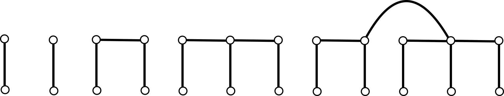
Figure 1: The first five Fibonacci-type trees $T_{k}$ for $1\leq k\leq 5$.

The second family of trees, $\mathcal{A}=\{A_{k}\mid k\geq 1\}$, is defined the following way. Let $A_{1}$ be a single vertex. For $k\geq 2$, $A_{k}=(H\cup J)+uv$ where $H$ and $J$ are two disjoint copies of $A_{k-1}$, and $u$ and $v$ vertices of maximum degree in $H$ and $J$, respectively; see Figure 2.

Thirdly, $\mathcal{B}=\{B_{k}\mid k\geq 1\}$ may be defined in two equivalent ways. For $k\geq 1$, let $u$ be a vertex of maximum degree in $A_{k}$ and let $z$ be a new vertex (namely, $z\notin A_{k}$), then $B_{k}=A_{k}+uz$. It is straightforward to verify that this is equivalent to letting $B_{1}$ be isomorphic to $K_{2}$ and, for $k\geq 2$, letting $B_{k}=(H\cup J)+uv$, where $H$ is a copy of $A_{k-1}$ and $J$ is a copy of $B_{k-1}$ ($u$ and $v$ are vertices of maximum degree in $H$ and $J$, respectively); see Figure 3.

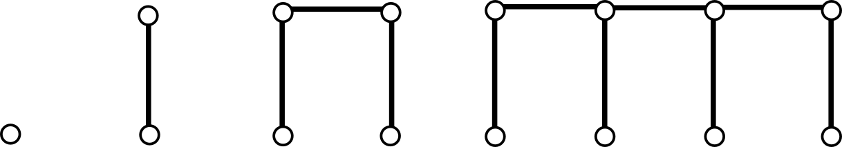
Figure 2: The first four $A_{k}$ trees for $1\leq k\leq 4$.

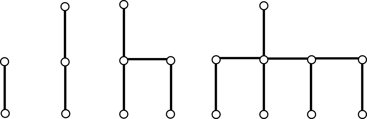
Figure 3: The first four $B_{k}$ trees for $1\leq k\leq 4$.

3 Recursive local amoebas

In [5], different ways of constructing local or global amoebas are presented. Further on, in [9], the authors work with recursive constructions. In particular, a general method to construct families of global amoebas is developed. Using this method, the authors give an alternative proof of the fact that the Fibonacci-type trees from the family $\mathcal{T}$ are global amoebas. We will deal with this family in this section, too, and we will demonstrate that they are local amoebas as well, solving a problem stated in [5]. This will be achieved by means of a general construction that can be used to generate families of local amoebas recursively. By means of this method, it will also be shown that the families $\mathcal{A}$ and $\mathcal{B}$ consist of local amoebas, too.

For a graph $G$ provided with a labeling $\lambda:V(G)\to X$ on its vertices, consider the set $\mathcal{E}_{G}^{i}$ of all permutations associated to edge replacements in $R_{G}$ that fix the label $i\in X$, that is,

$$\mathcal{E}_{G}^{i}=\mathcal{E}_{G}\cap\operatorname{Stab}_{{\rm Fer}(G)}(i).$$

Let ${\rm Fer}^{i}(G)$ be the subgroup of $\operatorname{Stab}_{{\rm Fer}(G)}(i)$ generated by the set $\mathcal{E}_{G}^{i}$. We present the following warm-up lemmas.

Lemma 5.

Let $H$ and $J$ be two vertex disjoint graphs provided with their corresponding disjoint sets of labels $X$ and $Y$. Consider vertices $v_{x}\in V(H)$, $v_{y}\in V(J)$ with labels $x\in X$ and $y\in Y$, respectively, and the graph $G=(H\cup J)+v_{x}v_{y}$ with the inherited set of labels $X\cup Y$. If $\alpha\in\mathcal{E}^{x}_{H}$, then $\alpha\cup{\rm id}_{{\rm Fer}(J)}\in\mathcal{E}^{x}_{G}$.

Proof.

Given $\alpha\in\mathcal{E}^{x}_{H}$, then there is a feasible edge replacement $e\to e^{\prime}\in R_{H}$ such that $\alpha\in{\rm Fer}_{H}(e\to e^{\prime})$. Since $\alpha(x)=x$, the role $v_{x}$ is playing in $H$ is the same as in $H_{\alpha}$, and so the edge replacement $e\to e^{\prime}$ can also be applied on $G$. It follows that

$$G_{\alpha\cup{\rm id}_{{\rm Fer}(J)}}=(H_{\alpha}\cup J)+v_{x}v_{y}\cong(H\cup J)+v_{x}v_{y}=G,$$

implying that $e\to e^{\prime}$ is a feasible edge-replacement in $G$ and $\alpha\cup{\rm id}_{{\rm Fer}(J)}\in\mathcal{E}^{x}_{G}$. ∎

Definition 6 (Stem-symmetric graph).

Let $G$ be a graph and $v\in V(G)$, and let $\lambda:V(G)\to X$ be a labeling of $G$ and $b=\lambda(v)$. We say that $G$ is stem-symmetric with respect to $v$ if ${\rm Fer}^{b}(G)\cong S_{n(G)-1}.$

The following lemma concerns stem-symmetric graphs $G$. It states that $G$ is, in fact, a local amoeba provided we can exhibit a suitable, additional edge-replacement.

Lemma 7.

Let $G$ be a labeled graph that is stem-symmetric with respect to a vertex $v$, whose label is $b$. If

$${\rm Fer}(G)\setminus{\rm Stab}_{G}(b)\neq\emptyset,$$

then $G$ is a local amoeba.

Proof.

Let $X$ be the set of labels of $G$. Recall the following group-theoretic result (see, e.g., [16]). If $x\in X$ and $S\subseteq S_{X\setminus\{x\}}$ is a set of permutations that act transitively on $X\setminus\{x\}$, and if $\varphi\in S_{X}$ with $\varphi(x)\neq x$, then the set $S\cup\{\varphi\}$ generates $S_{X}$. The statement follows by setting $x=b$ and $S={\rm Fer}^{b}(G)$. ∎

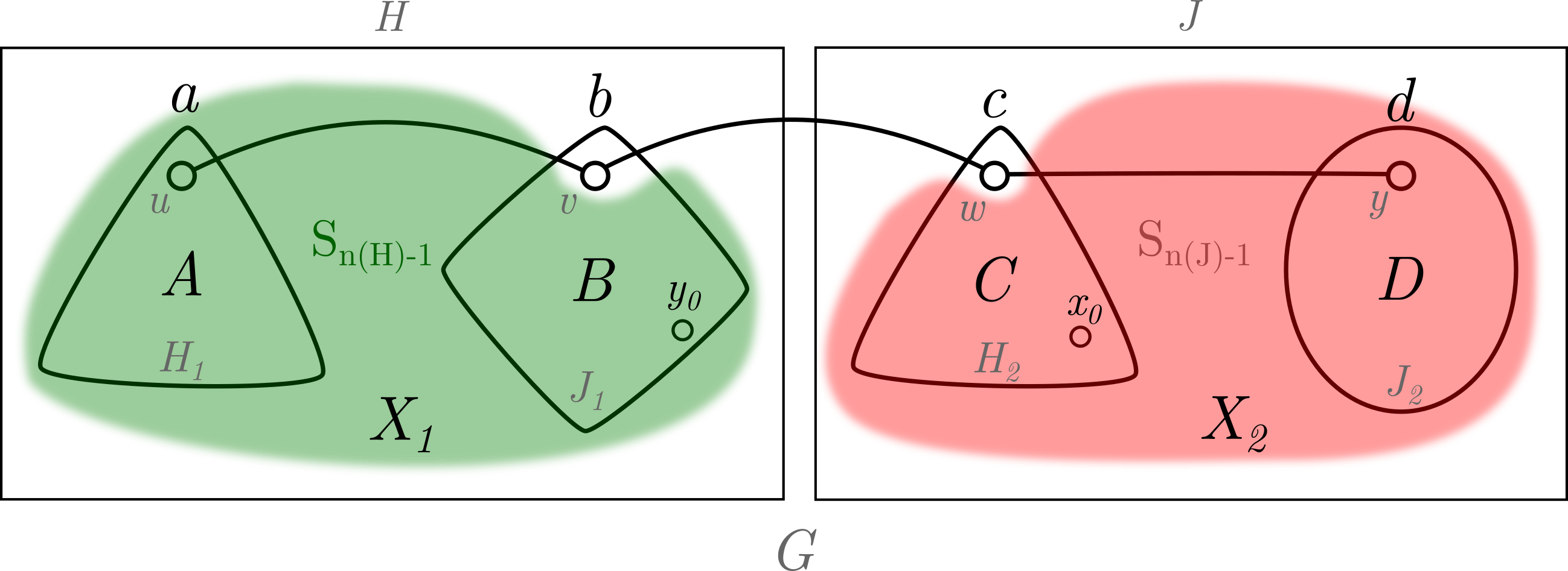
Figure 4: General diagram of Theorem 8.

The theorem below gives a general method by which one can construct local amoebas via a recursion. By Proposition 4, these can be global amoebas, too, if the minimum degree is at most $1$. By means of this theorem, we will be able to prove that the families $\mathcal{T}$, $\mathcal{A}$ and $\mathcal{B}$ consist of local amoebas.

Theorem 8.

Let $H_{1},J_{1},H_{2},J_{2}$ be vertex disjoint graphs provided with the roots $u,v,w,y$, respectively, and such that $H_{1}\cong H_{2}$ and $u$ is similar to $w$. Let $H=(H_{1}\cup J_{1})+uv$ be stem-symmetric with respect to $v$, and $J=(H_{2}\cup J_{2})+wy$ stem-symmetric with respect to $w$. Let $G=(H\cup J)+vw$ be labeled and let $b$ the label on $v$. Then we have the following facts.

1. $G$ is stem-symmetric with respect to $v$.

2. If ${\rm Fer}(G)\setminus{\rm Stab}_{G}(b)\neq\emptyset$, then $G$ is a local amoeba.

3. If ${\rm Fer}(G)\setminus{\rm Stab}_{G}(b)\neq\emptyset$ and $\delta(G)\leq 1$, then $G$ is a global and a local amoeba.

Proof.

(i) We will show first that $G$ is stem-symmetric with respect to $v$. Let $\lambda(u)=a$, $\lambda(v)=b$, $\lambda(w)=c$, and $\lambda(y)=d$. Let $\lambda(V(H_{1}))=A$, $\lambda(V(J_{1}))=B$, $\lambda(V(H_{2}))=C$, and $\lambda(V(J_{2}))=D$, and $X=X_{1}\cup X_{2}$ (clearly, $X_{1}=A\cup B$, and $X_{2}=C\cup D$). See Figure 4 for a general diagram of the proof. We take a fixed element $y_{0}\in B\setminus\{b\}$ and we will prove that $(x\;y_{0})\in{\rm Fer}^{b}(G)$ for every $x\in X\setminus\{b\}$, which would yield that ${\rm Fer}^{b}(G)\cong S_{n(G)-1}$.

To this aim, let $\omega:A\to C$ be the bijection induced by an isomorphism from $H_{1}$ to $H_{2}$ that sends $u$ to $w$. Then we have $\omega(a)=c$. Note that $cd\to ad$ is a feasible edge-replacement of $G$ that yields the permutation $\rho=\prod_{x\in A}(x\;\omega(x))\in{\rm Fer}_{G}(cd\to ad)$ which interchanges the elements in $A$ and $C$ by means of $\omega$ and fixes everything else. In particular, $\rho\in{\rm Fer}^{b}(G)$.

Because ${\rm Fer}^{b}(H)\cong S_{n(H)-1}$, we know that $(x\;y_{0})\in{\rm Fer}^{b}(H)$ for any $x\in(A\cup B)\setminus\{b\}$. Hence, by Lemma 5, $(x\;y_{0})\in{\rm Fer}^{b}(G)$ for any $x\in(A\cup B)\setminus\{b\}$.

Take now any $x\in C$ and consider $\omega^{-1}(x)\in A$. The permutations $\rho$ and $(\omega^{-1}(x)\;y_{0})$ are contained in ${\rm Fer}^{b}(G)$, and thus $(x\;y_{0})=\rho(\omega^{-1}(x)\;y_{0})\rho^{-1}\in{\rm Fer}^{b}(G)$ for any $x\in C$.

Finally, we consider an arbitrary $x\in D$. Take now a fixed $x_{0}\in C\setminus\{c\}$, and observe that $(x\;x_{0})\in{\rm Fer}^{c}(J)\cong S_{n(J)-1}$. By means of Lemma 5, we can even say that $(x\;x_{0})\in{\rm Fer}^{b}(G)$. Since $(x_{0}\;y_{0})\in{\rm Fer}^{b}(G)$, we conclude that $(x\;y_{0})=(x\;x_{0})(x_{0}\;y_{0})(x\;x_{0})\in{\rm Fer}^{b}(G)$.

Hence, we have considered all possibilities for $x\in X\setminus\{b\}$, and we can assert that $(x\;y_{0})\in{\rm Fer}^{b}(G)$ for every $x\in X\setminus\{b\}$. Since such a set of permutations generates the symmetric group on $X\setminus\{b\}$, it follows that ${\rm Fer}^{b}(G)\cong S_{n(G)-1}$, and we are done.

(ii) Since, by (i), $G$ is stem-symmetric with respect to $v$, then, together with the assumption that ${\rm Fer}(G)\setminus{\rm Stab}_{G}(b)\neq\emptyset$, $G$ is a local amoeba by Lemma 7.

(iii) This follows by (ii) and Proposition 4. ∎

Observe that the direct application of this method in a recursive manner results in the construction of a family of quite sparse graphs as we are adding each time a single edge connecting two smaller graphs. However, as complements of local amoebas are again local amoebas [5], it is evident that there are also families of dense local amoebas that can be constructed recursively by these tools, too.

3.1 Application to our case studies

Theorems 9 and 10 use Theorem 8 to prove that our tree constructions are local amoebas and global amoebas.

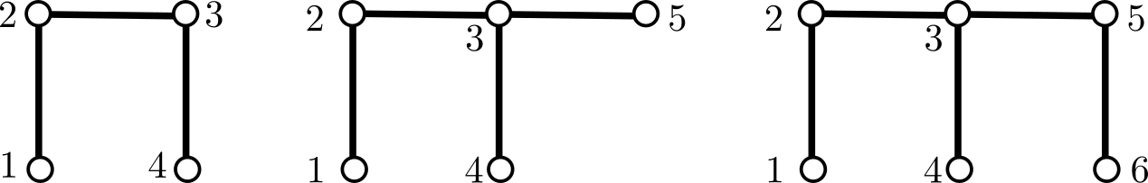
Figure 5: A labeling of $A_{3}=T_{3}$, $B_{3}$ and $T_{4}$.

Theorem 9.

For every $k\geq 1$, the Fibonacci-type tree $T_{k}\in\mathcal{T}$ is both a local and global amoeba.

Proof.

Let $k\geq 1$ and let $X$ be the set of labels for $T_{k}$. Let $v_{i}$ be the vertex of $T_{k}$ with label $i\in X$ and let $v_{b}$ be a vertex of maximum degree in $T_{k}$. We use induction on $k$ and Theorem 8(i) to prove that $T_{k}$ is stem-symmetric with respect to $v_{b}$, then employ Lemma 7 to prove that $T_{k}$ is a local amoeba. For $k=1,2$, the result is trivial. For the cases when $k=3,4$, we proceed to prove that ${\rm Fer}^{b}(T_{3})\cong S_{3}$ and ${\rm Fer}^{b}(T_{4})\cong S_{5}$, and conclude that $T_{3}$ and $T_{4}$ are local amoebas using Lemma 7. Let $T_{3}$ have the labels $\{1,2,3,4\}$ which are arranged as in Figure 5. We use the permutations $(1\,2)\in{\rm Fer}^{3}_{T_{3}}(32\to 31)$ and $(2\,4)\in{\rm Fer}^{3}_{T_{3}}(12\to 14)$ to generate ${\rm Fer}^{3}_{T_{3}}\cong S_{3}$. Since $(1\,2\,3\,4)\in{\rm Fer}_{T_{3}}(43\to 41)\in{\rm Fer}(T_{3})\setminus\operatorname{Stab}_{{\rm Fer}(T_{3})}(3)$, we obtain with Lemma 7 that ${\rm Fer}(T_{3})\cong S_{4}$. For $k=4$, let $\{1,2,3,4,5,6\}$ be the labels of $T_{4}$ arranged as in Figure 5. We use the permutations $(1\,2)\in{\rm Fer}^{3}_{T_{4}}(32\to 31)$, $(2\,4)\in{\rm Fer}^{3}_{T_{4}}(12\to 14)$, $(4\,5)\in{\rm Fer}^{3}_{T_{4}}(65\to 64)$ and $(56)\in{\rm Fer}^{3}_{T_{4}}(35\to 36)$ to generate ${\rm Fer}^{3}_{T_{4}}\cong S_{5}$. Now consider the permutation $(3\,5)(4\,6)\in{\rm Fer}_{T_{4}}(23\to 25)\in{\rm Fer}(T_{4})\setminus\operatorname{Stab}_{{\rm Fer}(T_{4})}(3)$. By Lemma 7, it follows that ${\rm Fer}(T_{4})\cong S_{6}$.

Now let $k\geq 5$ and assume that $T_{i}$ is stem-symmetric with respect to its vertex of maximum degree, for every $i<k$. By construction, $T_{k}$ consists of subtrees $H\cong T_{k-1}$ and $J\cong T_{k-2}$ and an edge $v_{b}v_{c}$ joining their vertices $v_{b}\in V(H)$ and $v_{c}\in V(J)$ of maximum degree. As $H\cong T_{k-1}$, there are subtrees $H_{1}\cong T_{k-3}$ and $J_{1}\cong T_{k-2}$ of $H$, with $v_{a}$ and $v_{b}$ the vertices of maximum degree in $H_{1}$ and $J_{1}$, respectively, such that $H=(H_{1}\cup J_{1})+v_{a}v_{b}$. Similarly, there are subtrees $H_{2}\cong T_{k-3}$ and $J_{2}\cong T_{k-4}$ of $J$, with $v_{c}$ and $v_{d}$ the vertices of maximum degree in $H_{2}$ and $J_{2}$, respectively, such that $J=(H_{2}\cup J_{2})+v_{c}v_{d}$. Clearly, there is an isomorphism from $H_{1}$ to $H_{2}$ that sends $v_{a}$ to $v_{c}$. Moreover, by the induction hypothesis, ${\rm Fer}^{b}(H)\cong S_{n(H)-1}$ and ${\rm Fer}^{c}(J)\cong S_{n(J)-1}$. Hence, we can use Theorem 8(i) to conclude that $T_{k}$ is stem-symmetric with respect to $v_{b}$.

Now consider the feasible edge replacement $ab\to ac$ of $T_{k}$ and take the permutation $\varphi\in{\rm Fer}_{T_{k}}(ab\to ac)$ induced by an isomorphism from $J_{1}\cong T_{k-2}$ to $J\cong T_{k-2}$ that sends $v_{b}$ to $v_{c}$, i.e. we have $\varphi(b)=c\neq b$. It follows by Theorem 8(ii) that $T_{k}$ is a local amoeba.

We conclude, by induction, that every Fibonacci-type tree $T_{k}\in\mathcal{T}$ is a local amoeba for every $k\in\mathbb{Z}^{+}$. ∎

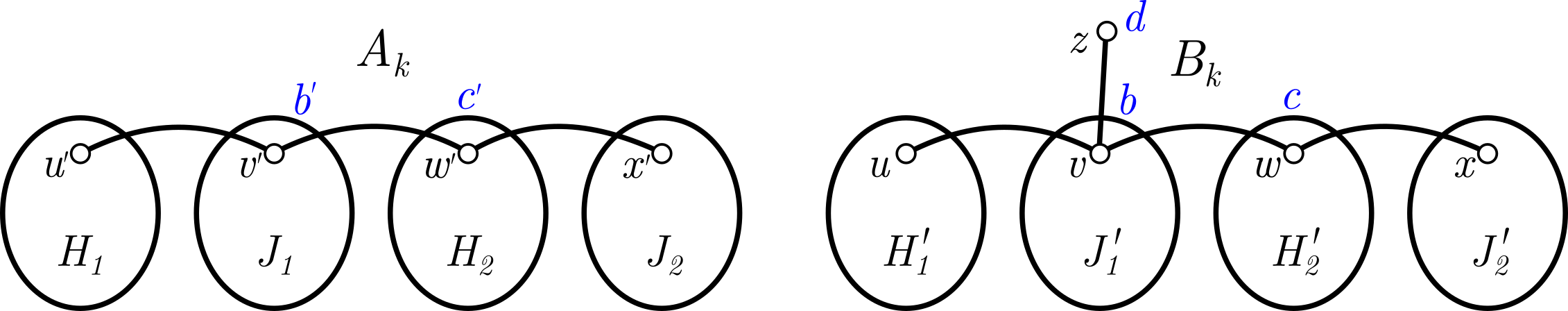
Figure 6: Proof diagrams of Theorem 10.

Theorem 10.

For every $k\geq 1$, $A_{k}\in\mathcal{A}$ and $B_{k}\in\mathcal{B}$ are both local and global amoebas.

Proof.

We proceed in a similar manner as in the proof of Theorem 9. We prove that $A_{k}$ and $B_{k}$ are stem-symmetrical with respect to their vertices of maximum degree by means of Theorem 8(i). Afterwards, we use Theorem 8(ii) to prove that $A_{k}$ and $B_{k}$ are local amoebas. For $k=1,2$, the result is given trivially. For $k=3$, note that $A_{3}\cong T_{3}$, and by Theorem 9, this case is done. Considering $B_{3}$, we use the label set $\{1,2,3,4,5\}$ arranged as in Figure 5. Note that the permutations $(1\,2)\in{\rm Fer}^{3}_{B_{3}}(32\to 32)$, $(2\,4)\in{\rm Fer}^{3}_{B_{3}}(12\to 14)$, and $(2\,5)\in{\rm Fer}^{3}_{B_{3}}(12\to 15)$ generate ${\rm Fer}^{3}(B_{3})\cong S_{4}$. As $(4\,5)\in{\rm Fer}_{B_{3}}(\emptyset\to\emptyset)\setminus\operatorname{Stab}_{{\rm Fer}(T_{3})}(3)$, it follows by Theorem 8(ii) that $B_{3}$ is a local amoeba.

Now let $k\geq 4$ and assume that, for every $j$ with $1\leq j<k$, $A_{j}$ and $B_{j}$ are both stem-symmetric with respect to their vertices of maximum degree as well as local amoebas.

Let $X$ be the set of labels for $A_{k}$, and $Y$ the set of labels for $B_{k}$. Let $b\in X$ and $b^{\prime}\in Y$ be the labels of a vertex of maximum degree in $A_{k}$ and $B_{k}$, respectively. We consider first $A_{k}$. Let $A_{k}=(H\cup J)+vw$, where both $H$ and $J$ are isomorphic to $A_{k-1}$, and $v$ and $w$ are vertices of maximum degree in $H$ and $J$, respectively. Let $v$, which has maximum degree in $A_{k}$, have label $b$. Note that $A_{k}$ can be viewed as four graphs $H_{1}$, $J_{1}$, $H_{2}$, $J_{2}$, each isomorphic to $A_{k-2}$, and $u\in V(H_{1})$, $x\in V(J_{2})$ such that $H=(H_{1}\cup J_{1})+uv$ and $J=(H_{2}\cup J_{2})+wx$ (see Figure 6). Let $c$ be the label of $w$. By the induction hypothesis, ${\rm Fer}^{b}(H)\cong S_{n(H)-1}$, and ${\rm Fer}^{c}(J)\cong S_{n(J)-1}$. Now Theorem 8(i) implies that $A_{k}$ is stem-symmetric with respect to $v$.

The proof that $B_{k}$ is stem-symmetric with respect to a vertex of maximum degree works similarly. Let $B_{k}=(H^{\prime}\cup J^{\prime})+v^{\prime}w^{\prime}$, where $H^{\prime}\cong B_{k-1}$ and $J^{\prime}\cong A_{k-1}$, and $v^{\prime}$ and $w^{\prime}$ are vertices of maximum degree in $H^{\prime}$ and $J^{\prime}$, respectively. Observe first that, by definition, there is a leaf $z$ adjacent to $v^{\prime}$ such that $H^{\prime}-z\cong A_{k-1}$ and that $v^{\prime}$ is the vertex of maximum degree in $B_{k}$. Now consider graphs $H^{\prime}_{1}$, $J^{\prime}_{1}$, $H^{\prime}_{2}$, $J^{\prime}_{2}$ such that $H^{\prime}_{1}$, $H^{\prime}_{2}$ and $J^{\prime}_{2}$ are all isomorphic to $A_{k-2}$ and $J^{\prime}_{1}\cong B_{k-2}$. The vertices $u^{\prime},v^{\prime},w^{\prime},x^{\prime}$ are vertices of maximum degree in $H^{\prime}_{1},J^{\prime}_{1},H^{\prime}_{2}$ and $J^{\prime}_{2}$ respectively. Let $H^{\prime}=(H^{\prime}_{1}\cup J^{\prime}_{1})+u^{\prime}v^{\prime}$ and $J^{\prime}=(H^{\prime}_{2}\cup J^{\prime}_{2})+w^{\prime}x^{\prime}$. Let $c^{\prime}$ and $b^{\prime}$ be the labels of $w^{\prime}$ and $v^{\prime}$, respectively (see Figure 6). By the induction hypothesis, ${\rm Fer}^{b^{\prime}}(H^{\prime})\cong S_{n(H^{\prime})-1}$, and ${\rm Fer}^{c^{\prime}}(J^{\prime})\cong S_{n(J^{\prime})-1}$. Hence, by Theorem 8(i), $B_{k}$ is stem-symmetric with respect to $v^{\prime}$.

Now we show that both $A_{k}$ and $B_{k}$ are local amoebas. Consider a permutation $\varphi\in{\rm Fer}(A_{k})$ that interchanges the labels among the sets $V(H)$ and $V(J)$ induced by an isomorphism that sends $b$ to $c$. Since $\varphi(b)=c\neq b$, it follows by Lemma 7 that $A_{k}$ is a local amoeba. Finally, let $d$ be the label of the leaf $z$ and notice that $db^{\prime}\to dc^{\prime}$ is a feasible edge-replacement in $B_{k}$ that induces the permutation $\varphi^{\prime}\in{\rm Fer}(B_{k})$ which exchanges the elements between $H^{\prime}-z$ and $J^{\prime}$ by means of an isomorphism that takes $v^{\prime}$ to $w^{\prime}$. Hence, $\varphi^{\prime}(b^{\prime})=c^{\prime}\neq b^{\prime}$ and, by Lemma 7, it follows that $B_{k}$ is a local amoeba. ∎

4 Balancing number of global amoebas

In this section, we relate the balancing number of a global amoeba $G$ to the Turán number of a class of graphs $\mathcal{H}_{G}$ which, broadly speaking, contains all subgraphs of $G$ on half its edges; see Theorem 11. This idea was already introduced in [3] with the aim of finding balanced spanning subgraphs but with respect to closed families and, in particular, of local amoebas. Once in the context of Turán theory, we obtain general lower bounds on the balancing number of a global amoeba $G$, based on the size of cuts of $G$. We then apply these results to our case-studies: we determine the balancing number for the smallest cases and, for the larger ones, we provide lower and upper bounds; the latter is based on estimating the Turán number of suitable star forests, contained in the amoeba, on half the edges of the graph under consideration.

For any graph $G$, let

$$\mathcal{H}_{G}=\left\{H:\,H\subset G,\,H\text{ has }\left\lfloor\frac{e(G)}{2}\right\rfloor\text{ edges and no isolated vertices}\right\}$$ (1)

be the class of subgraphs of $G$ that contain half the number of edges of $G$ (rounding down when $e(G)$ is odd). The next theorem establishes the equivalence between the balancing number of a global amoeba $G$ and the Turán number of the class $\mathcal{H}_{G}$. We will make use of the following two well-known facts. By a classical argument of Erdős [10], every graph contains a bipartite subgraph with at least half its edges. Moreover, $\operatorname{ex}(n,H)=o(n^{2})$ for any bipartite graph $H$ (see [11]). Hence, we have that $\operatorname{ex}(n,\mathcal{H}_{G})=o(n^{2})$, as $\mathcal{H}_{G}$ contains at least a bipartite graph.

Theorem 11.

Let $G$ be a global amoeba. Then, for $n$ sufficiently large, $\operatorname{bal}(n,G)=\operatorname{ex}(n,\mathcal{H}_{G})$.

Proof.

Throughout the proof, let $m$ be the number of edges of $G$. We show that $\operatorname{bal}(n,G)$ is an upper bound for $\operatorname{ex}(n,\mathcal{H}_{G})$ and viceversa. Take $n$ large enough such that all arguments in the proof go through.

To show the inequality $\operatorname{ex}(n,\mathcal{H}_{G})\leq\operatorname{bal}(n,G)$, consider a 2-edge-coloring of $K_{n}$ with partition $E(K_{n})=R\cup B$, where $|B|=\operatorname{ex}(n,\mathcal{H}_{G})$ and such that the graph induced by $B$ is free from any member of $\mathcal{H}_{G}$. As $\operatorname{ex}(n,\mathcal{H}_{G})=o(n^{2})$, it follows that $|R|=\binom{n}{2}-|B|\geq|B|$, for $n$ large enough. Since the graph induced by $B$ is $\mathcal{H}_{G}$-free, there is no balanced $G$ in $K_{n}$, implying that $\operatorname{ex}(n,\mathcal{H}_{G})=|B|\leq\operatorname{bal}(n,G)$.

For the other side of the inequality, let $E(K_{n})=R\cup B$ be a 2-edge-coloring of $K_{n}$ satisfying $\min\{|R|,|B|\}>\operatorname{ex}(n,\mathcal{H}_{G})$ (this is possible since $\operatorname{ex}(n,\mathcal{H}_{G})=o(n^{2})$). We proceed to show that the coloring contains a balanced copy of $G$.

Since $|R|>\operatorname{ex}(n,{\mathcal{H}}_{G})$, there is a copy $H_{R}$ of a member from ${\mathcal{H}}_{G}$ contained in the graph induced by $R$. Let $G_{R}\subset K_{n}$ be a copy of $G$ such that $H_{R}\subset G_{R}$ and let $\ell_{R}$ be the number of red edges in $G_{R}$. Similarly, we may consider a blue copy $H_{B}$ of a member from ${\mathcal{H}}_{G}$ contained in the graph induced by $B$. Let $G_{B}\subset K_{n}$ be a copy of $G$ such that $H_{B}\subset G_{B}$ and let $\ell_{B}$ be the number of blue edges in $G_{B}$. By the definition of $\mathcal{H}_{G}$, we have that $\min\{\ell_{R},\ell_{B}\}\geq\lfloor\frac{m}{2}\rfloor$.

Since our aim is to find a balanced copy of $G$ in $R\cup B$, we may assume that neither $G_{R}$ nor $G_{B}$ are balanced, as otherwise we are done; that is, $\{\ell_{R},\ell_{B}\}\cap\{\lfloor\frac{m}{2}\rfloor,\lceil\frac{m}{2}\rceil\}=\emptyset$. Therefore, in what follows, we assume that $\min\{\ell_{R},\ell_{B}\}>\lceil\frac{m}{2}\rceil$.

Since $G$ is a global amoeba, there exists a sequence of subgraphs $G_{0}=G_{R},G_{1},\ldots,G_{k}=G_{B}$ of $K_{n}$ such that, for each $1\leq i\leq k$, $G_{i}$ may be obtained from $G_{i-1}$ by a feasible edge replacement. Let $\ell_{B,i}$ be the number of blue edges in $G_{i}$. Edge replacements may change the number of blue edges in each $G_{i}$ by at most one, that is, $|\ell_{B,i}-\ell_{B,i-1}|\leq 1$. On the other hand, $\ell_{B,0}=m-\ell_{R}<m-\lceil\frac{m}{2}\rceil=\lfloor\frac{m}{2}\rfloor$ and $\ell_{B,k}=\ell_{B}>\lceil\frac{m}{2}\rceil$. Thus, the theorem of the intermediate value implies that there is some $0\leq i\leq k$ for which $\ell_{B,i}\in\{\lfloor\frac{m}{2}\rfloor,\lceil\frac{m}{2}\rceil\}$ and such $G_{i}$ is a balanced copy of $G$. Hence, $\operatorname{ex}(n,\mathcal{H}_{G})$ is an upper bound for $\operatorname{bal}(n,G)$, as desired. Together, these two arguments establish $\operatorname{bal}(n,G)=\operatorname{ex}(n,\mathcal{H}_{G})$. ∎

Moreover, we have the following lower bound on $\operatorname{bal}(n,G)$ for general, global amoebas.

Theorem 12.

Let $G=(V,E)$ be a global amoeba with $k$ vertices, $m$ edges and degree sequence $d_{1}\geq\cdots\geq d_{k}$. For any $\ell\geq 1$ satisfying $\sum_{i=1}^{\ell}d_{i}<\left\lfloor\frac{m}{2}\right\rfloor$, we have $\operatorname{bal}(n,G)\geq\ell(n-\ell)$. In particular,

$$\operatorname{bal}(n,G)\geq\left\lfloor\frac{m-1}{2k+1}\right\rfloor\left(n-\left\lfloor\frac{m-1}{2k+1}\right\rfloor\right).$$

Note that the bound expressed in the theorem is meaningful only when $m\geq 2(k+1)$. The proof of this theorem, which is a consequence of Theorem 11 and the next two lemmas, requires the introduction of the following notation. For a graph $G=(V,E)$ with partition $V=S\cup T$, let

$$e_{G}(S,T)=|\{uv\in E(G):\,u\in S,v\in T\}|;$$ (2)

we say that $e_{G}(S,T)$ is the size of the cut $(S,T)$. For $1\leq\ell\leq|V|$, we define

$$\mathrm{MaxCut}(G,\ell) =\max\{e_{G}(S,V\setminus S):\,S\subset V,|S|\leq\ell\};$$ (3)

$$\ell_{G} =\max\left\{\ell\geq 0:\mathrm{MaxCut}(G,\ell)<\left\lfloor\frac{e(G)}{2}\right\rfloor\right\}.$$ (4)

Observe that $0\leq\ell_{G}<|V|/2$. To see this, note that, as a function of $\ell$, $\mathrm{MaxCut}(G,\ell)$ is non-decreasing and attains its maximum at $\ell=\lfloor\frac{|V|}{2}\rfloor$; while, as mentioned before, every graph $G=(V,E)$ has a cut of size at least $e(G)/2$ [10]; that is,

$$\mathrm{MaxCut}\left(G,\left\lfloor\frac{|V|}{2}\right\rfloor\right)\geq\left\lceil\frac{e(G)}{2}\right\rceil.$$

The following theorem gives a lower bound on $\operatorname{ex}(n,\mathcal{H}_{G})$ in terms of $\ell_{G}$.

Lemma 13.

Let $G=(V,E)$ be a graph. Then, for any $\ell\leq\ell_{G}$,

$$\operatorname{ex}(n,\mathcal{H}_{G})\geq\ell_{G}(n-\ell_{G})\geq\ell(n-\ell).$$

Proof.

For any $n\geq|V|$, using $0\leq\ell_{G}<|V|/2$, we infer that the maximum of $\{\ell(n-\ell):0\leq\ell\leq\ell_{G}\}$ is attained at $\ell=\ell_{G}$. Let us assume $\ell_{G}\geq 1$; otherwise, the statement is trivially satisfied. We claim that the complete bipartite graph $K_{\ell_{G},n-\ell_{G}}$ does not contain any $H\in\mathcal{H}_{G}$ as a subgraph and so $\operatorname{ex}(n,\mathcal{H}_{G})\geq\ell_{G}(n-\ell_{G})$.

Suppose to the contrary that $K_{\ell_{G},n-\ell_{G}}$ contains a copy of some $H\in\mathcal{H}_{G}$, in which case $H$ is bipartite with partition $S\cup R$ and size $\lfloor\frac{m}{2}\rfloor$, where $m=e(G)$. Without loss of generality, we may assume that $|S|\leq\ell_{G}$.

Considering $G$, by definition of $\ell_{G}$ and (4), and assuming $\ell_{G}\geq 1$, we have

$$e_{G}(S,V\setminus S)\leq\mathrm{MaxCut}(G,\ell_{G})<\left\lfloor\frac{m}{2}\right\rfloor.$$

On the other side, since $H$ is bipartite and subgraph of $G$,

$$e_{G}(S,V\setminus S)\geq e_{H}(S,R)=e(H)=\left\lfloor\frac{m}{2}\right\rfloor;$$

which is a contradiction. ∎

In preparation for the proof of Theorem 12, let us consider solutions to the following quadratic inequality.

Lemma 14.

Consider $k,m\geq 1$ such that $(2k+1)^{2}\geq 4(m-1)$ and set $\ell_{0}=\lfloor\frac{m-1}{2k+1}\rfloor$. Any $x\leq\ell_{0}$ satisfies

$$(k+1)x-\frac{x(x+1)}{2}\leq\frac{m-1}{2}.$$

Proof.

Rearranging the terms, we can see that the inequality holds on $(-\infty,x_{-})\cup(x_{+},\infty)$; for $x_{-}$ and $x_{+}$ solutions of the quadratic equation

$$2(k+1)x-x(x+1)-(m-1)=-x^{2}+(2k+1)x-(m-1)=0.$$

The solutions to $x^{2}-bx+c=0$, provided $b^{2}>4c$, are given by

$$x_{\pm}=\frac{b\pm\sqrt{b^{2}-4c}}{2}=\frac{b}{2}\left(1\pm\sqrt{1-\frac{4c}{b^{2}}}\right).$$

The function $f(y)=\sqrt{1-y}-1+y/2$ is concave and its maximum is attained at $f(0)=0$; we infer that, $\sqrt{1-y}\leq 1-y/2$ for $y\in[0,1]$. This implies that

$$x_{-}=\frac{b}{2}\left(1-\sqrt{1-\frac{4c}{b^{2}}}\right)\geq\frac{b}{2}\left(1-\left(1-\frac{2c}{b^{2}}\right)\right)=\frac{c}{b}.$$

Using $b=2k+1$, $c=m-1$ and the definition of $\ell_{0}$, we obtain that $x_{-}\geq\frac{m-1}{2k-1}\geq\ell_{0}$. ∎

Proof of Theorem 12.

Using that the degree sequence $d_{1},d_{2},\ldots,d_{k}$ is listed in non-increasing order, we infer that for any $S\subset V$,

$$e_{G}(S,V\setminus S)\leq\sum_{v\in S}\deg(v)\leq\sum_{i=1}^{|S|}d_{i}.$$

It follows that, if $\ell\geq 1$ satisfies $\sum_{i=1}^{\ell}d_{i}<\left\lfloor\frac{m}{2}\right\rfloor$, then $\ell\leq\ell_{G}$ since

$$\max\{e_{G}(S,V\setminus S):\,S\subset V,|S|\leq\ell\}\leq\sum_{i=1}^{\ell}d_{i}<\left\lfloor\frac{m}{2}\right\rfloor.$$

This, together with Theorem 11 and Lemma 13, implies that $\operatorname{bal}(n,G)=\operatorname{ex}(n,\mathcal{H}_{G})\geq\ell(n-\ell)$.

Finally, we optimize the value of $\ell$ such that $\sum_{i=1}^{\ell}d_{i}<\left\lfloor\frac{m}{2}\right\rfloor$. Since $G$ is a global amoeba, by [5, Proposition 3], we have $d_{i}\leq k+1-i$ for $1\leq i\leq k$, then

$$\sum_{i=1}^{\ell}d_{i}\leq\sum_{i=1}^{\ell}(k+1-i)=(k+1)\ell-\frac{\ell(\ell+1)}{2}.$$

Since we are considering integer variables $k,m$ and $\ell$, the inequality

$$(k+1)x-\frac{x(x+1)}{2}<\left\lfloor\frac{m}{2}\right\rfloor$$

is equivalent to that in the statement of Lemma 14, whose conditions are satisfied since $(2k+1)^{2}>8{k\choose 2}>4m>4(m-1)$. Thus, $\ell_{0}=\lfloor\frac{m-1}{2k+1}\rfloor$ satisfies $\sum_{i=1}^{\ell}d_{i}<\left\lfloor\frac{m}{2}\right\rfloor$ and so $\operatorname{bal}(n,G)=\operatorname{ex}(n,\mathcal{H}_{G})\geq\ell_{0}(n-\ell_{0})$, as desired. ∎

4.1 Applications to our case studies

For a graph $G$ in any of the classes $\mathcal{T},\mathcal{A}$ or $\mathcal{B}$ of global amoebas, we determine the balancing number $\operatorname{bal}(n,G)$ for the smallest cases (see Table 1), and, for the larger ones, we provide upper and lower bounds.

We begin by presenting Theorem 15, which provides a summary of the asymptotic results for each class. We then obtain, in each of the subsequent sections, the proofs for the lower and upper bounds in Theorem 15, and finally, we calculate the balancing numbers corresponding to Table 1 and the proof of Theorem 15.

Theorem 15.

For $n$ sufficiently large,

$$n-1\leq\operatorname{bal}(n,T_{6})\leq 2n-2.$$

For $k\geq 7$,

$$F_{k-4}(n-F_{k-4})\leq\operatorname{bal}(n,T_{k})\leq(F_{k-2}-2)n-{F_{k-2}-1\choose 2}+\delta_{k=7};$$

where $\delta_{k=7}=1$ if $k=7$ and is zero otherwise. And for $k\geq 5$,

$$2^{k-5}(n-2^{k-5})\leq\operatorname{bal}(n,A_{k})\leq\operatorname{bal}(n,B_{k})\leq(2^{k-3}-1)n-{2^{k-3}\choose 2}.$$

Before continuing, we tackle the relation between the balancing number of $A_{k}$ and $B_{k}$ in the following result.

Lemma 16.

For $k\geq 2$, we have that $\operatorname{bal}(n,A_{k})\leq\operatorname{bal}(n,B_{k})$.

Proof.

Since $B_{k}$ has $2^{k-1}$ edges, any balanced copy of $B_{k}$ has $2^{k-2}$ edges of each color. On the other hand, by definiton of $B_{k}$, there exists one leaf $z$ in $B_{k}$ such that $B_{k}-z\cong A_{k}$. This implies that, by removing one (particular) edge from a balanced copy of $B_{k}$, we obtain a balanced copy of $A_{k}$. Therefore, any $2$-edge coloring with a balanced copy of $B_{k}$ contains a balanced copy of $A_{k}$. This implies $\operatorname{bal}(n,A_{k})\leq\operatorname{bal}(n,B_{k})$, as desired. ∎

$G$	$\operatorname{bal}(n,G)$
$T_{1}=T_{2}=A_{2}=B_{1}\cong K_{2}$	0
$T_{3}=A_{3}\cong P_{3}$, $B_{2}\cong P_{2}$, $T_{4}$, $B_{3}$	1
$A_{4}$	3
$T_{5}$, $B_{4}$	6

Table 1: The balancing numbers for the first graphs $G$ in $\mathcal{T}$, $\mathcal{A}$ and $\mathcal{B}$.

4.1.1 Lower bounds

We begin by defining an equivalent expression for the degree sequence of $G$. For a graph $G$, let $V_{i}(G)$ denote the set of vertices of degree $i$ in $G$. The profile of $G$ is given by $\{|V_{i}(G)|;i\geq 0\}$.

Although the general lower bound on Theorem 12 is not meaningful for global amoeba trees, the construction of the classes in our case studies allows us to handle finer bounds for the partial sums $\sum_{i=1}^{\ell}d_{i}$ of the degree sequence of the graphs analysed.

We begin by computing the profile of trees in $\mathcal{T}$ and $\mathcal{A}$. For a non-negative integer $k$, let $F_{k}$ denote the $k$-th Fibonacci number (so that $F_{1}=F_{2}=1$, $F_{3}=2$ and so on).

Lemma 17.

The number of vertices in $T_{k}$ is $2F_{k}$. For $k\geq 4$, the profile of $T_{k}$ is given by

$$|V_{i}(T_{k})|=\begin{cases}F_{k+1-i}&1\leq i\leq 2,\\ F_{k-1-i}&3\leq i\leq k-2,\\ 1&i=k-1,\\ 0&i\geq k.\\ \end{cases}$$

Proof.

Recall that,for $k\geq 4$, $T_{k}$ is obtained from the union of two copies of $T_{k-1}$ and $T_{k-2}$ joined by an edge connecting two vertices of degrees $k-2$ and $k-3$, respectively. In particular,the vertex of maximum degree is unique in $T_{k}$.

We proceed by induction on $k$. The base cases $k\in\{4,5\}$ can be verified directly (see, also, Figure 1). Let $k\geq 6$ and suppose the statement is valid for $k-1$ and $k-2$.

By the induction hypothesis, $T_{k-1}$ and $T_{k-2}$ together contain precisely two vertices of degree $k-3$ and one vertex of degree $k-2$ (two of which are the maximum degree vertices of their corresponding trees). Thus, $T_{k}$ contains precisely one vertex of degree $i$ for $i\in\{k-3,k-2,k-1\}$. This establishes $|V_{i}(k)|=1$ for $k-3\leq i\leq k-1$.

Finally, in constructing $T_{k}$, the vertices of degree $i$ with $1\leq i<k-3$ do not alter their degrees. That is, $V_{i}(T_{k})$ is the disjoint union of $V_{i}(T_{k-1})$ and $V_{i}(T_{k-2})$; which implies the recursive equation

$$|V_{i}(T_{k})|=|V_{i}(T_{k-1})|+|V_{i}(T_{k-2})|;$$

completing the proof for the expression of $|V_{i}(k)|$ in both the cases $i\in\{1,2\}$ and $i\in\{3,\ldots,k-4\}$. ∎

Lemma 18.

The number of vertices in $A_{k}$ is $2^{k-1}$. For $k\geq 2$, the profile of $A_{k}$ is given by

$$|V_{i}(A_{k})|=\begin{cases}2^{k-i-1}&1\leq i\leq k-2,\\ 2&i=k-1,\\ 0&i\geq k.\\ \end{cases}$$

Proof.

Recall that $A_{k}$ is obtained from the union of two copies of $A_{k-1}$ joined by an edge connecting two vertices of maximum degree; each copy containing two such maximal degree vertices which, additionally, are similar.

We proceed by induction on $k$. The base case $k=2$ can be verified directly (see, also, Figure 3). Let $k\geq 3$ and suppose the statement is valid for $k-1$.

In two copies of $A_{k-1}$ there are four vertices of degree $k-2$ which are similar. When we join two of them to form $A_{k}$ we obtain two vertices of degree $k-1$ and are left with two vertices of degree $k-2$. Thus, $|V_{i}(A_{k})|=2$ for $k-2\leq i\leq k-1$. On the other hand, the vertices of degree $i$ with $1\leq i<k-2$ do not alter their degrees. That is $V_{i}(A_{k})$ is the disjoint union of two copies of $V_{i}(A_{k-1})$; which implies, by the induction hypothesis

$$|V_{i}(A_{k})|=2|V_{i}(A_{k-1})|=2^{k-i-1};$$

completing the proof for the cases $1\leq i<k-2$. ∎

We are ready to prove the lower bounds using Theorem 12.

Proposition 19.

For $k\geq 6$, $\operatorname{bal}(n,T_{k})\geq F_{k-4}(n-F_{k-4})$.

Proof.

Recall that $T_{k}$ has $m=2F_{k}-1$ edges and note that $\lfloor\frac{m}{2}\rfloor=F_{k}-1$. Let $d_{1},d_{2},\ldots,d_{2F_{k}}$ be the degree sequence of $T_{k}$. We will show that for $k\geq 6$,

$$\sum_{i=1}^{F_{k-4}}d_{i}\leq F_{k}-2<\left\lfloor\frac{m}{2}\right\rfloor,$$ (5)

from which the statement of the lemma follows by Theorem 12 with $\ell=F_{k-4}$.

First, consider the case $k=6$ separately. In this case, $F_{k-4}=1$, $d_{1}=5$ and $F_{k}-2=6$, so (5) is verified directly.

Now, let $k\geq 7$ and let $V_{>4}(T_{k})$ denote the set of vertices in $T_{k}$ with degree larger than four. By Lemma 17,

$$|V_{>4}(T_{k})|=\sum_{i=5}^{k-1}|V_{i}(T_{k})|=1+\sum_{i=5}^{k-2}F_{k-i-1}=1+\sum_{i=1}^{k-6}F_{i}.$$

It follows from induction on $m\in\mbox{${\mathbb{Z}}$}_{+}$, that $\sum_{i=1}^{m}F_{i}=F_{m+2}-1$ for $m\geq 1$. Hence $|V_{>4}(T_{k})|=F_{k-4}$. Therefore,

$$\sum_{i=1}^{F_{k-4}}d_{i}=\sum_{v\in V_{>4}(T_{k})}\deg_{T_{k}}(v)=\sum_{i=5}^{k-1}i|V_{i}(T_{k})|.$$ (6)

On the other hand, using the recursion of Fibonacci numbers and that $F_{m}\leq 2F_{m-1}$ for $m\geq 3$, we have

$$2F_{k-2}=4F_{k-4}+2F_{k-5}\leq 3F_{k-4}+4F_{k-5}.$$

Consequently, together with Lemma 17, we infer

$$\sum_{i=1}^{4}i|V_{i}(T_{k})|=F_{k}+2F_{k-1}+3F_{k-4}+4F_{k-5}\geq F_{k}+2F_{k-1}+2F_{k-2}=3F_{k}.$$ (7)

Finally, by the hand-shake lemma $\sum_{v}\deg_{T_{k}}(v)=\sum_{i=1}^{k-1}i|V_{i}(T_{k})|=2(2F_{k}-1)$, which together with (6) and (7) yields

$$\sum_{i=1}^{F_{k-4}}d_{i}=\sum_{i=5}^{k-1}i|V_{i}(T_{k})|=4F_{k}-2-\sum_{i=1}^{4}i|V_{i}(T_{k})|\leq F_{k}-2;$$

establishing (5) for $k\geq 7$ and completing the proof. ∎

Similarly, we employ Lemma 18 to provide a lower bound of $\operatorname{bal}(n,A_{k})$.

Proposition 20.

For $k\geq 5$, $\operatorname{bal}(n,A_{k})\geq 2^{k-5}(n-2^{k-5})$.

Proof.

Recall that $A_{k}$ has $m=2^{k-1}-1$ edges and note that $\lfloor\frac{m}{2}\rfloor=2^{k-2}-1$. Let $d_{1},d_{2},\ldots,d_{2^{k-1}}$ be the degree sequence of $A_{k}$. We will show that for $k\geq 5$,

$$\sum_{i=1}^{2^{k-5}}d_{i}\leq 2^{k-2}-2<\left\lfloor\frac{m}{2}\right\rfloor,$$ (8)

from which the statement of the lemma follows by Theorem 12 with $\ell=2^{k-5}$.

First, consider the case $k=5$ separately. In this case, $2^{k-5}=1$, $d_{1}=4$ and $2^{k-2}-2=6$, so (5) is verified directly.

Now, let $k\geq 6$ and let $V_{>4}(A_{k})$ denote the set of vertices in $A_{k}$ with degree larger than four. By Lemma 18, and using the notation within,

$$|V_{>4}(A_{k})|=\sum_{i=5}^{k-1}|V_{i}(A_{k})|=2+\sum_{i=5}^{k-2}2^{k-i-1}=2+\sum_{i=1}^{k-6}2^{i}=2\left(1+\sum_{i=0}^{k-7}2^{i}\right)=2^{k-5}.$$

Hence $|V_{>4}(A_{k})|=2^{k-5}$. Therefore,

$$\sum_{i=1}^{2^{k-5}}d_{i}=\sum_{v\in V_{>4}(A_{k})}\deg_{A_{k}}(v)=\sum_{i=5}^{k-1}i|V_{i}(A_{k})|.$$ (9)

On the other hand, together with Lemma 17, we have

$$\sum_{i=1}^{4}i|V_{i}(A_{k})| =2^{k-2}+2\cdot 2^{k-3}+3\cdot 2^{k-4}+4\cdot 2^{k-5}$$

$$=2^{k-5}(4+6+8+8)=2^{k}-2^{k-2}+2^{k-4};$$ (10)

where in the last equality we use that $4+6+8+8=2^{5}-2^{3}+2$.

Finally, by the hand-shake lemma $\sum_{v}\deg_{A_{k}}(v)=\sum_{i=1}^{k-1}i|V_{i}(A_{k})|=2(2^{k-1}-1)$, which together with (9) and (10) yields

$$\sum_{i=1}^{2^{k-5}}d_{i}=\sum_{i=5}^{k-1}i|V_{i}(A_{k})|=2^{k}-2-\sum_{i=1}^{4}i|V_{i}(A_{k})|=2^{k-2}-2^{k-4}-2\leq 2^{k-2}-2;$$

establishing (8) for $k\geq 6$ and completing the proof. ∎

4.1.2 Upper bounds

Throughout this section, for a graph $G$, let $|G|$ denote the number of edges in $G$. The proof strategy of the next two lemmas is the following. Recall that if $G$ is a global amoeba with $m$ edges, then $\operatorname{bal}(n,G)=\operatorname{ex}(n,\mathcal{H}_{G})$. It then suffices to exhibit $H\in\mathcal{H}_{G}$ (that is, $H\subset G$ with $\lfloor\frac{m}{2}\rfloor$ edges and no isolated vertices) to find, by Theorem 11, the upper bound

$$\operatorname{bal}(n,G)=\operatorname{ex}(n,\mathcal{H}_{G})\leq\operatorname{ex}(H,G).$$

We will thus construct subgraph classes of star forests $\{S_{k},k\geq 5\}$ and $\{R_{k},k\geq 5\}$ such that $S_{k}\in\mathcal{H}_{T_{k}}$ and $R_{k}\in\mathcal{H}_{B_{k}}$. The choice of star forests allows us to apply the following theorem from [14, Theorem 3].

Theorem 21 ([14]).

Let $H=\cup_{i=1}^{k}S^{i}$ be a star forest where $d_{i}$ is the maximum degree of $S^{i}$ and $d_{1}\geq d_{2}\geq\ldots\geq d_{k}$. For $n$ sufficiently large,

$$\operatorname{ex}(n,H)=\max_{1\leq i\leq k}\left\{(i-1)(n-i+1)+{i-1\choose 2}+\left\lfloor\frac{d_{i}-1}{2}(n-i+1)\right\rfloor\right\}.$$

Proposition 22.

For $n$ sufficiently large, $\operatorname{bal}(n,T_{6})\leq 2n-2$ and, for $k\geq 7$

$$\operatorname{bal}(n,T_{k})\leq(F_{k-2}-2)n-{F_{k-2}-1\choose 2}+\delta_{k=7};$$

where $\delta_{k=7}=1$ if $k=7$ and is zero otherwise.

Proof.

We define a class of star forests $\mathcal{S}=\{S_{k}|k\geq 5\}$, together with an auxiliarly class $\mathcal{S}^{+}=\{S^{+}_{k}|k\geq 5\}$ such that $S_{k},S^{+}_{k}\subset T_{k}$ for $k\geq 5$.

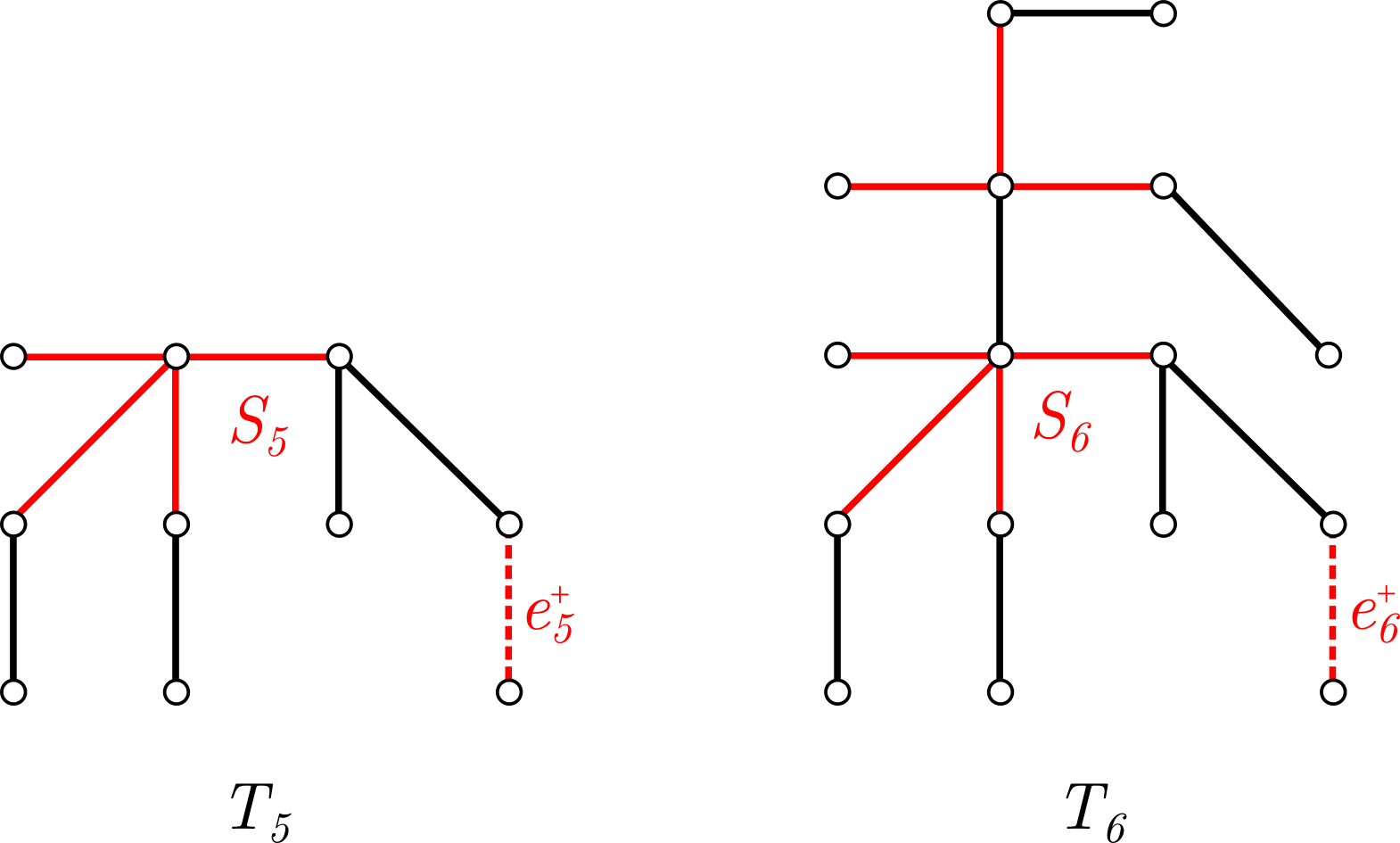
Figure 7: Star forests $S_{5}$ and $S_{6}$ in red. The dotted red edges $e_{5}^{+}$ and $e_{6}^{+}$ define $S_{5}^{+}=S_{5}+e_{5}^{+}$ and $S_{6}^{+}=S_{6}+e_{6}^{+}$, respectively.

First, let $S_{5}$ be a star of degree 4 and let $S_{6}$ be a star forest of one star of degree 4 and one star of degree 3. Then, let $S^{+}_{5}$ and $S^{+}_{6}$ be obtained, respectively, by adding an independent edge to each of $S_{5}$ and $S_{6}$; see Figure 7. For $k\geq 7$, let $S_{k}$ be the disjoint union of two copies of $S_{k-1}$ and $S^{+}_{k-2}$, while defining $S^{+}_{k}$ as the disjoint union of two copies of $S^{+}_{k-1}$ and $S^{+}_{k-2}$. That $S_{k},S^{+}_{k}\subset T_{k}$ is clear from Figure 7 and the construction of $T_{k}$.

Note that $|S^{+}_{5}|=5=F_{5}$, $|S^{+}_{6}|=8=F_{6}$ and $|S_{5}|=4=F_{5}-1$. It can be verified inductively, taking the base cases $S^{+}_{5}$ and $S^{+}_{6}$, the star forest $S^{+}_{k}$ has $F_{k-4}$ stars of maximum degree 4, $F_{k-3}$ stars of maximum degree 3 and $F_{k-3}$ independent edges. Moreover, $|S^{+}_{k}|=|S_{k}|+1=F_{k}$ for all $k\geq 5$; the difference between $S^{+}_{k}$ and $S_{k}$ being an additional, independent edge.

For $1\leq i<F_{k-2}$, let $s_{k,i}$ denote the maximum degree in the $i$-th star of $S_{k}$, the above argument shows that

$$s_{k,i}=\begin{cases}4&1\leq i\leq F_{k-4},\\ 3&F_{k-4}<i\leq F_{k-3},\\ 1&F_{k-3}<i\leq F_{k-2}-1.\end{cases}$$

For $1\leq i<F_{k-2}$, let

$$h_{k}(i,n)=(i-1)(n-i+1)+{i-1\choose 2}+\left\lfloor\frac{s_{k,i}-1}{2}(n-i+1)\right\rfloor.$$

By Theorem 21, $\operatorname{ex}(n,S_{k})=\max_{1\leq i<F_{k-2}}h_{k}(i,n)$. Since the statement in Theorem 21 holds for $n$ sufficiently large, we might as well assume that $n\geq 2F_{k-2}-2$. This implies that $(i-1)(n-i+1)$ is increasing in $i$ and so, as a function of $i$, $h_{k}(i,n)$ is increasing in each of the intervals $[1,F_{k-4}],[F_{k-4}+1,F_{k-3}]$ and $[F_{k-3}+1,F_{n-2}-1]$. In other words,

$$\operatorname{ex}(n,S_{k})=\max\{h_{k}(F_{k-4},n),h_{k}(F_{k-3},n),h_{k}(F_{k-2}-1,n)\}.$$

We then proceed to compare the terms $h_{k}(i,n)$ for $i\in\{F_{k-4},F_{k-3},F_{k-2}-1\}$. We will be concerned, as $n$ is assumed to be large, with the leading term of the following expressions. Letting $\varepsilon_{n}\in\{0,\frac{1}{2}\}$, we have

$$h_{k}(F_{k-4},n) =\frac{2F_{k-4}+1}{2}(n-F_{k-4}+1)+{F_{k-4}-1\choose 2}+\varepsilon_{n}$$

$$=\frac{2F_{k-4}+1}{2}n-\frac{(F_{k-4}+3)(F_{k-4}-1)}{2}+\varepsilon_{n},$$ (11)

$$h_{k}(F_{k-3},n) =F_{k-3}(n-F_{k-3}+1)+{F_{k-3}-1\choose 2}$$

$$=F_{k-3}n-\frac{(F_{k-3}+2)(F_{k-3}-1)}{2},$$ (12)

$$h_{k}(F_{k-2}-1,n) =(F_{k-2}-2)(n-F_{k-2}+2)+{F_{k-2}-2\choose 2}$$

$$=(F_{k-2}-2)n-\frac{(F_{k-2}-2)(F_{k-2}-1)}{2}.$$ (13)

We claim that, together with Theorem 21, these expressions yield

$$\operatorname{ex}(n,S_{k})=\begin{cases}h_{k}(F_{k-3},n)&k=6,\\ h_{k}(F_{k-2}-1,n)+1&k=7,\\ h_{k}(F_{k-2}-1,n)&k\geq 8.\end{cases}$$ (14)

For the case $k\geq 8$, observe that $F_{k-4}+\frac{1}{2}<F_{k-3}<F_{k-2}-2$, implies that (14) holds, for $n$ sufficiently large that the constant terms are negligible compared to $n$. For the cases $k\in\{6,7\}$, the expressions in (11)–(13) above are reduced to

$$h_{6}(F_{2},n) =\frac{3n}{2}+\varepsilon_{n},\qquad\;\,\quad\quad h_{6}(F_{3},n)=2n-2,\qquad h_{6}(F_{4}-1,n)=n-1,$$

$$h_{7}(F_{3},n) =\frac{5(n-1)}{2}+\varepsilon_{n},\qquad h_{7}(F_{4},n)=3n-5,\qquad h_{7}(F_{5}-1,n)=3n-6;$$

which verifies the remaining cases of (14) since $h_{7}(F_{4},n)=h_{7}(F_{5}-1,n)+1$.

Finally, note that the number of edges in $S_{k}$ is

$$\sum_{i=1}^{F_{k-2}-1}d_{i} =4F_{k-4}+3(F_{k-3}-F_{k-4})+(F_{k-2}-F_{k-3}-1)$$

$$=F_{k-4}+2F_{k-3}+F_{k-2}-1$$

$$=F_{k}-1,$$

while $F_{k}$ has $2F_{k}-1$ edges, by Lemma 17. In other words, $S_{k}\in\mathcal{H}_{T_{k}}$; which implies that $\operatorname{bal}(n,T_{k})\leq\operatorname{ex}(n,S_{k})$. Computing the values of (14), using the expressions in (11)-(13), we obtain the desired upper bounds for $\operatorname{bal}(n,k)$ with $n$ sufficiently large. ∎

Proposition 23.

For $k\geq 5$ and $n$ sufficiently large,

$$\operatorname{bal}(n,B_{k})\leq(2^{k-3}-1)n-{2^{k-3}\choose 2}.$$

Proof.

Let $R_{4}\subset B_{4}$ be a star forest comprised of a star of degree 3 and an independent edge; see Figure LABEL:fig:star_forest_Bk. For $k\geq 5$, let $R_{k}$ be the disjoint union of two copies of $R_{k-1}$. Note that, since $A_{4}$ also contains a copy of $R_{4}$, by the construction of $A_{k}$ and $B_{k}$, we may assume that $R_{k}\subset B_{k}$ for all $k\geq 5$.

We can verify inductively that, for all $k\geq 4$, $R_{k}$ contains precisely $2^{k-4}$ stars of degree 3 and $2^{k-4}$ independent edges. Letting $r_{k,i}$ denote the maximum degree in the $i$-th star of $R_{k}$, we conclude that

$$r_{k,i}=\begin{cases}3&1\leq i\leq 2^{k-4},\\ 1&2^{k-4}<i\leq 2^{k-3}.\end{cases}$$

Similarly to the previous proof, we will show that, if $n\geq 2^{k-2}$ (and sufficiently large), $\operatorname{ex}(n,R_{k})=h^{\prime}(2^{k-3},n)$ where,

$$h^{\prime}(i,n)=(i-1)(n-i+1)+{i-1\choose 2}+\left\lfloor\frac{r_{k,i}-1}{2}(n-i+1)\right\rfloor,$$

for $1\leq i\leq 2^{k-3}$. Again, the condition that $n$ is at least as large as twice the number of components in $R_{k}$ guarantees that $h^{\prime}(i,n)$ is increasing in each of the intervals $[1,2^{k-4}]$ and$[2^{k-4}+1,2^{k-3}]$. And so, it suffices to compare the terms

$$h^{\prime}(2^{k-4},n) =2^{k-4}(n-2^{k-4}+1)+{2^{k-4}-1\choose 2},$$

$$h^{\prime}(2^{k-3},n) =(2^{k-3}-1)(n-2^{k-3}+1)+{2^{k-3}\choose 2}.$$

For $k\geq 5$, we have $\frac{3}{2}<2^{k-4}<2^{k-3}-1$. Consequently, for $n$ sufficiently large, and together with Theorem 21, we obtain

$$\operatorname{ex}(n,R_{k})=\max\{h^{\prime}(1,n),h^{\prime}(2^{k-4},n),h^{\prime}(2^{k-3},n)\}=h^{\prime}(2^{k-3},n).$$

This completes the proof as the number of edges in $R_{k}$ is

$$\sum_{i=1}^{2^{k-3}}d_{i}=3\cdot 2^{k-4}+2^{k-4}=2^{k-2}=\left\lfloor\frac{2^{k-1}}{2}\right\rfloor;$$

that is, $R_{k}\in\mathcal{H}_{B_{k}}$ and so

$$\operatorname{bal}(n,B_{k})\leq\operatorname{ex}(n,R_{k}) =(2^{k-3}-1)(n-2^{k-3}+1)+{2^{k-3}-1\choose 2}$$

$$=(2^{k-3}-1)n-{2^{k-3}\choose 2}.$$

∎

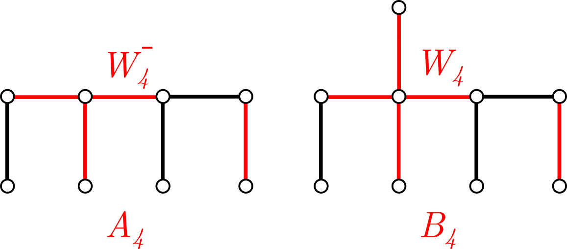
Figure 8: Star forests $W^{-}_{4}$ and $W_{4}$ in red; $W^{-}_{4}$ is contained in both $A_{4}$ and $B_{4}$.

The proof of Theorem 15 is a direct consequence of Propositions 19 and 22 for the class $\mathcal{T}$, and Lemma 16 and Propositions 20 and 23 for the classes $\mathcal{A}$ and $\mathcal{B}$.

4.1.3 Balancing numbers of the small cases

Recall that Theorem 11 provides an equivalence between the balancing number of a global amoeba $G$ and the extremal Turán of $\mathcal{H}_{G}$ as defined in (1). This is straightforward to explore for the first few elements of our case study classes $\mathcal{T},\mathcal{A}$ and $\mathcal{B}$; which coincidentally, by Theorem 15, are the unique elements of such classes with a constant balancing number.

Within the proof of the next lemma, we make use of the following facts.

Claim: For a connected graph $C$ with $m$ edges,

1. if $m\geq 1$, then $C$ contains an edge, $K_{2}$;

2. if $m\geq 2$, then $C$ contains a path on two edges, $P_{2}$;

3. if $m\geq 3$, then $C$ is either a triangle or, contains either a star $S_{3}$ or a copy of $P_{m}$.

Lemma 24.

We have the following balancing numbers.

• $\operatorname{bal}(n,A_{2})=0$, $\operatorname{bal}(n,A_{3})=1$ and $\operatorname{bal}(n,A_{4})=3$,

• $\operatorname{bal}(n,B_{1})=0$, $\operatorname{bal}(n,B_{2})=\operatorname{bal}(n,B_{3})=1$ and $\operatorname{bal}(n,B_{4})=6$,

• $\operatorname{bal}(n,T_{1})=\operatorname{bal}(n,T_{2})=0$, $\operatorname{bal}(n,T_{3})=\operatorname{bal}(n,T_{4})=1$ and $\operatorname{bal}(n,T_{5})=6.$

Proof.

The first few elements in $\mathcal{T},\mathcal{A}$ and $\mathcal{B}$ are paths (or isolated vertices) and their balancing numbers are straightforward to obtain. For the rest of the cases, $T_{4}$ (which equals $B_{3}$), $A_{4},T_{5}$ and $B_{4}$, we make use of the equivalence in Theorem 11.

Observe that $\mathcal{H}_{T_{4}}=\mathcal{H}_{B_{3}}$, $\mathcal{H}_{A_{4}}$ and $\mathcal{H}_{B_{4}}=\mathcal{H}_{T_{5}}$ consist of all forests on two, three and four edges, respectively; see Figures 9 and 10. In particular, $\mathcal{H}_{T_{4}}=\mathcal{H}_{B_{3}}$ consists of exactly two non-isomorphic graphs: $2K_{2}$ and $P_{2}$. Therefore $\operatorname{ex}(n,\mathcal{H}_{T_{4}})=\operatorname{ex}(n,\mathcal{H}_{B_{3}})=1$, and by Theorem 11 we have $\operatorname{bal}(n,T_{4})=\operatorname{bal}(n,B_{3})=1$.

Consider $\mathcal{H}_{A_{4}}$. To prove that $\operatorname{ex}(n,\mathcal{H}_{A_{4}})\geq 3$, it suffices to consider a triangle as the extremal graph. To prove that $\operatorname{ex}(n,\mathcal{H}_{A_{4}})\leq 3$, let $G$ be a graph on 4 edges with no isolated vertices and connected components $C_{1},\dots,C_{\ell}$ which are in decreasing order in terms of the number of edges. In each of the distinct cases below, we find some $H_{i}\in\mathcal{H}_{A_{4}}$.

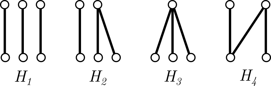
Figure 9: Family $\mathcal{H}_{A_{4}}$.

When $\ell\geq 3$, we may take one edge from each of three components to find $3K_{2}\cong H_{1}\subseteq G$. For the case $\ell=2$, it suffices to apply Claim (ii) to $C_{1}$ and Claim (i) to $C_{2}$ to produce the subgraph $H_{2}$, isomorphic to $P_{2}\cup K_{2}$. Lastly, if $\ell=1$ ($G$ is connected), we consider the maximum degree $\Delta$. If $\Delta\geq 3$, then $G$ contains a copy of the star $H_{3}$; on the other hand, if $\Delta=2$, since $G$ is connected we may find a path on three edges; that is $H_{4}\cong P_{3}$ as a subgraph of $G$. Having covered all possible cases for the components $C_{1},\ldots,C_{\ell}$ we infer $\operatorname{ex}(n,\mathcal{H}_{A_{4}})=3$, and by Theorem 11, $\operatorname{bal}(n,A_{4})=3$.

Finally, consider $\mathcal{H}_{T_{5}}$. We proceed to prove that $\operatorname{ex}(n,\mathcal{H}_{T_{5}})=6$. To prove the lower bound, it suffices to take a complete graph on four vertices as the extremal graph in both cases. To prove the upper bound, let $G$ be a graph on 7 edges with no isolated vertices and connected components $C_{1},\dots,C_{\ell}$ ordered decreasing in size. In each of the distinct cases below, we find some $F_{i}\in\mathcal{H}_{T_{5}}$.

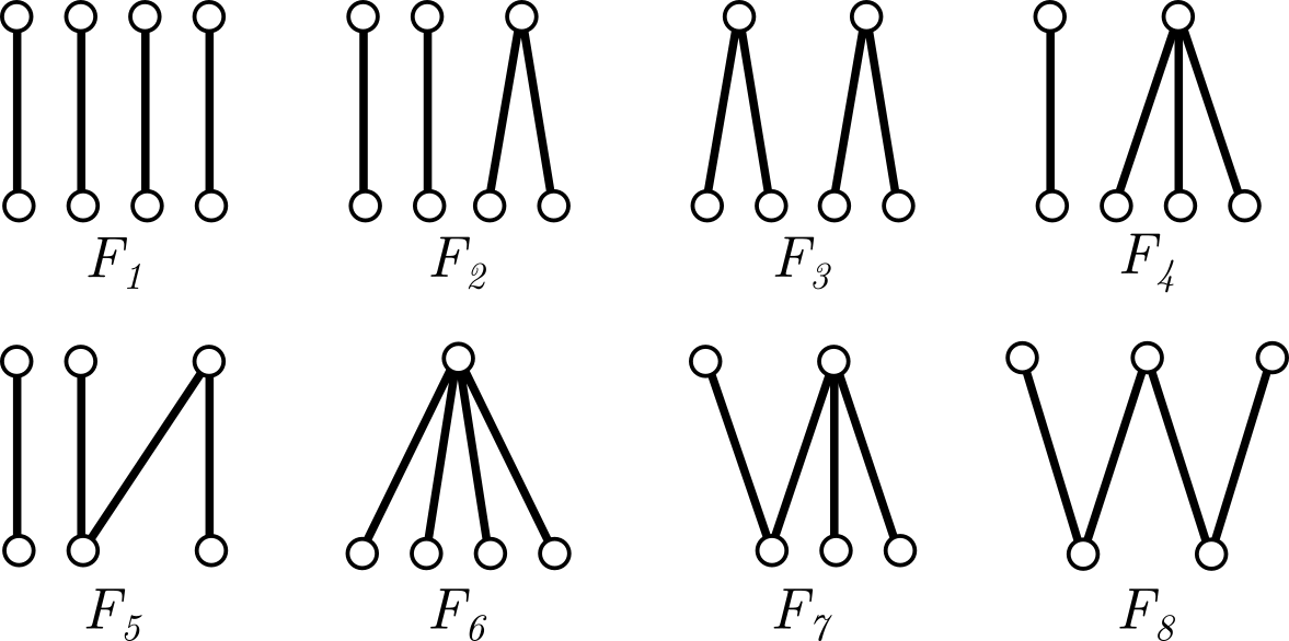
Figure 10: Family $\mathcal{H}_{T_{5}}=\mathcal{H}_{B_{4}}$.

Suppose that $\ell\geq 4$; we may take one edge from each of three components to find $3K_{2}\cong H_{1}\subseteq G$. If $\ell=3$, then $e(C_{1})\geq 2$ and so $C_{1}$ contains a copy of $P_{2}$. We then may take one edge from $C_{2}$ and $C_{3}$ to find a subgraph $F_{2}$ isomorphic to $P_{2}\cup K_{2}\cup K_{2}$. In the case when $\ell=2$ both $C_{1}$ and $C_{2}$ have at least two edges each, we can find, by means of two uses of Claim (ii), that $F_{3}\subseteq G$ which is isomorphic to two disjoint 2-paths. If, on the other hand, $C_{1}$ has 6 edges and $C_{2}$ has one, by Claim (iii), we can find $F_{4}\cong S_{3}\cup K_{2}$ or $F_{5}\cong P_{3}\cup K_{2}$. Finally, if $\ell=1$, then $G$ is connected and we consider the maximum degree $\Delta$. First, suppose that $\Delta\geq 4$, then $G$ contains a star $F_{6}\cong S_{4}$. Now consider $\Delta=3$ and let $v$ be a vertex of maximum degree. We claim there is a vertex $w$ such that $d(v,w)=2$. Otherwise, all vertices would be adjacent to $v$, but $\deg(v)=\Delta=3$, so $G$ could not have 7 edges. We conclude the existence of $F_{7}\subseteq G$, a star $S_{3}$ with an edge joined to $w$. If $\Delta=2$, then Claim (iii) yields $F_{8}\cong P_{4}\subseteq G$. Therefore, $\operatorname{ex}(n,\mathcal{H}_{B_{4}})=\operatorname{ex}(n,\mathcal{H}_{T_{5}})=6$, and by Theorem 11 we obtain that $\operatorname{bal}(n,T_{5})=\operatorname{bal}(n,B_{4})=6$. ∎

5 Algorithms and implementation

In this section, we present an algorithm based on Theorem 9 that finds, given any arbitrary permutation $p$ on the vertices of $T_{k}$, a corresponding sequence of feasible edge replacements in time $\Theta(|V(T_{k})|^{2})$. Similar algorithms exist for any of the local amoebas constructed in Section 3.

We begin by defining a class of objects called Fer with two attributes: a sequence of feasible edge replacements and its corresponding permutation. We denote the length of the sequence of the object fer by len(fer). The product of two Fer objects multiplies their permutations and concatenates the edge replacements, updating the labels. In this implementation, products of permutations (denoted by concatenation) and products of Fer objects (denoted by $*$) are written left-to-right, in contrast with the rest of the paper. This is to be consistent with Python’s symbolic math library SymPy. It is enough to produce a hash map that links every permutation in a generating set of the symmetric group to a Fer object to find the Fer object of any permutation.

We assume that the hash maps for $k=1,2,3,4$, i.e. the recursive basis of Theorem 9, have been previously computed and include all of the permutations (not just the generators). Achieving this is out of the scope of this paper, but our implementation [15] performs this step as well.

We describe each step of the main program, as well as each case of the function RecursiveFer.

1. Write the permutation as a product of disjoint cycles $C=(a_{0},a_{1},\dots,a_{m})$. Then, $C=(y_{0},a_{0})(y_{0},a_{1})\cdots(y_{0},a_{m})(y_{0},a_{0})$. This step yields a list of transpositions of the form $(y_{0},x)$ where $x$ is moved by the permutation and whose product is the permutation.

2. We use RecursiveFer to find a Fer object for each transposition. It is enough to pass the primitive $x$ as an argument, and this makes it easier to employ memoization; otherwise, we would need to either encode permutations into immutable objects or defining an object hashing. Python’s functools library contains a memoization decorator called @cache which saves the values of the function in an internal hash map. Alternatively, we can achieve the same result by updating hashMap and checking, at the beginning of each iteration, if the arguments have been passed before. This costs $O(1)$ time and drastically shortens the execution. For instance, in our experiments, computing RecursiveFer($(0\ 1)\cdots(464\ 465)$, $k=13$) without memoization takes about 293% longer than with it. We describe each case here, however details can be found in the proof of Theorem 9.

   • Notice that $(y_{0},x)=\varphi^{-1}(y_{0},\varphi^{-1}(x))\varphi$, and that we can find a Fer object for $(\varphi^{-1}(x),y_{0})$ since $\varphi^{-1}(x)\in B$.

   • Since $A\cup B\cong T_{k-1}$, a simple recursion works for this case.

   • We may pick $x_{0}$ as any neighbor of $c$. In the labeling of Theorem 9, $x_{0}=c+1$ works, for example. Observe that $(y_{0},x)=\rho^{-1}(y_{0},\rho^{-1}(x))\rho$, and that we can find a Fer object for $(\rho^{-1}(x),y_{0})$, because $\rho^{-1}(x)\in A$.

   • Notice that $(y_{0},x)=(y_{0},x_{0})(x,x_{0})(y_{0},x_{0})$. We can find a Fer for $(y_{0},x_{0})$ since $x_{0}\in C$ in the same $k$. And we can find one for $(x,x_{0})$ because $x-c\in B_{k}\cap(C_{k-2}\cup D_{k-2})$. After finding the Fer object, we need to shift back the labels to $T_{k}$ by adding $c$ to all of them.

3. We get a Fer object corresponding to the permutation obtained from multiplying (using the product $*$) all elements in transpositions. Namely, a sought Fer object for the given permutation.

1

2

@cache

  // Memoization decorator for dynamic execution of recursive function

3 Function RecursiveFer($x$, $k$):

4       if $k\leq 4$ then

            return hashMap[$(y_{0},x)$]

              // Fer is known for the base cases.

5            

6      

7      Let $a,b,c,d$ be the roots of $T_{k}$ and $A,B,C,D$ the sets as defined in Theorem 9.

8      if $x=b$ then

9             $\varphi=$ isomorphism $B\to C\cup D$ with Fer object $(ab\to ac)$

10             return $\varphi*$RecursiveFer($\varphi^{-1}(x)$, $k$)$*\varphi$

      /* If the program gets to this line, it must mean that $x\neq b$. */

11      

12      if $x\in A\cup B$ then

13            return RecursiveFer($x$, $k-1$)

14      

15      if $x\in C$ then

16             $\rho=$ isomorphism $A\to C$ with Fer object $(cd\to ad)$

17             return $\rho*$RecursiveFer($\rho^{-1}(x)$, $k$)$*\rho$

18      if $x\in D$ then

19             $x_{0}=$ a neighbor of the root $c$ in $C$.

20             $y_{0}x_{0}$ = RecursiveFer($x_{0}$, $k$)

             $xx_{0}$ = RecursiveFer($x-c$, $k-2$)$+c$

              // $+c$ shifts all labels in the object by $c$ units.

21             return $y_{0}x_{0}*xx_{0}*y_{0}x_{0}$

22      

23

Input: $k$, permutation

hashMap = $\{\text{generators for }k\leq 4\}$

  // Save known Fer objects in a hash map.

24

/* Step 1: Factor permutation into transpositions of the form $(y_{0},x)$. */

transpositions = $\varnothing$

  // Initialize empty list.

25 for $C$ cycle of permutation do

26       for $x\in C$ do

            transpositions.add($y_{0}$,$x$)

              // Add elements to list.

27            

      transpositions.add($y_{0}$,$a_{0}$)

        // $a_{0}$ is the first element of $C$.

28      

29

/* Step 2: Find Fer for each transposition. */

30 for $x$ where $(y_{0},x)$ in transpositions do

31       xFer = RecursiveFer($x$, $k$)

       hashMap[$(y_{0},x)$] = xFer

        // Save result in a hash map.

32      

/* Step 3: Multiply hashMap values to get a Fer for permutation. */

$$\text{fer}=\prod_{(y_{0},x)\in\text{transpositions}}\text{hashMap}[(y_{0},x)]$$

Output: fer

Algorithm 1 Factoring a permutation into a list of feasible edge replacements Fer in $T_{k}$.

For the analysis, we care about expressing the time and space complexity in terms of the number of vertices of $T_{k}$, namely $n(k)=2F_{k}$. During Step 1, the maximum number of transpositions any permutation gets factored in is achieved by conjugates of $(0\ 1)(2\ 3)(4\ 5)\cdots(n(k)-2\ n(k)-1)$. Thus, with memoization and fixed $k$, the function RecursiveFer($x$,$k$) gets called at most $n(k)-1$ times. It remains to study how long it takes to find a Fer object for each transposition.

Fix $k>5$. We may compute, beforehand and for all $q\leq k$, the isomorphisms $\varphi$ and $\rho$, the roots $a,b,c,d$ and the sets $A,B,C,D$ of $T_{q}$. With memoization, $2F_{k}$ may be computed in time $O(k)$. The roots can be found in constant time since all is needed are smaller values $F_{q}$. The algorithm only needs the sets to evaluate Booleans of the form $x\in S$. But, picking the appropriate labeling of $T_{k}$, this would only require comparing $x$ to the endpoints of $S$, namely two of the roots. Hence, this can still be achieved in constant time. The isomorphisms can be generated in linear time and then applied in linear time.

Multiplying two Fer objects takes linear time in the length of the right-most sequence of replacements, since the labels must be updated one by one. Call this time $m(\ell)$, so that $m(\ell)=O(\ell)$. The product of the permutations takes constant time.

Remark 25.

It is possible to find Fer objects for all transpositions of the form $(y_{0},x)$ in $T_{k}$, when $k\leq 4$, of length 3 or less.

Thus, in general, we have the following result.

Lemma 26.

Let $\ell(k)$ be the maximum length of a Fer object produced by RecursiveFer($x$, $k$). Then, for $k\geq 3$,

$$\ell(k)\leq k^{2}-3k+3.$$

Proof.

Write $R=$ RecursiveFer, for short. First, we argue that, for $k\geq 4$, $\operatorname{len}R(x_{0}^{(k)},k)\leq 2k+5$ by induction on $k$. For simplicity, let us pick $x_{0}^{(k)}=c_{k}+1$, which corresponds to the labeling we give in Theorem 9. We have that $\operatorname{len}R(c_{4}+1,4)\leq 3$ by Remark 25. Now suppose that $k>4$. According to case $x\in C$ in the algorithm and the fact that $\rho_{k}^{-1}(c_{k}+1)=a_{k}+1=c_{k-1}+1$ (see Figure 4),

$$R(c_{k}+1,k)=\rho_{k}*R(\rho_{k}^{-1}(c_{k}+1),k-1)*\rho_{k}=\rho_{k}*R(c_{k-1}+1,k-1)*\rho_{k}$$

has length at most $2(k-5)+3+2=2(k-4)+3$, as desired.

Next, consider the recurrence $r(k)=4k-10+r(k-2)$, $r(3)=r(4)=3$. Inductively, $r(k)-r(k-1)\geq 4$ for all $k\geq 5$. Indeed, since $r(5)=20-10+r(3)=13$, we have that $r(5)-r(4)=13-3=10\geq 4$ and $r(6)-r(5)=4\cdot 6-10+3-13=4$. Then,

$$r(k)-r(k-1) =4k-10+r(k-2)-4(k-1)+10-r(k-3)$$

$$=r(k-2)-r(k-3)+4>4.$$

Finally, we use induction on $k$ to prove that $\ell(k)\leq r(k)$ for all $k\geq 3$. By Remark 25, we know that $\ell(3)=\ell(4)=3=r(3)=r(4)$.

Let us study the computation of $R(x,k)$. Following Algorithm 1. In the case when $x\in A\cup B\setminus\{b\}$, $\operatorname{len}R(x,k)=\operatorname{len}R(x,k-1)\leq\ell(k-1)\leq r(k-1)<r(k)$. If $x\in C\cup\{b\}$, since $\varphi$ and $\rho$ consist of a single edge-replacement, $\operatorname{len}R(x,k)\leq\ell(k-1)+2\leq r(k-1)+2<r(k)$. Finally, if $x\in D$, we need to do two sub-computations: $R(c_{k}+1,k)$ and $R(x-c_{k},k-2)$.

Using the first claim of this proof,

$$\operatorname{len}R(x,k)\leq 2\operatorname{len}R(c_{k}+1,k)+\ell(k-2)\leq 2(2k+5)+r(k-2)=r(k).$$

This concludes the induction.

Now, it remains to find an explicit formula for $r(k)$. But this a linear recurrence with constant coefficients of order 1, which is easily solved using the theory of eigenvectors. Namely, $r(k)=k^{2}-3k+1-2(-1)^{k}\leq k^{2}-3k+3$, from where the result follows. ∎

Theorem 27.

The running time of Algorithm 1 is $\Theta(n^{2})$ and the space complexity is $O((k-4)(n(k)-1))=O(n\log n)$.

Proof.

Let $t(x,k)$ be the time needed to compute RecursiveFer($x$, $k$). By assumption, $t(x,k)=O(1)$ for all $x$ and for all $k\leq 4$. Suppose that $c$ is the maximum of such constants. Inductively,

$$t(x,k)=\begin{cases}t(\varphi^{-1}(x),k-1)+m(\ell(k-1)),&x=b\\ t(x,k-1),&x\in A\cup B\setminus\{b\}\\ t(\rho^{-1}(x),k-1)+m(\ell(k-1)),&x\in C\\ t(\rho^{-1}(x_{0}),k-1)+t(x-c,k-2)+m(\ell(k-1))+m(\ell(k-2)),&x\in D.\end{cases}$$

If $t(k)$ is the worst time of all values of $x$, then, succinctly,

$$t(k)=t(k-1)+t(k-2)+O(k^{2})=cF_{k}+O(k^{2})=O(\phi^{k}),$$

where $\phi$ is the golden ratio.

In terms of $n$, $t(k)\approx\frac{cn}{2}$, which joined with our previous observations, we have that the time complexity is $O(n^{2})$.

The best case is when the input is a transposition $(y_{0},x)$ with $x\in A_{4}\setminus\{y_{0}\}$. Since the sequence of sets $A_{k}$ is increasing, this means RecursiveFer$(x,k)$ will positively evaluate $x\in A_{q}$ $k-4$ times and then look up the generator in the hash map of $T_{4}$ in constant time to produce an output of length at most 3. In other words, the algorithm takes linear time (and linear space complexity too) in $k$ for this input, or $O(\log n)$. However, if the input is a conjugate of $(0\ 1)(2\ 3)(4\ 5)\cdots(2F_{k}-2\ 2F_{k}-1)$, the algorithm will evaluate RecursiveFer$(x,k)$ once for all $x$. ∎

To close off, we point out that since the proof of Theorem 9 uses transpositions to generate the symmetric groups, an algorithm that factors $(0\ 1)(2\ 3)(4\ 5)\cdots(2F_{k}-2\ 2F_{k}-1)$ more efficiently than Algorithm 1 likely uses a very different approach (see open questions of Section 6).

Some technical improvements may stem from the following two observations.

• A Fer sequence can be simplified in some cases. For instance, the sequence $(1\ 2\to 0\ 1)(2\ 3\to 1\ 2)$ is equivalent to $(2\ 3\to 0\ 1)$. The algorithm produces long sequences, and thus simplification may become indispensable for practical purposes. A simple version of this is implemented in [15].

• Ideally, automorphisms should correspond to the trivial edge replacement $(\emptyset\to\emptyset)$, but our algorithm does not account for this. It is not immediately evident when a product of generators is an automorphism.

6 Conclusion and open problems

We finish this paper by stating some open problems that are left for future research concerning the topic of amoebas. It would be interesting to explore if there is a way to characterize global and local amoebas via constructions. However, this problem seems to be quite ambitious. The problems we state here concern the construction of amoebas that try to go in that direction.

1. Generalize the construction of Theorem 8.

2. Look for other general ways of constructing global or local amoebas.

3. Characterize local amoeba trees.

4. Characterize global amoeba trees.

5. Study the balancing number of other amoeba families.

References

[1] Aho, A. V., Hopcroft, J. Ullman, J. D. (1974), The Design and Analysis of Computer Algorithms, Reading, MA: Addison-Wesley, p. 84–86.
[2] Babai, L. (2015), Graph Isomorphism in Quasipolynomial Time, arXiv:1512.03547.
[3] Caro, Y., Hansberg, A., Lauri, J., Zarb, C. (2022), On zero-sum spanning trees and zero-sum connectivity, Electron. J. Combin. 29, no.1, Paper No. 1.9, 24 pp.
[4] Caro, Y., Hansberg, A., Montejano, A. (2021). Unavoidable chromatic patterns in 2-colorings of the complete graph. Journal of Graph Theory, 97(1), 123-147.
[5] Caro, Y., Hansberg, A., Montejano, A. (2023). Graphs isomorphisms under edge-replacements and the family of amoebas. Electronic Journal of Combinatorics 30(3) P3.9
[6] Caro, Y., Lauri, J., Zarb, C. (2022). On small balanceable, strongly-balanceable and omnitonal graphs. Discussiones Mathematicae: Graph Theory, 42(4).
[7] Dona, D., Bajpai, J., Helfgott, H. A. (2017). Graph isomorphisms in quasi-polynomial time, arXiv:1710.04574
[8] Espinosa Hernández, J. (2020) Gráficas inevitables en 2-coloraciones de la gráfica completa: el caso de las amoebas, Tesis de licenciatura, Facultad de Ciencias, UNAM.
[9] Hansberg, A., Montejano, A., Caro, Y. (2021). Recursive constructions of amoebas. Procedia Computer Science, 195, 257-265.
[10] Erdős, P. (1965). On some extremal problems in graph theory. Israel Journal of Mathematics, 3(2), 113-6.
[11] Füredi, Z., Simonovits, M. (2013). The history of degenerate (bipartite) extremal graph problems. Bolyai Soc. Math. Stud., 25, János Bolyai Mathematical Society, Budapest, 169-264.
[12] Kelly, P. J. (1957), A congruence theorem for trees, Pacific Journal of Mathematics, 7: 961–968.
[13] Laffitte, M. E. G., González-Martínez, J. R., & Montejano, A. (2023). On the detection of local and global amoebas: theoretical insights and practical algorithms (Brief Announcement). Procedia Computer Science, 223, 376-378.
[14] Lidicky, B., Liu, H., Palmer, C. (2013). On the Turán number of forests. Electronic Journal of Combinatorics 20(2) P62.
[15] Matos Wiederhold, T. (2023). Feasible Edge Replacements - Class and Algorithms (Version 1.0.0) [Computer software]. https://github.com/tonamatos/Feasible-Edge-Replacements
[16] Rotman, J. J. (2012). An introduction to the theory of groups (Vol. 148). Springer Science & Business Media.