SatCLIP: Global, General-Purpose Location Embeddings with Satellite Imagery

Abstract

Geographic location is essential for modeling tasks in fields ranging from ecology to epidemiology to the Earth system sciences. However, extracting relevant and meaningful characteristics of a location can be challenging, often entailing expensive data fusion or data distillation from global imagery datasets. To address this challenge, we introduce Satellite Contrastive Location-Image Pretraining (SatCLIP), a global, general-purpose geographic location encoder that learns an implicit representation of locations from openly available satellite imagery. Trained location encoders provide vector embeddings summarizing the characteristics of any given location for convenient usage in diverse downstream tasks. We show that SatCLIP embeddings, pretrained on globally sampled multi-spectral Sentinel-2 satellite data, can be used in various predictive tasks that depend on location information but not necessarily satellite imagery, including temperature prediction, animal recognition in imagery, and population density estimation. Across tasks, SatCLIP embeddings consistently outperform embeddings from existing pretrained location encoders, ranging from models trained on natural images to models trained on semantic context. SatCLIP embeddings also help to improve geographic generalization. This demonstrates the potential of general-purpose location encoders and opens the door to learning meaningful representations of our planet from the vast, varied, and largely untapped modalities of geospatial data.

1 Introduction

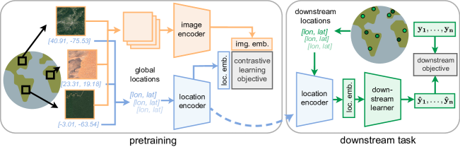
(a) Global, general-purpose pretrained location encoders.

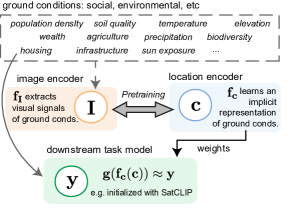
(b) Intuition behind SatCLIP.

Figure 1: Overview of the SatCLIP workflow. (a) Outlines our intuition for global, general-purpose pretrained location encoders and their deployment in downstream applications. (b) Highlights the intuition for SatCLIP: capturing ground conditions from satellite images and transferring them into a location encoder via constrastive image-location pretraining.

Much of the world’s data is geospatial. From images taken with a cellphone to the movement trajectories of taxis, different modalities live in the same geometric space: planet Earth. Geographic features, the characteristics describing any location on our planet, are commonly used in predictive modeling tasks, from using points-of-interests extracted from mapping services to predict mobility demand [43] to using satellite imagery for crop yield prediction [22]. Recent studies [24, 16, 18, 6] have also shown that explicitly providing models with intuitions for spatial and spatio-temporal dependencies (e.g., geographic priors) can help improve training and lead to more accurate predictions.

However, integrating geographic information into a deep learning model is not straightforward. Even though coordinates are often informative, introducing them as features can amplify geographic distribution shift problems and lead to poor evaluation accuracy. This is especially of concern for cross-regional generalization when data from evaluation areas (and their coordinates) are absent in the training data. As a consequence, many location-informed models are only applicable for interpolation problems where the evaluation area overlaps with the training area. While some settings warrant interpolation methods—e.g., species distribution modeling [24, 6], where data is global and somewhat representative spatially—for many applications, available labeled data is patchy and sparse, and predictive models must generalize to unseen geographic areas potentially far from the training data.

This work addresses this generalization issue by pretraining location encoders on globally and uniformly sampled satellite imagery. The location information indexing satellite images lends itself conveniently to contrastive pretraining objectives that aim to match location-image pairs. This is analogous to the text-image pretraining deployed in the popular CLIP model [30]. Furthermore, satellite imagery contains many important location characteristics (e.g. vegetation and built structures) and has proven informative in diverse downstream tasks ranging from air pollution modeling [4] to agricultural monitoring [39].

Prior investigations of pretrained location encoders hint at their potential for broad applications, but have been limited in scope for the problems we address here. Mai et al. [26] pretrain location encoders for specific applications: species distribution mapping and land cover classification. They don’t investigate the usability of their location encoders for new, out-of-domain tasks or for global generalization. In contrast, Yin et al. [45] introduce GPS2Vec with general applications in mind. However, their approach requires them to train separate location encoders for each UTM-zone. This permits them to only obtain location encoders for areas in which they have pretraining data, preventing global-scale applications.

We overcome the shortcomings of existing pretrained location encoders by designing, building, and analyzing the–to our knowledge–first general-purpose pretrained geographic location encoder with global coverage–SatCLIP. SatCLIP distills spatially varying features in global satellite data into a direct encoder of latitude and longitude, as shown in the “Pretraining” panel in Fig. 1(a). The SatCLIP pretraining objective captures the spatial variability in the appearances of images and converts them into an implicit neural representation within the location encoder. Our location encoder converts raw location coordinates into vectors that can be informative for a wide-range of environmental and socioeconomic prediction tasks, as outlined in Fig. 1(b) and demonstrated with experiments in Sec. 5. More generally, the proposed framework represents a step towards geographically-informed “foundation models” trained with large, unlabeled datasets, that are usable for a wide range of tasks, and extrapolate to unseen geographic areas. Our contributions can be summarized as follows:

• We outline the concept of pretrained geographic location encoders with global coverage. These are general-purpose models that coalesce geographic data into meaningful location embeddings, instantiated as pretrained neural networks that take global locations (latitude / longitude coordinates) as input.

• We develop the first task-generalizable, global-coverage location encoder–SatCLIP–trained on Sentinel-2 multispectral satellite imagery. We release the pretrained encoder as a PyTorch model. We also release our new pretraining dataset, S2-100K.

• We compare SatCLIP with existing pretrained location encoders and other geographic feature generation approaches on nine diverse downstream tasks, ranging from temperature prediction to population density estimation, highlighting superior performance in prediction and geographic generalization.

2 Related Work

2.1 Spatial Context from Satellite Imagery

Satellite imagery has proven to be a valuable source of input data for predictive models across a wide range of applications [32], for example, interpolating missing air pollution data [4], crop yield forecasting [39, 22], and agro-forestry carbon stock prediction [31]. In development settings, satellite-based machine learning models have helped to support humanitarian aid efforts by identifying dwellings in deprived areas [38, 44, 17], predicting poverty [12], and mapping rural populations [11].

Extracting spatial context from satellite imagery comes with several challenges. In particular, satellite imagery can be difficult and computationally expensive to obtain, store, and analyze, especially in resource-constrained settings or at a global scale. As such, providing accessible and meaningful lower-dimensional feature representations based on satellite images has been a long-standing research topic in the remote sensing literature [29]. Traditionally, geometric and object-based filtering techniques have been utilized for this task [23, 47]. More recently, Rolf et al. [32] propose using random convolutional features extracted from global-coverage satellite imagery as a conceptually simple but highly effective geographic feature extractor for inexpensive, general use in downstream prediction tasks.

These prior methods encode spatial context at different locations via embeddings of georeferenced images. In contrast, we aim to capture spatial context with models that directly take geographic coordinates as the input. We do so by training the location encoders to distill spatial variation in satellite imagery through contrastive pretraining.

2.2 Contrastive Pretraining with Geospatial Data

Unsupervised and self-supervised learning have become recent focuses for geospatial ML, as large portions of geospatial data–especially remotely sensed data like satellite imagery–are unlabeled [42]. Here, the spatiotemporal nature of geospatial data can be exploited to construct unsupervised learning objectives based on contrasting inputs from different locations or times. For example, Jean et al. [13] propose a triplet loss leveraging differences in nearby and far distant satellite image tiles for representation learning. Mañas et al. [27] exploit seasonal differences in satellite images for model pretraining and highlight performance improvements over traditional ImageNet pretraining. Scheibenreif et al. [35] and Wang et al. [41] pre-train deep learning models on multi-spectral data. To facilitate further progress in this direction, recent studies have also focused on creating and curating harmonized, multi-modal geospatial datasets [41, 20]. However, all the mentioned efforts focus exclusively on pretraining vision encoders.

Three studies have pretrained geographic location encoders that input geographic coordinates and return learned contextual representations. Yin et al. [45] propose GPS2Vec, a set of UTM-zone specific location encoders using geotagged Flickr images (YFCC100M) [37] and their corresponding semantic tags for training. Geographic generalization was out of scope for this work as embeddings are only available for UTM-zones in which training data can be found. Mai et al. [26] introduce Contrastive Spatial Pre-Training (CSP) on the iNaturalist 2018 (iNat) [10] species imagery and the Functional Map of the World (FMoW) [5] satellite image datasets. CSP is used for unsupervised pretraining and downstream prediction on the same datasets and was not conceptualized for broader, global generalization across different tasks. Just like for GPS2Vec, the pretraining datasets, iNaturalist and FMoW, are unevenly distributed over space, with high image densities in North America and Europe and few images outside of Western regions. Concurrent work of Cepeda et al. [3] proposes GeoCLIP, in which the authors pretrain image and location encoders using the MediaEval Placing Tasks 2016 (MP-16) dataset [21], also consisting of geo-tagged Flickr images. However, their work focuses on applications in geolocating images and explorations of the trained image encoder, while our objective is to train global, general-purpose location encoders.

In summary, existing work leaves two important gaps: understanding how location encoders generalize across various downstream tasks and ensuring global coverage during training.

3 Satellite Contrastive Location-Image Pretraining (SatCLIP)

With SatCLIP, we aim to train models that (1) provide general purpose embeddings and (2) are globally representative. The intuition for this framework is described next and illustrated in Fig. 1(b).

3.1 Intuition behind SatCLIP

Various factors influence the appearance of Earth’s surface, as captured in satellite images. In the top part of Fig. 1(b), we highlight that diverse environmental factors like temperature, elevation, and precipitation and socioeconomic factors like population density and agriculture contribute to the visual signature of satellite images across the globe. They are reflected in visual markers, such as the appearance of mountain ranges with their specific vegetation, the geometry and structure of agricultural fields, and the design of buildings. By training on the SatCLIP matching objective (denoted by the grey pretraining $\Leftrightarrow$ arrow and later described in Eq. 1), the image encoder $f_{\textup{I}}$ learns to associate an image with a location based on the various ground factors detectable in the images. The location encoder $f_{\textup{c}}$ learns neural implicit representations of the image features characterizing a given location. The pretrained representation models $f_{\textup{c}}$ can then be used to build spatially-aware downstream learners $g$. In our experiments, we instantiate $g$ by fine-tuning a model on top of $f_{\textup{c}}$ embeddings with annotated data in new downstream prediction tasks.

3.2 Location and Image Encoders

The inputs to a geographic location encoder are latitude/longitude coordinate pairs $\textbf{c}_{i}=[\lambda_{i},\phi_{i}]$, where $\lambda_{i}$ is the longitude, $\phi_{i}$ is the latitude, and $i$ indexes locations on the spherical surface $\mathbb{S}$. For each location $i$, we have a corresponding multi-spectral image $\mathbf{I}_{i}\in\mathbb{R}^{m\times n\times c}$ with $c$ channels. We now define two encoders, a location encoder $f_{\textup{c}}:\mathbb{S}\rightarrow\mathbb{R}^{d}$ that takes in $2$-dimensional coordinates $\textbf{c}_{i}$ and returns a $d$-dimensional latent embedding and a image encoder $f_{\textup{I}}:\mathbb{R}^{m{\times n\times c}}\rightarrow\mathbb{R}^{d}$ that takes in an image $\textbf{{I}}_{i}$ and also returns a $d$-dimensional latent embedding. Note that the image encoder can be seen as a special case of a more general context encoder that may integrate other location-specific data modalities like audio or, in the case of GPS2Vec, text.

3.3 Pretraining with the SatCLIP Objective

We train both encoders with the simple but highly effective CLIP [30] objective

$$\mathcal{L}\!=\!\frac{1}{2N}\!\left[\sum_{i=1}^{N}\!\mathcal{L}_{\textup{loc}}(\mathbf{c}_{i},\mathbf{I}_{1,\dots,N})\!+\!\sum_{i=1}^{N}\!\mathcal{L}_{\textup{img}}(\mathbf{I}_{i},\mathbf{c}_{1,\dots,N})\right]$$ (1)

that matches each coordinate $\mathbf{c}_{i}$ with the corresponding image $\mathbf{I}_{i}$ and against all images $\mathbf{I}_{1,\dots,N}$ using

$$\textstyle\mathcal{L}_{\textup{loc}}(\mathbf{c}_{i},\mathbf{I}_{1,\dots,N})=-\log\frac{\exp\left(\left\langle f_{\textup{c}}(\textbf{c}_{i}),f_{\textup{I}}(\textbf{I}_{i})\right\rangle/\tau\right)}{\sum_{j=1}^{N}\exp\left(\left\langle f_{\textup{c}}(\textbf{c}_{i}),f_{\textup{I}}(\textbf{I}_{j})\right\rangle/\tau\right)}$$ (2)

and each image with the corresponding coordinate using

$$\textstyle\mathcal{L}_{\textup{img}}(\mathbf{I}_{i},\mathbf{c}_{1,\dots,N})=-\log\frac{\exp\left(\left\langle f_{\textup{c}}(\textbf{c}_{i}),f_{\textup{I}}(\textbf{I}_{i})\right\rangle/\tau\right)}{\sum_{j=1}^{N}\exp\left(\left\langle f_{\textup{c}}(\textbf{c}_{j}),f_{\textup{I}}(\textbf{I}_{i})\right\rangle/\tau\right)}$$ (3)

over a batch $(\mathbf{c}_{i},\mathbf{I}_{i})_{i=1}^{N}$ of $N$ coordinate-image tuples. The normalized dot-product is denoted by $\langle\cdot,\cdot\rangle$, and $\tau$ is a temperature hyperparameter. This objective optimizes the weights of the location encoder $f_{\textup{c}}$ and image encoder $f_{\textup{I}}$ simultaneously to embed the feature vectors of the corresponding location $f_{\textup{c}}(\mathbf{c}_{i})\in\mathbb{R}^{d}$ and image $f_{\textup{I}}(\mathbf{I}_{i})\in\mathbb{R}^{d}$ nearby in a common $d$-dimensional feature space.

3.4 Encoder Architectures

Location encoders typically take the following form [26]:

$$f_{\textup{c}}=\textup{NN(PE}(\mathbf{c}_{i}))$$ (4)

where $\textup{PE}(\mathbf{c}_{i})$ is a nonparametric functional positional encoding and $\textup{NN}(\cdot)$ is a trainable neural network. The positional encodings usually have a resolution hyperparameter that provides control over the smoothness of spatial interpolation. The neural network weights encode an implicit neural representation of a signal at a specific coordinate [6]. In this work, we train Siren(SH) location encoders proposed by Rußwurm et al. [34]: spherical harmonics basis functions as positional encoders together with sinusoidal representation networks [36]. Rußwurm et al. [34] show that Siren(SH) location encoders are best-suited for global-scale applications without introducing artifacts at higher latitudes and poles. The degree of the spherical harmonics representation used is controlled by the number of Legendre polynomials $L$. This effectively controls the resolution of the location encoding and its capacity to learn small and large scale geospatial patterns.

As an image encoder, any vision model (e.g., a convolutional network (CNN) or vision transformer (ViT)) that is expressive enough to learn visual patterns of satellite image features is applicable. In this work, we use ResNet18, ResNet50, and ViT16 vision encoders pretrained with momentum-contrast (MoCo) [8] on Sentinel-2 satellite imagery by Wang et al. [41]. During training, we freeze the networks except for the last linear projection layer.

Table 1: Key characteristics of SatCLIP vs. the GPS2Vec and CSP location encoders and the MOSAIKS feature extractor.

	Spatial coverage	Contextual data	Location encoder	Training objective
SatCLIP (ours)	Global (continuous)	S2-100K	Spherical harmonics & Siren	Cosine similarity of embeddings (CLIP)
GPS2Vec [45]	UTM-zone specific	YFCC images	Two-level soft encoding	KL-divergence of embedding distributions
	(mostly Europe and North America)	and semantic tags
CSP [26]	Global (continuous)	FMoW, iNaturalist	Sinusoidal transform & FcNet	Cosine similarity of embeddings (CLIP)
				+ negative location sampling + SimCSE
MOSAIKS [32]	Global (0.01∘ grid)	Planet Basemaps	N/A (direct feature extractor)	None

3.5 SatCLIP Pretraining Details

We pretrain SatCLIP using the S2-100K dataset (described in Sec. 4.1). We use $90\%$ of the data points, selected uniformly at random, for pretraining and reserve the remaining $10\%$ as a validation set to monitor overfitting. During pretraining, we found that batch sizes of $8k$ help the model to learn more fine-grained representations, while too large batch sizes can prevent learning. This supports the findings of recent work on CLIP models [46]. We train models for $500$ epochs on an A100 GPU. More pretraining details can be found in Appendix C.

3.6 SatCLIP Fine-tuning Details

To test the general applicability of the location embeddings, we run experiments on a wide range of out-of-domain geospatial predictive modeling tasks (i.e., tasks not involving multi-spectral satellite imagery). In all datasets, the inputs are raw latitude/longitude coordinates, which we transform into location embeddings. For the iNaturalist 2018 classification, we have additional input image features extracted from an InceptionV3 model released by [24] which we concatenate with location embeddings during downstream training.

We train multi-layer perceptron (MLP) models with location embeddings as input for all tasks using the Adam [15] optimizer. Regression models use a mean squared error (MSE) loss, and classification models use cross-entropy loss. Hyperparameters like learning rate, number of layers, or hidden dimensions are tuned using a random search on an independent validation set. All results are reported for an unseen test set. More details on the training setting can be found in Appendix E.

3.7 Comparison Methods

We compare trained SatCLIP location encoders to GPS2Vec [45] and CSP [26] pretrained location embeddings. We refer to each comparison model by first stating the pretraining algorithm and then the pretraining dataset. For instance, CSP-FMoW represents CSP pretraining on the Functional Map of the World (FMoW) [5] dataset. CSP [26] use a sine-cosine-based positional encoding (grid [25]) together with a 4-layer multi-layer perception (MLP) with skip connections termed FcNet, proposed initially by [24] as location encoder, and InceptionV3 and ResNet50 models for iNat 2018 and FMoW data, respectively. GPS2Vec [45] encodes locations by combining an exponential functional transform of each coordinate and its respective UTM-zone centroid with a simple three-layer ReLu network, and extracts text and image context features via vocabulary-based and CNN approaches.

We also compare to a further, non-pretraining-based global feature extractor: MOSAIKS [32]. For a given latitude/longitude pair, the MOSAIKS featurization returns random convolutional features extracted from the nearest gridded satellite image. We access pre-computed MOSAIKS features from siml.berkeley.edu [2], which provides image features derived from Planet Basemaps from 2019, Quarter 3, at a gridded resolution of $0.01^{\circ}$.

A comparison between the key characteristics of SatCLIP and all comparison methods can be found in Tab. 1. Further details on these methods and their pretraining datasets are given in Appendix B.

4 Datasets

4.1 S2-100K: Near-uniformly Distributed Sentinel-2 Images

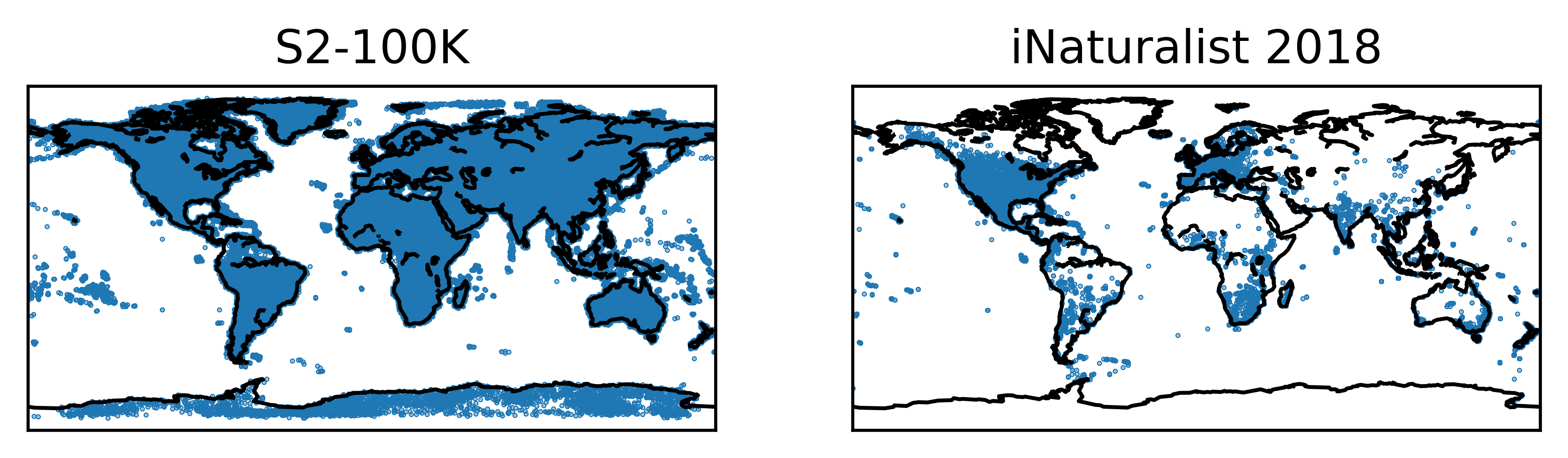
Figure 2: Spatial distribution of the S2-100K dataset used for training SatCLIP compared with iNaturalist 2018 [10], which is used to pretrain one of the CSP models. iNaturalist heavily overrepresents North America and Europe.

To construct our pretraining dataset, S2-100K, we sample $100,000$ tiles of multi-spectral ($12$-channel) Sentinel-2 satellite imagery and their associated centroid locations uniformly at random from locations where Sentinel-2 imagery is available. More details of the S2-100K dataset are provided in Appendix A. The dataset is availabe for download at https://github.com/microsoft/satclip/. We design the S2-100K dataset with the goals of multi-task applicability and geographic generalization performance in mind. Our dataset (1) represents general location features by using multi-spectral satellite imagery (as illustrated in Fig. 1) and (2) is nearly uniformly distributed across global land mass (Fig. 2, left).

In contrast, the pretraining datasets used in comparison methods (Sec. 3.7) often significantly underrepresent certain–especially non-Western–geographic areas. Fig. 2 illustrates the spatial coverage of S2-100K compared to the highly clustered distribution of iNaturalist, which is used as a pretraining dataset for CSP [26]. Similar biases are exhibited by the Yahoo-Flickr Creative Commons 100 Million (YFCC100M) dataset [37] of image-tag-location triplets (used in GPS2Vec), and the Functional Map of the World (FMoW) [5] dataset, which samples satellite imagery mostly near human built infrastructure (also used in CSP). The pretraining datasets used by comparison methods (Sec. 3.7) are described in detail in Appendix B.

4.2 Downstream Tasks

The nine downstream datasets used in this work span socioeconomic and environmental applications. The variety of datasets allows us to examine whether features captured by a SatCLIP-pretrained location encoder are useful across a broad range of tasks. We predict variables including Air Temperature [9] and Elevation [32] from coordinates as environmental regression objectives. To capture socioeconomic factors, we regress Median Income [14], California Housing prices [28], and logged Population Density [32]. We additionally classify iNaturalist species [10], Biomes, and Eco-regions [7] and compile a new country code classification task Countries. In our experiments, we fine-tune encoders to each dataset and compare the performance of our pretrained SatCLIP embeddings with other pretrained location encoders (CSP, GPS2Vec) and unsupervised image features (MOSAIKS) found in the literature. More details on all downstream tasks can be found in Sec. E.2.

5 Experiments

Table 2: Downstream task performance using SatCLIP ($L=40$) vs. baseline location embeddings. We report average test set MSE and accuracy $\pm 1$ standard deviation across $10$ independently initialized MLP training runs.

	SatCLIP-RN50	SatCLIP-ViT16	CSP	CSP	GPS2Vec	GPS2Vec	MOSAIKS
Task $\downarrow$ Data $\rightarrow$	(S2-100K)	(S2-100K)	(FMoW)	(iNat)	(tag)	(visual)	(Planet)
Regression	MSE $\downarrow$
Air temperature	$\mathbf{0.27\pm 0.03}$	$\mathbf{0.25\pm 0.02}$	$2.81\pm 1.11$	$4.71\pm 1.78$	$2.37\pm 0.00$	$2.92\pm 0.01$	$4.61\pm 6.05$
Median income	$\mathbf{0.71\pm 0.16}$	$\mathbf{0.67\pm 0.01}$	$1.39\pm 0.07$	$1.35\pm 0.03$	$1.06\pm 0.00$	$1.31\pm 0.00$	$1.31\pm 0.07$
Cali. housing	$2.42\pm 0.12$	$2.62\pm 0.28$	$5.67\pm 0.00$	$5.68\pm 0.01$	$\mathbf{1.64\pm 0.15}$	$2.20\pm 0.14$	$4.30\pm 0.11$
Elevation	$\mathbf{0.15\pm 0.00}$	$\mathbf{0.15\pm 0.01}$	$0.80\pm 0.05$	$1.11\pm 0.06$	$1.11\pm 0.01$	$1.17\pm 0.00$	$0.98\pm 0.01$
Population	$\mathbf{0.48\pm 0.01}$	$\mathbf{0.50\pm 0.02}$	$1.69\pm 0.16$	$1.72\pm 0.28$	$1.99\pm 0.00$	$2.28\pm 0.00$	$1.45\pm 0.05$
Classification	% Accuracy $\uparrow$
Countries	$\mathbf{96.00\pm 0.14}$	$95.77\pm 0.14$	$77.78\pm 1.66$	$82.11\pm 1.72$	$70.35\pm 0.06$	$67.80\pm 0.03$	$76.16\pm 0.50$
iNaturalist	$\mathbf{66.03\pm 0.54}$	$\mathbf{65.98\pm 0.61}$	$56.73\pm 0.83$	$60.47\pm 0.56$	$58.78\pm 0.48$	$53.27\pm 0.78$	$56.73\pm 0.80$
Biome	$\mathbf{94.41\pm 0.14}$	$\mathbf{94.27\pm 0.15}$	$75.81\pm 1.53$	$73.18\pm 5.58$	$69.69\pm 0.06$	$68.29\pm 0.11$	$79.61\pm 0.42$
Ecoregions	$\mathbf{91.67\pm 0.15}$	$\mathbf{91.61\pm 0.22}$	$76.87\pm 1.27$	$78.43\pm 1.71$	$68.46\pm 0.06$	$67.26\pm 0.02$	$70.48\pm 0.21$

In our experiments, we focus on three research questions: How generalizable are SatCLIP embeddings from S2-100k data across a diverse range of geospatial modeling tasks (RQ 1) and across geographic areas (RQ 2) compared to existing pretrained location encoders? Lastly, following the intuition of Fig. 1, we ask: Do SatCLIP embeddings capture spatial trends in diverse underlying social and environmental ground conditions? (RQ 3). Code for SatCLIP pretraining and downstream experiments is available at https://github.com/microsoft/satclip.

5.1 Downstream Task Performance (RQ 1)

We use the SatCLIP-pretrained location encoders as input to a model which we fine-tune for each downstream task separately, as detailed in Sec. 3.6. In Tab. 2, we show performance across the different downstream tasks, in comparison to existing methods (detailed in Sec. 3.7). SatCLIP embeddings achieve the best prediction scores by a large margin on eight of the nine datasets. The exception is the California Housing dataset, which is limited to California and perhaps more adequately represented by YFCC-100M, the pretraining dataset underlying the GPS2Vec model.

Generally, our evaluation setup including multiple, diverse tasks is out-of-scope for both CSP [25] and GPS2Vec [45], which are trained for in-domain deployment. Of the existing methods, only MOSAIKS [32] investigate the generalization of their method across different tasks.

Fig. 3 highlights the performance of SatCLIP and existing location encoders when evaluated separately for each continent. SatCLIP performs well on all continents, achieving the best performance on each continent with relatively small variation in performance across continents. Prior location encoders (CSP and GPS2Vec) trained on spatially biased training data tend to perform best in Europe and North America, with performance drops in the underrepresented continents of Africa, Asia, and South America.

5.2 Zero/Few-Shot Geographic Adaptation (RQ 2)

Table 3: Geographic adaptation capabilities of SatCLIP ($L=40$) vs. baseline location embeddings to new geographic areas with no ($*$) or very few ($\dagger$) samples from the held-out test continent. We report average test set MSE and accuracy in % $\pm 1$ standard deviation across $10$ independently initialized MLP fine-tuning runs.

	SatCLIP-RN50	SatCLIP-ViT16	CSP	CSP	GPS2Vec	GPS2Vec	MOSAIKS
Test Continent	(S2-100K)	(S2-100K)	(FMoW)	(iNat)	(tag)	(visual)	(Planet)
Asia
Air Temp.∗ MSE $\downarrow$	$1.50\pm 0.10$	$\mathbf{1.26\pm 0.15}$	$3.06\pm 1.24$	$5.07\pm 4.45$	$16.70\pm 16.50$	$4.15\pm 0.58$	$10.56\pm 11.82$
Elevation∗	$3.28\pm 0.09$	$\mathbf{2.06\pm 0.28}$	$4.73\pm 0.29$	$4.98\pm 0.13$	$5.09\pm 0.06$	$4.92\pm 0.02$	$4.22\pm 0.23$
Pop. Density∗	$2.82\pm 0.22$	$\mathbf{1.94\pm 0.15}$	$4.53\pm 0.38$	$7.10\pm 1.14$	$4.84\pm 0.13$	$5.54\pm 0.03$	$3.35\pm 0.43$
Countries† % Acc. $\uparrow$	$14.29\pm 1.62$	$\mathbf{19.17\pm 2.82}$	$1.22\pm 0.05$	$1.28\pm 0.01$	$1.12\pm 0.00$	$0.92\pm 0.02$	$1.56\pm 0.47$
iNaturalist∗	$17.67\pm 0.32$	$20.91\pm 0.77$	$19.85\pm 0.55$	$\mathbf{21.49\pm 0.85}$	$17.52\pm 0.38$	$18.11\pm 0.34$	$16.14\pm 0.42$
Biome∗	$30.26\pm 3.00$	$16.44\pm 1.21$	$1.98\pm 0.62$	$3.00\pm 2.60$	$1.76\pm 0.04$	$2.79\pm 0.19$	$\mathbf{37.81\pm 4.47}$
Ecoregions†	$8.46\pm 0.79$	$\mathbf{10.86\pm 1.19}$	$1.55\pm 0.17$	$1.41\pm 0.14$	$1.49\pm 0.03$	$1.48\pm 0.00$	$1.36\pm 0.10$
Africa
Air Temp.∗ MSE $\downarrow$	$\mathbf{2.17\pm 0.33}$	$\mathbf{1.79\pm 0.50}$	$3.35\pm 2.30$	$2.65\pm 4.19$	$6.44\pm 0.03$	$5.99\pm 0.19$	$13.32\pm 13.27$
Elevation∗	$0.81\pm 0.06$	$\mathbf{0.57\pm 0.04}$	$0.66\pm 0.04$	$1.05\pm 0.26$	$\mathbf{0.54\pm 0.03}$	$\mathbf{0.55\pm 0.01}$	$0.85\pm 0.20$
Pop. Density∗	$2.99\pm 0.23$	$\mathbf{1.96\pm 0.22}$	$3.64\pm 0.49$	$3.10\pm 0.39$	$3.19\pm 0.06$	$3.25\pm 0.01$	$\mathbf{2.03\pm 0.12}$
Countries† % Acc. $\uparrow$	$\mathbf{8.95\pm 1.04}$	$\mathbf{10.22\pm 1.62}$	$0.47\pm 0.01$	$0.45\pm 0.04$	$0.47\pm 0.01$	$0.45\pm 0.00$	$0.48\pm 0.00$
iNaturalist∗	$5.22\pm 0.26$	${6.23\pm 0.47}$	${6.63\pm 0.57}$	$\mathbf{8.65\pm 0.52}$	$7.47\pm 0.53$	$6.85\pm 0.39$	$5.18\pm 0.38$
Biome∗	$33.77\pm 2.69$	$12.34\pm 1.75$	$0.94\pm 0.00$	$1.09\pm 0.48$	$1.29\pm 0.04$	$1.17\pm 0.21$	$\mathbf{49.86\pm 1.57}$
Ecoregions†	$\mathbf{13.54\pm 2.06}$	$\mathbf{12.91\pm 1.63}$	$0.90\pm 0.00$	$0.94\pm 0.04$	$0.88\pm 0.01$	$0.90\pm 0.00$	$0.92\pm 0.12$
# wins of 14 total tasks	3	10	0	2	1	1	3

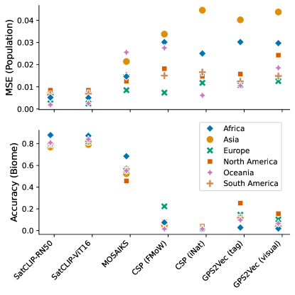
Figure 3: Performance metrics aggregated by continent highlight how location embeddings perform in different geographic areas for population density estimation and biome classification. For the SatCLIP models, we use L=40.

Next, we test whether our embeddings can help overcome the challenges of geographic domain shift. Geographic domain shift describes distributional changes in data across geographic areas and is an important challenge in environmental problems like species distribution modeling [1], land cover classification [33], crop type mapping [19], and crop yield prediction [39].

Here, the implicit neural representation of environmental factors within the SatCLIP location encoder may provide additional location-specific information about the ecological niches of species and support generalization with no or few data points in the target area. To test for this setting, we deploy a spatial train/test split strategy: We hold out specific continents, either Africa or Asia, as test sets and use the remaining data for model training and validation. Since the Countries and Ecoregions class labels are unique to each continent, for those two tasks, we add a small portion of the test continent points to the training set ($1\%$ selected uniformly at random) to create a de-facto few-shot geographic adaptation setting. For the remaining tasks, we test zero-shot adaptation by not providing any training points from the held-out test continent. In iNaturalist 2018, for example, this means that the model will not be able to recognize any species that are endemic to the test continent (i.e., that do not live in any other continent). However, we can assess whether the model recognizes known species that appear in the unseen continent.

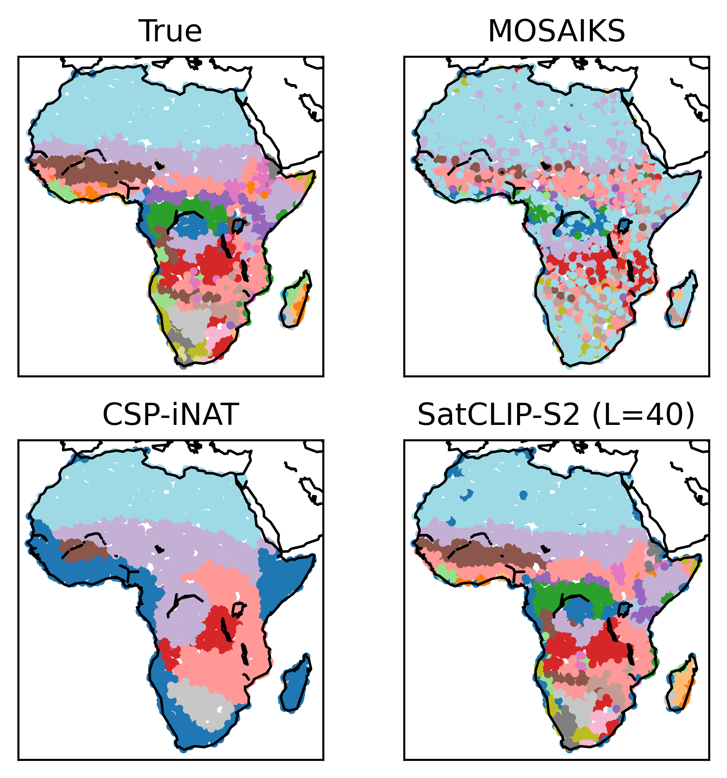
Figure 4: Geographic adaptation. Predictions of ecoregions on the unseen test continent Africa. The SatCLIP model shown uses a ResNet50 vision encoder.

Tab. 3 shows the regression MSE and classification accuracy over the held-out continents, as detailed above. Models trained with SatCLIP embeddings can adapt to the unseen geographic areas with zero (tasks marked by ^∗) or very few (tasks marked by ^†) fine-tuning samples. SatCLIP models are often (but not always) better than the comparison approaches across both held-out continents. We highlight this with results on the Ecoregions dataset in Fig. 4. In particular, for the iNaturalist downstream task, the SatCLIP location encoder only falls behind the iNaturalist-pretrained CSP of Mai et al. [26], which has a natural advantage in this case. Overall, these results indicate that Sentinel-2 data contains features that can, to some degree, generalize across the planet and across application domains–and, that this information can be encoded directly into a context-pretrained location encoder.

5.3 Analysis of Location Embeddings (RQ 3)

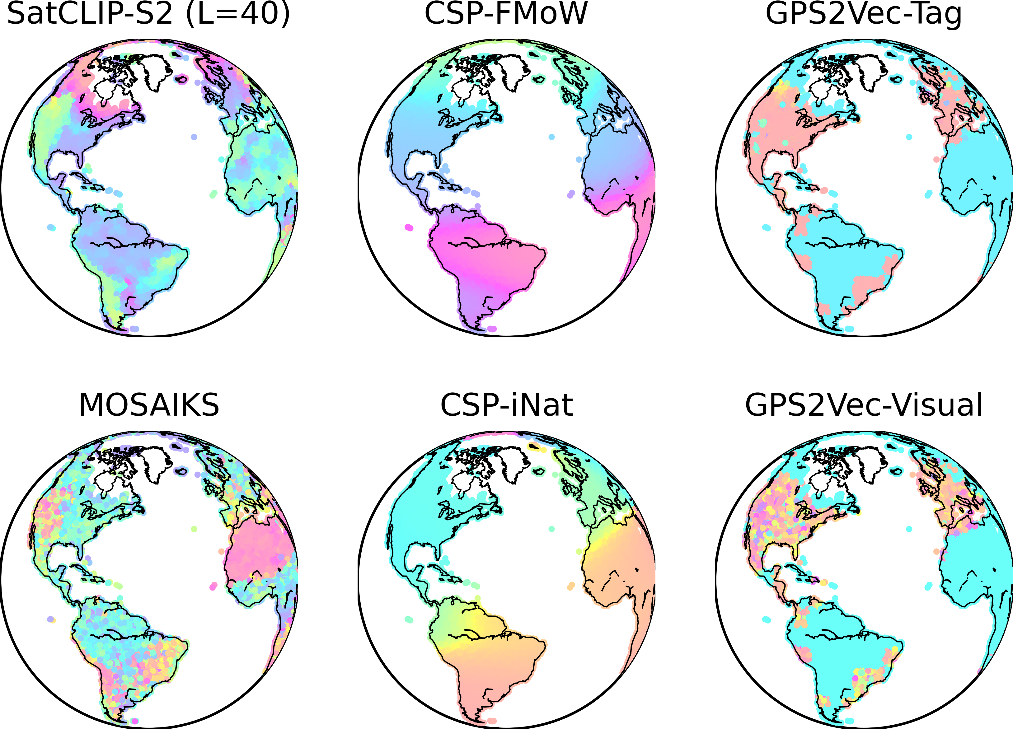
(a) Latent space visualization: Top-$3$ principal components as RGB.

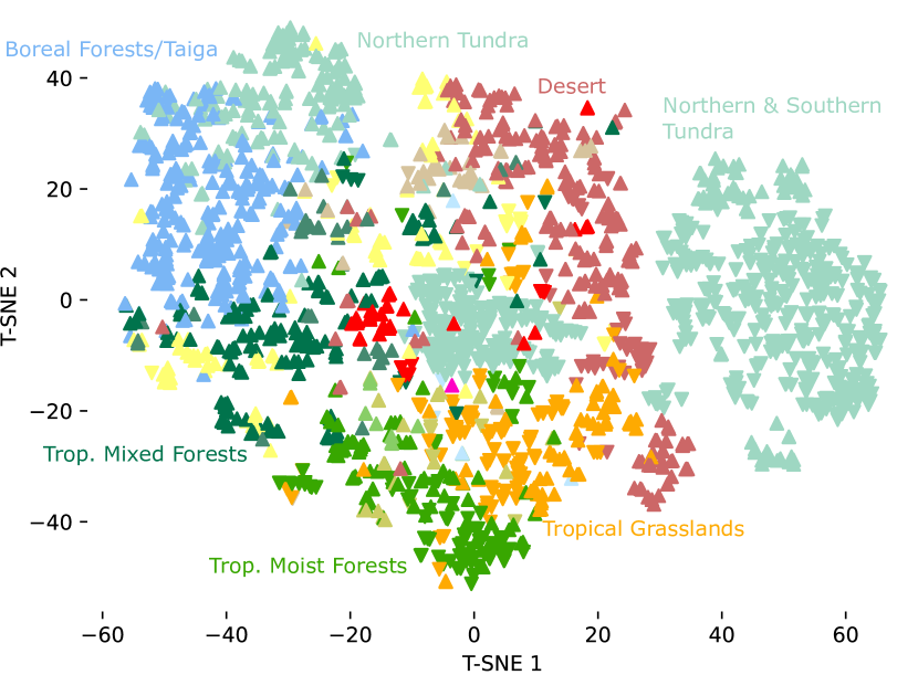
(b) Analysis of environmental factors learned by the trained SatCLIP location encoder by a T-SNE [40] dimensionality reduction at globally distributed points colored by biome type. Overall, biomes are clearly separated in this T-SNE embedding space. Note that some points of the northern $\triangle$ and southern $\triangledown$ hemispheres are mapped nearby, which indicates that this clustering is due to the trained SatCLIP weights and not the pure coordinates, as we investigate further in the appendix Fig. 7.

Figure 5: Analysis of SatCLIP-trained coordinate embeddings.

We now investigate qualitatively to what degree the SatCLIP embeddings have learned an implicit representation of different ground conditions in the location encoder weights. We first visualize a low-dimensional projection of the latent representations learned by our location encoders. Fig. 5(a) shows an RGB representation of the first three principal components of embeddings at locations around the planet. The figure highlights how embeddings learned by SatCLIP provide fine-grained representations of different locations (expressed by different colors), capturing global patterns like climate zones. In comparison, other methods are globally very coarse (CSP) or exhibit most of their spatial variation only in isolated regions across the globe (GPS2Vec).

Next, we analyze to what degree environmental ground conditions have been learned in the SatCLIP location encoder (trained with the RN-50 image encoder). We embed random globally distributed land coordinates with the SatCLIP location encoder ($L=40$) into a 256-dimensional feature space and project it into a 2-dimensional visualization in Fig. 5(b) using t-distributed stochastic neighborhood embedding (T-SNE) [40] (perplexity=$30.0$). The embedded points are colored by the biomes corresponding to their geographic coordinate. We mark points on the northern and southern hemispheres by $\triangle$ and $\triangledown$, respectively.

From Fig. 5(b), we can see that different biomes are clustered in the embedding space learned by the SatCLIP-trained location encoder. Tropical (wet) biomes are located in the lower part (negative T-SNE 2), while increasingly drier biomes (Tropical Grasslands $\rightarrow$ Desert & Tundra) are generally located towards the upper right of this embedding projection. This embedding visualization incorporates the joint effect of learned environmental characteristics and coordinate locations, as shown in the split of the Tundra biomes in three clusters: one for the northern hemisphere ($\triangle$), one for the southern hemisphere ($\triangledown$), and a third that incorporates samples from both northern and southern hemispheres that we believe is connected to the unique environmental properties of the dry and cold Taiga climate. We disentangle this double effect of pure coordinate embedding and trained weights in Appendix D. There, we show that a pure coordinate embedding cannot separate the biomes as clearly and rather produces one long manifold following geographic topology. In summary, this clear biome-wise clustering explains the above 90% accuracy of SatCLIP-RN50 on the Biome classification task (Tab. 2) and qualitatively supports our intuition behind SatCLIP as a method to learn representations of environmental factors from satellite images (Fig. 1).

6 Discussion and Conclusion

In this work, we train a location encoder that learns an implicit neural representation of remote sensing data by matching satellite images and their respective coordinates using the CLIP objective. Our experiments show that such a representation can provide useful information for a wide range of downstream tasks and help models to generalize to unseen geographic areas with no or little training data, which is a key challenge in geospatial machine learning.

The embeddings learned through our SatCLIP models are highly descriptive of socioeconomic and environmental features at different locations. Overall, the simple but effective SatCLIP framework lays the foundation for a new class of models: global-coverage, general-purpose location encoders that coalesce large, geo-tagged data into a succinct representation of any location.

Two key factors contribute to the exceptional performance improvements observed in Secs. 5.1 and 5.2. First, we pretrain SatCLIP on a uniformly distributed S2-100K dataset that provides the necessary support for globally distributed downstream tasks. Second, we use the recently proposed Siren(SH) location encoder [34], which has proven to be well suited for global and continental-scale representation of data on the spherical Earth. One limitation of our work is its focus on a single data modality for pretraining: While matching coordinates with free satellite imagery makes our model training easily applicable, additional expressiveness and downstream accuracy can likely be gained by including additional data sources.

The CLIP objective is not limited to image-coordinate matching. Joint location-specific information could be similarly extracted using generic context vectors, such as text from geolocated social media posts, or point-of-interest data available in geodatabases. This can be integrated by simultaneously pretraining on different modalities to distill socioeconomic and environmental factors present in other modalities beyond satellite images. In future work, we aim to build location encoders that incorporate multiple data modalities and include temporal as well as spatial information.

Supplementary Material

Appendix A S2-100K Dataset Overview

We sample the S2-100k dataset from all Sentinel 2 Level-2A scenes that meet the following criteria:

1. Are captured between January 1st, 2021 and May 17th, 2023

2. Are estimated to have less than 20% cloud cover (as reported by the European Space Agency preprocessing)

3. Are at least partially over a land mass (measured with country level boundaries from gadm.org)

Using the Microsoft Planetary Computer, we find $2,359,972$ S2-L2A scenes that meet these criteria. We sample a random scene, sample a random $256\times 256$ pixel patch from that scene, then keep the patch if less than 10% of the pixels include nodata values, else we reject the patch. We repeat this process until we have $100,000$ patches. Each patch contains all available bands – B01, B02, B03, B04, B06, B06, B07, B08, B08A, B09, B11, and B12 – resampled to a 10m/px spatial resolution in the native UTM coordinate system and saved as a single Cloud Optimized GeoTIFF. Finally, we record the latitude and longitude (using the EPSG:4326 coordinate system) of the center point of the patch. The dataset can be downloaded at https://github.com/microsoft/satclip/. The final dataset is $83.79$ Gigabytes on disk.

Appendix B Further Details on Other Pretrained Location Encoders

B.1 Training Data

Here, we describe the datasets used for pretraining in previous geographic location encoders, CSP and GPS2Vec, in detail:

iNat 2018 [10]: This dataset contains crowdsourced, natural images of over $8,000$ plant and animal species from around the globe. The iNat 2018 training set contains over $400,000$ image-location pairs. While species distributions can be indicative of e.g., climate zones [24], they are less descriptive of socio-economic processes, as we show in our experiments. Furthermore, most iNat image locations lie in North America and Europe, with only few observations in other continents, as we show in Fig. 2. We obtain location encoders pretrained on iNat from CSP [26].

FMoW [5]: This dataset contains satellite images annotated with bounding boxes representing $63$ categories describing functional or land-use characteristics (e.g., “airport” or “gas station”). The dataset contains over $363,000$ image-location pairs. FMoW is aimed to support detection of functional objects from satellite imagery and, as such, is skewed towards human-built infrastructure and includes fewer natural scenes. It is also again heavily favoring Western countries in its geographic distribution. We obtain location encoders pretrained on FMoW from CSP [26].

YFCC100M [37]: This dataset contains natural images and associated semantic tags collected from the social media platform Flickr. YFCC100M includes approximately $48$ million image-tag-location triplets. Images (and tags) represent diverse scenes, from street views to birthday parties. While they are more indicative of social dimensions and physical infrastructure, YFCC100M imagery is less representative of natural processes. Just like iNat and FMoW, the dataset again mostly contains locations in Western countries. We obtain models separately trained on images and semantic tags from GPS2Vec [45].

B.2 CSP

Location and image encoders: The authors use a location encoder combining sinusoidal transforms introduced by [25] with a fully-connected neural network. The image encoder is dataset-dependent. For the iNat dataset, the authors use a pretrained IncpetionV3 network. For the FMoW dataset, they use a pretrained ResNet50 network. In both cases, neural network weights in all layers except the last linear projection layer are frozen.

Learning objective: Here, the authors combine (1) the standard CLIP loss, which leverages in-batch negative sampling and which is also used by us, with two other contrastive objectives: (2) Random negative location sampling (i.e. predicting the real location from a set of randomly generated locations) and (3) SimCSE sampling (i.e. matching location embeddings obtained using different dropout masks). The two extra objectives help the model to balance the location and context encoders. We find that the two additional objectives are not needed for training SatCLIP.

B.3 GPS2Vec

Location and context encoders: The authors train location encoders specific to the UTM zones containing training data. They first encode coordinates as an exponential function of the Euclidean distance between a latitude/longitude coordinate and its respective UTM zone centroid coordinate. This is followed by a simple ReLu network with three hidden layers. GPS2Vec does not learn a context encoder but directly extracts text features using a vocabulary-based approach and image features using convolutional neural networks (CNN).

Learning objective: The authors design an objective which aims to use contextual features (images and semantic tags) as labels to train their location encoder by estimating the normalized frequency of features in the vicinity of a given location. Practically, this is achieved by minimizing the KL-divergence of context and location embedding distributions.

Appendix C SatCLIP training

C.1 Training Details

Batch size: After experimenting with different batch sizes, we opt for models trained at batch sizes of $8k$. While traditional CLIP image-text pretraining behaves optimally at a batch size of $32k$ [46], we observe that this prevents effective training.

Image encoder: We train SatCLIP models with ViT16, ResNet18 and ResNet50 image encoders, all pretrained on Sentinel-2 imagery and published by [42]. We keep the image encoders frozen during training, and only train a last projection layer that maps the image embeddings into the desired output space. We find this to be ideal for training at a size of $256$–this is equivalent to the embedding size used by CSP [26].

Location encoder: Our location encoder follows an approach recently proposed by [34]. It first puts raw latitude/longitude coordinates through a functional transform based on orthogonal spherical harmonics. The number of spherical harmonics used corresponds to the resolution at which the model is trained. In practice this is controlled by a parameter defining the number of Legendre polynomials $L$ used for spherical harmonics computation. We train a lower-resolution ($L=10$) and a higher-resolution ($L=40$) version of SatCLIP. The functional transform is followed by a sinusoidal representation network (Siren) consisting of two hidden layers and $512$ hidden dimensions. These hyperparameters are obtained after rigurously testing different settings.

Augmentations: We deploy several data augmentations within our training procedure. Image augmentations include random crops, random horizontal flipping, random vertical flipping and Gaussian blurs. Point coordinates are augmented using a coordinate jitter which randomly shifts image coordinates by up to about 1km.

Optimization: All SatCLIP models are trained with the Adam optimizer, a learning rate of $0.0001$ and a relatively high weight-decay values of $0.01$ to help prevent overfitting. All final SatCLIP models are trained for $500$ epochs. On our single A100 GPU, training takes around $2$ days. Throughout training, we reserve $10\%$ of the data for validation. We monitor validation loss and select SatCLIP models according to the minimum validation loss.

C.2 Scale Sensitivity

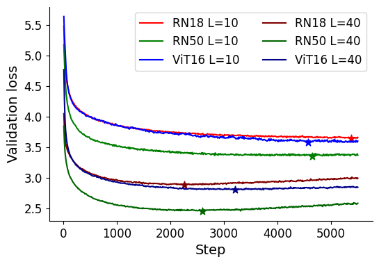
Figure 6: Validation set loss of SatCLIP models trained with different vision encoder backbones (ResNet18, ResNet50 and ViT16) with $L=10$ and $L=40$. Stars indicate the minimum validation loss, which we use for model selection.

We want to briefly comment on the sensitivity of SatCLIP training to the number of legendre polynomials $L$ used in the model’s spherical harmonics location encoder. This hyperparameter effectively controls the spatial resolution of the obtained embeddings. Smaller values of $L$ are computationally more efficient and ideal for representing large-scale patterns, while larger values of $L$ are better for capturing small-scale patterns. More details on this can be found in Rußwurm et al. [34]. During SatCLIP training, we observe some interesting differences between smaller ($L=10$) and higher ($L=40$) resolution models. We find that higher-resolution models are more likely to exhibit overfitting, as Fig. 6 highlights. On downstream tasks, higher resolution models perform better at smaller scale, regional tasks as e.g. the Cali. Housing dataset, as Tab. 6 highlights. Lastly, $L=40$ models appear better for spatial interpolation (RQ1), while $L=10$ models seem better suited for geographic generalization (RQ2).

Appendix D Latent Space Exploration

D.1 SatCLIP Embeddings in Different Biomes

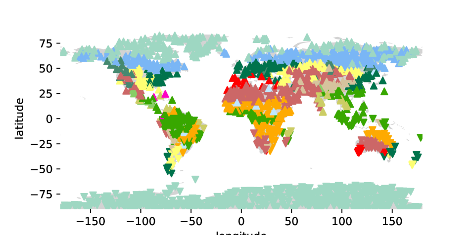
(a) Map (lon/lat) representation of all biomes

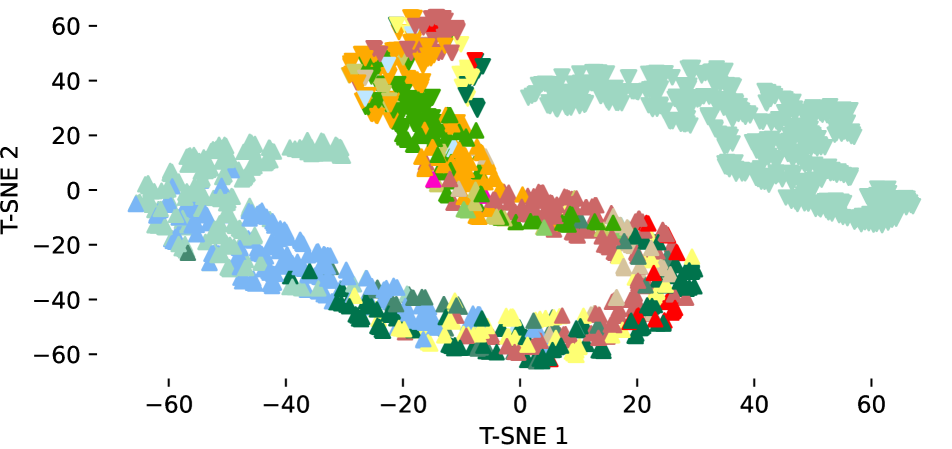
(b) Spherical harm. (SH) embedding (no weights).

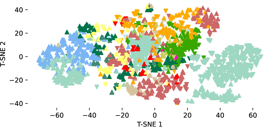
(c) SatCLIP (SH & trained SirenNet)

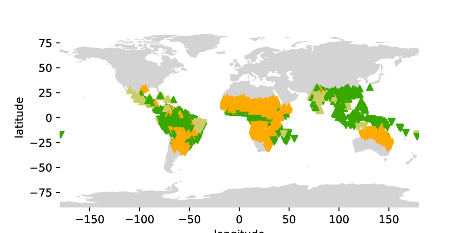
(d) Difficult-to-separate tropical biomes

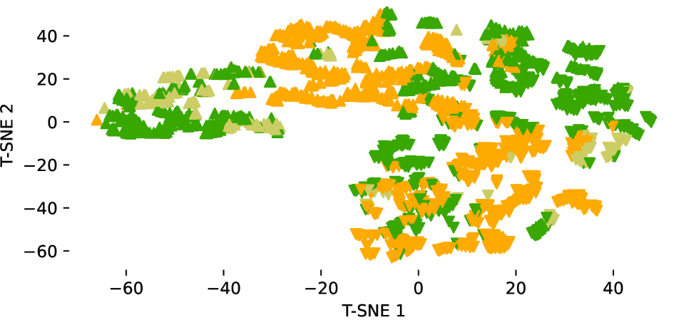
(e) Spherical harm. (SH) embedding (no weights).

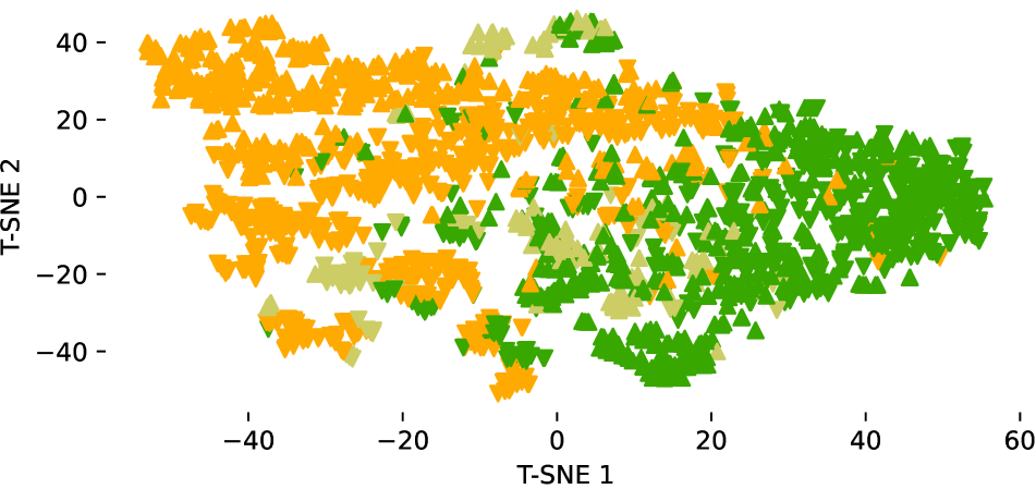
(f) SatCLIP (SH & trained SirenNet)

Figure 7: Supplementary experiment to Fig. 5(b): we disentangle the influence of spherical harmonic (SH) coordinate embedding without trainable weights in Figs b) & e) with the trained SatCLIP location encoder in Figs c) & f). Comparing the T-SNE embedding projections in these two columns reveals the additional effect of having trained SatCLIP weights int he location encoder. We perform this analysis in an easier setting with all biomes (top row) and with only tropical geographically intertwined biomes (bottom row). In the top row, also the pure spherical harmonic basis functions produce a T-SNE manifold along which biomes are located b). In the more difficult bottom row, no coherent manifolds form in e) along biome types. These appear only in combination with the SatCLIP-trained weights in f)

This supplementary experiment disentangles the influence of raw coordinates and learned SatCLIP embeddings in the T-SNE embedding experiment of Fig. 5(b) in the main paper that indicated that the SatCLIP weights encode environmental factors like dryness or temperature in biomes. Critically speaking, also the direct embedding of coordinates without any weights could generate T-SNE clusters that look similar to Fig. 5(b). In Fig. 7, we investigate if this is the case by showing the embeddings of coordinates with Spherical Harmonics (SH) (no trainable weights) alone (Figs. 7(b) and 7(e)) and compare it with the trained SatCLIP location encoder, which combines Spherical Harmonics basis functions with Sinusoidal Representation Networks (SirenNets) [36] (Figs. 7(c) and 7(f)).

In the top row Figs. 7(c), 7(b) and 7(a) we show all biomes and can see that the T-SNE points embedded in spherical harmonic basis functions of pure coordinates (without trainable weights) (Fig. 7(b)) creates a clear manifold along which the different biomes cluster. However, notice that points from the northern hemisphere ($\triangle$) are clearly separated from the southern hemisphere ($\triangledown$). Also, the arctic and antarctic tundra biomes are separated by two clusters. This is the T-SNE embedding produced from pure coordinate embeddings, that serves as the baseline to the SatCLIP embeddings that are produced by representing point coordinates as spherical harmonic basis functions and transforming these basis functions with the SatCLIP-trained SirenNet neural network. The result is shown in Fig. 7(c), which corresponds to Fig. 5(b) in the main paper, where the embedding clusters along dryness and temperature dimensions rather than pure geographic location. Hence, by comparing Fig. 7(b) (no weights) with Fig. 7(c), we can see the effect of trainable SatCLIP weights on the T-SNE representation of the points.

To make sure that this analysis holds, we repeat the embedding in a more challenging setting: we show embeddings of points from only tropical biomes for (Sub-)Tropical Moist Broadleaf Forests, (Sub-)Tropical Dry Broadleaf Forests, and (Sub-)Tropical Grasslands, Savannas & Shrublands in Figs. 7(f), 7(e) and 7(d) (second row). Points from these biomes are not separable using only non-parametric embeddings (Fig. 7(e)), since these biomes are all tropical and geographically intertwined. Here only the geographic coordinate is not sufficiently expressive to form T-SNE manifolds along biome lines. However, with the pretrained SatCLIP location encoder (Fig. 7(f)), we can clearly identify a dry to wet trend along T-SNE dimension 1 (left to right) where points from grassland/savanna transitions first into dry broadleaf forest and then moist broadleaf forest.

In summary, these supplementary analyses reinforce the conclusions of the main paper experiment around Fig. 5(b), which experimentally supports the concept that the SatCLIP embeddings represent an implicit neural representation of environmental and societal ground conditions that are visible in the Sentinel-2 images that the SatCLIP model is trained on.

D.2 Latent Space Visualization at Different Scales

Lastly, we provide a visualization of the embeddings learned by SatCLIP models at different scales (different $L$ values) in Fig. 8. It is clearly visible how SatCLIP $L=40$ resolves positional embeddings much more fine-grained. Lastly, in Fig. 9 we show the explained variance ratio by element in a respective embedding vector, extracted via PCA, including SatCLIPs with different $L$ values and comparison methods.

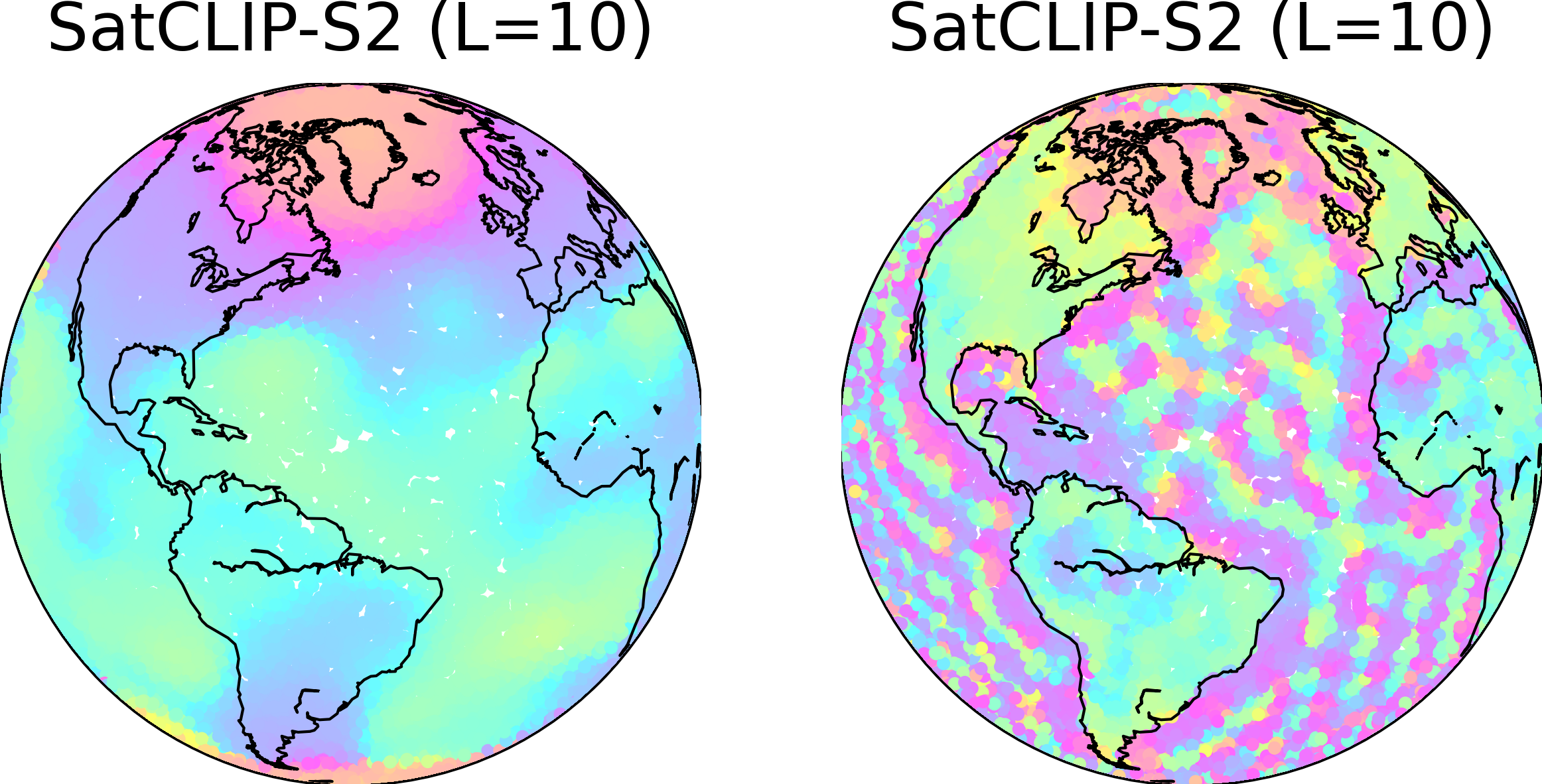
Figure 8: Visualization of the top-$3$ principal components, plotted as RGB channels, of SatCLIP models trained with different $L$ hyperparameters.

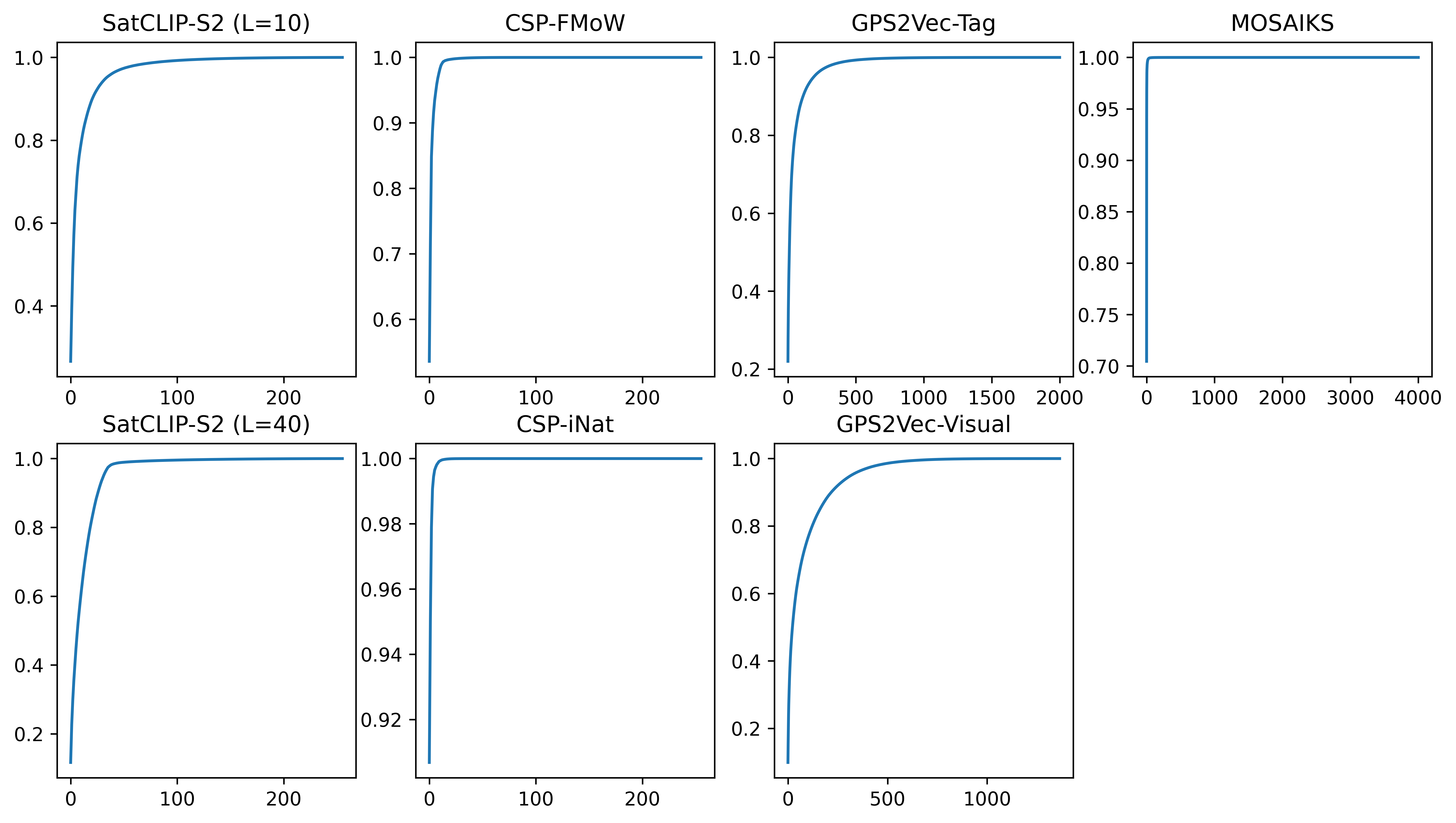
Figure 9: Curves of the explained variance ratio of a principal component analysis (PCA) conducted on the different embeddings using globally distributed locations from the Countries dataset.

Table 4: Description of the datasets used in downstream experiments.

Name	$n$	Spatial coverage	Locations	Outcome variable	Inputs	Task
Air Temp. [9]	$3,076$	Global	Weather stations	Ann. mean temp.	lon, lat	Regr.
Med. Income [14]	$3,107$	Cont., USA	Census tract	Med. house inc.	lon, lat	Regr.
Cali. Housing [28]	$20,640$	Calif., USA	House locations	House price	lon, lat	Regr.
Elev. [32]	$99,995$	Global	Reg. sampled	Elevation	lon, lat	Regr.
Pop. Dens. [32]	$74,512$	Global	Reg. sampled	Pop. dens.	lon, lat	Regr.
Countries (Ours)	$100,000$	Global	Reg. sampled	Country code	lon, lat	Class.
Biome [7]	$100,000$	Global	Reg. sampled	Biome type	lon, lat	Class.
Ecoregions [7]	$100,000$	Global	Reg. sampled	Ecoregion	lon, lat	Class.
iNat 2018 [10]	$460,406$	Global	Image locations	Species classes	lon, lat, image	Class.

Appendix E Experimental details and additional results

E.1 Countries, Ecoregions, and Biome Dataset Overview

To create the Countries, Ecoregions and Biome datasets used in Section 5 we sample a dataset of 100,000 latitude and longitude points approximate uniformly at random, then record which country, ecoregion and biome each point falls within, or whether the point is over an ocean. We use country boundaries from the 4.1 release of “The Database of Global Administrative Areas” (GADM, gadm.org) for country codes. We rely on Dinerstein et al. [7] for ecoregion and biome maps. The Countries dataset contains points over 184 countries (out of a total of 263 countries in the GADM dataset), resulting in a classification task with 185 categories (including an “ocean” class). The Ecoregions dataset contains 719 classes, also including an “ocean” class. The Biome dataset contains 15 classes and also includes an “ocean” class. Note that the latitude/longitude locations for all three datasets are the same.

E.2 Downstream Task Overview

Tab. 4 highlights the different datasets used in downstream tasks throughout our experiments along with characteristics like their spatial coverage, outcome variables and task types. Generally, our tasks can be split into regression and (multi-)classification tasks. Our inputs are always raw longitude/latitude coordinate pairs which are processed by our pretrained location encoders to obtain location embeddings which are then used as inputs for downstream learners. The population density and elevation datasets are subsampled from the global datasets from Rolf et al. [32]. Only the iNat 2018 task contains additional data: image embeddings obtained via a pretrained InceptionV3 network.

E.3 Training details

We tune all downstream task models before final training runs. All reported downstream experiments use simple MLP models. We tune the following hyperparameters by random search: number of hidden layers, hidden dimensions, learning rate, weight decay. The best setting is selected according to a validation loss. We then train $10$ models until convergence (as measured on the validation loss) and report mean and standard deviations of performance metrics (MSE or accuracy). All tuning and training is conducted on a single A100 GPU.

For experiments reported in Sec. 5.1, we deploy random train/val/test splits. For the Air Temp. dataset the training size is $60\%$, for the Cali. Housing and Med. Income datasets it is $50\%$ and for all other datasets it is $30\%$. The validation set size is $20\%$ for Air Temp., Cali. Housing and Med. Income and $10\%$ for all other datasets. Note that the iNat 2018 dataset comes with predefined train and test sets. Here we reserve $10\%$ of the train set for validation. For experiments reported in Sec. 5.2 train and test set are defined by the location of points within or outside of the respective test set continent. Here, we reserve $20\%$ of the training set for validation for Air Temp., Cali. Housing and Med. Income and $10\%$ for all other datasets. For Countries and Ecoregions we allocated a small portion ($1\%$) of test set points for training to allow the models to learn classes that only exist on the test set continent.

E.4 Results of Different SatCLIP Configurations

We provide full experimental results for pretrained SatCLIPs (with different numbers of Legendre polynomials $L$ and different vision backbones ResNet18, ResNet50 and ViT16) in Tab. 6.

E.5 Additional Figures: Predictive Performance

(a) Predictive performance: Country code classification

(b) Prediction errors: Population density.

Figure 10: Fig. 10(a) shows results from the Countries dataset. Shown are predicted country codes across the planet, compared to the true country codes. Fig. 10(b) shows test set results from the Population dataset. Shown are model residuals (errors), red values indicate positive, blue values negative errors. Errors are standardized across figures.

Table 5: Downstream task performance using combinations of different embeddings. We report average test set MSE and accuracy $\pm 1$ standard deviation across $10$ independently initialized MLP training runs. Here, SatCLIP corresponds to a model with $L=10$.

Embedding $1$ Embedding $2$ Air Temp. Med. Income Cali. Housing Elevation Population SatCLIP-RN50 CSP (iNat) $0.0023(\pm 0.0002)$ $0.0108(\pm 0.0003)$ $0.0404(\pm 0.0006)$ $0.0026(\pm 0.0001)$ $0.0069(\pm 0.0002)$ SatCLIP-RN50 GPS2Vec (tag) $0.0026(\pm 0.0002)$ $0.0095(\pm 0.0002)$ $0.0376(\pm 0.0006)$ $0.0022(\pm 0.0001)$ $0.006(\pm 0.0001)$ SatCLIP-RN50 GPS2Vec (visual) $0.0031(\pm 0.0002)$ $0.0097(\pm 0.0002)$ $0.0382(\pm 0.001)$ $0.0024(\pm 0.0002)$ $0.0061(\pm 0.0001)$ CSP (iNat) GPS2Vec (tag) $0.0156(\pm 0.0008)$ $0.0129(\pm 0.0002)$ $0.0566(\pm 0.0009)$ $0.0088(\pm 0.0004)$ $0.0206(\pm 0.0016)$ CSP (iNat) GPS2Vec (visual) $0.0185(\pm 0.0022)$ $0.013(\pm 0.0001)$ $0.0572(\pm 0.0007)$ $0.0091(\pm 0.0002)$ $0.0178(\pm 0.0004)$ GPS2Vec (visual) GPS2Vec (tag) $0.0299(\pm 0.0018)$ $0.0119(\pm 0.0002)$ $0.0253(\pm 0.0013)$ $0.009(\pm 0.0)$ $0.0203(\pm 0.0001)$

Fig. 10 shows results (signed errors) for air temperature, population density and country code prediction, where the improvements from SatCLIP are visually apparent. Tab. 2 shows test set results on all datasets. One interesting observation is that this use of SatCLIP embeddings are more informative for iNat classification than a location encoder pretrained on iNat (CSP-iNat). This is intuitive as SatCLIP embeddings might be able to provide auxiliary information not contained within the iNat imagery. Overall, the results confirm that SatCLIP models trained on SK-100K data provide meaningful features to help with prediction in both natural (e.g., Air Temp., Elevation) and socio-economic (e.g., Med. Income, Cali. Housing) settings.

E.6 Additional Figures: Geographic Generalization

Figure 11: Few-shot ecoregion prediction. Predictions on the test continent Africa are shown for the different embeddings. Models are trained on only $1\%$ of the data points on the test continent to evaluate their capacity for generalizing to an unseen environment.

Fig. 11 shows results for the few-shot domain generalization setting with the Ecoregions dataset. Here, we highlight true values and predictions on the test set continent Africa. We can see that SatCLIP embeddings perform best, followed by MOSAIKS embeddings. This experiment helps us to evaluate the embeddings capacity for overcoming geographic distribution shift.

E.7 Additional Results: Combining Embeddings

We test whether combinations of embeddings obtained from location encoders trained on different datasets further improves performance. We do this by concatenating the embeddings before feeding them to the downstream learner. We show in our results in Tab. 5 that combinations do not help and performance is not improved.

Table 6: SatCLIP models with different vision encoders and location encoders win varying resolutions controlled by the L parameter (maximum number of Legendre polynomial degrees). We report average test set MSE and accuracy $\pm 1$ standard deviation across $10$ independently initialized MLP training runs.

(a) Classification Accuracy in % and Regression MSE to extend Tab. 2

Vision Encoder	ViT16	ViT16	ResNet18	ResNet18	ResNet50	ResNet50
Spherical Harm. $L$	10	40	10	40	10	40
Regression MSE $\downarrow$
Air Temp.	$\mathbf{0.20\pm 0.31}$	$0.25\pm 0.02$	$0.59\pm 0.75$	$0.81\pm 0.77$	$0.29\pm 0.38$	$0.27\pm 0.03$
Median Income	$0.92\pm 0.24$	$\mathbf{0.67\pm 0.01}$	$0.87\pm 0.22$	$\mathbf{0.67\pm 0.01}$	$0.78\pm 0.02$	$0.71\pm 0.16$
Cali Housing	$3.55\pm 0.06$	$2.62\pm 0.28$	$3.66\pm 0.13$	$\mathbf{2.46\pm 0.08}$	$3.68\pm 0.23$	$\mathbf{2.42\pm 0.12}$
Elevation	$0.22\pm 0.01$	$\mathbf{0.15\pm 0.01}$	$0.20\pm 0.01$	$\mathbf{0.15\pm 0.00}$	$0.21\pm 0.01$	$\mathbf{0.15\pm 0.00}$
Population Density	$0.56\pm 0.01$	$0.50\pm 0.02$	$0.55\pm 0.01$	$\mathbf{0.48\pm 0.01}$	$0.55\pm 0.01$	$\mathbf{0.48\pm 0.01}$
Classification % Acc. $\uparrow$
Countries	$93.97\pm 0.30$	$95.77\pm 0.14$	$93.92\pm 0.30$	$95.92\pm 0.10$	$94.28\pm 0.18$	$\mathbf{96.00\pm 0.14}$
iNaturalist	$65.69\pm 0.50$	${65.98\pm 0.61}$	$65.56\pm 0.29$	$\mathbf{66.40\pm 0.49}$	$65.50\pm 0.43$	${66.03\pm 0.54}$
Biomes	$92.07\pm 0.22$	$\mathbf{94.27\pm 0.15}$	$92.10\pm 0.23$	$\mathbf{94.33\pm 0.10}$	$92.23\pm 0.26$	$\mathbf{94.41\pm 0.14}$
Ecoregions	$89.53\pm 0.28$	$\mathbf{91.61\pm 0.22}$	$89.57\pm 0.23$	$\mathbf{91.53\pm 0.15}$	$89.32\pm 0.31$	$\mathbf{91.67\pm 0.15}$

(b) Held-out countries regression and classification tasks. This table extends Tab. 3

Vision Encoder	ViT16	ViT16	ResNet18	ResNet18	ResNet50	ResNet50
Spherical Harm. $L$	10	40	10	40	10	40
Asia
Air Temp.∗ MSE $\downarrow$	$\mathbf{0.85\pm 0.17}$	$1.26\pm 0.15$	$1.22\pm 0.56$	$1.56\pm 0.14$	$1.17\pm 0.52$	$1.50\pm 0.10$
Elevation∗	$2.13\pm 0.37$	$\mathbf{2.06}\pm 0.28$	$2.36\pm 0.21$	$2.58\pm 0.26$	$2.22\pm 0.35$	$3.28\pm 0.09$
Population Density∗	$2.03\pm 0.26$	$\mathbf{1.94\pm 0.15}$	$2.18\pm 0.21$	$\mathbf{1.92\pm 0.23}$	$2.06\pm 0.21$	$2.82\pm 0.22$
Countries† % Acc. $\uparrow$	$36.90\pm 4.32$	$19.17\pm 2.82$	$37.15\pm 3.28$	$13.71\pm 3.26$	$\mathbf{40.36\pm 3.21}$	$14.29\pm 1.62$
iNaturalist∗	$19.60\pm 0.78$	$\mathbf{20.91\pm 0.77}$	$\mathbf{20.75\pm 1.00}$	$19.67\pm 0.97$	$19.75\pm 0.49$	$17.67\pm 0.32$
Biome∗	$25.89\pm 2.79$	$16.44\pm 1.21$	$21.97\pm 3.50$	$15.02\pm 0.97$	$21.83\pm 3.44$	$\mathbf{30.26\pm 3.00}$
Ecoregions†	$\mathbf{21.02\pm 1.09}$	$10.86\pm 1.19$	$\mathbf{20.54\pm 1.55}$	$8.87\pm 1.70$	$\mathbf{20.32\pm 1.41}$	$8.46\pm 0.79$
Africa
Air Temp.∗ MSE $\downarrow$	$4.13\pm 1.66$	$\mathbf{1.79\pm 0.50}$	$3.36\pm 0.91$	$17.60\pm 25.27$	$6.56\pm 1.53$	$2.17\pm 0.33$
Elevation∗	$1.34\pm 0.83$	$\mathbf{0.57\pm 0.04}$	$1.25\pm 0.36$	$0.73\pm 0.05$	$1.41\pm 0.51$	$0.81\pm 0.06$
Pop. D.∗	$\mathbf{1.97\pm 0.29}$	$\mathbf{1.96\pm 0.22}$	$2.39\pm 0.46$	$2.14\pm 0.25$	$2.63\pm 0.50$	$2.99\pm 0.23$
Countries† % Acc. $\uparrow$	$30.65\pm 4.23$	$10.22\pm 1.62$	$\mathbf{34.41\pm 3.18}$	$9.96\pm 1.56$	$\mathbf{35.30\pm 2.00}$	$8.95\pm 1.04$
iNaturalist∗	$9.53\pm 0.57$	$6.23\pm 0.47$	$8.96\pm 0.88$	$6.68\pm 0.44$	$\mathbf{9.90\pm 0.52}$	$5.22\pm 0.26$
Biome∗	$35.72\pm 5.48$	$12.34\pm 1.75$	$34.58\pm 5.14$	$20.60\pm 1.40$	$\mathbf{39.93\pm 4.41}$	$33.77\pm 2.69$
Ecoregions†	$\mathbf{32.03\pm 1.19}$	$12.91\pm 1.63$	$\mathbf{31.66\pm 2.29}$	$12.87\pm 2.47$	$\mathbf{32.69\pm 1.79}$	$13.54\pm 2.06$
∗ Denotes zero-shot, † denotes few-shot domain generalization tasks.

References

- Beery et al. [2022] Sara Beery, Guanhang Wu, Trevor Edwards, Filip Pavetic, Bo Majewski, Shreyasee Mukherjee, Stanley Chan, John Morgan, Vivek Rathod, and Jonathan Huang. The auto arborist dataset: A large-scale benchmark for multiview urban forest monitoring under domain shift. In Proceedings of the IEEE Computer Society Conference on Computer Vision and Pattern Recognition (CVPR), pages 21294–21307, 2022.
- Carleton et al. [2022] Tamma Carleton, Trinetta Chong, Hannah Druckenmiller, Eugenio Noda, Jonathan Proctor, Esther Rolf, and Solomon Hsiang. Multi-Task Observation Using Satellite Imagery and Kitchen Sinks (MOSAIKS) API. https://siml.berkeley.edu, 2022.
- Cepeda et al. [2023] Vicente Vivanco Cepeda, Gaurav Kumar Nayak, and Mubarak Shah. Geoclip: Clip-inspired alignment between locations and images for effective worldwide geo-localization. arXiv preprint arXiv:2309.16020, 2023.
- Chen et al. [2019] Cen Chen, Kenli Li, Sin G. Teo, Xiaofeng Zou, Kang Wang, Jie Wang, and Zeng Zeng. Gated residual recurrent graph neural networks for traffic prediction. In Proceedings of the AAAI Conference on Artificial Intelligence, pages 485–492. AAAI Press, 2019.
- Christie et al. [2018] Gordon Christie, Neil Fendley, James Wilson, and Ryan Mukherjee. Functional map of the world. In Proceedings of the IEEE Computer Society Conference on Computer Vision and Pattern Recognition (CVPR), pages 6172–6180, 2018.
- Cole et al. [2023] Elijah Cole, Grant Van Horn, Christian Lange, Alexander Shepard, Patrick Leary, Pietro Perona, Scott Loarie, and Oisin Mac Aodha. Spatial implicit neural representations for global-scale species mapping. In Proceedings of the 40th International Conference on Machine Learning, pages 6320–6342. PMLR, 2023.
- Dinerstein et al. [2017] Eric Dinerstein, David Olson, Anup Joshi, Carly Vynne, Neil D Burgess, Eric Wikramanayake, Nathan Hahn, Suzanne Palminteri, Prashant Hedao, Reed Noss, et al. An ecoregion-based approach to protecting half the terrestrial realm. BioScience, 67(6):534–545, 2017.
- He et al. [2020] Kaiming He, Haoqi Fan, Yuxin Wu, Saining Xie, and Ross Girshick. Momentum contrast for unsupervised visual representation learning. In Proceedings of the IEEE/CVF conference on computer vision and pattern recognition, pages 9729–9738, 2020.
- Hooker et al. [2018] Josh Hooker, Gregory Duveiller, and Alessandro Cescatti. Data descriptor: A global dataset of air temperature derived from satellite remote sensing and weather stations. Scientific Data, 5:1–11, 2018.
- Horn et al. [2018] Grant Van Horn, Oisin Mac Aodha, Yang Song, Yin Cui, Chen Sun, Alex Shepard, Hartwig Adam, Pietro Perona, Serge Belongie, Caltech 2 Google, and Cornell Tech. The iNaturalist species classification and detection dataset. In Proceedings of the IEEE Computer Society Conference on Computer Vision and Pattern Recognition (CVPR), pages 8769–8778, 2018.
- Hu et al. [2019] Wenjie Hu, Jay Harshadbhai Patel, Zoe-Alanah Robert, Paul Novosad, Samuel Asher, Zhongyi Tang, Marshall Burke, David Lobell, and Stefano Ermon. Mapping missing population in rural India: A deep learning approach with satellite imagery. In Proceedings of the AAAI Conference on Artificial Intelligence, 2019.
- Jean et al. [2016] Neal Jean, Marshall Burke, Michael Xie, W Matthew Davis, David B Lobell, and Stefano Ermon. Combining satellite imagery and machine learning to predict poverty. Science, 353:790–794, 2016.
- Jean et al. [2019] Neal Jean, Sherrie Wang, Anshul Samar, George Azzari, David Lobell, and Stefano Ermon. Tile2vec: Unsupervised representation learning for spatially distributed data. In Proceedings of the AAAI Conference on Artificial Intelligence, 2019.
- Jia and Benson [2020] Junteng Jia and Austion R. Benson. Residual correlation in graph neural network regression. In Proceedings of the ACM SIGKDD International Conference on Knowledge Discovery and Data Mining, pages 588–598. Association for Computing Machinery, 2020.
- Kingma and Ba [2015] Diederik P Kingma and Jimmy Lei Ba. Adam: A method for stochastic optimization. In Proceedings in the International Conference on Learning Representations (ICLR), 2015.
- Klemmer and Neill [2021] Konstantin Klemmer and Daniel B. Neill. Auxiliary-task learning for geographic data with autoregressive embeddings. In SIGSPATIAL: Proceedings of the ACM International Symposium on Advances in Geographic Information Systems, 2021.
- Klemmer et al. [2020] Konstantin Klemmer, Godwin Yeboah, João Porto de Albuquerque, and Stephen A Jarvis. Population mapping in informal settlements with high-resolution satellite imagery and equitable ground-truth. 2020.
- Klemmer et al. [2022] Konstantin Klemmer, Tianlin Xu, Beatrice Acciaio, and Daniel B. Neill. Spate-gan: Improved generative modeling of dynamic spatio-temporal patterns with an autoregressive embedding loss. Proceedings of the AAAI Conference on Artificial Intelligence, 36:4523–4531, 2022.
- Kondmann et al. [2021] Lukas Kondmann, Aysim Toker, Marc Rußwurm, Andrés Camero, Devis Peressuti, Grega Milcinski, Pierre-Philippe Mathieu, Nicolas Longépé, Timothy Davis, Giovanni Marchisio, et al. Denethor: The dynamicearthnet dataset for harmonized, inter-operable, analysis-ready, daily crop monitoring from space. In Thirty-fifth Conference on Neural Information Processing Systems Datasets and Benchmarks Track (Round 2), 2021.
- Lacoste et al. [2023] Alexandre Lacoste, Nils Lehmann, Pau Rodriguez, Evan David Sherwin, Hannah Kerner, Björn Lütjens, Jeremy Andrew Irvin, David Dao, Hamed Alemohammad, Alexandre Drouin, Mehmet Gunturkun, Gabriel Huang, David Vazquez, Dava Newman, Yoshua Bengio, Stefano Ermon, and Xiao Xiang Zhu. Geo-bench: Toward foundation models for earth monitoring. arXiv preprint arXiv:2306.03831, 2023.
- Larson et al. [2017] Martha Larson, Mohammad Soleymani, Guillaume Gravier, Bogdan Ionescu, and Gareth J.F. Jones. The benchmarking initiative for multimedia evaluation: Mediaeval 2016. IEEE Multimedia, 24:93–96, 2017.
- Lobell et al. [2015] David B Lobell, David Thau, Christopher Seifert, Eric Engle, and Bertis Little. A scalable satellite-based crop yield mapper. Remote Sensing of Environment, 164:324–333, 2015.
- Loos and Niemann [2002] Eduardo A. Loos and K. Olaf Niemann. Shoreline feature extraction from remotely-sensed imagery. International Geoscience and Remote Sensing Symposium (IGARSS), 6:3417–3419, 2002.
- Mac Aodha et al. [2019] Oisin Mac Aodha, Elijah Cole, and Pietro Perona. Presence-only geographical priors for fine-grained image classification. In ICCV, 2019.
- Mai et al. [2020] Gengchen Mai, Krzysztof Janowicz, Bo Yan, Rui Zhu, Ling Cai, and Ni Lao. Multi-scale representation learning for spatial feature distributions using grid cells. In Proceedings in the International Conference on Learning Representations (ICLR), 2020.
- Mai et al. [2023] Gengchen Mai, Ni Lao, Yutong He, Jiaming Song, and Stefano Ermon. CSP: Self-supervised contrastive spatial pre-training for geospatial-visual representations. arXiv preprint arXiv:2305.01118, 2023.
- Mañas et al. [2021] Oscar Mañas, Alexandre Lacoste, Xavier Giró i Nieto, David Vazquez, and Pau Rodríguez. Seasonal contrast: Unsupervised pre-training from uncurated remote sensing data. In Proceedings of the IEEE Computer Society Conference on Computer Vision and Pattern Recognition (CVPR), pages 9414–9423, 2021.
- Pace and Barry [2003] R. Kelley Pace and Ronald Barry. Sparse spatial autoregressions. Statistics & Probability Letters, 33:291–297, 2003.
- Quackenbush [2004] Lindi J. Quackenbush. A review of techniques for extracting linear features from imagery. Photogrammetric Engineering and Remote Sensing, 70:1383–1392, 2004.
- Radford et al. [2021] Alec Radford, Jong Wook Kim, Chris Hallacy, Aditya Ramesh, Gabriel Goh, Sandhini Agarwal, Girish Sastry, Amanda Askell, Pamela Mishkin, Jack Clark, Gretchen Krueger, and Ilya Sutskever. Learning transferable visual models from natural language supervision. In Proceedings in the International Conference on Machine Learning (ICML), pages 8748–8763. PMLR, 2021.
- Reiersen et al. [2022] Gyri Reiersen, David Dao, Björn Lütjens, Konstantin Klemmer, Kenza Amara, Attila Steinegger, Ce Zhang, and Xiaoxiang Zhu. Reforestree: A dataset for estimating tropical forest carbon stock with deep learning and aerial imagery. Proceedings of the AAAI Conference on Artificial Intelligence, 36:12119–12125, 2022.
- Rolf et al. [2021] Esther Rolf, Jonathan Proctor, Tamma Carleton, Ian Bolliger, Vaishaal Shankar, Miyabi Ishihara, Benjamin Recht, and Solomon Hsiang. A generalizable and accessible approach to machine learning with global satellite imagery. Nature Communications 2021 12:1, 12:1–11, 2021.
- Rußwurm et al. [2020] Marc Rußwurm, Sherrie Wang, Marco Korner, and David Lobell. Meta-learning for few-shot land cover classification. In Proceedings of the ieee/cvf conference on computer vision and pattern recognition workshops, pages 200–201, 2020.
- Rußwurm et al. [2023] Marc Rußwurm, Konstantin Klemmer, Esther Rolf, Robin Zbinden, and Devis Tuia. Geographic location encoding with spherical harmonics and sinusoidal representation networks. arXiv preprint arXiv:2310.06743, 2023.
- Scheibenreif et al. [2022] Linus Scheibenreif, Joëlle Hanna, Michael Mommert, and Damian Borth. Self-supervised vision transformers for land-cover segmentation and classification. In Proceedings of the IEEE/CVF Conference on Computer Vision and Pattern Recognition, pages 1422–1431, 2022.
- Sitzmann et al. [2020] Vincent Sitzmann, Julien N P Martel, Alexander W Bergman, David B Lindell, and Gordon Wetzstein. Implicit neural representations with periodic activation functions. Advances in Neural Information Processing Systems, 33:7462–7473, 2020.
- Thomee et al. [2016] Bart Thomee, Benjamin Elizalde, David A. Shamma, Karl Ni, Gerald Friedland, Douglas Poland, Damian Borth, and Li Jia Li. YFCC100M. Communications of the ACM, 59:64–73, 2016.
- Tiede et al. [2021] Dirk Tiede, Gina Schwendemann, Ahmad Alobaidi, Lorenz Wendt, and Stefan Lang. Mask R-CNN-based building extraction from VHR satellite data in operational humanitarian action: An example related to Covid-19 response in Khartoum, Sudan. Transactions in GIS, 25:1213–1227, 2021.
- Tseng et al. [2022] Gabriel Tseng, Hannah Kerner, and David Rolnick. TIML: Task-informed meta-learning for agriculture. arXiv preprint arXiv:2202.02124, 2022.
- Van der Maaten and Hinton [2008] Laurens Van der Maaten and Geoffrey Hinton. Visualizing data using t-SNE. Journal of machine learning research, 9(11), 2008.
- Wang et al. [2022a] Yi Wang, Nassim Ait, Ali Braham, Zhitong Xiong, Chenying Liu, Conrad M Albrecht, and Xiao Xiang Zhu. SSL4EO-S12: A large-scale multi-modal, multi-temporal dataset for self-supervised learning in Earth observation. 2022a.
- Wang et al. [2022b] Yi Wang, Conrad M. Albrecht, Nassim Ait Ali Braham, Lichao Mou, and Xiao Xiang Zhu. Self-supervised learning in remote sensing: A review. IEEE Geoscience and Remote Sensing Magazine, 10:213–247, 2022b.
- Willing et al. [2017] Christoph Willing, Konstantin Klemmer, Tobias Brandt, and Dirk Neumann. Moving in time and space – location intelligence for carsharing decision support. Decision Support Systems, 2017.
- Wurm et al. [2019] Michael Wurm, Thomas Stark, Xiao Xiang Zhu, Matthias Weigand, and Hannes Taubenböck. Semantic segmentation of slums in satellite images using transfer learning on fully convolutional neural networks. ISPRS Journal of Photogrammetry and Remote Sensing, 150:59–69, 2019.
- Yin et al. [2019] Yifang Yin, Zhenguang Liu, Ying Zhang, Sheng Wang, Rajiv Ratn Shah, and Roger Zimmermann. GPS2Vec: Towards generating worldwide GPS embeddings. In SIGSPATIAL: Proceedings of the ACM International Symposium on Advances in Geographic Information Systems, pages 416–419. Association for Computing Machinery, 2019.
- Zhai et al. [2023] Xiaohua Zhai, Basil Mustafa, Alexander Kolesnikov, Lucas Beyer, and Google Deepmind. Sigmoid loss for language image pre-training. In ICCV, 2023.
- Zhan et al. [2007] Qingming Zhan, Martien Molenaar, Klaus Tempfli, and Wenzhong Shi. Quality assessment for geo‐spatial objects derived from remotely sensed data. International Journal of Remote Sensing, 26:2953–2974, 2007.