Robust Diffusion GAN using Semi-Unbalanced Optimal Transport

Abstract

Diffusion models, a type of generative model, have demonstrated great potential for synthesizing highly detailed images. By integrating with GAN, advanced diffusion models like DDGAN [51] could approach real-time performance for expansive practical applications. While DDGAN has effectively addressed the challenges of generative modeling, namely producing high-quality samples, covering different data modes, and achieving faster sampling, it remains susceptible to performance drops caused by datasets that are corrupted with outlier samples. This work introduces a robust training technique based on semi-unbalanced optimal transport to mitigate the impact of outliers effectively. Through comprehensive evaluations, we demonstrate that our robust diffusion GAN (RDGAN) outperforms vanilla DDGAN in terms of the aforementioned generative modeling criteria, i.e., image quality, mode coverage of distribution, and inference speed, and exhibits improved robustness when dealing with both clean and corrupted datasets.

1 Introduction

Despite their relatively recent introduction, diffusion models have experienced rapid growth and garnered significant attention in the research community. These models effectively reverse the diffusion process from Gaussian random noise inputs into clean, high-quality images. The models have found utility across diverse data domains, with their most remarkable successes being in the realm of image generation. Notably, diffusion models outperform state-of-the-art generative adversarial networks (GANs) in terms of quality of generated content on various datasets, as shown in [9, 40]. Furthermore, they exhibit superior mode coverage, as discovered by [44, 15, 21], and offer adaptability in handling a wide range of conditional inputs, including semantic maps, text and images, as highlighted in the work of [37, 30, 49]. This flexibility has led to their application in various areas, such as text-to-image generation, image-to-image translation, image inpainting, image restoration, and more. Recent advancements in text-to-image generative models, based on diffusion techniques as proposed by [36, 40], have enabled the generation of highly realistic images from textual inputs. Furthermore, personalized text-to-image diffusion models, such as [39, 26], have found extensive applications in various real-world scenarios.

Nonetheless, despite their immense potential, diffusion models are hindered by a significant weakness: their slow sampling speed. This limitation prevents their widespread adoption, contrasting them with GANs. The foundational Denoising Diffusion Probabilistic Models (DDPMs) by [14] require a thousand sampling steps to attain the desired output quality, resulting in minutes of computation for a single image generation. Although several techniques have been devised to reduce inference time [43, 29, 52], primarily through the reduction of sampling steps, they still take seconds to generate a 32$\times$32 image—roughly 100 times slower than GANs. Diffusion GAN (DDGAN), as introduced by [51], has effectively tackled the challenge of modeling complex multimodal distributions, particularly when dealing with large step sizes, through the utilization of generative adversarial networks. This innovative approach has led to a significant reduction in the number of denoising steps required, typically just a few (e.g., 2 or 4). Consequently, inference time has been drastically reduced to mere fractions of a second.

In practice, datasets collected unintentionally inevitably contain outliers during the data collection process. These outliers can significantly harm the performance of generative models. However, because of the dataset’s large scale, removing these outlier samples can be a daunting and time-consuming task. As a result, there is a strong demand for developing robust generative models that can counteract the negative effects of noisy datasets. While DDGAN has succeeded in striking a good balance among three crucial aspects of generative models—mode coverage, high-resolution synthesis, and fast sampling—we have observed a notable decline in DDGAN’s performance when it encounters noisy data containing outliers. This limitation hinders its practical application. Given that DDGAN comprises multiple GAN models between two consecutive timesteps, we delve into the evolution of GANs to find a solution to the noise problem. Before the diffusion era, Generative Adversarial Networks (GANs) were the dominant generative model type extensively studied and utilized in real-world applications. Simultaneously, the application of Optimal Transport theory [48], specifically Wasserstein distance, played a pivotal role in addressing key issues in generative models. This included enhancing diversity [2, 12], improving convergence [41], and ensuring stability [31] in GANs. To address the challenge posed by noisy datasets, several research efforts have incorporated Unbalanced Optimal Transport formulations [5] into the GAN, successfully reducing the impact of outliers in image synthesis [3, 6, 33].

Inspired by the Unbalanced Optimal Transport theory [5], we introduced RDGAN, which relies on semi-unbalanced optimal transport, as a solution to the noisy dataset problem. Our approach reformulates the adversarial training between two consecutive diffusion timesteps based on the semi-unbalanced optimal transport formulation, thereby relaxing the strict marginal constraints. Through extensive experiments, we demonstrate that our proposed method, RDGAN, not only maintains a good Fréchet Inception Distance (FID) score [13], a key metric for assessing image quality but also achieves rapid training convergence compared to the standard DDGAN. Furthermore, we successfully mitigate the impact of corrupted samples in noisy training datasets. In summary, our research has led to several noteworthy contributions:

• Enhanced Robustness: Firstly, we’ve identified a key limitation of DDGAN when confronted with noisy datasets that include outliers. To overcome this challenge, we introduce Robust Diffusion GAN (RDGAN), a novel approach that demonstrates remarkable resilience under the presence of outliers.

• Superior Image Generation: Not only robust to outliers, RDGAN also generates images at higher quality compared to the baseline DDGAN on either clean or corrupted datasets, which is consistently confirmed via extensive experiments with both FID and Recall metrics.

• Improved Training Convergence: Expanding upon its image generation capabilities, RDGAN also introduces substantial enhancements in training stability, surpassing its predecessor, DDGAN. This heightened stability serves to optimize the training pipeline, rendering it both more dependable and operationally efficient.

2 Background

2.1 Diffusion Models

Diffusion models that rely on the diffusion process often take empirically thousand steps to diffuse the original data to become a neat approximation of Gaussian noise. Let’s use $x_{0}$ to denote the true data, and $x_{t}$ denotes that datum after $t$ steps of rescaling data and adding Gaussian noise. The probability distributions of $x_{t}$ conditioned on $x_{t-1}$ and $x_{0}$ has the form

$$q(x_{t}|x_{t-1}) =\mathcal{N}(\sqrt{1-\beta_{t}}x_{t-1},\beta_{t}\mathbf{I})$$ (1)

$$q(x_{t}|x_{0}) =\mathcal{N}(x_{t};\sqrt{\overline{\alpha}_{t}}x_{0},(1-\overline{\alpha}_{t})\mathbf{I})$$ (2)

where $\alpha_{t}=1-\beta_{t}$, $\bar{\alpha_{t}}=\prod_{s=1}^{t}\alpha_{s}$, and $\beta_{t}\in(0,1)$ is set to be relatively small, either through a learnable schedule or as a fixed value at each time step in the forward process. Given that the diffusion process introduces relatively minor noise with each step, we can estimate the reverse process, denoted as $q(x_{t-1}|x_{t})$, by using a Gaussian process, specifically, $q(x_{t-1}|x_{t},x_{0})$, which in turn could be learned through a parameterized function $p_{\theta}(x_{t-1}|x_{t})$. Following [14], $p_{\theta}(x_{t-1}|x_{t})$ is commonly parameterized as:

$$p_{\theta}(x_{t-1}\mid x_{t})=\mathcal{N}(x_{t-1};\mu_{\theta}(x_{t},t),\sigma^{2}_{t}\mathbf{I}),$$ (3)

where $\mu_{\theta}(x_{t},t)$ and $\sigma^{2}_{t}$ represent the mean and variance of parameterized denoising model, respectively. The learning objective is to minimize the Kullback-Leibler (KL) divergence between the true denoising distribution $q(x_{t-1}|x_{t})$ and the denoising distribution parameterized by $p_{\theta}(x_{t-1}|x_{t})$.

Unlike traditional diffusion methods, DDGAN [51] allows for larger denoising step sizes to speed up the sampling process by incorporating generative adversarial networks (GANs). DDGAN introduces a discriminator, denoted as $D_{\phi}$, and optimizes both the generator and discriminator in an adversarial training fashion. The objective of DDGAN can be expressed as follows:

$$\min_{\phi}\max_{\theta} \sum_{t\geq 1}\mathbb{E}_{q\left(\mathbf{x}_{t}\right)}\bigg{\{}\mathbb{E}_{q\left(\mathbf{x}_{t-1}\mid\mathbf{x}_{t}\right)}\Big{[}-\log\big{(}D_{\phi}(\mathbf{x}_{t-1},\mathbf{x}_{t},t)\big{)}\Big{]}$$

$$+\mathbb{E}_{p_{\theta}\left(\mathbf{x}_{t-1}\mid\mathbf{x}_{t}\right)}\Big{[}\log\big{(}D_{\phi}(\mathbf{x}_{t-1},\mathbf{x}_{t},t)\big{)}\Big{]}\bigg{\}}$$ (4)

In Eq. 4, fake samples are generated from a conditional generator $p_{\theta}(x_{t-1}|x_{t})$. Due to the use of large step sizes, the distribution $q(x_{t-1}|x_{t})$ is no longer Gaussian. DDGAN addresses this by implicitly modeling this complex multimodal distribution using a generator $G_{\theta}(x_{t},z,t)$, where $z$ is a $D$-dimensional latent variable drawn from a standard Gaussian distribution $\mathcal{N}(0,\mathbf{I})$. Specifically, DDGAN first generates an unperturbed sample $x_{0}^{\prime}$ through the generator $G_{\theta}(x_{t},z,t)$ and obtains the corresponding perturbed sample $x_{t-1}^{\prime}$ using $q(x_{t-1}|x_{t},x_{0})$. Simultaneously, the discriminator evaluates both real pairs $D_{\phi}(x_{t-1},x_{t},t)$ and fake pairs $D_{\phi}(x_{t-1}^{\prime},x_{t},t)$ to guide the training process.

2.2 Unbalanced Optimal Transport

In this section, we provide some background on optimal transport (OT), its unbalanced formulation (UOT), and their applications.

Optimal Transport: Let $\mu$ and $\nu$ be two probability measures in the set of probability measures ${\mathcal{P}}({\mathcal{X}})$ for space ${\mathcal{X}}$, the OT distance between $\mu$ and $\nu$ is defined as:

$$\mathsf{OT}(\mu,\nu)=\min_{\pi\in\Pi(\mu,\nu)}\int c(x,y)d\pi(x,y),$$ (5)

where $c:{\mathcal{X}}\times{\mathcal{X}}\rightarrow[0,\infty)$ is a cost function, $\Pi(\mu,\nu)$ is the set of joint probability measures on ${\mathcal{X}}\times{\mathcal{X}}$ which has $\mu$ and $\nu$ as marginal probability measures. The dual form of OT is:

$$\mathsf{OT}(\mu,\nu) =\sup_{u(x)+v(y)\leq c(x,y)}\int_{{\mathcal{X}}}u(x)d\mu(x)$$

$$+\int_{{\mathcal{X}}}v(y)d\nu(y)$$ (6)

Denote $v^{c}(y)=\inf_{y\in{\mathcal{X}}}\big{\{}c(x,y)-v(y)\big{\}}$ to be the $c$-transform of $v(y)$, then the dual formulation of OT could be written in the following form:

$$\mathsf{OT}(\mu,\nu)=\sup_{v}\int_{{\mathcal{X}}}v^{c}(x)d\mu(x)+\int_{{\mathcal{X}}}v(y)d\nu(y).$$

Unbalanced Optimal Transport: A more generalized version of OT introduced by [5] is Unbalanced Optimal Transport (UOT) formulated as follows:

$$\mathsf{UOT}(\mu,\nu) =\min_{\pi\in{\mathcal{M}}({\mathcal{X}}\times{\mathcal{X}})}\int c(x,y)d\pi(x,y)$$

$$+\mathsf{D}_{\Psi_{1}}(\pi_{1}\|\mu)+\mathsf{D}_{\Psi_{2}}(\pi_{2}\|\nu),$$ (7)

where ${\mathcal{M}}({\mathcal{X}}\times{\mathcal{X}})$ denotes the set of joint non-negative measures on ${\mathcal{X}}\times{\mathcal{X}}$; $\pi$ is an element of ${\mathcal{M}}({\mathcal{X}}\times{\mathcal{X}})$, its marginal measures corresponding to $\mu$ and $\nu$ are $\pi_{1}$ and $\pi_{2}$, respectively; the $\mathsf{D}_{\Psi_{i}}$ are often set as the Csiszár-divergence, i.e., Kullback-Leibler divergence, $\chi^{2}$ divergence. In contrast to OT, the UOT does not require hard constraints on the marginal distributions, thus allowing more flexibility to adapt to different situations. The formulation in Eq. 7 has been applied to unbalanced measures to find developmental trajectories of cells [42]. Another application of UOT is robust optimal transport in cases when data are corrupted with outliers [3] or when mini-batch samples [20, 32] are biased representations of the data distribution. Similar to the OT, solving the UOT again could be done through its dual form [5, 11, 46]

$$\mathsf{UOT}(\mu,\nu) =\sup_{u(x)+v(y)\leq c(x,y)}\int_{\mathcal{X}}-\Psi_{1}^{*}(-u(x))d\mu(x)$$

$$+\int_{\mathcal{X}}-\Psi_{2}^{*}(-v(y))d\nu(y),$$ (8)

where $u,v\in\mathcal{C}(\mathcal{X})$ in which $\mathcal{C}$ denotes a set of continuous functions over its domain; $\Psi_{1}^{*}$ and $\Psi_{2}^{*}$ are the convex conjugate functions of $\Psi_{1}$ and $\Psi_{2}$, respectively. If both function $\Psi_{1}^{*}$ and $\Psi_{2}^{*}$ are non-decreasing and differentiable, we could next remove the condition $u(x)+v(y)\leq c(x,y)$ by the $c$-transform for function $v$ to obtain the semi-dual UOT form [46], $v$ is 1-Lipschitz:

$$\mathsf{UOT}(\mu,\nu) =\sup_{||v||_{L}\leq 1}\int_{{\mathcal{X}}}-\Psi_{1}^{*}\big{(}-v^{c}(x)\big{)}d\mu(x)$$

$$+\int_{{\mathcal{X}}}-\Psi_{2}^{*}\big{(}-v(y)\big{)}d\nu(y)$$ (9)

3 Method

In this section, we introduce our framework RDGAN, starting with Denoising Diffusion GAN (DDGAN) [51], a hybrid approach that combines elements of GAN and DDPM. DDGAN is the first model that satisfies all three generative criteria including fast sampling, mode coverage and high-fidelity generation. However, DDGAN is susceptible to outlier samples in noisy datasets, an issue that has been illustrated through a simple toy experiment in Fig. 2. The top-left subfigure in Fig. 2 highlights how DDGAN inadvertently generates outlier samples when trained on noisy datasets. Remarkably, this challenge has remained unaddressed by prior research efforts.

3.1 Robust Diffusion GAN

DDGAN training involves matching the conditional GAN generator $p_{\theta}(x_{t-1}|x_{t})$ and $q(x_{t-1}|x_{t})$ using an adversarial loss that minimizes a divergence $D_{\mathrm{adv}}$ per denoising step.

$$\min_{\theta}\sum_{t\geq 1}\mathbb{E}_{q\left(x_{t}\right)}D_{\mathrm{adv}}\left(q\left(x_{t-1}\mid x_{t}\right)\|p_{\theta}\left(x_{t-1}\mid x_{t}\right)\right)$$ (10)

where $q(x_{t-1}|x_{t})$ is ground truth conditional distribution with $x_{t-1}$ sampling from Eq. 2 and $x_{t}$ sampling from Eq. 1. The fake conditional pair $(\widehat{x}_{t-1},x_{t})\sim p_{\theta}(x_{t-1}|x_{t})$ is obtained using ground truth $x_{t}$ and $\widehat{x}_{t-1}\sim q(x_{t-1}|x_{t},\widehat{x}_{0})$ with $\widehat{x}_{0}=G_{\theta}(x_{t},z,t)$ ($z\sim\mathcal{N}(0,\mathbb{I})$).

We note that objective function $D_{\mathrm{adv}}$ can take the form of Wasserstein distance, Jensen-Shannon divergence, or an f-divergence, depending on the specific adversarial training setup. As discussed in Sec. 2.2, Unbalanced Optimal Transport (UOT), introduced by [4], offers an alternative version of OT that does not necessitate rigid constraints on marginal distributions. Consequently, it presents a viable approach for addressing noisy datasets containing outliers. Therefore, we’re substituting the UOT divergence with $D_{\mathrm{adv}}$ to take advantage of the robustness offered by the UOT formula. This change not only benefits from the robust characteristics inherent in the UOT framework but also enhances the model’s performance. We propose to formulate the corresponding UOT training objective for DDGAN, hence the name RDGAN:

$$\min_{\theta}\sum_{t\geq 1}\mathbb{E}_{q\left(x_{t}\right)}\mathsf{UOT}\left(q\left(x_{t-1}\mid x_{t}\right),p_{\theta}\left(x_{t-1}\mid x_{t}\right)\right)$$ (11)

In the next section, we present about semi-dual UOT formula in adversarial training and apply the aversarial semi-dual UOT in our framework RDGAN.

3.2 Semi-Dual UOT in Adversarial Training

Follow the definition of c-transform, we write $v^{c}(x)=\inf_{\hat{x}\in{\mathcal{X}}}c(x,\hat{x})-v(\hat{x})$ where both optimal value of $\hat{x}$ and function $v$ are unknown. Therefore, we can find the function $v$ through learning a parameterized discriminator network $D_{\phi}$ and optimize a parameterized generator $G_{\theta}:\mathcal{X}\rightarrow\mathcal{X}$ as mapping from input $x$ to optimal value of $\hat{x}$. Therefore, Eq. 9 can be written as follows:

$$\mathsf{UOT}(\mu,\nu)$$

$$= \sup_{D_{\phi}}\Big{[}\int_{\mathcal{X}}\Psi_{1}^{*}\Big{(}-\Big{[}c\big{(}x,G_{\theta}(x)\big{)}-D_{\phi}\big{(}G_{\theta}(x)\big{)}\Big{]}\Big{)}d\mu(x)$$

$$+\int_{\mathcal{X}}\Psi_{2}^{*}\big{(}-D_{\phi}(y)\big{)}d\nu(y)\Big{]}.$$ (12)

$$= \inf_{D_{\phi}}\bigg{[}\int_{\mathcal{X}}\Psi_{1}^{*}\Big{(}-\inf_{G_{\theta}}\Big{[}c\big{(}x,G_{\theta}(x)\big{)}-D_{\phi}\big{(}G_{\theta}(x)\big{)}\Big{]}\Big{)}d\mu(x)$$

$$+\int_{\mathcal{X}}\Psi_{2}^{*}\big{(}-D_{\phi}(y)\big{)}d\nu(y)\bigg{]}.$$ (13)

Applying the semi-dual UOT Eq. 13 in the training objective Eq. 11 of RDGAN framework, we have:

$$\mathsf{UOT}(q\left(\mathbf{x}_{t-1}\mid\mathbf{x}_{t}\right),p_{\theta}\left(\mathbf{x}_{t-1}\mid\mathbf{x}_{t}\right))$$

$$= \min_{D_{\phi}}\bigg{[}\Psi_{1}^{*}\Big{(}-\min_{G_{\theta}}\Big{[}c\big{(}x_{t},\widehat{x}_{0}\big{)}-D_{\phi}\big{(}\widehat{x}_{t-1},x_{t},t\big{)}\Big{]}\Big{)}$$

$$+\Psi_{2}^{*}\big{(}-D_{\phi}(x_{t-1},x_{t},t)\big{)}\bigg{]}.$$ (14)

with $\widehat{x}_{0},\widehat{x}_{t-1}\text{ and }x_{t}$ are defined as DDGAN. With Eq. 14, we obtain the Algorithm 1.

Input: The data distribution $p_{data}$. Non-decreasing, differentiable, a function pair $\left(\Psi_{1}^{*},\Psi_{2}^{*}\right)$. Generator network $G_{\theta}$ and the discriminator network $D_{\phi}$. Total training iteration number $K$. Batch size $B$.

for $k=0,1,2,\ldots,K$ do

       Sample $x_{0}\sim p_{\text{data}},z\sim\mathcal{N}(\mathbf{0},\mathbf{I}_{d}),t\sim[1:T]$.

       Sample $x_{t}\sim p(\cdot|x_{0}),\widehat{x}_{0}=G_{\theta}(x_{t},z,t),\widehat{x}_{t-1}\sim p(\cdot|\widehat{x}_{0},x_{t})$.

      

$$\mathcal{L}_{D} =\frac{1}{B}\Psi_{1}^{*}\big{(}-c\left(x_{t},\widehat{x}_{0}\right)+D_{\phi}\left(\widehat{x}_{t-1},x_{t},t\right)\big{)}$$

$$+\frac{1}{B}\Psi_{2}^{*}\big{(}-D_{\phi}\left(x_{t-1},x_{t},t\right)\big{)}\text{. }$$

      Update $\phi$ to minimize the loss $\mathcal{L}_{D}$.

      

$$\mathcal{L}_{G}=\frac{1}{B}\big{(}c\left(x_{t},\widehat{x}_{0}\right)-D_{\phi}\left(\widehat{x}_{t-1},x_{t},t\right)\big{)}\text{. }$$

      

      Update $\theta$ to minimize the loss $\mathcal{L}_{G}$.

end for

Algorithm 1 Training Algorithm RDGAN

We can choose $\Psi$ as a conventional divergence like KL or $\chi^{2}$. However, in Sec. 4.3.1, we show that the function, whose convex conjugate is Softplus, performs better than these conventional divergences. As [1] states that the Lipschitz loss function results in better performance, we hypothesize that Lipschitz continuity of Softplus helps the training process more effective while convex conjugate of KL and $\chi^{2}$ are not Lipschitz (See the appendix B for proof of Lipschitz property). In the default setting on clean dataset and outlier robustness, we apply semi-dual UOT to all diffusion steps and use the same cost functions $\mathbf{L}_{2}$: $c(x,y)={\tau}||x-y||_{2}^{2}$, where $\tau$ is a hyper-parameter.

4 Experiment

In this section, we first show that RDGAN not only maintains but also improves three critical generative modeling criteria: fast sampling, high-fidelity generation, and mode coverage, all while ensuring stable and fast training convergence on clean datasets. We then carry out extensive experiments across various noisy dataset settings, demonstrating the heightened robustness of our RDGAN method to outliers. Finally, we conduct ablation studies, focusing on the selection of $\Psi_{1}^{*}$, $\Psi_{2}^{*}$ and the stable performance of RDGAN even when the ratio of outlier increases. Details of all experiments and evaluations can be found in Appendix A.

4.1 Three Key Evaluation Criteria for Generative Models

We assessed the performance of RDGAN technique on three distinct clean datasets: CELEBA-HQ ($256\times 256$) [17], CIFAR-10 ($32\times 32$) [22], and STL-10 ($64\times 64$) [7] for image synthesis tasks. To gauge the effectiveness of our approach, we utilized two widely recognized metrics, namely FID [13] and Recall [23]. For a fair comparison, the architecture and hyperparameters used to train RDGAN and DDGAN are identical. In Tab. 1 and Tab. 2, we can observe that RDGAN achieves significantly lower FID scores of $\mathbf{3.53}$ and $\mathbf{5.60}$ for CIFAR10 and CELEBA-HQ, in contrast to the baseline method DDGAN, which records FID scores of $3.75$ and $7.64$ for CIFAR10 and CELEBA-HQ, respectively. Note that, RDGAN’s FID is $0.3$ point higher than DDPM, however DDPM needs 1000 steps for sampling while RDGAN only needs 4 steps. Moreover, RDGAN maintains stable Recall score of $0.56$, which closely approximates DDGAN’s Recall score of $0.57$ for CIFAR10 and even slightly outperforms DDGAN for CELEBA-HQ with a Recall of $0.38$ compared to DDGAN’s $0.36$. For STL-10 dataset, Tab. 4 illustrates a substantial improvement in FID for RDGAN compared to DDGAN. Specifically, RDGAN achieves remarkable FID of $\mathbf{13.07}$, approximately 8 points lower than DDGAN’s FID of $21.79$. Additionally, RDGAN secures a higher Recall of $0.47$, surpassing DDGAN’s Recall of $0.40$. In summary, our proposed RDGAN method outperforms the baseline DDGAN in high-fidelity image generation and maintain good mode coverage. In Tab. 4, we demonstrate that RDGAN converges much faster than DDGAN. By epoch $400$, RDGAN achieves an FID of less than $20$, while DDGAN’s FID remains above $100$. According to [28], in training process, stochastic diffusion process can go out of the support boundary, make itself diverge, and thus can generate highly unnatural samples, we hypothesize that the RDGAN’s ability to remove outliers at each step (caused by the high variance of large diffusion steps in DDGAN) leads to better performance. For visual representation of our results, please refer to Fig. 1.

Model	FID$\downarrow$	Recall$\uparrow$	NFE$\downarrow$
Our	3.53	0.56	4
WaveDiff [35]	4.01	0.55	4
DDGAN [51]	3.75	0.57	4
DDPM [14]	3.21	0.57	1000
DDIM [43]	4.67	0.53	50
StyleGAN2 [19]	8.32	0.41	1
NVAE [47]	23.5	0.51	1
WGAN-GP [12]	39.40	-	1
Robust-OT [3]	21.57	-	1
OTM [38]	21.78	-	1
UOTM [6]	12.86	-	1

Table 1: Quantitative results on CIFAR-10.

Model	FID$\downarrow$	Recall$\uparrow$
Ours	5.60	0.38
WaveDiff [35]	5.94	0.37
DDGAN [51]	7.64	0.36
Score SDE [45]	7.23	-
LFM [8]	5.26	-
NVAE [47]	29.7	-
VAEBM [50]	20.4	-
PGGAN [17]	8.03	-
VQ-GAN [10]	10.2	-
UOTM [6]	5.80	-

Table 2: Quantitative results on CELEBA-HQ.

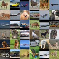
(a)

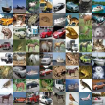
(b)

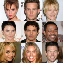
(c)

Figure 1: Qualitative results of RDGAN on 2 datasets STL-10, CIFAR-10 and CelebA-HQ.

Model	FID$\downarrow$	Recall$\uparrow$
Our	13.07	0.47
DDGAN [51]	21.79	0.40
StyleFormer [34]	15.17	-
TransGAN [16]	18.28	-
SNGAN [31]	40.1	-
StyleGAN2+ADA [18]	13.72	0.36

Table 3: Quantitative performance of RDGAN on STL-10.
RDGAN surpasses DDGAN at both metric FID and Recall.

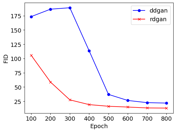
Table 4: The training convergence on STL-10 between DDGAN and RDGAN.

4.2 Robustness Generation

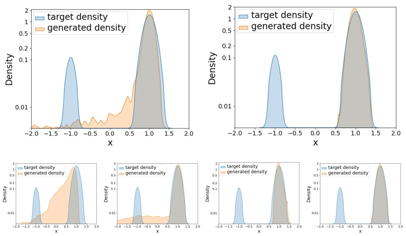
Figure 2: Outlier Robustness on Toy Dataset with $5\%$ outliers. The toy dataset is a mixture of two gaussians $\mathcal{N}(1,0.1)$ (clean dataset), $\mathcal{N}(-1,0.05)$ (outlier dataset) with the mixture rate is ($0.95,0.05$). In the first row, subplots compare target and generated densities between DDGAN and RDGAN. Left: DDGAN; Right: RDGAN. The second row showcases partial timestep RDGAN results. From left to right, semi-dual UOT loss is applied to the first 1, 2, 3 timesteps, and then to all timesteps.

To demonstrate the effectiveness of our RDGAN method on noisy datasets, we initially compare the generated density obtained by training RDGAN and DDGAN techniques with the ground truth target density on a toy dataset. As illustrated in Fig. 2, we visually observe that RDGAN exclusively generates new data points that align with the clean mode on the right, whereas DDGAN produces outlier data scattered between the two modes. This experiment highlights the vulnerability of DDGAN to outliers and underscores the superior reliability of our RDGAN method in noisy training datasets.

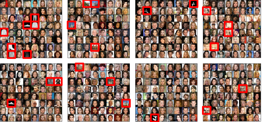
Figure 3: From left to right is corresponding to CE+FT, CE+CH, CE+MT and CE+FCE dataset. Top: DDGAN, Bottom: RDGAN. For the dataset CI+MT, please refer to the second column Figure Fig. 4. The red boxes indicate the synthesized outliers among the clean synthesized samples.

Furthermore, we conducted experiments with RDGAN on various high-dimensional datasets perturbed with diverse noise types, mirroring real-world applications to validate its robustness in handling noisy datasets. As shown in Tab. 8, we trained both RDGAN and DDGAN in scenarios where there is a $5\%$ outlier presence in noisy datasets. Since the resolution of clean and outlier datasets might be different, we rescaled the clean and outlier datasets to the same resolution, with CI+MI at $32\times 32$ resolution and the other four datasets (CE+FT, CE+MT, CE+CH and CE+FCE) at $64\times 64$. Here, CI, MI, FT, CE, CH and FCE stand for CIFAR10, MNIST, FASHION MNIST, CELEBAHQ, LSUN CHURCH and VERTICAL FLIP CELEBAHQ, respectively; and CI+MI means that CIFAR10 peturbed with $5\%$ MNIST. The results in Tab. 8 demonstrate that RDGAN significantly outperforms DDGAN across all noisy datasets. For instance, on the CI+MT dataset, RDGAN surpasses DDGAN by more than 4 points in the FID score. Our technique also proves effective with various outlier datasets, as evidenced by CE+FT, CE+MT, CE+CH and CE+FCE, where we keep the same clean dataset and change the outlier dataset. We observe that RDGAN performs well with both outlier dataset FT and MT which are grayscale and visually different from CE, with an FID gap of around 3 points when compared with the corresponding DDGAN model. Notably, even though the CH dataset comprises RGB images and bears great similarity to CE, RDGAN effectively learns to automatically eliminate outliers, achieving a 2-point lower FID than DDGAN. For hard outlier dataset FCE, which have a great similarity with CE and is practical in the real world, RDGAN successful remove the vertical flip face (refer to last column of Fig. 3) and we achieve better FID score comparing to DDGAN. This demonstrates RDGAN’s capability to discriminate between two datasets in the same RGB domain, which has not previously been reported by other robust generative works [3, 25, 6]. For the qualitative result of the experiment in Tab. 8, refer to the Fig. 3. Our method also outperforms existing robustness methods, which also deal with noisy datasets, as shown in Tab. 5. RDGAN, with FID of 4.82, outperforms the second-best method (UOTM) by nearly 3 points.

When dealing with a perturbed dataset, the simple traditional approach is to preprocess it to remove the outliers. The approach can be used in parallel with RDGAN for better outlier robustness. As presented in Sec. 4, RDGAN can even outperform DDGAN in clean datasets (Tab. 1,Tab. 2, Tab. 4). Therefore, even if we can remove all outliers, using RDGAN instead of DDGAN can provide better performance. For the dataset of CELEBAHQ $64\times 64$ perturbed by $5\%$ of Fashion-MNIST images, we apply isolation forest [27] for preprocessing, which raises the clean ratio to $97\%$. We then train DDGAN on the preprocessed data and achieve the FID of $11.3$, which is significantly worse than RDGAN trained on raw data with FID of 7.89.

4.3 Ablation Studies

4.3.1 Choice of $\Psi_{1}^{*}$ and $\Psi_{2}^{*}$

Given that we could choose $\mathsf{D}_{\Psi_{i}}$ as Csiszár-divergences, commonly used functions like KL and $\chi^{2}$ were tested as choices for $\Psi_{1}$ and $\Psi_{2}$ in RDGAN. However, using KL as ${\Psi_{i}}$ led to infinite loss during RDGAN training, even with meticulous hyperparameter tuning, likely due to the exponential convex conjugate form of KL (refer to Appendix B). For $\chi^{2}$ as ${\Psi_{i}}$, the first row of Tab. 6 reveals that RDGAN with $\chi^{2}$ achieved an FID score of $5.04$, outperforming DDGAN’s FID of $8.81$ on CIFAR-10 with $5\%$ outlier MNIST. While RDGAN with $\chi^{2}$ excels with noisy datasets containing outliers, its performance lags behind DDGAN on clean datasets. Inspired by prior works such as [31, 51], which employ the softplus function instead of other divergences, we conducted RDGAN experiments with ${\Psi_{i}^{*}}=\text{Softplus}$. Interestingly, this function proves highly effective, surpassing both DDGAN and RDGAN with $\chi^{2}$ on both clean and noisy datasets. Since [1] show the Lipschitz loss functions result in better performance, the reason why using softplus as $\Psi_{1}^{*}$ achieve better performance compared to convex conjugate of KL and $\chi^{2}$ could be its Lipschitz continuity property (convex conjugates of KL and $\chi^{2}$ are not Lipschitz). See Appendix B for proof of Lipschitz.

	UOTM [6]	RobustGAN [3]	RDGAN
FID	7.64	15.29	4.82

Table 5: Comparison of RDGAN with other robust generative frameworks (CIFAR-10 perturbed by 5% MNIST)

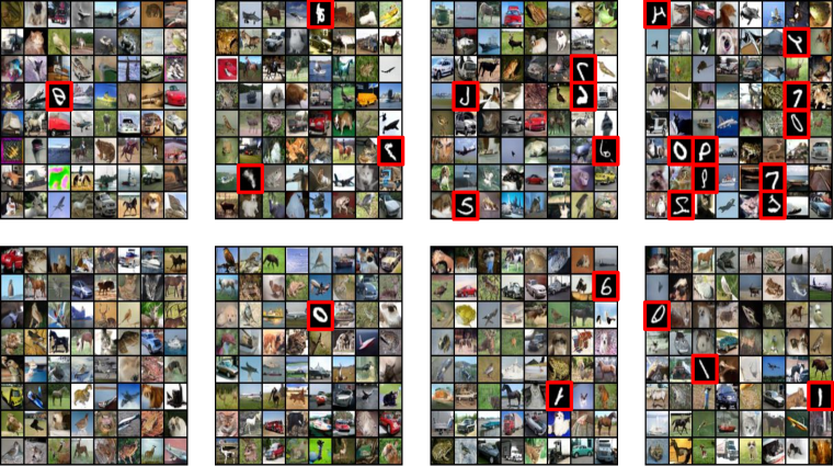
Figure 4: From left to right is corresponding to $3\%,5\%,7\%$ and $10\%$ MNIST outlier in noisy CIFAR-10 dataset. The first row is the DDGAN and the second row is the RDGAN. The red boxes indicate the synthesized outliers among the clean synthesized samples.

4.3.2 Perturbation Ratio

$\Psi_{1}^{*}$	$\Psi_{2}^{*}$	FID (clean) $\downarrow$	FID ($5\%$) $\downarrow$
$\chi^{2}$	$\chi^{2}$	3.93	5.04
softplus	softplus	3.53	4.82
None	None	3.75	8.81

Table 6: The choice of $\Psi_{1}^{*}$ and $\Psi_{2}^{*}$. The FID (clean) and FID ($5\%$) are computed FID on clean CIFAR-10 and CIFAR10 with $5\%$ MNIST outlier. The last row in the table is the DDGAN.

	Synthesized Outlier		FID
Perturbation ratio	DDGAN	RDGAN	DDGAN	RDGAN
$3\%$	$3.2\%$	$0.2\%$	4.76	3.89
$5\%$	$4.1\%$	$1.7\%$	8.81	4.82
$7\%$	$6.9\%$	$2.3\%$	9.55	5.17
$10\%$	$9.8\%$	$3.8\%$	14.77	6.09

Table 7: Synthesized Outlier Ratios and FID Scores of DDGAN and RDGAN trained on datasets with varying perturbation ratios.

	CI+MT	CE+FT	CE+MT	CE+CH	CE+FCE
RDGAN	4.42	7.89	9.29	7.86	5.99
DDGAN	8.81	10.68	12.95	9.83	6.48

Table 8: FIDs comparison between DDGAN and RDGAN on five noisy datasets.

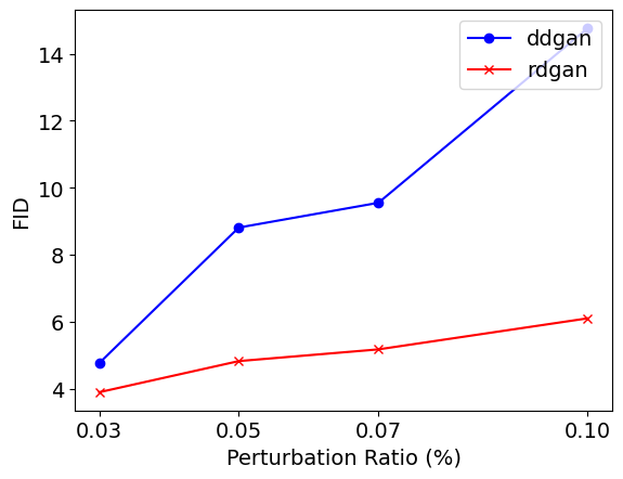
Figure 5: Plot of FIDs comparison between RDGAN and DDGAN on CIFAR-10 data perturbed by MNIST.

As shown in Tab. 8 and Tab. 8, RDGAN consistently maintains strong performance even as the outlier percentage in training datasets (CI + MT) increases. While the perturbation ratio in the training dataset escalates from $3\%$ to $10\%$, RDGAN’s FID only increases by around 2 points (from $3.90$ to $6.09$). In contrast, DDGAN’s FID increases by more than 10 points (from $4.76$ to $14.77$), and the synthesized outlier ratio of RDGAN rises from $0.2\%$ to $3.8\%$ compared to DDGAN’s increase from $3.2\%$ to $9.8\%$.

4.3.3 Partial Timestep RDGAN

As DDGAN comprises multiple diffusion steps that are trained with adversarial networks, and RDGAN introduces the semi-dual UOT loss in place of the traditional GAN loss, a natural question arises: How well does RDGAN perform when only partially applying the proposed loss within the DDGAN framework? Referring to Fig. 2, it becomes evident that the performance of RDGAN with partial timesteps falls behind that of RDGAN with all timesteps, referred to simply as “RDGAN” in other sections of this paper. This discrepancy may be attributed to the fact that RDGAN has demonstrated the ability to either maintain or surpass DDGAN performance on both clean and perturbed images, making full-timestep RDGAN the superior choice over partial-timestep RDGAN.

5 Conclusion

In this paper, we have highlighted the limitations of the DDGAN model when faced with noisy datasets containing outliers. To address this issue, we have introduced the RDGAN technique, which incorporates Semi-Dual UOT into the DDGAN framework. RDGAN has demonstrated the ability to either maintain or enhance performance across all three critical generative modeling criteria: mode coverage, high-fidelity generation, and fast sampling, all while ensuring rapid training convergence. Additionally, our paper showcases that RDGAN significantly outperforms DDGAN on noisy training datasets with various settings, making it a promising approach for real-world noisy datasets. Moreover, our work is complementary to other DDGAN improvement techniques, such as WaveDiff [35], suggesting potential to raise robustness of those models in the future.

Supplementary Material

6 Detailed Experiments

6.1 Network configurations

6.1.1 Generator.

Our generator follows a UNet-like architecture primarily inspired by NCSN++ [45, 51]. Detailed configurations of the generator for each dataset can be found in Tab. 9.

6.1.2 Discriminator.

The discriminator has the same number of layers as the generator. Further details about the discriminator’s structure can be found in [51].

	CIFAR-10	STL-10	CELEBAHQ	CI+MT	CE+{CH,FT,MT}	CE+FCE
# of ResNet blocks per scale	2	2	2	2	2	2
Base channels	128	128	64	128	96	128
Channel multiplier per scale	(1,2,2,2)	(1,2,2,2)	(1,1,2,2,4,4)	(1,2,2,2)	(1,2,2,2,4)	(1,2,2,2,4)
Attention resolutions	16	16	16	16	16	16
Latent Dimension	100	100	100	100	100	100
# of latent mapping layers	4	4	4	4	4	4
Latent embedding dimension	256	256	256	256	256	256

Table 9: Network configurations.

6.2 Training Hyperparameters

For the sake of reproducibility, we have provided a comprehensive table of tuned hyperparameters in Tab. 10. Our hyperparameters align with the baseline [51], with minor adjustments made only to the number of epochs and the allocation of GPUs for specific datasets. In terms of training times, models for CIFAR-10 and STL-10 take 1.6 and 3.6 days, respectively, on a single GPU. For CI-MT and CE+{CH,FT,MT}, it takes 1.6 and 2 day GPU hours, correspondingly.

	CIFAR-10	STL-10	CELEBAHQ	CI+MT	CE+{CH,FT,MT}	CE+FCE
$\text{lr}_{G}$	$1.6\text{e-4}$	$1.6\text{e-}4$	$1\text{e-}4$	$1.6\text{e-}4$	$1.6\text{e-}4$	$8\text{e-}5$
$\text{lr}_{D}$	$1.25\text{e-}4$	$1.25\text{e-}4$	$2\text{e-}4$	$1.25\text{e-}4$	$1.\text{e-}4$	$5\text{e-}5$
Adam optimizer ($\beta_{1}$ & $\beta_{2}$)	0.5, 0.9	0.5, 0.9	0.5, 0.9	0.5, 0.9	0.5, 0.9	0.5, 0.9
EMA	0.9999	0.9999	0.9999	0.999	0.999	0.9999
Batch size	256	72	256	48	72	96
Lazy regularization	15	15	10	15	15	15
# of epochs	1800	1200	800	1800	800	800
# of timesteps	4	4	2	4	2	2
# of GPUs	1	1	2	2	1	2
r1 gamma	0.02	0.02	2.0	0.02	0.02	2
Tau $\tau$ (only for RDGAN)	1e-3	1e-4	1e-7	1e-3	3e-4	1e-3

Table 10: Choices of hyper-parameters

6.3 Dataset Preparation

Clean Dataset: We conducted experiments on two clean datasets CIFAR-10 ($32\times 32$) and STL-10 ($64\times 64$). For training, we use 50,000 images.

Noisy Dataset:

• CI+MI: We resize the MNIST data to resolution of ($32\times 32$) and mix into CIFAR-10. The total samples of this dataset is 50,000 images.

• CE+{CH,FT,MT,FCE}: We resize the CelebHQ and CIFAR-10, FASHION MNIST, LSUN CHURCH to the resolution of ($64\times 64$), flip CelebHQ vertically, and mix them together. The CelebHQ is clean, and the others are outlier datasets. The noisy datasets contain 27,000 training images.

6.4 Evaluation Protocol

We measure image fidelity by Frechet inception distance (FID) [13] and measure sample diversity by Recall metric [23].

FID: We compute FID between ground truth clean dataset and 50,000 generated images from the models

Recall: Similar to FID, we compute Recall between ground truth dataset and 50,000 generated images from the models

Outlier Ratio: We train classifier models between clean and noisy datasets and use them to classify the synthesized outliers. We first generate 50,0000 synthesized images and count all the outliers from them.

7 Criteria for choosing $\Psi$

To choose $\Psi_{1}$ and $\Psi_{2}$ for this loss function, we recommend two following criteria. First, $\Psi_{1}$ and $\Psi_{2}$ could make the trade-off between the transport map $\pi$ in Eq. 7 and the hard constraint on the marginal distribution $\mu$ to $\nu$ in order to seek another relaxed plan that transports masses between their approximation but may sharply lower the transport cost. From the view of robustness, this relaxed plan can ignore some masses from the source distribution of which the transport cost is too high, which can be seen as outliers. Second, $\Psi_{1}$ and $\Psi_{2}$ need to be convex and differentiable so that Eq. 9 holds.

Two commonly used candidates for $\Psi_{1}$ and $\Psi_{2}$ are two f-divergence KL ($f(x)=x\ln x$ if $x>0$ else $f(x)=\infty$) and $\chi^{2}$ ($f(x)=(x-1)^{2}$ if $x>0$ else $f(x)=\infty$). However, the convex conjugate of KL is an exponential function, making the training process for DDGAN complicated due to the dynamic of loss value between its many denoising diffusion time steps. Among the ways we tune the model, the loss functions of both generator and discriminator models keep reaching infinity.

Thus, we want a more ”stable” convex conjugate function. That of $\chi^{2}$ is quadratic polynomial, which does not explode when $x$ increases like that of KL:

$$\Psi^{*}(x)=\begin{cases}\frac{1}{4}x^{2}+x,&\text{ if }x\geq-2\\ -1,&\text{ if }x<-2\end{cases}$$ (15)

However, it is still not Lipschitz continue.

As stated in section Sec. 3, we hypothesize that Lipschitz continuity of Softplus can raise the training effectiveness while convex conjugate of KL and $\chi^{2}$ are not Lipschitz. Here, we provide the proofs of Lipschitz. But first, we reiterate that the convex conjugate of a function $f:\mathbb{R}\rightarrow(-\infty,\infty)$ is defined as:

$$f^{*}(x)=\sup_{y\in\mathbb{R}}\{\langle x,y\rangle-f(y)\}$$ (16)

a) Convex conjugate of KL function is non-Lipschitz

Let $\Psi(y)=y\ln y$ if $y>0$ else $\Psi(y)=\infty$

$$\Psi^{*}(x)=e^{x-1}$$ (17)

Choose $x_{1}=a+1$ and $x_{2}=a+1+\epsilon$, $\epsilon>0$. We have:

$$\frac{|\Psi^{*}(x_{1})-\Psi^{*}(x_{2})|}{|x_{2}-x_{1}|} =\frac{|e^{a+\epsilon}-e^{a}|}{\epsilon}$$ (18)

$$=e^{a}\frac{|e^{\epsilon}-1|}{\epsilon}$$ (19)

$$\overset{a\to\infty}{\longrightarrow}\infty$$ (20)

Thus, $\frac{|\Psi^{*}(x_{2})-\Psi^{*}(x_{2})|}{|x_{2}-x_{1}|}$ does not have an upper bound, and convex conjugate of KL function is non-Lipschitz.

b) Convex conjugate of $\chi^{2}$ function is non-Lipschitz

Convex conjugate of $\chi^{2}$ function $\Psi*$ is defined as Eq. 15.

Choose $x_{1}=a$ and $x_{2}=a+\epsilon$, $a>0$, $\epsilon>0$. We have:

$$\frac{|\Psi^{*}(x_{2})-\Psi^{*}(x_{2})|}{|x_{2}-x_{1}|} =\frac{|0.5a\epsilon+0.25\epsilon^{2}+\epsilon|}{\epsilon}$$ (21)

$$=|0.5a+0.25\epsilon+1|$$ (22)

$$\overset{a\to\infty}{\longrightarrow}\infty$$ (23)

Thus, $\frac{|\Psi^{*}(x_{2})-\Psi^{*}(x_{2})|}{|x_{2}-x_{1}|}$ does not have an upper bound, and convex conjugate of KL function is non-Lipschitz.

c) Softplus has Lipschitz continuity property

Let $\Psi^{*}(x)=\ln(1+e^{x})$, $a>0$. We have:

$$|\Psi^{*}(x+a)-\Psi^{*}(x)| =|\ln(1+e^{x+a})-\ln(1+e^{x})|$$ (24)

$$=|\ln(\frac{1+e^{x+a}}{1+e^{x}})|$$ (25)

$$\leq|\ln(\frac{e^{a}+e^{x+a}}{1+e^{x}})|$$ (26)

$$=|\ln(e^{a})|$$ (27)

$$=a$$ (28)

$$<2a$$ (29)

$$=2|(x+a)-x|$$ (30)

Remark: For any function $f$, its convex conjugate is always semi-continuous, and $f=f^{**}$ if and only if $f$ is convex and lower semi-continuous [24]. So, we can choose $f^{*}$ first such that this is a non-decreasing, differentiable, and semi-continuous function. Then, we find $f^{**}$ and check if $f^{***}$ and $f^{*}$ is equal. If $f^{***}$ and $f^{*}$, $f^{**}$ will be a function of which convex conjugate is $f^{*}$. Then we will check if $f^{**}$ satisfied the first criterion to use it as $\Psi_{1}$ or $\Psi_{2}$.

With this remark, we can see why functions whose convex conjugate is a simple linear function cannot filter out outliers.

If $\Psi^{*}(x)=ax+b$, $(a>0)$, we have:

$$\Psi(x)=\begin{cases}a,&\text{ if }x=a\\ \infty,&\text{ if }x\neq a\end{cases}$$ (31)

As a result, with equation Eq. 7, the UOTM cost is finite only when $\frac{d\pi_{1}}{d\mu}=\frac{d\pi_{2}}{d\nu}=a$ (constant). We will prove the unbalanced optimal transport map is the same as the optimal transport map of the origin OT problem scaled by $a$.

Let $\pi^{*}$ be the optimal transport map of the OT problem Eq. 32. Then, the marginal distribution of $\pi^{*}$ is $\mu$ and $\nu$. Recall that

$$\mathsf{OT}(\mu,\nu)=\min_{\pi\in\Pi(\mu,\nu)}\int c(x,y)d\pi(x,y),$$ (32)

$$\mathsf{UOT}(\mu,\nu) =\min_{\pi\in{\mathcal{M}}({\mathcal{X}}\times{\mathcal{X}})}\int c(x,y)d\pi(x,y)$$

$$+\mathsf{D}_{\Psi}(\pi_{1}\|\mu)+\mathsf{D}_{\Psi}(\pi_{2}\|\nu),$$ (33)

In the UOT problem Eq. 33, the transport cost is finite only when the transport map $\bar{\pi}$ has the marginal distribution $\bar{\pi}_{1}=a\mu$ and $\bar{\pi}_{2}=a\nu$, which satisfies $\frac{d\bar{\pi}_{1}}{d\mu}=\frac{d\bar{\pi}_{2}}{d\nu}=a$. Thus, $\mathsf{D}_{\Psi}(\pi_{1}\|\mu)+\mathsf{D}_{\Psi}(\pi_{2}\|\nu)=C$ is a constant.

As a result, finding the optimal unbalanced transport map for Eq. 33 is equivalent to find

$$\operatorname*{arg\,min}_{\pi\in\Pi(a\mu,a\nu)}\int c(x,y)d\pi(x,y)$$

We also have

$$\min_{\pi\in\Pi(a\mu,a\nu)}\int c(x,y)d\pi(x,y)=\mathsf{OT}(a\mu,a\nu)=a\mathsf{OT}(\mu,\nu)$$

Let $\bar{\pi}^{*}=a\pi^{*}$, we have:

$$\int c(x,y)d\bar{\pi}^{*}(x,y)=a\int c(x,y)d\pi^{*}(x,y)=a\mathsf{OT}(\mu,\nu)$$

Therefore, $a\pi^{*}$ is the optimal transport map of the UOT problem (Q.E.D). Lastly, we will explain intuitively why using Softplus can filter out abnormal data.

First, using the Remark in this section, given $\Psi^{*}(x)=\ln(1+e^{x})$, we have:

$$\Psi=\begin{cases}x\ln x+(1-x)\ln(1-x),&\text{if }x\in(0;1)\\ \infty,&\text{otherwise}\end{cases}$$ (34)

Compared to the penalized linear function (refer to Eq. 31), the UOT problem with the convex conjugate function of Softplus does not reduce to a normal OT problem.

Assume that $\mathsf{D}_{\Psi}(\pi_{1}\|\mu)+\mathsf{D}_{\Psi}(\pi_{2}\|\nu)$ attains its minimum at $\zeta$ (Eq. 33), then if $\frac{d\pi_{1}}{d\mu}=\frac{d\pi_{2}}{d\nu}=\zeta$, then it reduces the UOT problem to an OT problem.

However, if there are outliers, which means that the transportation costs at some locations are very large, then one can decrease mass at those locations of $\pi$ so that the change of $\mathsf{D}_{\Psi}(\pi_{1}\|\mu)+\mathsf{D}_{\Psi}(\pi_{2}\|\nu)$ is much smaller than the decrease in total transportation cost $\int c(x,y)d\pi(x,y)$. It explains why both KL and Softplus have the ability to filter out outliers.

It is noteworthy that, despite sharing many similarities, the convex conjugate functions of these two functions are very different, with Softplus owing some benefits due to its Lipschitz continuity property.

(a)

(b)

Figure 6: The graph of KL function and function whose convex conjugate is Softplus.

8 Additional Results

As discussed in Sec. 4, RDGAN converges faster than DDGAN. As can be seen clearly in Fig. 7, at epoch 300, the generated images of RDGAN have much higher qualities compared to those of DDGAN. We show the non-curated qualitative figure of RDGAN on clean datasets in Fig. 8, Fig. 9, Fig. 10.

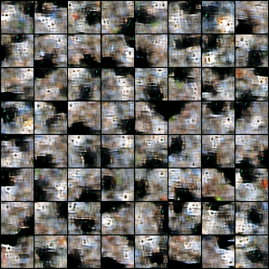
(a)

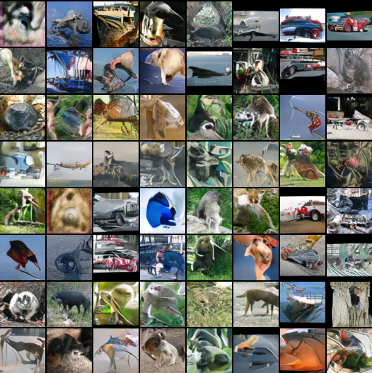
(b)

Figure 7: Qualitative comparison of RDGAN and DDGAN on STL-10 at epoch 300. RDGAN converges faster than DDGAN.

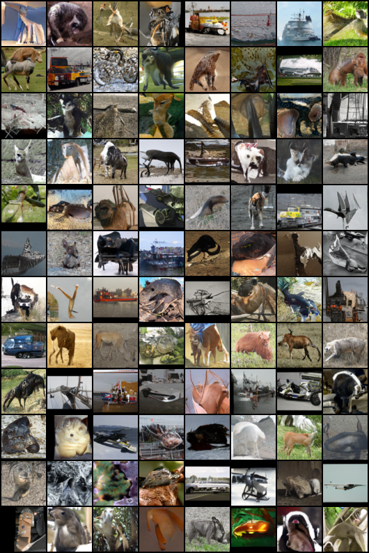
Figure 8: Non-curated STL-10 qualitative images.

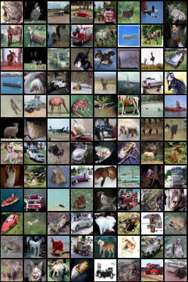
Figure 9: Non-curated CIFAR-10 qualitative images.

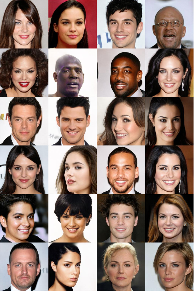
Figure 10: Non-curated CELEBAHQ-256 qualitative images.

References

- Akbari et al. [2021] Ali Akbari, Muhammad Awais, Manijeh Bashar, and Josef Kittler. How does loss function affect generalization performance of deep learning? application to human age estimation. In International Conference on Machine Learning, pages 141–151. PMLR, 2021.
- Arjovsky et al. [2017] Martin Arjovsky, Soumith Chintala, and Léon Bottou. Wasserstein generative adversarial networks. In International conference on machine learning, pages 214–223. PMLR, 2017.
- Balaji et al. [2020] Y. Balaji, R. Chellappa, and S. Feizi. Robust optimal transport with applications in generative modeling and domain adaptation. In NeurIPS, 2020.
- Chizat et al. [2018a] Lenaic Chizat, Gabriel Peyré, Bernhard Schmitzer, and François-Xavier Vialard. Scaling algorithms for unbalanced optimal transport problems. Mathematics of Computation, 87(314):2563–2609, 2018a.
- Chizat et al. [2018b] Lenaic Chizat, Gabriel Peyré, Bernhard Schmitzer, and François-Xavier Vialard. Unbalanced optimal transport: Dynamic and kantorovich formulations. Journal of Functional Analysis, 274(11):3090–3123, 2018b.
- Choi et al. [2023] Jaemoo Choi, Jaewoong Choi, and Myungjoo Kang. Generative modeling through the semi-dual formulation of unbalanced optimal transport. arXiv preprint arXiv:2305.14777, 2023.
- Coates et al. [2011] Adam Coates, Andrew Ng, and Honglak Lee. An analysis of single-layer networks in unsupervised feature learning. In Proceedings of the Fourteenth International Conference on Artificial Intelligence and Statistics, pages 215–223, Fort Lauderdale, FL, USA, 2011. PMLR.
- Dao et al. [2023] Quan Dao, Hao Phung, Binh Nguyen, and Anh Tran. Flow matching in latent space. arXiv preprint arXiv:2307.08698, 2023.
- Dhariwal and Nichol [2021] Prafulla Dhariwal and Alexander Nichol. Diffusion models beat gans on image synthesis. Advances in Neural Information Processing Systems, 34:8780–8794, 2021.
- Esser et al. [2020] Patrick Esser, Robin Rombach, and Björn Ommer. Taming transformers for high-resolution image synthesis, 2020.
- Gallouët et al. [2021] Thomas Gallouët, Roberta Ghezzi, and François-Xavier Vialard. Regularity theory and geometry of unbalanced optimal transport. arXiv preprint arXiv:2112.11056, 2021.
- Gulrajani et al. [2017] Ishaan Gulrajani, Faruk Ahmed, Martin Arjovsky, Vincent Dumoulin, and Aaron C Courville. Improved training of wasserstein gans. Advances in neural information processing systems, 30, 2017.
- Heusel et al. [2017] Martin Heusel, Hubert Ramsauer, Thomas Unterthiner, Bernhard Nessler, and Sepp Hochreiter. Gans trained by a two time-scale update rule converge to a local nash equilibrium. Advances in neural information processing systems, 30, 2017.
- Ho et al. [2020] Jonathan Ho, Ajay Jain, and Pieter Abbeel. Denoising diffusion probabilistic models. In Advances in neural information processing systems, 2020.
- Huang et al. [2021] Chin-Wei Huang, Jae Hyun Lim, and Aaron C Courville. A variational perspective on diffusion-based generative models and score matching. Advances in Neural Information Processing Systems, 34:22863–22876, 2021.
- Jiang et al. [2021] Yifan Jiang, Shiyu Chang, and Zhangyang Wang. Transgan: Two pure transformers can make one strong gan, and that can scale up. Advances in Neural Information Processing Systems, 34:14745–14758, 2021.
- Karras et al. [2018] Tero Karras, Timo Aila, Samuli Laine, and Jaakko Lehtinen. Progressive growing of GANs for improved quality, stability, and variation. In International Conference on Learning Representations, 2018.
- Karras et al. [2020a] Tero Karras, Miika Aittala, Janne Hellsten, Samuli Laine, Jaakko Lehtinen, and Timo Aila. Training generative adversarial networks with limited data. In Advances in neural information processing systems, 2020a.
- Karras et al. [2020b] Tero Karras, Samuli Laine, Miika Aittala, Janne Hellsten, Jaakko Lehtinen, and Timo Aila. Analyzing and improving the image quality of stylegan. In Proceedings of the IEEE conference on computer vision and pattern recognition, 2020b.
- K.Fatras et al. [2021] K.Fatras, T.Séjourne, N.Courty, and R.Flamary. Unbalanced optimal transport; applications to domain adaptation. International conference of Machine Learning, 2021.
- Kingma et al. [2021] Diederik Kingma, Tim Salimans, Ben Poole, and Jonathan Ho. Variational diffusion models. Advances in neural information processing systems, 34:21696–21707, 2021.
- Krizhevsky [2012] Alex Krizhevsky. Learning multiple layers of features from tiny images. University of Toronto, 2012.
- Kynkäänniemi et al. [2019] Tuomas Kynkäänniemi, Tero Karras, Samuli Laine, Jaakko Lehtinen, and Timo Aila. Improved precision and recall metric for assessing generative models. Advances in Neural Information Processing Systems, 32, 2019.
- Lai and Lin [1988] Hang-Chin Lai and Lai-Jui Lin. The fenchel-moreau theorem for set functions. Proceedings of the American Mathematical Society, 103(1):85–90, 1988.
- Le et al. [2021] K. Le, H. Nguyen, Q. Nguyen, N. Ho, T. Pham, and H. Bui. On robust optimal transport: Computational complexity and barycenter computation. 2021.
- Le et al. [2023] Thanh Le, Hao Phung, Thuan Nguyen, Quan Dao, Ngoc Tran, and Anh Tran. Anti-dreambooth: Protecting users from personalized text-to-image synthesis. In Proceedings of the IEEE/CVF International Conference on Computer Vision (ICCV), 2023.
- Liu et al. [2008] Fei Tony Liu, Kai Ming Ting, and Zhi-Hua Zhou. Isolation forest. In 2008 eighth ieee international conference on data mining, pages 413–422. IEEE, 2008.
- Lou and Ermon [2023] Aaron Lou and Stefano Ermon. Reflected diffusion models. arXiv preprint arXiv:2304.04740, 2023.
- Lu et al. [2022] Cheng Lu, Yuhao Zhou, Fan Bao, Jianfei Chen, Chongxuan Li, and Jun Zhu. Dpm-solver: A fast ode solver for diffusion probabilistic model sampling in around 10 steps. arXiv preprint arXiv:2206.00927, 2022.
- Meng et al. [2021] Chenlin Meng, Yutong He, Yang Song, Jiaming Song, Jiajun Wu, Jun-Yan Zhu, and Stefano Ermon. Sdedit: Guided image synthesis and editing with stochastic differential equations. arXiv preprint arXiv:2108.01073, 2021.
- Miyato et al. [2018] Takeru Miyato, Toshiki Kataoka, Masanori Koyama, and Yuichi Yoshida. Spectral normalization for generative adversarial networks. arXiv preprint arXiv:1802.05957, 2018.
- Nguyen et al. [2022] K. Nguyen, D. Nguyen, Q.Nguyen, T.Pham, H.Bui, D.Phung, T.Le, and N.Ho. On transportation of mini-batches: A hierarchical approach. International Conference of Machine Learning, 2022.
- Nietert et al. [2022] Sloan Nietert, Ziv Goldfeld, and Rachel Cummings. Outlier-robust optimal transport: Duality, structure, and statistical analysis. In International Conference on Artificial Intelligence and Statistics, pages 11691–11719. PMLR, 2022.
- Park and Kim [2021] Jeeseung Park and Younggeun Kim. Styleformer: Transformer based generative adversarial networks with style vector, 2021.
- Phung et al. [2023] Hao Phung, Quan Dao, and Anh Tran. Wavelet diffusion models are fast and scalable image generators. In Proceedings of the IEEE/CVF Conference on Computer Vision and Pattern Recognition (CVPR), pages 10199–10208, 2023.
- Ramesh et al. [2022] Aditya Ramesh, Prafulla Dhariwal, Alex Nichol, Casey Chu, and Mark Chen. Hierarchical text-conditional image generation with clip latents. arXiv preprint arXiv:2204.06125, 2022.
- Rombach et al. [2022] Robin Rombach, Andreas Blattmann, Dominik Lorenz, Patrick Esser, and Björn Ommer. High-resolution image synthesis with latent diffusion models. In Proceedings of the IEEE/CVF Conference on Computer Vision and Pattern Recognition, pages 10684–10695, 2022.
- Rout et al. [2021] Litu Rout, Alexander Korotin, and Evgeny Burnaev. Generative modeling with optimal transport maps. arXiv preprint arXiv:2110.02999, 2021.
- Ruiz et al. [2022] Nataniel Ruiz, Yuanzhen Li, Varun Jampani, Yael Pritch, Michael Rubinstein, and Kfir Aberman. Dreambooth: Fine tuning text-to-image diffusion models for subject-driven generation. 2022.
- Saharia et al. [2022] Chitwan Saharia, William Chan, Saurabh Saxena, Lala Li, Jay Whang, Emily Denton, Seyed Kamyar Seyed Ghasemipour, Burcu Karagol Ayan, S Sara Mahdavi, Rapha Gontijo Lopes, et al. Photorealistic text-to-image diffusion models with deep language understanding. arXiv preprint arXiv:2205.11487, 2022.
- Sanjabi et al. [2018] Maziar Sanjabi, Jimmy Ba, Meisam Razaviyayn, and Jason D Lee. On the convergence and robustness of training gans with regularized optimal transport. Advances in Neural Information Processing Systems, 31, 2018.
- Schiebinger et al. [2019] G. Schiebinger et al. Optimal-transport analysis of single-cell gene expression identifies developmental trajectories in reprogramming. Cell, 176:928–943, 2019.
- Song et al. [2021a] Jiaming Song, Chenlin Meng, and Stefano Ermon. Denoising diffusion implicit models. In International Conference on Learning Representations, 2021a.
- Song et al. [2021b] Yang Song, Conor Durkan, Iain Murray, and Stefano Ermon. Maximum likelihood training of score-based diffusion models. Advances in Neural Information Processing Systems, 34:1415–1428, 2021b.
- Song et al. [2021c] Yang Song, Jascha Sohl-Dickstein, Diederik P Kingma, Abhishek Kumar, Stefano Ermon, and Ben Poole. Score-based generative modeling through stochastic differential equations. In International Conference on Learning Representations, 2021c.
- Vacher and Vialard [2022] Adrien Vacher and François-Xavier Vialard. Stability and upper bounds for statistical estimation of unbalanced transport potentials. arXiv preprint arXiv:2203.09143, 2022.
- Vahdat and Kautz [2020] Arash Vahdat and Jan Kautz. NVAE: A deep hierarchical variational autoencoder. In Advances in neural information processing systems, 2020.
- Villani [2008] Cédric Villani. Optimal transport: Old and new. 2008.
- Wang et al. [2022] Weilun Wang, Jianmin Bao, Wengang Zhou, Dongdong Chen, Dong Chen, Lu Yuan, and Houqiang Li. Semantic image synthesis via diffusion models. arXiv preprint arXiv:2207.00050, 2022.
- Xiao et al. [2021] Zhisheng Xiao, Karsten Kreis, Jan Kautz, and Arash Vahdat. Vaebm: A symbiosis between variational autoencoders and energy-based models. In International Conference on Learning Representations, 2021.
- Xiao et al. [2022] Zhisheng Xiao, Karsten Kreis, and Arash Vahdat. Tackling the generative learning trilemma with denoising diffusion GANs. In International Conference on Learning Representations (ICLR), 2022.
- Zhang and Chen [2022] Qinsheng Zhang and Yongxin Chen. Fast sampling of diffusion models with exponential integrator. arXiv preprint arXiv:2204.13902, 2022.