DyRA: Dynamic Resolution Adjustment For Scale-robust Object Detection

Abstract

In object detection, achieving constant accuracy is challenging due to the variability of object sizes. One possible solution to this problem is to optimize the input resolution, known as a multi-resolution strategy. Previous approaches for optimizing resolution are often based on pre-defined resolutions or a dynamic neural network, but there is a lack of study for run-time resolution optimization for existing architecture. In this paper, we propose an adaptive resolution scaling network called DyRA, which comprises convolutions and transformer encoder blocks, for existing detectors. Our DyRA returns a scale factor from an input image, which enables instance-specific scaling. This network is jointly trained with detectors with specially designed loss functions, namely ParetoScaleLoss and BalanceLoss. The ParetoScaleLoss produces an adaptive scale factor from the image, while the BalanceLoss optimizes the scale factor according to localization power for the dataset. The loss function is designed to minimize accuracy drop about the contrasting objective of small and large objects. Our experiments on COCO, RetinaNet, Faster-RCNN, FCOS, and Mask-RCNN achieved 1.3%, 1.1%, 1.3%, and 0.8% accuracy improvement than a multi-resolution baseline with solely resolution adjustment. The code is available at https://github.com/DaEunFullGrace/DyRA.git.

1 Introduction

Deep learning demonstrated remarkable performance in computer vision applications such as object detection [45, 35] and segmentation [32, 1]. However, achieving consistent accuracy in real-world applications remains a challenge due to the variability of object sizes [44, 6, 23]. The size variation is often significant in object detection, causing diverse accuracy variation [37]. Several solutions have been proposed to deal with this problem, either by optimizing the architecture of the neural networks [25, 28, 23] or augmenting the data [29, 38, 37]. In data augmentation, resolution adjustment can address the problem without changing the network architecture, by taking advantage of varying the resolution of the input images.

Fig. 1 illustrates why varying the image resolution can help to increase detection accuracy. Objects, which have extreme sizes, cannot be detected due to the scale-variant performance of the detector. In such cases, the images containing huge (or tiny) objects can be better processed by scaling them down (or up) to lower (or higher) while matching the resolution to the detector’s ability. If the resolution of the input image can be determined correctly, the detection accuracy will be improved, which is the main focus of this work.

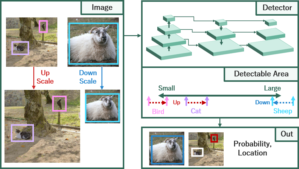
Figure 1: Motivation of judicious image scaling. One way to increase the detection of extreme scales in the dataset is to scale the resolution to match the network’s capacity.

As the resolution is a crucial hyper-parameter for the detection ability [40], careful resolution selection can enable the network to extract richer information, leading to increased accuracy. There are several approaches to optimizing the resolution, which can be categorized into three. The first approach is to scale the input images with predefined resolutions and apply them as data-augmentation to networks [29, 37], which is also applicable to transformer-based networks [41, 30, 31, 49]. The dynamic resolution network [54] enables adaptive resolution by selecting one of these sizes. However, an obvious drawback of this approach is that it requires manual work to determine candidate resolutions, which relies on expert knowledge with lots of trial and error. To eliminate the need for human expertise, the second approach, automated augmentation search [6], enables an optimized resolution for each image/box in the training dataset. The last approach is the run-time adaptive scaling [18] that optimizes the resolution on the fly without any domain-specific expertise.

In this paper, we propose a run-time adaptive scaling network, called DyRA, which produces an image-specific scale factor. DyRA is designed as a separate companion neural network with convolution and transformer encoder blocks, and it is jointly trained with existing object detectors. Fig. 2 illustrates how the proposed image scaler, i.e., DyRA, can be plugged into the detector. Note that the input to the scaler module is an image, while its output is a single scale factor for the resolution. To determine the appropriate scale factor, we introduced additional loss terms to consider for input data and network. An image usually contains many different objects to be detected, which makes it hard to decide the scale factor to provide accuracy gain for all objects. Thus, we defined the loss function to decide the proper scale factor by the single object size and extended it for multiple objects with Pareto optimality [7] and maximum likelihood estimation (MLE) [33]. This loss is called ParetoScaleLoss, which can minimize the accuracy drop of scaling for various scale variations. As the scale factor is determined by box sizes, we modify the scale factor based on the box size range. For an accurate scale factor for the dataset, we optimized the size range based on the detector’s localization power of the training dataset by BalacneLoss.

Different from previous methods, DyRA does not require domain-specific knowledge about the input data. It is also worthwhile to mention that our method is designed to be portable to existing detectors. The automatic scaling decision in Hao et al. [18], for instance, cannot be applied to other object detectors as the entire neural network is customized for the resized image. Our method does not require any architectural modification to the object detector only modifying the inputs. To the best of our knowledge, our network is the first attempt to dynamically optimize the hyper-parameter in a fully separable network from the existing networks. Moreover, our network yields a continuous scale factor that provides extensive scale coverage for higher detection performance. This is important because the resolution has a continuous domain, but selecting from a few discrete sizes can lead to a distribution mismatch.

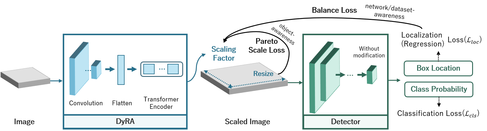
Figure 2: Overview of DyRA. The architecture for detecting objects consists of 2-networks: the DyRA and the original detector. First, the DyRA aims to estimate the scale factor from the given image to scale it. After resizing the image by a scale factor, the detector classifies and localizes objects from the resized image as a general inference process. The network is optimized by two additional loss functions for data-adaptiveness, which are ParetoScaleLoss and BalacneLoss.

We verified the effectiveness of the proposed approach with various object detectors on MS-COCO [24] and PascalVOC [13]. For the anchor-based detector, we achieved improvements in accuracy (average precision, AP) by 1.3% on RetinaNet [26], by 1.0% on Faster R-CNN [36] and by 0.8% on Mask-RCNN compared to the multi-resolution strategy in COCO2017. In anchor-free detector, DyRA provides accuracy improvement by 1.3% for FCOS [42].

2 Related Work

Object Detection Networks. Object detection is an application that identifies and localizes objects from images. The majority of object detectors typically comprise three components, namely the backbone, neck, and head. The backbone is responsible for extracting characteristics from the image, thus pre-trained image classifiers such as [19, 47, 39] are widely used. Based on the backbone, the neck [25, 28, 53, 15] extracts multi-scale features utilized as in the subsequent detection procedure. The head receives these features as input and finalizes the detection process, including localization and classification. There have been two approaches to the implementation of the head in object detection: one-stage [35, 29, 26, 3, 43] and two-stage [45, 36, 16, 20] networks. One-stage networks can attain low inference latency with unified head architecture, while two-stage networks have relatively high inference latency due to an accurate detection process with an additional refinement network. Anchor-free detectors [42, 50, 48, 12] have been introduced to address hyper-parameters in the head while reducing latency by eliminating the need for the non-maximum suppression (NMS) operation. Since our method is based on input image scaling, it is agnostic to object detection neural network topology.

Image-level Multi-resolution Strategies. As stated earlier, image resolution is an important parameter that affects detection accuracy. Therefore, there have been several previous works that take multiple resolutions into account. Based on how and when resolutions are exploited, we can classify them into the following three categories:

• Predefined multiple resolutions: The simplest way is to apply a set of multiple resolutions as a data augmentation strategy [29, 38, 37]. This approach can be used to improve the scale coverage of any neural network architectures, including transformer-based networks [41, 30, 31, 49]. A recent transformer-based detection, multi-resolution patchification [2] was proposed to minimize information loss for resizing operation with the same objectivity from the multi-resolution approach. The dynamic resolution selection technique proposed by Zhu et al. [54] is also based on the predefined resolutions; it selects one of the predefined resolutions at the classification stage.

• Automated data augmentation: In contrast to the predefined approach, there have been some attempts to automate this data augmentation without human expertise. Cubuk et al. [8, 9] proposed image augmentation techniques that automatically combine color-based and resolution-based augmentations. Based on this, Chen et al. [6] proposed a box-/image-level augmentation to deal with the scale variance.

• Run-time scaling: The last approach is to adaptively adjust the input image at run-time to achieve better scale coverage. Hao et al. [18] took this approach in their face detection application. They determined the appropriate scale factor from the single-scale Region Proposal Network (RPN). It was shown that such dynamic re-scaling can lead to a significant improvement in scale coverage, but it is not directly applicable to other applications because their re-scaling decision is tightly coupled to their internal neural network structure. However, our network is easily integrated into different neural networks.

Dynamic Neural Networks. Dynamic neural networks [17] refer to neural networks with architectures or parameters that can be adaptively reconfigured on the fly. While the vast majority of dynamic neural networks aim to reduce the computational cost, some works try to improve the accuracy of the neural network, similar to our approach. A kernel-wise dynamic sampling [10, 55, 14] in convolutions enables an adaptive receptive field, enhancing representation capabilities. A dynamic activation function [5] can improve representation ability with adaptable piece-wise linear activation. In a more coarse-grained view, feature-level dynamic attentions [21, 22] offer channel-wise attention by weighting on the salient features. For multi-scale architecture, branch-wise soft attention network [44] offers additional information in an image-specific approach. Architectural dynamic neural networks [34, 4, 46, 11] exit the layer after sufficiently accurate results are achieved. In object detection, the dynamic early exit method [52, 27] was adopted by cascading multiple backbone networks.

3 Dynamic Resolution Adjustment: DyRA

The proposed dynamic resolution adjustment technique, called DyRA is a sub-network that can be plugged into and jointly trained with an existing object detection network. In this section, we first illustrate DyRA architecture (Sec. 3.1). Then, we present loss functions for joint training with the detector (Sec. 3.2).

3.1 Overall Architecture

The overall architecture of the proposed technique is illustrated in Fig. 2, in which DyRA is placed between the input image and the original object detection neural network. Without DyRA, the conventional detector would just predict the box locations and classes, i.e., $\mathcal{Y}$, directly from an input image $\mathcal{I}$ as follows:

$$\mathcal{Y}=\mathbf{D}(\mathcal{I}),$$ (1)

where $\mathbf{D}$ denotes the original detector.

In the proposed technique, we aim to improve the detection accuracy but take a non-intrusive approach in favor of improved portability. In other words, we keep DyRA agnostic to the original detector; rather, it changes the input image $\mathcal{I}$ to $\mathcal{I}^{\prime}$ in order to obtain a better detection result, $\mathcal{Y}^{\prime}$:

$$\mathcal{Y}^{\prime}=\mathbf{D}(\mathcal{I}^{\prime}).$$ (2)

This way, we can keep the original structure of the conventional detector, i.e., $\mathbf{D}$, throughout the entire process. $\mathcal{I}^{\prime}$ is a re-scaled image with a scale factor $\phi$, i.e.,

$$\mathcal{I}^{\prime}=Scale(\mathcal{I},\phi),$$ (3)

where $Scale$ stands for an image scaling function. Note that we can use any existing interpolation functions for this. As a result, the width and height of $\mathcal{I}^{\prime}$ are $\phi\cdot\mathcal{I}_{W}$ (or $\phi\cdot\mathcal{I}_{H}$) respectively, with $\mathcal{I}_{W}$ and $\mathcal{I}_{H}$ being the width and height of $\mathcal{I}$.

Now, it is the goal of DyRA to find an optimal scale factor, $\phi$, that makes $\mathcal{Y}^{\prime}$ better than $\mathcal{Y}$ in terms of detection accuracy. As illustrated in Fig. 2 DyRA consists of two parts. The first is 18 convolutional layers that extract features from the image, which is abstracted as a function $\mathbf{F}^{enc}$ in equation (4). Then, in the second part, the extracted features pass through the 3-transformer encoder, which is followed by a 1-fully connected (FC) layer. This second part is abstracted as a function $\mathbf{F}^{pred}$ in equation (4). As a result of these two parts, we obtain a raw predicted scale factor, $\phi^{\prime}$, i.e.,

$$\phi^{\prime}=\mathbf{F}^{fc}(\mathbf{F}^{pred}(\mathbf{F}^{enc}(\mathcal{I}))).$$ (4)

From the raw scale factor predicted above, DyRA normalizes and upper/lower bounds the scale factor within the desired range. First, we apply a sigmoid activation function $\sigma$ to the raw scale factor $\phi^{\prime}$. To define the lower and upper bounds of the scale factor, we introduce a tunable parameter $\tau$ that keeps the scale factor within the range of $[\tau^{2}/10,\tau]$. Finally, we can obtain the predicted scale factor from DyRA as follows:

$$\phi=\max(\sigma(\phi^{\prime}),\tau\cdot 10^{-1})\cdot\tau.$$ (5)

In this work, we chose the value of $\tau$ to be 2, so the minimum scale factor is $\tau^{2}\cdot 10^{-1}=0.4$ while the maximum is 2.

3.2 Loss functions of DyRA

As depicted on the right-hand side of Fig. 2, the conventional object detection neural networks were proposed to be trained with two distinct factors, locations($\mathcal{L}_{loc}$), and classification($\mathcal{L}_{cls}$). In the proposed methodology, the image scale factor should be additionally decided by the companion neural network, i.e., DyRA, with a new loss function $\mathcal{L}_{scale}$ that quantifies how well the scale factor matches with the typical objects (Sec. 3.2.1). Note also that DyRA determines a singular scale factor for the individual image. In this context, we introduce an additional loss function $\mathcal{L}_{PS}$, which aids in finding an optimal scale factor for multiple objects within the image in Sec. 3.2.2. To dynamically modify the scale factor, $\mathcal{L}_{bal}$ adjusts the range of box size for the scale factor based on a representation power of the dataset(Sec. 3.2.3). The final loss of DyRA is determined by a weighted sum of the previously defined losses as defined in Sec. 3.2.4.

3.2.1 Scaling of Single Object (ScaleLoss)

Initially, we determine the scale factor for the single object case, and subsequently, extend it to encompass situations involving multiple objects. In a general context, it is often necessary to scale up small boxes and down large boxes to enhance accuracy. Since the scale factor is determined by the box size, a quantitative indicator of how large or tiny boxes are is required. For this, the variable $b_{sz}$ is employed, which is defined to be the area, i.e., width $\times$ height, of the object box. Due to the size variation, the size is required to be properly normalized within a certain range, implied by $\mathcal{B}$. The range $\mathcal{B}$ is defined as a tuple $\langle\mathcal{B}_{u},\mathcal{B}_{l}\rangle$ where $\mathcal{B}_{u}$ and $\mathcal{B}_{l}$ denote the upper and lower bounds for the $b_{sz}$, respectively. Then, the size ratio $r_{b}$, which is based on the normalized box size indicator, can be defined as follows:

$$r_{b}=\sigma_{\mathcal{B}}(b_{sz}),$$ (6)

where $\sigma_{\mathcal{B}}$ is a modified sigmoid function with respect to the given range $\mathcal{B}$. In this modified sigmoid function, a size greater (or smaller) than the upper (or lower) bound is saturated to be 1.0 (or 0.0), i.e.,

$$\sigma_{\mathcal{B}}(x)=\begin{cases}1.0&x>\mathcal{B}_{u}\\ \sigma(x)&\mathcal{B}_{l}\leq x\leq\mathcal{B}_{u}\\ 0.0&x<\mathcal{B}_{l}\end{cases}$$ (7)

as illustrated in Fig. 3. The box size range $\mathcal{B}$ can be adjusted by a learnable parameter, as will be detailed in Sec. 3.2.3.

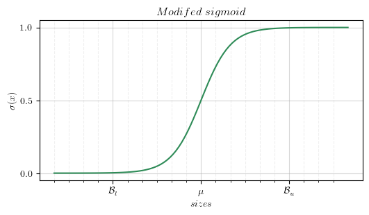
Figure 3: Function plot of $\sigma_{\mathcal{B}}(x)$.

Since the actual scale factor should be inversely proportional to the size, i.e., smaller objects need to have greater scale factors, we use a reciprocal of $r_{b}$: $r^{\prime}_{b}=\sigma_{\mathcal{B}}(-b_{sz})$, which produces 1 value when $x<\mathcal{B}_{l}$. Based on this, we define a loss function $\mathcal{L}_{scale}$ that reflects the scale factor of the single object. Note that the definition of $\mathcal{L}_{scale}$ is inspired by the binary cross entropy (BCE) loss function and the optimization is performed in two different directions at the same time: increasing scale factors for small objects and decreasing scale factors for large ones:

$$\mathcal{L}_{scale}(r^{\prime}_{\bar{b}},\phi)=-((r^{\prime}_{\bar{b}})\log(\frac{\phi}{\tau})+(1-r^{\prime}_{\bar{b}})\log(1-\frac{\phi}{\tau}))$$ (8)

where $\phi$ is the predicted scale factor from DyRA.

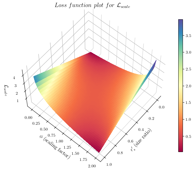
Figure 4: Loss function plot for ScaleLoss when single object. The x-axis denotes the size indicator, and the y-axis is the predicted scale factor from the network. Objects with a high indicator value will converge to a higher scale factor, while a low indicator value assists in decreasing the factor.

We visualize $\mathcal{L}_{scale}$ into a 3-D plot in Fig. 4. As intended in the definition, local minima of $\mathcal{L}_{scale}$ have been formed in the proportional relationship between the reciprocal size ratio $r^{\prime}$ and the scale factor $\phi$. $\mathcal{L}_{scale}$ is minimized when a larger $r$ leads to a decrease scale factor $\phi$ and conversely, smaller $r$ results to increase $\phi$. With an adjusted scale factor by $\tau$, the scale factor will be increased, if the obtained indicator $r^{\prime}_{\bar{b}}>0.5$, and decreasing the scale factor for $r^{\prime}_{\bar{b}}\leq 0.5$.

3.2.2 Considering Multiple Objects (ParetoScaleLoss)

When an image contains multiple objects, a suitable scale factor for an object may not be appropriate for others, due to a high variation in object sizes. The practice of averaging scale loss function values over several items may not be a feasible approach due to the potential accuracy degradation in a small number of object scales. Alternatively, we adopt the Pareto optimization [7] that can incorporate various scales as in SA-AutoAug [6]. The scale factor should be selected to minimize accuracy degradation across a set of scales $\mathbb{S}$ to enhance overall accuracy. With cumulated $\mathcal{L}_{scale}$ for a scale $i\in\mathbb{S}$, this objective can be formulated as,

$$\min_{\phi}f_{i\in\mathbb{S}}(\mathcal{L}_{scale}^{i})$$ (9)

From the MLE [33] perspective, minimizing the objective is equivalent to maximizing the likelihood of the function, which is defined as follows:

$$\max_{\phi}\mathcal{P}=\max_{\phi}\prod_{i\in\mathbb{S}}\mathcal{P}_{scale}^{i}=\max_{\phi}\prod_{i\in\mathbb{S}}e^{-f(\mathcal{L}_{scale}^{i})}$$ (10)

The difference from Eq. 9 is that each scale loss is connected by multiplication that allows maximizing likelihood in scales $\mathbb{S}$, which can allow jointly optimizing across $\mathbb{S}$.

The final ParetoScaleLoss function is defined by the log-likelihood as follows,

$$\mathcal{L}_{PS}=-\log(\mathcal{P})=-\log(\prod_{i\in\mathbb{S}}e^{-\frac{1}{|\mathbb{B}_{i}|}\sum_{\bar{b}\in\mathbb{B}_{i}}\mathcal{L}_{scale}^{\bar{b}}})$$ (11)

where $\mathbb{B}_{i}$ and $|\mathbb{B}_{i}|$ denote a set of boxes belonging to scale $i$ and the number of boxes in $\mathbb{B}_{i}$, respectively. If multiple images are in the batch, the loss is averaged as,

$$\mathcal{L}_{PS}(\theta)=-\frac{1}{|\mathbb{K}|}\sum_{\mathbb{K}}\log(\prod_{i\in\mathbb{S}}e^{-\frac{1}{|\mathbb{B}_{i}|}\sum_{\bar{b}\in\mathbb{B}_{i}}\mathcal{L}_{scale}^{\bar{b}}})$$ (12)

where $\mathbb{K}$ denotes batch. Base anchor sizes in the FPN layer are adopted as the scales $\mathbb{S}$, as a representative size of each FPN layer to increase detection possibility in the head.

3.2.3 Adjustment based on Dataset (BalanceLoss)

As stated in Sec. 3.2.1 and Sec. 3.2.2, the loss functions are formulated based on a specified range of box size, denoted $\mathcal{B}$. Specifically, the effective range of minimum and maximum size ratios are bounded by $\mathcal{B}$ in Eq. (6) and Eq. (7). In what follows, we define an additional loss function that can adaptively adjust these box size thresholds, i.e. BalanceLoss. So, we modify the definition of the range of box sizes $\mathcal{B}$, as follows, with a learnable parameter $\gamma$,

$$\mathcal{B}=\langle\mathcal{B}_{l},\mathcal{B}_{u}\rangle=\langle\gamma\cdot\mathcal{S}^{AP}_{s},\gamma\cdot\mathcal{S}^{AP}_{l}\rangle$$ (13)

where $\mathcal{S}^{AP}_{s}$ and $\mathcal{S}^{AP}_{l}$ are the threshold sizes that determine small and large objects(in AP_s and AP_l).

To find a balanced threshold that leads to an optimized scale factor even in the presence of high variances in box sizes, BalanceLoss aims to find an appropriate $\gamma$. Fig. 5 delineates the basic idea of this loss function. Let us first divide all boxes in the image into two subsets, ${\mathcal{G}}_{u}$ and ${\mathcal{G}}_{d}$, based on the average size of the threshold $\mathcal{B}_{\mu}$. To be more specific, boxes whose areas are smaller than $\mathcal{B}_{\mu}$ belong to ${\mathcal{G}}_{u}$ (in the sense that it requires up-scaling), while the others form ${\mathcal{G}}_{d}$. Then, we can compare the average of all localization loss $\mathcal{L}_{loc}$ from the original detector of boxes in each of ${\mathcal{G}}_{u}$ and ${\mathcal{G}}_{d}$. If this average was higher for ${\mathcal{G}}_{u}$, it is desirable to increase the threshold ($\mathcal{B}_{l}$) (by having a higher $\gamma$) to reduce the average of loss values for ${\mathcal{G}}_{u}$.

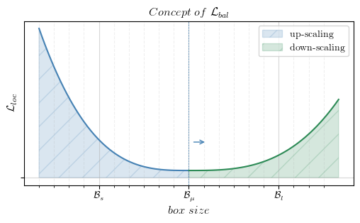
Figure 5: Concept of BalanceLoss. By the mean value of the boundary, boxes are divided into two groups: blue (to be up-scaled) and green (to be downscaled). In the figure, the mean value will be moved to enlarge the scale factor to reduce the loss value of blue because the average loss value of blue is larger than green.

Based on this intuition, we define the BalanceLoss function with the cumulated localization loss value $\mathcal{L}_{loc}^{\mathcal{G}}$ for each group $\mathcal{G}$ as follows:

$$\mathcal{L}_{bal}(\mathcal{B})=|\mathcal{B}_{\mu},\dfrac{\mathcal{F}_{norm}(\langle\dfrac{\mathcal{L}_{loc}^{\mathcal{G}_{d}}}{N_{\mathcal{G}_{d}}},\dfrac{\mathcal{L}_{loc}^{\mathcal{G}_{u}}}{N_{\mathcal{G}_{u}}}\rangle)\cdot{\langle\mathcal{M}_{l},\mathcal{M}_{u}\rangle}}{2}|_{1}$$ (14)

where $\langle\mathcal{M}_{l},\mathcal{M}_{u}\rangle$ is the boundary of $\mathcal{B}_{\mu}$ for each subset and $N_{\mathcal{G}}$ is number of boxes which belong $\langle\mathcal{G}_{d},\mathcal{G}_{u}\rangle$. After averaging the loss $\mathcal{L}_{loc}$ based on each group, this value is emphasized and adjusted by the function $\mathcal{F}_{norm}$. For emphasizing, a modified version of the Mean-Max function in Free-Anchor [51] is applied, which is sensitive within 0.1 to 0.9. We altered this function to produce respective output for each subset as,

$$\mathcal{F}_{norm}^{1}(\mathbf{x})=\dfrac{\dfrac{1}{1-x}}{\sum_{x\in\mathbf{x}}\dfrac{1}{1-x}}$$ (15)

Then, we make the obtained values as one by following the equation:

$$\mathcal{F}_{norm}^{2}(\mathbf{x})=|\mathbf{x}|\cdot x-\min(\mathbf{x})+1$$ (16)

The averaged loss value is passed sequentially to these two functions as,

$$\mathcal{F}_{norm}(x)=\mathcal{F}^{2}_{norm}(\mathcal{F}^{1}_{norm}(x))$$ (17)

After the function execution, the localization loss value is element-wise multiplied and summed with boundary $\langle\mathcal{M}_{l},\mathcal{M}_{u}\rangle$ due to the dot-product ’$\cdot$’. This operation is performed for $\mathcal{G}_{u}$ with $\mathcal{M}_{u}$ (upper boundary) and for $\mathcal{G}_{d}$ with $\mathcal{M}_{l}$ (lower boundary). If $\tilde{\mathcal{L}}_{loc}^{\mathcal{G}_{u}}$(loss value after function execution) is higher value than the $\tilde{\mathcal{L}}_{loc}^{\mathcal{G}_{d}}$, the multiplied and summed value will be shifted to $\mathcal{M}_{u}$. To modify the $\gamma$, Eq. 14 is divided by average ${S}^{AP}_{\mu}$ of $\langle\mathcal{S}^{AP}_{s},\mathcal{S}^{AP}_{l}\rangle$ as,

$$\mathcal{L}_{bal}(\mathcal{B})=|\gamma,\dfrac{\langle\tilde{\mathcal{L}}_{loc}^{\mathcal{G}_{u}},\tilde{\mathcal{L}}_{loc}^{\mathcal{G}_{d}}\rangle\cdot{\langle\mathcal{M}_{u},\mathcal{M}_{l}\rangle}}{|\mathbb{G}|\cdot{S}^{AP}_{\mu}}|_{1}$$ (18)

because of $\mathcal{B}_{\mu}=\frac{\gamma(\mathcal{S}^{AP}_{s}+\mathcal{S}^{AP}_{l})}{2}$. If $\langle\mathcal{M}_{l},\mathcal{M}_{u}\rangle$ is sufficiently large or small, the $\gamma$ will converge between two values. We select the $\langle\mathcal{M}_{l},\mathcal{M}_{u}\rangle$ as the representative size of the P4-/P6-layer to cover P3 to P7 layers of FPN.

3.2.4 Final Loss Function of DyRA

As discussed in Sec. 2, object detectors are one stage or two stages. With the designed loss functions, the total loss function for a one-stage detector is defined as follows:

$$\mathcal{L}_{total}=\mathcal{L}_{cls}+\mathcal{L}_{loc}+\mathcal{L}_{PS}+\mathcal{L}_{bal}.$$ (19)

To facilitate the joint training of DyRA and the object detector, it is desirable to associate the convergence of the loss functions of these two neural networks. So, the total loss can be modified as

$$\mathcal{L}_{total}=\mathcal{L}_{cls}+\mathcal{L}_{loc}+\mathcal{L}_{loc}\cdot(\mathcal{L}_{PS}+\mathcal{L}_{bal}).$$ (20)

In the case of two-stage detectors, each stage produces a loss, i.e., $\mathcal{L}_{loc}=(\mathcal{L}_{loc}^{1},\dots,\mathcal{L}_{loc}^{n})$, which utilized by BalanceLoss. In this case, the BalanceLoss can be redefined as follows:

$$\mathcal{L}_{bal}^{stage}=-\log(\mathcal{P}^{stage}_{bal})=-\log(\prod_{i\in stage}e^{-\mathcal{L}_{bal}^{i}})$$ (21)

to jointly reflect the output from multiple heads with the MLE form applied to ParetoScaleLoss. Therefore, the weight of BalanceLoss corresponds to each localization loss function as,

$$\tilde{\mathcal{L}}_{bal}^{stage}=-\log(\prod_{i\in stage}e^{-\mathcal{L}_{loc}^{i}\times\mathcal{L}_{bal}^{i}})$$ (22)

For ParetoScaleLoss, the weight can be obtained by the likelihood version of localization losses with the same technique from the Eq. 21. Therefore, the total loss function for the two-stage detector is defined as

$$\mathcal{L}_{total}=\mathcal{L}_{cls}+\mathcal{L}_{loc}-\log(\mathcal{P}_{loc}^{stage})\cdot\mathcal{L}_{PS}+\tilde{\mathcal{L}}_{bal}^{stage}.$$ (23)

4 Experiments

4.1 Implementation Details

We apply learning rate decay to the SGD optimizer of DyRA to prevent under-fitting; The ConstCosine schedule for a smooth learning rate transition, which combines constant and half-cosine learning rate scheduling, is employed. Multi-resolution is applied when training DyRA while maintaining an aspect ratio of (640 to 800). Within the range, the size of the shorter side is selected randomly, and we applied a maximum of 800. An anchor-based/-free multi-scale baseline is trained in 270k/180k iterations for COCO with the same data augmentation while the maximum size is 1333. DyRA is trained with 180k iterations in Sec. 4.2 for fast results with 16-image batches in a 4-GPU environment. The same training iteration from the baseline is applied for training DyRA in PascalVOC.

4.2 Accuracy Improvements

Sec. 4.2 and Sec. 4.2 show the accuracy improvements of DyRA applied to different object detectors. In most cases, the Average Precision (AP) scores have been improved by more than 1.0 points by applying DyRA, except for Mask-RCNN (with semantic segmentation). RetinaNet and FCOS on ResNet50 achieve the highest AP improvement, from 41.0% to 42.3%, by applying DyRA. To verify whether DyRA can handle various object sizes effectively, the AP scores for different object sizes are reported separately in the tables, i.e., AP_l, AP_m, and AP_s, for large, medium, and small objects, respectively. While the accuracy improvements are consistent across all sizes, the improvements tend to be larger for small objects. The biggest improvement has been observed in when DyRA is applied to Faster-RCNN with ResNet101, from 25.2% to 26.9%. The AP_m does not much increase compared to the AP_l and AP_s, due to our basic intuition, which is the scale-variant performance mainly occurs in the extreme two sides as shown in Fig. 1.

c — c — c — c c c c Model Backbone Policy AP AP_l AP_m AP_s
RetinaNet ResNet50 Baseline 36.6 49.4 40.2 20.8
(one-stage) MS baseline 38.7 50.3 42.3 23.4
MS baseline* 38.6 49.6 42.5 22.5
DyRA* 40.1 52.5 43.4 24.8
ResNet101 Baseline 38.8 50.2 42.7 21.8
MS baseline 40.4 52.2 44.4 24.0
DyRA* 41.5 53.7 45.2 25.3
Faster-RCNN ResNet50 Baseline 37.6 48.4 39.9 22.2
(two-stage) MS baseline 40.2 51.9 43.6 24.2
DyRA* 41.2 54.4 44.1 25.0
ResNet101 Baseline 39.8 52.3 43.2 23.1
MS baseline 42.0 54.6 45.6 25.2
DyRA* 43.1 57.1 46.1 26.9
Mask-RCNN ResNet50 MS baseline 41.0 53.3 43.9 24.9
(two-stage) DyRA* 41.8 54.7 44.5 26.0
ResNet101 MS baseline 43.0 56.1 46.6 26.4
DyRA* 43.6 57.8 46.8 26.3
FCOS ResNet50 MS baseline 41.0 51.7 45.3 25.0
(anchor-free) DyRA* 42.3 54.2 45.5 26.4
ResNet101 MS baseline 43.1 55.1 47.0 27.9
DyRA* 43.8 56.4 47.4 28.8

Table 1: Accuracy comparison of detectors on COCO2017. MS denotes multi-scale training, and * indicates 180k training with ConstCosine learning rate scheduling.

c — c — c — c c c c Model Backbone Policy AP AP_l AP_m AP_s
DETR ResNet50 MS baseline(150) 39.5 59.1 43.0 17.5
(transformer) DyRA 42.3 60.1 45.8 22.7

Table 2: Accuracy comparison of DETR(150 epoch results) on COCO2017.

c — c — c — c c c Model Backbone Policy AP AP_.75 AP_.5
Faster-RCNN-C4 ResNet50 MS baseline 51.9 56.6 80.3
(without FPN) DyRA* 54.4 60.0 81.1
Faster-RCNN ResNet50 MS baseline 54.5 60.5 82.1
DyRA* 56.6 62.8 82.7

Table 3: Accuracy comparison of Faster-RCNN on PascalVOC.

Sec. 4.2 shows the accuracy improvement in PascalVOC, which achieved an 2.5%/2.1% accuracy gain for non-/with-FPN model. In this experiment, DyRA can enhance the accuracy for Faster-RCNN-C4 to 54.4%, which is slightly lower AP than the MS baseline in Faster-RCNN, 56.6%. Our method can improve accuracy regardless of whether the detector incorporates an FPN or not.

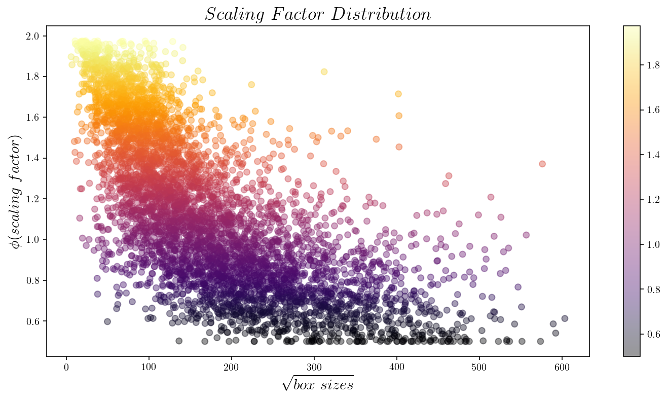
Figure 6: Distribution of scale factors achieved from the DyRA. The x-axis is the averaged box sizes within each image in the COCO2017.

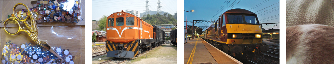
Figure 7: Example of outliers.

4.3 Analysis of Scale Factors

Fig. 6 illustrates the distribution of scale factors obtained from DyRA with respect to the averaged object sizes in the image. As intended in the definition of the ScaleLoss function (in Fig. 4), the trained image scaler produces low-scale factors for large objects and high-scale factors for small objects. In the distribution, there are a few outliers in high-scale factors for relatively large objects, examples of which are shown in Fig. 7. What all of those outliers have in common is that there is only one large single object in the image. This is because DyRA is designed to cover several objects with various sizes as elaborated in Sec. 3.2.2. As large objects are more straightforward to detect than small objects, high-scale factor values may result in large objects.

To further understand the effectiveness of scale factors, the accuracy gains achieved by DyRA compared to the MS baseline are separately illustrated for each class in Fig. 8. The y-axis is the AP improvement of DyRA over the baseline, and the x-axis indicates classes in the COCO dataset. For all detectors, the number of classes with accuracy improvements is higher than that with accuracy losses. The RetinNet has the highest number of classes with accuracy gain, while the FCOS has the lowest. However, the AP improvements are the same between the two models, while the AP_m improvement is lower in FCOS. The presence of the anchor might have caused this result because Pareto scale $\mathbb{S}$ is selected as base anchor sizes.

Figure 8: Accuracy gain of each class from DyRA trained with various detectors. Accuracy gains are achieved in almost all classes.

4.4 Adaptability to Various Image Sizes

Since the proposed technique is designed to adaptively adjust the input image taking into account the object size variations, it should also be able to properly respond to image size variations. Sec. 4.4 shows an analysis of scale factors acquired from different initial image sizes. It can be seen that the mean values of obtained scale factors are inversely proportional to the initial image sizes. This can be attributed to the fact that bigger image sizes necessitate a smaller scale factor compared to smaller image sizes. Standard deviations (Std.) of the scale factors were relatively constant over the different image sizes. Pearson correlation is acquired with scale factors obtained from training augmentation. In most sizes, the coefficient shows a high correlation, except for the smallest image size(400).

To figure out whether this tendency is reflected in accuracy, we experimented for evaluation accuracy shown in Sec. 4.4. We applied different $\tau$ values for different image sizes to get similar maximum image sizes for comparison with size=800. When we evaluate these sizes in the same model, most have similar accuracy, but the accuracy of the smallest size (400) was noticeably low compared to others. To compensate for this accuracy drop, we trained the network for size=400 with $\tau$=4 in Sec. 4.5. By having a larger $\tau$, which implies a larger scale factor range, we could improve the AP score of the smallest images up to 40. It is shown in Sec. 4.4 that this improvement is mainly attributed to the improved accuracy for medium and small objects, i.e., AP_m and AP_s. As a result, DyRA is robust to variation of input resolution when testing, as long as the size is not too small. For the extremely small image, training can match DyRA with the small image size.

c — c — c — c c c Model Image Size Pearson Correlation Mean Std.
RetinaNet 400 0.84 1.5 0.36
(ResNet50) 640 0.96 1.32 0.41
800 0.96 1.14 0.38
1200 0.94 1.06 0.37

Table 4: Analysis of scale factors from different initial image sizes ($\tau$=2) evaluated with the model trained with a maximum=800. The Pearson correlation coefficient is computed with a scale factor obtained from trained augmentation (640 to 800).

c — c c — c c c c c c Model Image size $\tau$ AP AP_.75 AP_.5 AP_l AP_m AP_s
Faster-RCNN 400 4 37.5 40.4 57.7 49.2 40.8 21.0
(ResNet50) 640 2.5 41.0 44.2 62.9 52.1 44.4 24.8
800 2 41.2 44.7 62.1 53.4 44.1 25.0
1200 1.5 41.2 44.9 62.3 53.8 44.0 24.3

Table 5: Evaluate DyRA in different initial resolutions with various $\tau$ to get a similar maximum resolution.

4.5 Effect of Balance Loss

BalanceLoss, illustrated in 3.2.3, aims to find an effective box size threshold with respect to a given dataset by determining a learnable parameter $\gamma$. Sec. 4.5 and Sec. 4.5 report the learned $\gamma$ values of DyRA. The trained $\gamma$ values were constant around 6.8 for the three detectors as shown in Sec. 4.5. This indicates that $\gamma$ is more likely to be affected by the dataset, rather than the neural network structure. The $\gamma$ value of 6.8 was obtained when it is located in the middle of the $\mathcal{M}$, which means the COCO has a Gaussian distribution. Sec. 4.5 shows the trained results with different initial values for $\gamma$. Even with different initial values, the final trained $\gamma$ values were relatively constant.

c — c c — c c c c c c Model Image size $\tau$ AP AP_.75 AP_.5 AP_l AP_m AP_s
Faster-RCNN 400 4 40.0 43.5 60.9 53.3 43.1 22.4
(ResNet50) 800 2 41.2 44.7 62.1 53.4 44.1 25.0

Table 6: Train DyRA lower resolution with larger $\tau$.

c — c Models Final $\gamma$
RetinaNet 6.82
Faster-RNN 6.80
Faster-RNN-C4 6.82

(a) Trained result of $\gamma$.

c — c c c c c c Initialization $\gamma$ Final $\gamma$
$\gamma=4$ 6.81
$\gamma=8$ 6.80

(b) Different initialization for $\gamma$ on Faster-RCNN.

(c) Training result of $\gamma$.

5 Conclusion

This paper presents a dynamic neural network called DyRA for adjusting input resolution for scale robustness against high object size variances. This network is portable to existing detectors, yielding the image-specific continuous scale factor. DyRA can be easily attached to an existing object detector as a companion neural network and can be jointly trained with it. With newly defined loss functions, DyRA can be trained to derive an adaptive scale factor that takes into account the size variance of multiple objects in a single image (ParetoScaleLoss) and the distribution of object sizes (BalanceLoss). It was shown that only by adjusting the input image resolution with the proposed technique, we could achieve AP improvements of nearly 1.0% for most detectors.

References

- Badrinarayanan et al. [2017] Vijay Badrinarayanan, Alex Kendall, and Roberto Cipolla. Segnet: A deep convolutional encoder-decoder architecture for image segmentation. IEEE transactions on pattern analysis and machine intelligence, 39(12):2481–2495, 2017.
- Beyer et al. [2023] Lucas Beyer, Pavel Izmailov, Alexander Kolesnikov, Mathilde Caron, Simon Kornblith, Xiaohua Zhai, Matthias Minderer, Michael Tschannen, Ibrahim Alabdulmohsin, and Filip Pavetic. Flexivit: One model for all patch sizes. In Proceedings of the IEEE/CVF Conference on Computer Vision and Pattern Recognition, pages 14496–14506, 2023.
- Bochkovskiy et al. [2020] Alexey Bochkovskiy, Chien-Yao Wang, and Hong-Yuan Mark Liao. Yolov4: Optimal speed and accuracy of object detection. arXiv preprint arXiv:2004.10934, 2020.
- Bolukbasi et al. [2017] Tolga Bolukbasi, Joseph Wang, Ofer Dekel, and Venkatesh Saligrama. Adaptive neural networks for efficient inference. In International Conference on Machine Learning, pages 527–536. PMLR, 2017.
- Chen et al. [2020] Yinpeng Chen, Xiyang Dai, Mengchen Liu, Dongdong Chen, Lu Yuan, and Zicheng Liu. Dynamic relu. In European Conference on Computer Vision, pages 351–367. Springer, 2020.
- Chen et al. [2021] Yukang Chen, Yanwei Li, Tao Kong, Lu Qi, Ruihang Chu, Lei Li, and Jiaya Jia. Scale-aware automatic augmentation for object detection. In Proceedings of the IEEE/CVF conference on computer vision and pattern recognition, pages 9563–9572, 2021.
- Coello [2007] Carlos A Coello Coello. Evolutionary algorithms for solving multi-objective problems. Springer, 2007.
- Cubuk et al. [2018] Ekin D Cubuk, Barret Zoph, Dandelion Mane, Vijay Vasudevan, and Quoc V Le. Autoaugment: Learning augmentation policies from data. arXiv preprint arXiv:1805.09501, 2018.
- Cubuk et al. [2020] Ekin D Cubuk, Barret Zoph, Jonathon Shlens, and Quoc V Le. Randaugment: Practical automated data augmentation with a reduced search space. In Proceedings of the IEEE/CVF conference on computer vision and pattern recognition workshops, pages 702–703, 2020.
- Dai et al. [2017] Jifeng Dai, Haozhi Qi, Yuwen Xiong, Yi Li, Guodong Zhang, Han Hu, and Yichen Wei. Deformable convolutional networks. In Proceedings of the IEEE international conference on computer vision, pages 764–773, 2017.
- Dai et al. [2020] Xin Dai, Xiangnan Kong, and Tian Guo. Epnet: Learning to exit with flexible multi-branch network. In Proceedings of the 29th ACM International Conference on Information & Knowledge Management, pages 235–244, 2020.
- Dai et al. [2021] Xiyang Dai, Yinpeng Chen, Bin Xiao, Dongdong Chen, Mengchen Liu, Lu Yuan, and Lei Zhang. Dynamic head: Unifying object detection heads with attentions. In Proceedings of the IEEE/CVF conference on computer vision and pattern recognition, pages 7373–7382, 2021.
- Everingham et al. [2010] Mark Everingham, Luc Van Gool, Christopher KI Williams, John Winn, and Andrew Zisserman. The pascal visual object classes (voc) challenge. International journal of computer vision, 88:303–338, 2010.
- Gao et al. [2019] Hang Gao, Xizhou Zhu, Steve Lin, and Jifeng Dai. Deformable kernels: Adapting effective receptive fields for object deformation. arXiv preprint arXiv:1910.02940, 2019.
- Ghiasi et al. [2019] Golnaz Ghiasi, Tsung-Yi Lin, and Quoc V Le. Nas-fpn: Learning scalable feature pyramid architecture for object detection. In Proceedings of the IEEE/CVF conference on computer vision and pattern recognition, pages 7036–7045, 2019.
- Girshick [2015] Ross Girshick. Fast r-cnn. In Proceedings of the IEEE international conference on computer vision, pages 1440–1448, 2015.
- Han et al. [2021] Yizeng Han, Gao Huang, Shiji Song, Le Yang, Honghui Wang, and Yulin Wang. Dynamic neural networks: A survey. IEEE Transactions on Pattern Analysis and Machine Intelligence, 44(11):7436–7456, 2021.
- Hao et al. [2017] Zekun Hao, Yu Liu, Hongwei Qin, Junjie Yan, Xiu Li, and Xiaolin Hu. Scale-aware face detection. In Proceedings of the IEEE Conference on Computer Vision and Pattern Recognition, pages 6186–6195, 2017.
- He et al. [2016] Kaiming He, Xiangyu Zhang, Shaoqing Ren, and Jian Sun. Deep residual learning for image recognition. In Proceedings of the IEEE conference on computer vision and pattern recognition, pages 770–778, 2016.
- He et al. [2017] Kaiming He, Georgia Gkioxari, Piotr Dollár, and Ross Girshick. Mask r-cnn. In Proceedings of the IEEE international conference on computer vision, pages 2961–2969, 2017.
- Hu et al. [2018] Jie Hu, Li Shen, and Gang Sun. Squeeze-and-excitation networks. In Proceedings of the IEEE conference on computer vision and pattern recognition, pages 7132–7141, 2018.
- Lee et al. [2019] HyunJae Lee, Hyo-Eun Kim, and Hyeonseob Nam. Srm: A style-based recalibration module for convolutional neural networks. In Proceedings of the IEEE/CVF International conference on computer vision, pages 1854–1862, 2019.
- Li et al. [2019] Yanghao Li, Yuntao Chen, Naiyan Wang, and Zhaoxiang Zhang. Scale-aware trident networks for object detection. In Proceedings of the IEEE/CVF international conference on computer vision, pages 6054–6063, 2019.
- Lin et al. [2014] Tsung-Yi Lin, Michael Maire, Serge Belongie, James Hays, Pietro Perona, Deva Ramanan, Piotr Dollár, and C Lawrence Zitnick. Microsoft coco: Common objects in context. In Computer Vision–ECCV 2014: 13th European Conference, Zurich, Switzerland, September 6-12, 2014, Proceedings, Part V 13, pages 740–755. Springer, 2014.
- Lin et al. [2017a] Tsung-Yi Lin, Piotr Dollár, Ross Girshick, Kaiming He, Bharath Hariharan, and Serge Belongie. Feature pyramid networks for object detection. In Proceedings of the IEEE conference on computer vision and pattern recognition, pages 2117–2125, 2017a.
- Lin et al. [2017b] Tsung-Yi Lin, Priya Goyal, Ross Girshick, Kaiming He, and Piotr Dollár. Focal loss for dense object detection. In Proceedings of the IEEE international conference on computer vision, pages 2980–2988, 2017b.
- Lin et al. [2023] Zhihao Lin, Yongtao Wang, Jinhe Zhang, and Xiaojie Chu. Dynamicdet: A unified dynamic architecture for object detection. In Proceedings of the IEEE/CVF Conference on Computer Vision and Pattern Recognition, pages 6282–6291, 2023.
- Liu et al. [2018] Shu Liu, Lu Qi, Haifang Qin, Jianping Shi, and Jiaya Jia. Path aggregation network for instance segmentation. In Proceedings of the IEEE conference on computer vision and pattern recognition, pages 8759–8768, 2018.
- Liu et al. [2016] Wei Liu, Dragomir Anguelov, Dumitru Erhan, Christian Szegedy, Scott Reed, Cheng-Yang Fu, and Alexander C Berg. Ssd: Single shot multibox detector. In Computer Vision–ECCV 2016: 14th European Conference, Amsterdam, The Netherlands, October 11–14, 2016, Proceedings, Part I 14, pages 21–37. Springer, 2016.
- Liu et al. [2021] Ze Liu, Yutong Lin, Yue Cao, Han Hu, Yixuan Wei, Zheng Zhang, Stephen Lin, and Baining Guo. Swin transformer: Hierarchical vision transformer using shifted windows. In Proceedings of the IEEE/CVF international conference on computer vision, pages 10012–10022, 2021.
- Liu et al. [2022] Ze Liu, Han Hu, Yutong Lin, Zhuliang Yao, Zhenda Xie, Yixuan Wei, Jia Ning, Yue Cao, Zheng Zhang, Li Dong, et al. Swin transformer v2: Scaling up capacity and resolution. In Proceedings of the IEEE/CVF conference on computer vision and pattern recognition, pages 12009–12019, 2022.
- Long et al. [2015] Jonathan Long, Evan Shelhamer, and Trevor Darrell. Fully convolutional networks for semantic segmentation. In Proceedings of the IEEE conference on computer vision and pattern recognition, pages 3431–3440, 2015.
- Maron and Lozano-Pérez [1997] Oded Maron and Tomás Lozano-Pérez. A framework for multiple-instance learning. Advances in neural information processing systems, 10, 1997.
- Park et al. [2015] Eunhyeok Park, Dongyoung Kim, Soobeom Kim, Yong-Deok Kim, Gunhee Kim, Sungroh Yoon, and Sungjoo Yoo. Big/little deep neural network for ultra low power inference. In 2015 International Conference on Hardware/Software Codesign and System Synthesis (CODES+ ISSS), pages 124–132. IEEE, 2015.
- Redmon et al. [2016] Joseph Redmon, Santosh Divvala, Ross Girshick, and Ali Farhadi. You only look once: Unified, real-time object detection. In Proceedings of the IEEE conference on computer vision and pattern recognition, pages 779–788, 2016.
- Ren et al. [2015] Shaoqing Ren, Kaiming He, Ross Girshick, and Jian Sun. Faster r-cnn: Towards real-time object detection with region proposal networks. Advances in neural information processing systems, 28, 2015.
- Singh and Davis [2018] Bharat Singh and Larry S Davis. An analysis of scale invariance in object detection snip. In Proceedings of the IEEE conference on computer vision and pattern recognition, pages 3578–3587, 2018.
- Singh et al. [2018] Bharat Singh, Mahyar Najibi, and Larry S Davis. Sniper: Efficient multi-scale training. Advances in neural information processing systems, 31, 2018.
- Tan and Le [2019] Mingxing Tan and Quoc Le. Efficientnet: Rethinking model scaling for convolutional neural networks. In International conference on machine learning, pages 6105–6114. PMLR, 2019.
- Tan et al. [2020] Mingxing Tan, Ruoming Pang, and Quoc V Le. Efficientdet: Scalable and efficient object detection. In Proceedings of the IEEE/CVF conference on computer vision and pattern recognition, pages 10781–10790, 2020.
- Tian et al. [2023] Rui Tian, Zuxuan Wu, Qi Dai, Han Hu, Yu Qiao, and Yu-Gang Jiang. Resformer: Scaling vits with multi-resolution training. In Proceedings of the IEEE/CVF Conference on Computer Vision and Pattern Recognition, pages 22721–22731, 2023.
- Tian et al. [2019] Zhi Tian, Chunhua Shen, Hao Chen, and Tong He. Fcos: Fully convolutional one-stage object detection. In Proceedings of the IEEE/CVF international conference on computer vision, pages 9627–9636, 2019.
- Wang et al. [2023] Chien-Yao Wang, Alexey Bochkovskiy, and Hong-Yuan Mark Liao. Yolov7: Trainable bag-of-freebies sets new state-of-the-art for real-time object detectors. In Proceedings of the IEEE/CVF Conference on Computer Vision and Pattern Recognition, pages 7464–7475, 2023.
- Wang et al. [2019a] Huiyu Wang, Aniruddha Kembhavi, Ali Farhadi, Alan L Yuille, and Mohammad Rastegari. Elastic: Improving cnns with dynamic scaling policies. In Proceedings of the IEEE/CVF Conference on Computer Vision and Pattern Recognition, pages 2258–2267, 2019a.
- Wang et al. [2019b] Jiaqi Wang, Kai Chen, Shuo Yang, Chen Change Loy, and Dahua Lin. Region proposal by guided anchoring. In Proceedings of the IEEE/CVF conference on computer vision and pattern recognition, pages 2965–2974, 2019b.
- Wang et al. [2017] Xin Wang, Yujia Luo, Daniel Crankshaw, Alexey Tumanov, Fisher Yu, and Joseph E Gonzalez. Idk cascades: Fast deep learning by learning not to overthink. arXiv preprint arXiv:1706.00885, 2017.
- Xie et al. [2017] Saining Xie, Ross Girshick, Piotr Dollár, Zhuowen Tu, and Kaiming He. Aggregated residual transformations for deep neural networks. In Proceedings of the IEEE conference on computer vision and pattern recognition, pages 1492–1500, 2017.
- Yang et al. [2019] Ze Yang, Shaohui Liu, Han Hu, Liwei Wang, and Stephen Lin. Reppoints: Point set representation for object detection. In Proceedings of the IEEE/CVF international conference on computer vision, pages 9657–9666, 2019.
- Zhang et al. [2022] Haotian Zhang, Pengchuan Zhang, Xiaowei Hu, Yen-Chun Chen, Liunian Li, Xiyang Dai, Lijuan Wang, Lu Yuan, Jenq-Neng Hwang, and Jianfeng Gao. Glipv2: Unifying localization and vision-language understanding. Advances in Neural Information Processing Systems, 35:36067–36080, 2022.
- Zhang et al. [2020] Shifeng Zhang, Cheng Chi, Yongqiang Yao, Zhen Lei, and Stan Z Li. Bridging the gap between anchor-based and anchor-free detection via adaptive training sample selection. In Proceedings of the IEEE/CVF conference on computer vision and pattern recognition, pages 9759–9768, 2020.
- Zhang et al. [2019] Xiaosong Zhang, Fang Wan, Chang Liu, Rongrong Ji, and Qixiang Ye. Freeanchor: Learning to match anchors for visual object detection. Advances in neural information processing systems, 32, 2019.
- Zhou et al. [2017] Hong-Yu Zhou, Bin-Bin Gao, and Jianxin Wu. Adaptive feeding: Achieving fast and accurate detections by adaptively combining object detectors. In Proceedings of the IEEE International Conference on Computer Vision, pages 3505–3513, 2017.
- Zhu et al. [2018] Lei Zhu, Zijun Deng, Xiaowei Hu, Chi-Wing Fu, Xuemiao Xu, Jing Qin, and Pheng-Ann Heng. Bidirectional feature pyramid network with recurrent attention residual modules for shadow detection. In Proceedings of the European Conference on Computer Vision (ECCV), pages 121–136, 2018.
- Zhu et al. [2021] Mingjian Zhu, Kai Han, Enhua Wu, Qiulin Zhang, Ying Nie, Zhenzhong Lan, and Yunhe Wang. Dynamic resolution network. Advances in Neural Information Processing Systems, 34:27319–27330, 2021.
- Zhu et al. [2019] Xizhou Zhu, Han Hu, Stephen Lin, and Jifeng Dai. Deformable convnets v2: More deformable, better results. In Proceedings of the IEEE/CVF conference on computer vision and pattern recognition, pages 9308–9316, 2019.