Improved Prototypical Semi-Supervised Learning with Foundation Models: Prototype Selection, Parametric vMF-SNE Pretraining and Multi-view Pseudolabelling

Abstract

In this paper we present an improved approach to prototypical semi-supervised learning for computer vision, in the context of leveraging a frozen foundation model as the backbone of our neural network. As a general tool, we propose parametric von-Mises Fisher Stochastic Neighbour Embedding (vMF-SNE) to create mappings with neural networks between high-dimensional latent spaces that preserve local structure. This enables us to pretrain the projection head of our network using the high-quality embeddings of the foundation model with vMF-SNE. We also propose soft multi-view pseudolabels, where predictions across multiple views are combined to provide a more reliable supervision signal compared to a consistency or swapped assignment approach. We demonstrate that these ideas improve upon Predicting View-Assignments with Support Samples (PAWS), a current state-of-the-art semi-supervised learning method, as well as Robust PAWS (RoPAWS), over a range of benchmarking datasets. We also introduce simple $k$-means prototype selection, a technique that provides superior performance to other unsupervised label selection approaches in this context. These changes improve upon PAWS by an average of +2.9% for CIFAR-10 and +5.7% for CIFAR-100 with four labels per class, and by +15.2% for DeepWeeds, a particularly challenging dataset for semi-supervised learning. We also achieve new state-of-the-art results in semi-supervised learning in this small label regime for CIFAR-10 — 95.8% (+0.7%) and CIFAR-100 — 76.6% (+12.0%).

1 Introduction

Training neural networks with small amounts of labelled data is of considerable practical interest, as annotating large image datasets is an expensive and tedious exercise. Within the field of computer vision, semi-supervised learning approaches are often used to tackle this challenge by leveraging a large scale set of unlabelled data to learn better models, with only a small annotated dataset [38].

While semi-supervised learning approaches have seen great success, they also require much more computing power compared to supervised learning approaches [1, 35]. Using self-supervised learning to pre-train neural networks and employ transfer learning is an emerging solution to this challenge [5, 10]. The recent push to develop foundation models within the computer vision field is of particular interest [48]. These are trained on large datasets over numerous different image domains with the aim of building a model that produces useful visual representations for any task [26].

This paradigm mirrors the biological context, where it has been shown that the ability of humans to quickly learn new concepts from sparse examples relies on adapting previously learnt representations [33]. However, most semi-supervised computer vision approaches within the literature are designed to be trained from scratch, rather than utilise a pre-trained foundation model [1, 35, 42].

In this work, we explore how the Predicting View-Assignments with Support Samples (PAWS) semi-supervised learning approach can be efficiently and effectively trained using a foundation model as a backbone over a wide range of datasets. We refer to PAWS as a prototypical method because the labelled images are used to generate prototype vectors, which are used to make predictions [45]. This method is computationally more efficient to train and offers similar or better accuracy compared to other semi-supervised learning frameworks [1].

We identify three challenges in using PAWS with foundation models, and in each case propose solutions to improve performance

• Randomly initializing the projection head, which is used after the neural network backbone to make predictions in PAWS, can result in poor performance for some datasets. This can be solved by using the novel parametric vMF-SNE pretraining approach presented in this work.

• The consistency loss used in PAWS can degrade model performance over a training run. By combining predictions of multiple augmented views of an image to create soft multi-view pseudolabels, we can generate a higher quality supervision signal [3] and train more accurate models.

• Randomly selecting prototype images for the labelled dataset, even when stratifying by class, can result in poor performance. We propose the simple $k$-means prototype selection strategy, that outperforms other state-of-the-art unsupervised label selection methods [40].

We use the recently released DINOv2 [26] foundation model for this work, and for the fairest possible comparison to previous results we employ the smallest ViT-S/14 distilled model as the frozen backbone, where we do not optimise the weights during training. Using the techniques presented in this paper, we are able to outperform the original PAWS approach on several benchmarking datasets, including by an average of +2.9% on CIFAR-10 with 40 labels and by +5.7% on CIFAR-100 with 400 labels. We demonstrate these changes also improve upon the performance of RoPAWS [23], an approach which modifies the PAWS loss to enable more effective learning from uncurated data. We also beat prior state-of-the-art performance for semi-supervised learning on these datasets where comparisons are available.

2 Related Work

2.1 Self-supervised learning and foundational models

Within the field of computer vision, self-supervised learning approaches create a mapping from the image domain to a representation space that captures the semantic content of the image with minimal loss of information. The degree to which semantic content is retained can be tested by undertaking downstream tasks within the representation space, such as image classification, segmentation and object detection [30]. This mapping is defined by a neural network $f_{\theta}:X\in\mathbb{R}^{3\times H\times W}\to Z_{1}\in\mathbb{R}^{d_{1}}$ and the representation space $Z_{1}$ can also be referred to as a latent space. Here $H$ and $W$ are the height and width of the input images, and $d_{1}$ is the dimensionality of this representation space.

Neural networks can be effectively trained in a self-supervised fashion using a contrastive loss. SimCLR [10] is one of the most effective contrastive methods, where a neural network is trained to identify pairs of augmented images within a large mini-batch. Other approaches have also seen success, such as Bootstrapping [15, 8], where one neural network learns to predict the output of another from a different augmented view, and image masks [2, 49], where models are trained to make consistent inferences from masked inputs.

These methods rely on similar principles — training a neural network to map corrupted versions of an image or image patches to similar locations in the latent space. A projection head is commonly employed in this context, which is defined by the neural network $g_{\phi}:Z_{1}\in\mathbb{R}^{d_{1}}\to Z_{2}\in\mathbb{R}^{d_{2}}$, which creates a second latent space $Z_{2}$ with dimension $d_{2}$. This allows the self-supervised loss to be calculated in this second space, so that it does not compromise the utility of the embeddings within the first latent space $Z_{1}$. It is found that using $Z_{2}$ directly for downstream tasks leads to poorer performance [11].

Models trained using these approaches show strong generalisability to previously unseen image tasks [10], and this has led to the development and release of foundation vision models trained on large amounts of data with these techniques. Recently, DINO-V2, a foundation model trained on 142 million images using a combination of boostrapping and masking approaches, was able to achieve an accuracy of 86.7% accuracy on ImageNet with a linear classifier [26].

2.2 Semi-supervised learning and PAWS

Semi-supervised learning approaches train a model that performs a particular task, such as image classification, using a small set of labelled data $D_{l}$ and a much larger set of unlabelled data $D_{u}$. By taking into account the distribution of the unlabelled data within the learning process, semi-supervised methods can train much more accurate models compared to supervised approaches within this context [38].

Strategies from self-supervised learning have inspired advances within this space. PAWS [1] takes inspiration from elements within SwAV [7] and BYOL [15]. These include using a consistency loss, which is similar to bootstrapping, where the neural network is trained to provide similar predictions for different augmented views of an image. PAWS also adapts the idea of prototypes from SwAV, but instead of learning prototype vectors, the embeddings of the labelled images in $D_{l}$ are employed. This is a unique take on the idea of prototypes, as these are usually learned in a non-parametric fashion [7, 45].

Following Mo et al. [23], PAWS can be written down as a generative model. The probability density of a sample from the dataset is defined using the prototypes $D_{l}$ and a similarity kernel,

$$p(x_{j}|D_{l}) :=\frac{1}{|D_{l}|}\sum_{x_{i}\in D_{l}}k_{Z_{2}}(x_{j};x_{i})$$ (1)

where the similarity kernel is defined by

$$k_{Z_{2}}(x_{j};x_{i}) =\frac{1}{Z}\text{exp}\left(z^{\prime}_{j}\cdot z^{\prime}_{i}/\tau\right)$$ (2)

$$z^{\prime} =\frac{g_{\phi}(f_{\theta}(x))}{||g_{\phi}(f_{\theta}(x))||}$$ (3)

with $Z$ a normalizing constant. PAWS defines this conditional probability within the second latent space $Z_{2}$, employing the projection head $g_{\phi}$.

For a particular class $y$, we can use the set of prototypes $B_{y}=\{x_{i}\in D_{l}|y_{i}=y\}$ to define the support of that image conditional on $y$ as

$$p(x_{j}|y,D_{l}): =\frac{1}{|B_{y}|}\sum_{x_{i}\in B_{y}}k_{Z_{2}}(x_{j};x_{i})$$ (4)

and through Bayes’ rule, we can derive the predicted class probabilities as

$$p(y|x_{j},D_{l}) =\frac{p(x_{j}|y,D_{l})p(y)}{p(x_{j}|D_{l})}$$ (5)

$$=\sigma\left(z_{i}\cdot z_{S}^{T}/\tau\right)y_{S}=p_{j}$$ (6)

where $y_{S}$ is the corresponding one-hot or soft labels corresponding to the classes of the prototypes, $\tau$ is a temperature hyperparameter and $\sigma$ is the softmax function. Finally, $z_{S}$ is the matrix of latent representations of the prototypes. Eq. 7 sets $p(y)=\frac{1}{C}$ and $B_{y}=N/C$, which creates a prior that assumes class balance in the data and prototypes.

To train the models using a consistency loss, PAWS employs cross-entropy to encourage the prediction of two views of the same image to be similar, with

$$L_{paws}=\frac{1}{2n}\sum_{i=1}^{n}\left(H(\rho(p_{i}^{+}),p_{i})+H(\rho(p_{i}),p_{i}^{+})\right)-H(\overline{p})$$ (7)

where $n$ is the number of unlabelled images, $\rho$ is a sharpening function used to prevent representation collapse, and $\overline{p}$ is the average sharpened predictions on the unlabelled images. This is used to maximise the entropy of the predictions in the last term. This helps ensure that the association of the unlabelled points with each label is more uniform, and is referred to as the mean entropy maximization regularization term [1].

2.3 Stochastic neighbour embeddings

Stochastic Neighbour Embeddings (SNE) [18] solve a similar problem to self-supervised learning, but in a more general domain. Given a high dimensional dataset, SNE methods create a representation of this data in different dimensional space while attempting to ensure the relationship between items in the dataset is preserved. They are often used for plotting high dimensional data in lower dimension spaces [41]. One of the most well-known and commonly used is the t-distributed Stochastic Neighbour Embedding (t-SNE) approach [37].

For a given set of high dimensional points, t-SNE attempts to learn a lower dimensional embedding by minimizing the KL-divergence between distributions defined in the higher ($\mathbb{R}^{P}$) and lower ($\mathbb{R}^{Q}$) dimensional spaces. First, probabilities are computed in the high dimensional space that are proportional to the similarity of the objects using a multidimensional Gaussian distribution as a kernel

$$p_{j|i} =\frac{k_{P}(x_{j};x_{i})}{\sum_{k\not=i}k_{P}(x_{k};x_{i})}$$ (8)

$$k_{P}(x_{j};x_{i}) =C_{p}(\sigma_{i})\text{exp}\left(-||x_{i}-x_{j}||^{2}/2\sigma_{i}^{2}\right)$$ (9)

where $p_{i|i}=0$ and $C_{p}(\sigma_{i})$ is a normalization constant. The bandwidth of the Gaussian kernel $\sigma_{i}$ is determined using the bisection method to ensure that the entropy of the conditional distribution equals a predefined constant, which is call the perplexity hyperparameter. This means that each point has a similar number of ”close” points, or nearest neighbours within this distribution, as smaller values of $\sigma_{i}$ are used in denser regions of space.

To make a symmetric distribution, $P$ is defined as

$$p_{ij}=\frac{p_{j|i}+p_{i|j}}{2N}$$ (10)

where $N$ is the number of data points.

For the lower dimensional distribution $Q$, similarities are measured using a similar approach with the student $t$-distribution

$$q_{ij} =\frac{k_{Q}(z_{j};z_{i})}{\sum_{k}\sum_{i\not=k}k_{Q}(z_{k};z_{i})}$$ (11)

$$k_{Q}(z_{j};z_{i}) =C_{q}\left(1+||z_{i}-z_{j}||^{2}\right)^{-1}$$ (12)

where $q_{ij}=0$ and $C_{q}$ normalizes the distribution. The loss for this problem is given by the KL-divergence of the $P$ and $Q$ distributions

$$\text{KL}(P||Q)=\sum_{i\not=j}p_{ij}\log\frac{p_{ij}}{q_{ij}}$$ (13)

where the $z\in\mathbb{R}^{Q}$ points are optimised to minimise the KL-divergence using a gradient descent approach.

One of the challenges in using this approach is that it learns a non-parameteric mapping. Although there are some tricks that can be employed, new points cannot be directly mapped into the learned lower dimensional space [19].

An alternative method, known as parametric t-SNE [36], uses a neural network to learn a mapping function from the high dimensional space to the low dimensional space. In this context, the neural network weights are optimized using gradient descent on Eq. 13, instead of the lower dimensional coordinates.

2.4 Prototype selection strategies

The goal of prototype selection is to choose from a dataset $D$ with no label information the most informative set of images $D_{l}^{*}$ with which to label and undertake semi-supervised, active or few-shot learning. Other works have referred to this challenge as unsupervised selective labelling[40], or the cold start problem [9]. The most informative image set is defined as the set of images for a given budget of $|D_{l}|$, that obtain maximal performance under a given learning paradigm. While it has been found that using these prototypical image sets can lead to significant performance improvements [6, 35, 42], identifying them can be challenging, particularly within an unsupervised context.

The Unsupervised Selective Labelling (USL) approach is the the current state-of-the-art method for unsupervised prototype selection when using a frozen backbone, such as a self-supervised or foundation model [40]. This approach uses the density of the data within the latent space $Z_{1}$ as a primary indicator of informativeness. In other words, samples in denser areas of space are assumed to be more informative. However, this definition encounters problems when selecting a set of images, as many of the selected prototypes are similar. To mitigate this, the USL approach uses $k$-means clustering to seperate the dataset into clusters, samples the densest regions within each cluster and then regularize the point set using the inverse distance between samples to obtain a more diverse prototype set.

3 Methodology

3.1 Parametric von-Mises Fisher Stochastic Neighbour Embedding

If we are using a pretrained backbone model $f_{\theta}$, which provides a good representation of our data in the latent space $Z_{1}$, a good starting point for our projection head $g_{\phi}$ should reflect the local structure of $Z_{1}$ within $Z_{2}$. In other words, images mapped to locations close to each other in $Z_{1}$ should ideally also be close in $Z_{2}$. This is not a given if we randomly initialize the parameters $\phi$, and without placing restrictions on the architecture of $g$ and the dimensionality of $Z_{1}$ and $Z_{2}$, we cannot simply initialise $g_{\phi}$ as an identity mapping.

A potential solution is to pretrain our projection head using an SNE approach, as these methods are designed to address this challenge. While, regular $t$-SNE cannot be used directly as it is a non-parametric approach [19], we can use a parametric t-SNE [36] inspired method instead to learn a mapping using our projection head $g$. This is similar to amortized methods used in other contexts, where functional mappings of parameters are learned instead of the parameters themselves [34].

However, we do not necessarily wish to map our data into a lower dimensional space. In PAWS, it can be that $Z_{2}$ is of a higher or equal dimension compared to $Z_{1}$. To select a more appropriate set of distributions to use in this case, we observe that within the probablistic perspective of PAWS in Eq. 2, the kernel used is a von-Mises Fisher (vMF) distribution,

$$k^{\prime}_{Z_{2}}(x_{j};x_{i}) =C_{p}(1/\tau)\text{exp}\left(z^{\prime}_{j}\cdot z^{\prime}_{i}/\tau\right).$$ (14)

In high dimensions, the normalizing constant $C_{p}$ can be approximated with a smooth differentiable function [14], but that is not necessary for this work. This provides a natural distribution to work with for this problem, which has been used previously in a non-parametric SNE context [39]. Here we present a parametric version of the vMF-SNE approach.

For the latent space defined by our backbone model $f_{\theta}$, we can define

$$p^{\prime}_{j|i} =\frac{k_{Z_{1}}(x_{j};x_{i})}{\sum_{k\not=i}k_{Z_{1}}(x_{k};x_{i})},$$ (15)

$$k_{Z_{1}}(x_{j};x_{i}) =C_{p}(\kappa_{i})\text{exp}\left(z_{j}\cdot z_{i}\kappa_{i}\right),$$ (16)

$$z =\frac{f_{\theta}(x)}{||f_{\theta}(x)||}.$$ (17)

We set $\kappa_{i}$ for each point to ensure that the entropy equals a predefined constant, $H_{i}=\sum_{k}p_{k|i}\log p_{k|i}=\gamma$, where $\gamma$ is the perplexity parameter. For each point, $\kappa_{i}$ is determined using the bisection method. To obtain a symmetric distribution, we calculate $p_{ij}$ as done in Eq. 10.

For the latent space $Z_{2}$, a vMF distribution with constant variance is used,

$$q^{\prime}_{j|i} =\frac{k_{Z_{2}}(x_{j};x_{i})}{\sum_{k\not=i}k_{Z_{2}}(x_{k};x_{i})}$$ (18)

where $k_{Z_{2}}$ is the PAWS kernel in Eq. 2.

We also symmetrise this conditional distribution as above to obtained $q_{ij}$. We can then use the KL-divergence as a loss function,

$$\text{KL}(Q^{\prime}||P^{\prime})=\sum_{ij}p^{\prime}_{ij}\log\frac{p^{\prime}_{ij}}{q^{\prime}_{ij}}$$ (19)

and take gradients of this loss with respect to the parameters of the projection head $g_{\phi}$, as in parametric t-SNE [36]. This allows us to train $g_{\phi}$ using a similar learning approach as with PAWS, utilising mini-batching, LARS-SGD [47], and image augmentations.

This defines a self-supervised method, provided a frozen backbone model $f_{\theta}$, where we take the local structure of the latent space $Z_{1}$ from the backbone model and map it into $Z_{2}$, the latent space defined by the projection head. There are three key hyper-parameters in this process — the batch size, which defines the number of images to sample in each mini-batch, the perplexity parameter $\gamma$, and the concentration of the vMF distributions in $Z_{2}$ which is determined by $\tau$. An ablation study considering the impact of these parameters is presented in the supplementary material.

3.2 Multi-view pseudolabelling

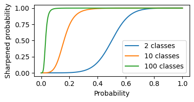
Figure 1: Impact of sharpening approach in PAWS on the class probability. We show the impact of sharpening on the probability of the first class when $T=0.25$ in Equation 20, with the probability of all other classes set to be equal.

The loss function used by PAWS in Eq. 7 is presented by Assran et al. [1] as a consistency based loss, where the method is penalised by the prediction from one augmented view of an image differing from another. However, they use a sharpening function within this loss to prevent representational collapse. The sharpening function they use is defined by

$$\rho(p)_{i} =\frac{p_{i}^{1/T}}{\sum_{i=1}^{C}p_{i}^{1/T}}$$ (20)

with $T=0.25$. For moderately confident predictions, this level of sharpening very quickly leads to an entirely confident sharpened prediction (Figure 1). This means that even if the network makes similar, only mildly confident predictions for two augmented views of an image, the sharpening approach that is employed means the loss will be large in this instance and behave like a pseudo-labelling approach. This behaviour becomes more extreme when the classification problem has a larger amount of classes.

We have observed that this can degrade model performance over a training run, and propose that combining predictions from multiple views can give more robust pseudolabels [3] and improve accuracy. The original PAWS approach takes two global views, and six local views of each unlabelled image in a mini-batch. We propose to jointly sharpen the two global views together

$$\rho(p_{1},p_{2})_{i} =\frac{(p_{1i}p_{2i})^{1/2T}}{\sum_{i=1}^{C}(p_{1i}p_{2i})^{1/2T}}$$ (21)

to create the pseudolabelling PAWS loss

$$L_{pseudo-paws}= \frac{1}{2n}\sum_{i=1}^{n}\left(H(\rho(p_{i},p_{i}^{+}),p_{i})\right.$$

$$+\left.H(\rho(p_{i},p_{i}^{+}),p_{i}^{+})\right)-H(\overline{p}).$$ (22)

This change does not introduce any risk of representational collapse, as sharpening is still employed to ensure that the target $\rho(p_{i},p_{i}^{+})$ is not equal to the uniform distribution [1].

3.3 Simple $k$-means prototype selection

Previous prototype selection approaches, such as USL [40], have considered the density of the data within the latent space to be an indicator of informativeness. In t-SNE, a perplexity parameter is used to normalise the density of the high dimensional space to visualize points in a low dimensional setting in a semantically meaningful way [37]. This suggests that density might not be the most important consideration and in this work we propose the simple $k$-means prototype selection strategy. This approach provides for a more diverse sampling of prototypes in three steps

1. Calculate the normalized embeddings for the images in the dataset $D$ using the foundation model, to obtain the normalized representation of this data in the latent space $Z_{1}$.

2. Undertake $k$-means clustering to determine the $|D_{l}|$ centroids for each cluster.

3. Identify the image closest to each centroid. Label these images and use them as the prototypes in $D_{l}^{*}$ for semi-supervised learning.

We choose $k$-means clustering for the second step as it is fast to compute and allows for the selection of a fixed number of clusters centroids. This algorithm clusters a dataset into $k$ sets $S$, such that the within cluster sum of squares is minimised [21]

$$\text{arg min}_{S}\sum_{i=1}^{k}\sum_{z\in S_{i}}||z_{i}-\mu_{i}||^{2}$$ (23)

where $\mu_{i}$ is the centroid of the points in $S_{i}$. By normalizing the image embeddings $z\in Z_{1}$ in the first step, the squared euclidean distance becomes proportional to cosine distance, which is often used for determining image similarity [26, 29]. In this sense, we can interpret our simple $k$-means prototype selection procedure as identifying clusters of visually similar images, and selecting the most representative image from each cluster as a prototype.

4 Implementation details

Throughout this work we freeze the parameters of the backbone DINOv2 ViT-S/14 distilled foundation model that is used. This makes model training require fewer computational resources. In constrast to the base PAWS approach, we do not train prediction heads and only report results using the inference formula in Eq. 6 using prototypes. Otherwise, we closely follow the implementation of PAWS [1] and RoPAWS [23] for our experiments. Further details and hyperparameters are provided in the supplementary material.

5 Main Results

5.1 Datasets

We select seven datasets to demonstrate our approach. These include CIFAR-10 (10 classes), CIFAR-100 (100 classes) [20], EuroSAT (10 classes) [16], Flowers-102 (102 classes) [24], Food-101 (101 classes) [4], Oxford Pets (37 classes) [27] and DeepWeeds (2 classes) [25]. While DeepWeeds has originally 9 classes, we treat it as a binary classification problem to identify weeds versus not weeds, due to the size of the negative class.

When reporting our results, we choose the best validation epoch and report the test accuracy if available. Otherwise we report the best validation accuracy. For EuroSAT and DeepWeeds, where preset validation splits were not available, we sampled 500 images per class, and 30% of the images for the 9 original classes respectively. When sampling the prototypes for semi-supervised learning, we selected 4 (CIFAR-10), 4 (CIFAR-100), 4 (EuroSAT), 27 (DeepWeeds - binary), 2 (Flowers-102), 2 (Food-101) and 2 (Oxford Pets) images per class. Results are reported as the mean of five runs and the standard deviation, with the same sets of prototypes being used for all experiments unless specified otherwise.

5.2 Pretraining with vMF-SNE

Feature	C10	C100	EuroSAT	DeepWeeds	Flowers	Food	Pets
DINOv2 ViT-S/14 backbone	96.2	82.3	90.0	88.7	99.3	80.9	91.5
+ vmf-SNE projection head	96.3±0.1	78.9±0.1	91.9±0.1	91.3±0.1	98.5±0.4	81.0±0.1	93.0±0.1

Table 1: Performance of vMF-SNE approach for pre-training projection heads. We report the kNN performance [43] for our vMF-SNE approach for pretraining projection heads, in comparison to the backbone it was trained to reproduce the local structure for. In six of eight cases, we obtain similar or better kNN performance for the projection head compared to the foundation model backbone using our vMF-SNE approach.

In a classification context, the performance of the backbone model can be measured non-parametrically using a weighted k-Nearest Neighbor (kNN) Classifier [43]. This provides for a quantitative approach to measure the performance of the projection head trained using vMF-SNE, as reproducing the local structure of the backbone model should provide similar kNN accuracy. We find that for six of the eight datasets considered, we can meet or beat the kNN accuracy of the backbone model through vMF-SNE pretraining (Tab. 1).

5.3 Combining vMF-SNE pretraining and multi-view pseudolabelling

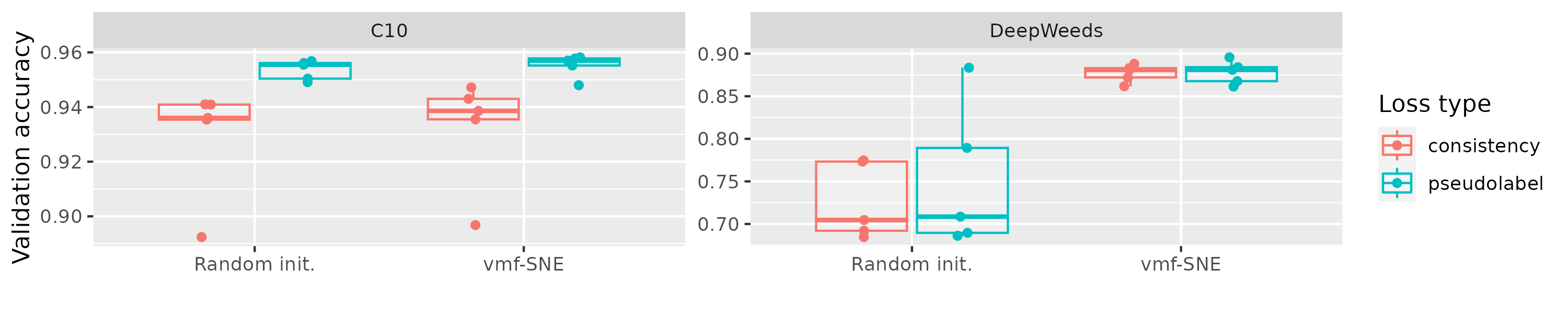
(a) Best validation accuracy

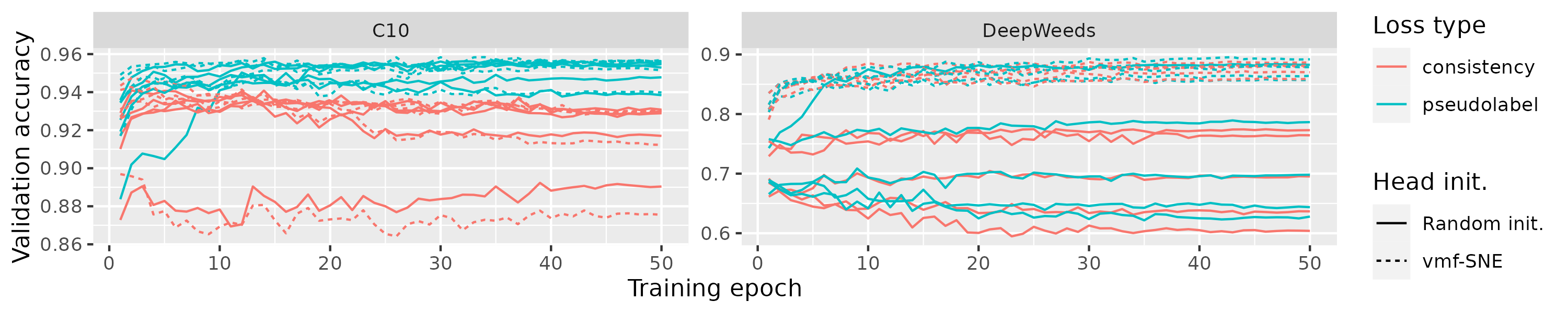
(b) Learning curves

Figure 2: Comparison of vMF-SNE and multi-view pseudolabelling versus the original implementation of PAWS. We compare the base PAWS method with pretraining from a vMF pretrained projection head, using multi-view pseudolabelling, and combining these two approaches together. Neither method appears to hurt performance, but using multi-view pseudolabelling results in better CIFAR-10 models, and vMF-SNE pretraining results in better DeepWeeds models.

Head init.	Loss type	C10	C100	EuroSAT	DeepWeeds	Flowers	Food	Pets
State of the art		95.1 [42]	64.64 [46]
Random init.	consistency	92.9±2.1	70.9±1.5	94.4±0.3	72.6±4.5	98.5±0.7	75.1±2.0	90.2±1.0
vmf-SNE	pseudolabel	95.5±0.4	73.6±1.2	94.4±0.2	87.8±1.4	98.9±0.4	75.5±2.5	91.6±0.2

Table 2: Performance of vMF-SNE and multi-view pseudolabelling versus the original implementation of PAWS on several benchmarking datasets. We find that for EuroSAT we obtain similar results to the base PAWS approach, but in all seven other cases more accurate models are trained with our method.

We start with small scale experiments to determine if vMF-SNE pretraining improves the performance of models trained with the regular PAWS loss, and if performance improves when using multi-view pseudolabelling. For CIFAR-10 we find that the multi-view pseudolabelling improves accuracy by about 2%, while for DeepWeeds vMF-SNE pretraining improves accuracy by more than 10% (Fig. 2(a)). For CIFAR-10, we see a small performance improvement for using vMF-SNE pretraining, and for DeepWeeds we obtain similar results between consistency and multi-view pseudolabelling.

It is noted that the performance improvement from vMF-SNE pretraining is not due to a head-start in training. While it does provide a better starting point for learning, in both cases we train models until they completely converge, and vMF-SNE pretrained projection heads converge to higher performing maxima (Fig. 2(b)). We also observe that for CIFAR-10, using the consistency loss results in runs degrading in performance after about ten epochs. When using multi-view pseudolabelling, the validation accuracy remains stable once the models have converged.

The performance of PAWS with our methodological improvements versus the base approach are shown in Tab. 2 for all seven datasets. For EuroSAT we obtain similar results, but every other case using vMF-SNE pretraining and multi-view psuedolabelling outperforms the baseline.

5.4 Prototype selection approaches

Head init.	Loss type	Label selection Strat.	C10	C100	Food
vmf-SNE	pseudolabel	Random Strat.	95.5±0.4	73.6±1.2	75.5±2.5
Random init.	consistency	USL	93.6±0.4	74.4±0.6	*
Random init.	consistency	Simple $k$-means	94.4±0.5	74.8±0.3	80.7±0.4*
vmf-SNE	pseudolabel	USL	95.0±0.4	76.3±0.5	*
vmf-SNE	pseudolabel	Simple $k$-means	95.8±0.1	76.6±0.3	81.5±0.7*

Table 3: Base PAWS approach versus our improvements and employing prototype selection strategies. It is found that using prototype selection strategies provides performance improvements in comparison to a random stratified sample, particularly when our vMF-SNE pretrained projection heads and multi-view pseudolabelling techniques are employed. The simple $k$-means prototype selection strategy also outperforms USL [40] on these datasets. *We only report results for label sets where atleast 100 classes were chosen for the Food101 dataset. This was four out of five runs for the simple $k$-means approach and zero for the USL approach, so it is left blank. See supplementary material for further details.

Depending on the prototype set chosen, the results from semi-supervised learning with a small numbers of prototypes can be highly variable [6]. This phenomenon is responsible for much of the variance observed in Tab. 2.

We compare two approaches to choose a more optimal set of prototypes compared to a class-based random stratified sample. These are the unsupervised selective labelling (USL) procedure introduced by Wang et al. [40], and our simple $k$-means prototype selection strategy. It is found that this second method produces improved results, particularly for cases where our vMF-SNE pretraining and multi-view pseudolabelling are employed (Tab. 3).

5.5 Transfer learning

Head init.	DeepWeeds
Random init.	75.1±8.5
vmf-SNE on C100	75.9±7.2
vmf-SNE on C10	77.4±6.3
vmf-SNE on Food	84.1±5.6
vmf-SNE on DeepWeeds	87.8±1.4

Table 4: Transferability of vMF-SNE pretraining between datasets. It is found that pretraining projection heads with vMF-SNE obtains better results over random intialisation, even if the dataset used for pretraining differs from that on which the task is being learned.

Pretraining a projection head using our vMF-SNE approach before training can be cumbersome, so we undertook a small experiment to explore if there is the potential for transfer learning to be employed. We found that this is likely to be the case, as projection heads trained on different datasets appear to perform better than random initialisation as shown in Tab. 4.

5.6 Compatability with RoPAWS

Head init.	Loss type	C10	DeepWeeds
Random init.	consistency	93.3±1.5	81.2±6.8
vmf-SNE	pseudolabel	95.5±0.3	86.2±0.8

Table 5: Applying vMF-SNE pretraining and multi-view pseudolabelling with the RoPAWS loss. It is found that our approach also improves the performance in the case of using the RoPAWS loss [23].

The changes proposed in this paper to PAWS are also compatible with RoPAWS [23]. In our experiments we have found that vMF-SNE pretraining and multi-view pseudolabelling improves the performance obtained when training RoPAWS on in-distribution data (Tab. 5). This suggests that the characteristics of PAWS that leads to poor performance on DeepWeeds and with the consistency loss on CIFAR-10, also hold for RoPAWS.

6 Discussion

By introducing parametric vMF-SNE pretraining, multi-view psuedolabelling and simple $k$-means prototype selection, we find that improved performance can be achieved with PAWS [1] and RoPAWS [23], and using DINOv2 foundation models [26] we can obtain new state-of-the-art results for several semi-supervised classification benchmarks. This approach is also computationally efficient, through the use of the frozen foundation model backbone. All of the models reported in this paper were only trained for 50 epochs, and our vMF-SNE pretraining runs only required 20 epochs. This meant that even for the Food-101 dataset with 75,000 images, training a single model took less than two hours with two Nvidia V100 graphics cards.

We obtain state-of-the-art semi-supervised performance using a prototype based approach, making predictions using the approach in Eq. 6 [43, 1]. This classifier can be seen as a vMF mixture model [32] in the latent space, where each prototype represents a component of the mixture with equal concentration. A similar prediction method is employed in the CLIP multi-modal approach, where text embeddings are used to define classes in a zero-shot fashion [29]. Similar approaches are also used to train models that are robust to adversarial examples and perform well on identifying out-of-distribution examples [13, 22]. Further work will consider if these properties also extend to the learning framework considered here.

Knowledge distillation [17] serves a similar purpose to parametric vMF-SNE pretraining. In the classic formulation of knowledge distillation, the predicted softmax class probabilities of the final layer are calculated using a logit based approach

$$p_{\text{logit}}(y_{i}|x)=\frac{\text{exp}(z_{i}(x)/t)}{\sum_{j}\text{exp}(z_{j}(x)/t)}$$ (24)

where $z_{i}$ is the logit of the last layer that corresponds to class $y_{i}$, using a high temperature $t$. Then, the loss is given by the crossentropy,

$$\mathcal{L}_{\text{distillation}}=-\sum_{j}^{n}\sum_{i}\hat{p}(y_{i}|x_{j})\log p(y_{i}|x_{j})$$ (25)

between the teacher model prediction $\hat{p}$ and the student model prediction $p$. Minimizing this loss trains the student network to predicts the same outputs as the teacher on augmented views. The DINOv2 ViT-S/14 distilled foundation model was trained using this approach, with the teacher model being the ViT-G/14 model that was trained using self-supervised learning. However, the head of the DINOv2 models are not used for inference, and the backbone features of the distilled model can be quite different from the teacher [26]. The parametric vMF-SNE method introduced in this paper could provide for an alternative approach to knowledge distillation in this context.

With the release of ChatGPT vision by OpenAI, it is possible that many vision tasks may be able to be completed by multi-modal large language models (mm-LLM) in a zero-shot or few-shot fashion. For the foreseeable future at least, we believe this work will remain relevant as mm-LLMs are computationally intensive to deploy and query. In comparison, the vision models trained in this paper can undertake spefic visual tasks with greater throughput and require less computing power to train. The simple $k$-means prototype selection approach could even be used to identify small optimal prototype sets, which could be labelled by an mm-LLM and easily curated.

Supplementary Material

7 Implementation details

7.1 PAWS

We adapted the PAWS and RoPAWS PyTorch [28] implementation available at this GitHub repository to our own codebase using PyTorch-Lightning [12] and Hydra [44], which we ensured produced identical results. We employed the same samplers, optimizers, scheduler, augmentations, projection head architecture et cetera as described in [1]. The hyperparameters we selected are described in Sec. 8.

7.2 vMF-SNE pretraining

We re-used the same augmentations, optimizer, scheduler and other details as for PAWS. The key difference is that the vMF-SNE pretraining approach only requires the unlabelled dataloader, compared to PAWS which requires both a labelled and unlabelled dataloader. This meant vMF-SNE pretraining was slightly faster. We publish a GitHub repository containing this code at XXX. We note than when using image augmentations for this approach, we treat each augmented view independently.

7.3 $k$-means clustering and USL

We used the gpu-optimised $k$-means method available within cuML [31]. We save the normalised global class token from the DINOv2 model applied to each image of the dataset using the validation transformations, and run the $k$-means clustering method over this matrix. This method is extremely fast and can easily process millions of rows. We use the best clustering result from ten runs, and choose the number of clusters according to the number of prototypes we wish to select. To select the prototype from each cluster, we choose the image with the largest cosine similarity to the cluster centroid.

To reproduce the USL [40] approach, we used the code published by the authors on GitHub. There are quite a few hyperparameters that are used within the USL method, so we selected the set that was used for ImageNet with CLIP [29], another foundation model based on the ViT architecture, for all of our experiments.

8 Hyperparameters and further details

8.1 PAWS

We closely follow the hyperparameters suggested for PAWS for RoPAWS and use the same set for every dataset. These are summarised in the table below.

Hyperparameter Value
Continued from previous column
Hyperparameter Value
Continued on next column

ll Sampler parameters &
Labelled Sampler Class-stratified
Labelled batchsize 320
Classes per batch All*
Unlabelled Sampler Random
Unlabelled batchsize 512
Optimiser parameters
Optimizer LARS SGD
Weight decay 1e-6
Momentum 0.9
Scheduler parameters
LR schedule Cos. anneal. w/ lin. warmup
Start LR 0.3
Maximum LR 6.4
Final LR 0.064
Epochs 50
Training augmentations
Global crop size 224
Global crop scale (0.14, 1.0)
Local crop size 98
Local crop scale (0.05, 0.14)
Color distortion $s$ 0.5
Blur probability 0.0
Color distortion (grayscale) No
Color distortion (solarize) Yes
Color distortion (equalize) Yes
normalize (mean) (0.485, 0.456, 0.406)
normalize (SD) (0.229, 0.224, 0.225)
Training augmentations Labelled
Global crops 2
Local crops 0
Training augmentations Unlabelled
Global crops 2
Local crops 6
Validation augmentations
Resize 256
Center crop 224
normalize (mean) (0.485, 0.456, 0.406)
normalize (SD) (0.229, 0.224, 0.225)
PAWS
Label smoothing 0.1
Sharpening $T$ 0.25
Temperature 0.1
Me-max Yes
RoPAWS
Prior temperature 0.1
Prior power 1.0
Label ratio 5.0
S-batchsize 32
U-batchsize 512
Projection head
Input dimension 384**
Hidden dimension 384
Output dimension 512
Layers 3

*Except for Food-101 where 100 classes per batch were selected. **This is the size of the output global token from the DINOv2 ViT-S/14 distilled model.

8.2 vMF-SNE pretraining

We use the same parameters as above, with the following additions and changes.

Hyperparameter Value
Continued from previous column
Hyperparameter Value
Continued on next column

ll Sampler parameters
Labelled Sampler None
Labelled batchsize -
Unlabelled Sampler Random
Unlabelled batchsize 512
vMF-SNE parameters
vMF concentration ($\tau$) 0.1
Perplexity ($\gamma$) 30
kNN evaluation parameters
Nearest neighbours 200
Temperature 0.1

8.3 vMF ablation study

Perplexity ($\gamma$)	Val. accuracy
5	96.1
30	96.3±0.1
50	96.3
100	96.3
vMF concentration ($\tau$)	Val. accuracy
0.01	96.4
0.10	96.3±0.1
1.00	91.7
$Z_{2}$ dimension	Val. accuracy
128	96.3
256	96.3
384	96.4
512	96.3±0.1
1024	96.3
Batch size	Val. accuracy
128	96.2
256	96.3
512	96.3±0.1
1024	96.3

Table 6: Ablation study of vMF-SNE pretraining hyperparameters on CIFAR-10. It is found that the kNN accuracy of the projection head is insensitive to most parameter choices. The accuracy of the base case is reported as a mean and SD of five runs, while the other cases are a single run.

We undertook an ablation study on CIFAR-10 to determine the sensitivity of our results for the vMF-SNE pretraining step to the hyper-parameters chosen. It was found that the method was highly insensitive to most parameters, with only a significantly lower perplexity $\gamma$ or an order of magnitude higher concentration parameter $\tau$ resulting in changes to the kNN validation accuracy outside a single standard deviation (Tab. 6).

9 Further comparisons between simple $k$-means prototype selection and USL

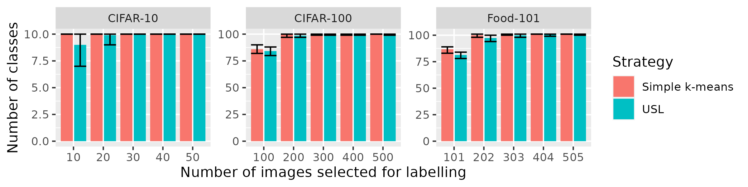
(a) Average number of classes sampled over 20 runs. Error bars show maximum and minimum number of classes sampled.

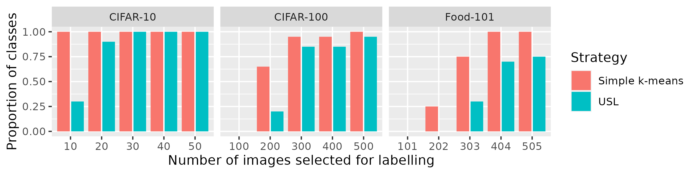
(b) Proportion of sets sampling all classes over 20 runs.

Figure 3: Comparison of USL and simple $k$-means prototype selection using classes from several datasets. We compare how well USL and simple $k$-means prototype selection fares on the challenge of selecting as many classes within a dataset as possible for a small labelling budget. The latter approach outperforms USL on these three datasets, consistently sampling more diverse sets of prototypes in each case.

When using prototype selection strategies, it can be the case that for small budgets some classes are not sampled. This can cause issues with the sets of hyperparameters being chosen for a particular method no longer being valid. This is the case for the PAWS class stratified sampler, which selects prototypes from a select number of classes. While modifications could have been made to allow the models to fit with a reduced set of classes, this reduces the maximum attainable performance for a model as unsampled classes cannot be learned within the PAWS framework. We did not fit models in cases where the hyperparameters became invalid, such as for the USL method where less than 100 classes were sampled for the Food-101 dataset.

We compare the ability of USL and the simple $k$-means approach to sample all of the classes present in a dataset in Fig. 3. We find that in the three cases we considered, the simple $k$-means strategy samples a greater diversity of images, as measured by the number of classes sampled from each dataset for a given budget.

References

- Assran et al. [2021] Mahmoud Assran, Mathilde Caron, Ishan Misra, Piotr Bojanowski, Armand Joulin, Nicolas Ballas, and Michael Rabbat. Semi-supervised learning of visual features by non-parametrically predicting view assignments with support samples. In Proceedings of the IEEE/CVF International Conference on Computer Vision, pages 8443–8452, 2021.
- Bao et al. [2021] Hangbo Bao, Li Dong, Songhao Piao, and Furu Wei. Beit: Bert pre-training of image transformers. arXiv preprint arXiv:2106.08254, 2021.
- Berthelot et al. [2019] David Berthelot, Nicholas Carlini, Ian Goodfellow, Nicolas Papernot, Avital Oliver, and Colin A Raffel. Mixmatch: A holistic approach to semi-supervised learning. Advances in neural information processing systems, 32, 2019.
- Bossard et al. [2014] Lukas Bossard, Matthieu Guillaumin, and Luc Van Gool. Food-101–mining discriminative components with random forests. In Computer Vision–ECCV 2014: 13th European Conference, Zurich, Switzerland, September 6-12, 2014, Proceedings, Part VI 13, pages 446–461. Springer, 2014.
- Cai et al. [2022] Zhaowei Cai, Avinash Ravichandran, Paolo Favaro, Manchen Wang, Davide Modolo, Rahul Bhotika, Zhuowen Tu, and Stefano Soatto. Semi-supervised vision transformers at scale. Advances in Neural Information Processing Systems, 35:25697–25710, 2022.
- Carlini et al. [2019] Nicholas Carlini, Ulfar Erlingsson, and Nicolas Papernot. Distribution density, tails, and outliers in machine learning: Metrics and applications. arXiv preprint arXiv:1910.13427, 2019.
- Caron et al. [2020] Mathilde Caron, Ishan Misra, Julien Mairal, Priya Goyal, Piotr Bojanowski, and Armand Joulin. Unsupervised learning of visual features by contrasting cluster assignments. Advances in neural information processing systems, 33:9912–9924, 2020.
- Caron et al. [2021] Mathilde Caron, Hugo Touvron, Ishan Misra, Hervé Jégou, Julien Mairal, Piotr Bojanowski, and Armand Joulin. Emerging properties in self-supervised vision transformers. In Proceedings of the IEEE/CVF international conference on computer vision, pages 9650–9660, 2021.
- Chen et al. [2022] Liangyu Chen, Yutong Bai, Siyu Huang, Yongyi Lu, Bihan Wen, Alan L Yuille, and Zongwei Zhou. Making your first choice: To address cold start problem in vision active learning. arXiv preprint arXiv:2210.02442, 2022.
- Chen et al. [2020a] Ting Chen, Simon Kornblith, Mohammad Norouzi, and Geoffrey Hinton. A simple framework for contrastive learning of visual representations. In International conference on machine learning, pages 1597–1607. PMLR, 2020a.
- Chen et al. [2020b] Ting Chen, Simon Kornblith, Kevin Swersky, Mohammad Norouzi, and Geoffrey E Hinton. Big self-supervised models are strong semi-supervised learners. Advances in neural information processing systems, 33:22243–22255, 2020b.
- Falcon and The PyTorch Lightning team [2019] William Falcon and The PyTorch Lightning team. PyTorch Lightning, 2019.
- Fostiropoulos and Itti [2022] Iordanis Fostiropoulos and Laurent Itti. Supervised contrastive prototype learning: Augmentation free robust neural network. arXiv preprint arXiv:2211.14424, 2022.
- Govindarajan et al. [2022] Hariprasath Govindarajan, Per Sidén, Jacob Roll, and Fredrik Lindsten. Dino as a von mises-fisher mixture model. In The Eleventh International Conference on Learning Representations, 2022.
- Grill et al. [2020] Jean-Bastien Grill, Florian Strub, Florent Altché, Corentin Tallec, Pierre Richemond, Elena Buchatskaya, Carl Doersch, Bernardo Avila Pires, Zhaohan Guo, Mohammad Gheshlaghi Azar, et al. Bootstrap your own latent-a new approach to self-supervised learning. Advances in neural information processing systems, 33:21271–21284, 2020.
- Helber et al. [2019] Patrick Helber, Benjamin Bischke, Andreas Dengel, and Damian Borth. Eurosat: A novel dataset and deep learning benchmark for land use and land cover classification. IEEE Journal of Selected Topics in Applied Earth Observations and Remote Sensing, 12(7):2217–2226, 2019.
- Hinton et al. [2015] Geoffrey Hinton, Oriol Vinyals, and Jeff Dean. Distilling the knowledge in a neural network. arXiv preprint arXiv:1503.02531, 2015.
- Hinton and Roweis [2002] Geoffrey E Hinton and Sam Roweis. Stochastic neighbor embedding. Advances in neural information processing systems, 15, 2002.
- Kobak and Berens [2019] Dmitry Kobak and Philipp Berens. The art of using t-sne for single-cell transcriptomics. Nature communications, 10(1):5416, 2019.
- Krizhevsky et al. [2009] Alex Krizhevsky, Geoffrey Hinton, et al. Learning multiple layers of features from tiny images. 2009.
- Lloyd [1982] Stuart Lloyd. Least squares quantization in pcm. IEEE transactions on information theory, 28(2):129–137, 1982.
- Ming et al. [2022] Yifei Ming, Yiyou Sun, Ousmane Dia, and Yixuan Li. How to exploit hyperspherical embeddings for out-of-distribution detection? arXiv preprint arXiv:2203.04450, 2022.
- Mo et al. [2023] Sangwoo Mo, Jong-Chyi Su, Chih-Yao Ma, Mido Assran, Ishan Misra, Licheng Yu, and Sean Bell. Ropaws: Robust semi-supervised representation learning from uncurated data. arXiv preprint arXiv:2302.14483, 2023.
- Nilsback and Zisserman [2008] Maria-Elena Nilsback and Andrew Zisserman. Automated flower classification over a large number of classes. In 2008 Sixth Indian conference on computer vision, graphics & image processing, pages 722–729. IEEE, 2008.
- Olsen et al. [2019] Alex Olsen, Dmitry A Konovalov, Bronson Philippa, Peter Ridd, Jake C Wood, Jamie Johns, Wesley Banks, Benjamin Girgenti, Owen Kenny, James Whinney, et al. Deepweeds: A multiclass weed species image dataset for deep learning. Scientific reports, 9(1):2058, 2019.
- Oquab et al. [2023] Maxime Oquab, Timothée Darcet, Théo Moutakanni, Huy Vo, Marc Szafraniec, Vasil Khalidov, Pierre Fernandez, Daniel Haziza, Francisco Massa, Alaaeldin El-Nouby, et al. Dinov2: Learning robust visual features without supervision. arXiv preprint arXiv:2304.07193, 2023.
- Parkhi et al. [2012] Omkar M Parkhi, Andrea Vedaldi, Andrew Zisserman, and CV Jawahar. Cats and dogs. In 2012 IEEE conference on computer vision and pattern recognition, pages 3498–3505. IEEE, 2012.
- Paszke et al. [2019] Adam Paszke, Sam Gross, Francisco Massa, Adam Lerer, James Bradbury, Gregory Chanan, Trevor Killeen, Zeming Lin, Natalia Gimelshein, Luca Antiga, Alban Desmaison, Andreas Kopf, Edward Yang, Zachary DeVito, Martin Raison, Alykhan Tejani, Sasank Chilamkurthy, Benoit Steiner, Lu Fang, Junjie Bai, and Soumith Chintala. PyTorch: An Imperative Style, High-Performance Deep Learning Library. In Advances in Neural Information Processing Systems 32, pages 8024–8035. Curran Associates, Inc., 2019.
- Radford et al. [2021] Alec Radford, Jong Wook Kim, Chris Hallacy, Aditya Ramesh, Gabriel Goh, Sandhini Agarwal, Girish Sastry, Amanda Askell, Pamela Mishkin, Jack Clark, et al. Learning transferable visual models from natural language supervision. In International conference on machine learning, pages 8748–8763. PMLR, 2021.
- Rani et al. [2023] Veenu Rani, Syed Tufael Nabi, Munish Kumar, Ajay Mittal, and Krishan Kumar. Self-supervised learning: A succinct review. Archives of Computational Methods in Engineering, 30(4):2761–2775, 2023.
- Raschka et al. [2020] Sebastian Raschka, Joshua Patterson, and Corey Nolet. Machine learning in python: Main developments and technology trends in data science, machine learning, and artificial intelligence. arXiv preprint arXiv:2002.04803, 2020.
- Rossi and Barbaro [2022] Fabrice Rossi and Florian Barbaro. Mixture of von mises-fisher distribution with sparse prototypes. Neurocomputing, 501:41–74, 2022.
- Rule and Riesenhuber [2021] Joshua S Rule and Maximilian Riesenhuber. Leveraging prior concept learning improves generalization from few examples in computational models of human object recognition. Frontiers in Computational Neuroscience, 14:117, 2021.
- Shu et al. [2018] Rui Shu, Hung H Bui, Shengjia Zhao, Mykel J Kochenderfer, and Stefano Ermon. Amortized inference regularization. Advances in Neural Information Processing Systems, 31, 2018.
- Sohn et al. [2020] Kihyuk Sohn, David Berthelot, Nicholas Carlini, Zizhao Zhang, Han Zhang, Colin A Raffel, Ekin Dogus Cubuk, Alexey Kurakin, and Chun-Liang Li. Fixmatch: Simplifying semi-supervised learning with consistency and confidence. Advances in neural information processing systems, 33:596–608, 2020.
- Van Der Maaten [2009] Laurens Van Der Maaten. Learning a parametric embedding by preserving local structure. In Artificial intelligence and statistics, pages 384–391. PMLR, 2009.
- Van der Maaten and Hinton [2008] Laurens Van der Maaten and Geoffrey Hinton. Visualizing data using t-sne. Journal of machine learning research, 9(11), 2008.
- Van Engelen and Hoos [2020] Jesper E Van Engelen and Holger H Hoos. A survey on semi-supervised learning. Machine learning, 109(2):373–440, 2020.
- Wang and Wang [2016] Mian Wang and Dong Wang. Vmf-sne: Embedding for spherical data. In 2016 IEEE International Conference on Acoustics, Speech and Signal Processing (ICASSP), pages 2344–2348. IEEE, 2016.
- Wang et al. [2022a] Xudong Wang, Long Lian, and Stella X Yu. Unsupervised selective labeling for more effective semi-supervised learning. In European Conference on Computer Vision, pages 427–445. Springer, 2022a.
- Wang et al. [2021] Yingfan Wang, Haiyang Huang, Cynthia Rudin, and Yaron Shaposhnik. Understanding how dimension reduction tools work: an empirical approach to deciphering t-sne, umap, trimap, and pacmap for data visualization. The Journal of Machine Learning Research, 22(1):9129–9201, 2021.
- Wang et al. [2022b] Yidong Wang, Hao Chen, Qiang Heng, Wenxin Hou, Yue Fan, Zhen Wu, Jindong Wang, Marios Savvides, Takahiro Shinozaki, Bhiksha Raj, et al. Freematch: Self-adaptive thresholding for semi-supervised learning. In The Eleventh International Conference on Learning Representations, 2022b.
- Wu et al. [2018] Zhirong Wu, Yuanjun Xiong, Stella X Yu, and Dahua Lin. Unsupervised feature learning via non-parametric instance discrimination. In Proceedings of the IEEE conference on computer vision and pattern recognition, pages 3733–3742, 2018.
- Yadan [2019] Omry Yadan. Hydra - a framework for elegantly configuring complex applications. Github, 2019.
- Yang et al. [2018] Hong-Ming Yang, Xu-Yao Zhang, Fei Yin, and Cheng-Lin Liu. Robust classification with convolutional prototype learning. In Proceedings of the IEEE conference on computer vision and pattern recognition, pages 3474–3482, 2018.
- Yang et al. [2023] Lihe Yang, Zhen Zhao, Lei Qi, Yu Qiao, Yinghuan Shi, and Hengshuang Zhao. Shrinking class space for enhanced certainty in semi-supervised learning. In Proceedings of the IEEE/CVF International Conference on Computer Vision, pages 16187–16196, 2023.
- You et al. [2017] Yang You, Igor Gitman, and Boris Ginsburg. Large batch training of convolutional networks. arXiv preprint arXiv:1708.03888, 2017.
- Zhou et al. [2023] Ce Zhou, Qian Li, Chen Li, Jun Yu, Yixin Liu, Guangjing Wang, Kai Zhang, Cheng Ji, Qiben Yan, Lifang He, et al. A comprehensive survey on pretrained foundation models: A history from bert to chatgpt. arXiv preprint arXiv:2302.09419, 2023.
- Zhou et al. [2021] Jinghao Zhou, Chen Wei, Huiyu Wang, Wei Shen, Cihang Xie, Alan Yuille, and Tao Kong. ibot: Image bert pre-training with online tokenizer. arXiv preprint arXiv:2111.07832, 2021.