Beyond Sole Strength:
Customized Ensembles for Generalized Vision-Language Models

Abstract

Fine-tuning pre-trained vision-language models (VLMs), e.g., CLIP, for the open-world generalization has gained increasing popularity due to its practical value. However, performance advancements are limited when relying solely on intricate algorithmic designs for a single model, even one exhibiting strong performance, e.g., CLIP-ViT-B/16. This paper, for the first time, explores the collaborative potential of leveraging much weaker VLMs to enhance the generalization of a robust single model. The affirmative findings motivate us to address the generalization problem from a novel perspective, i.e., ensemble of pre-trained VLMs. We introduce three customized ensemble strategies, each tailored to one specific scenario. Firstly, we introduce the zero-shot ensemble, automatically adjusting the logits of different models based on their confidence when only pre-trained VLMs are available. Furthermore, for scenarios with extra few-shot samples, we propose the training-free and tuning ensemble, offering flexibility based on the availability of computing resources. The proposed ensemble strategies are evaluated on zero-shot, base-to-new, and cross-dataset generalization, achieving new state-of-the-art performance. Notably, this work represents an initial stride toward enhancing the generalization performance of VLMs via ensemble. The code is available at https://github.com/zhiheLu/Ensemble_VLM.git.

1 Introduction

Pre-trained large-scale vision-language models (VLMs), e.g., CLIP [51] and ALIGN [29], have demonstrated remarkable recognition performance on open-vocabulary downstream tasks even in a zero-shot evaluation manner. This advancement overcomes the constraint observed in prior supervised deep models [26], which are limited to classify seen classes only, i.e., test set should share the same label space with the training set. Encouraged by the impressive zero-shot generalization of VLMs, recent works [73, 72, 68, 40, 21, 70] have explored how to adapt the VLMs for better performance on downstream tasks in an efficient tuning fashion, where only few-shot samples and limited learnable parameters are used.

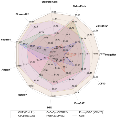
Figure 1: Comparing existing methods on base-to-new generalization. The results indicate that the proposed method outperforms existing arts on 11 diverse datasets, often by large margins.

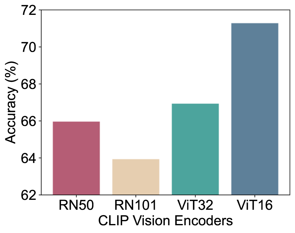
(a) Flowers102

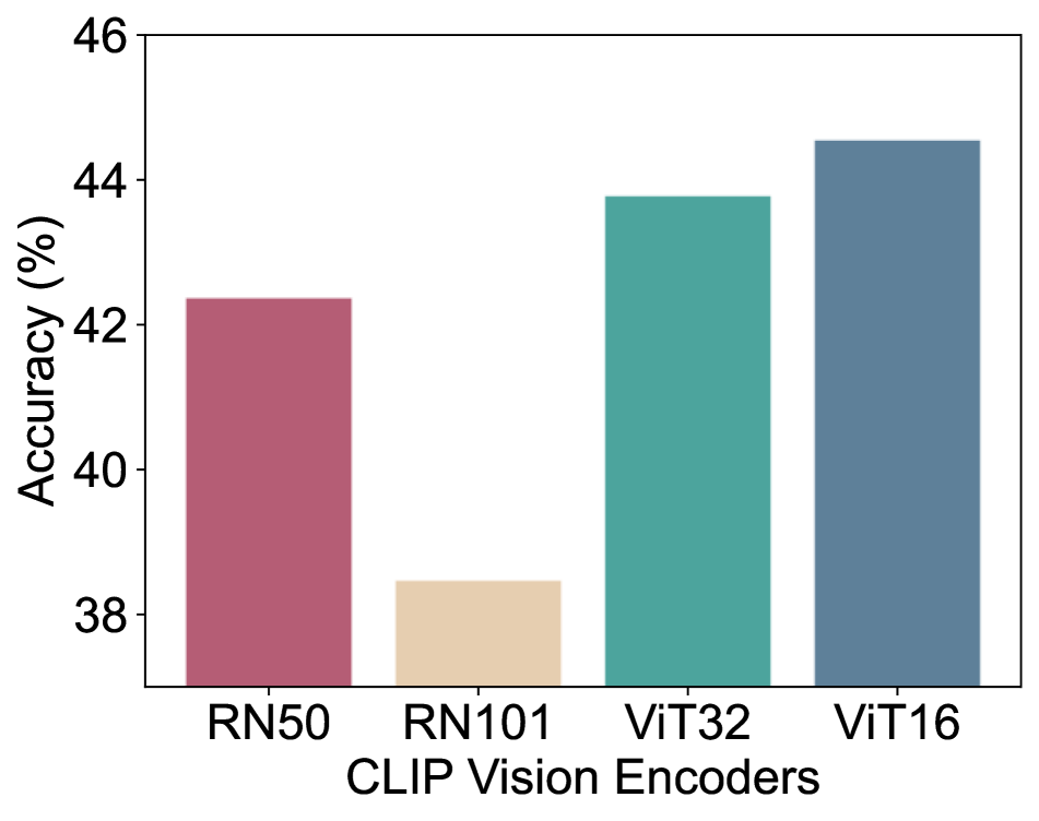
(b) DTD

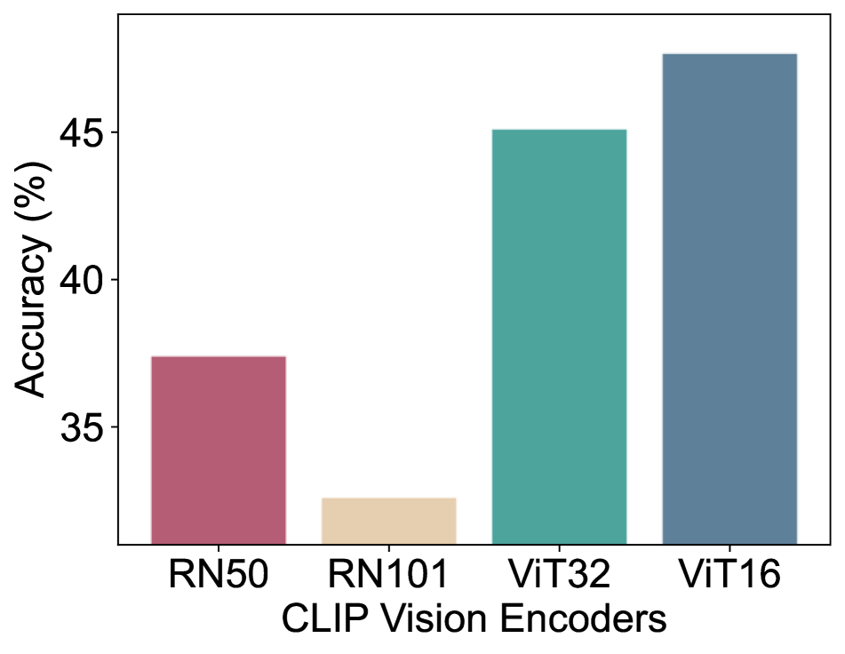
(c) EuroSAT

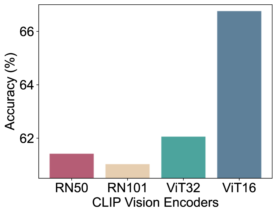
(d) UCF101

Figure 2: Zero-shot evaluation of pre-trained CLIP vision encoders on varying datasets. The bar charts show that the “seemingly weakest” model RN50 may perform better than RN101 in some cases, encouraging us to leverage diverse models for enhanced ensemble.

For the efficient adaptation of VLMs, prompt learning [73] is a popular solution. The concept of prompt learning was first proposed in natural language processing (NLP) [54, 30, 71], which is to learn a prompt that dynamically suits the downstream tasks instead of prompt engineering. CoOp [73] was the first work to introduce prompt learning for adapting VLMs and it outperforms both handcrafted prompts and the linear probe model. However, a critical problem of CoOp is that the learned prompt on base classes performs poorly when applied to unseen new classes even under the same data distribution. CoCoOp [72] hence has been proposed to improve the performance of this base-to-new set-up by conditioning the prompt learning with the image context. To further advance the base-to-new generalization, recent works have been proposed to leverage multi-modal prompt learning (MaPLe) [34], self-regulating constraints (PromptSRC) [35], or synthesized prompts (SHIP) [63]. It is worth noting that the default CLIP model used in these methods is ViT-B/16 [14], one of the strongest CLIP models in Transformer structure [61]. However, their performance on new classes is still not satisfactory, e.g., 70.43% (CoCoOp, CVPR22) $\rightarrow$ 70.54% (MaPLe, CVPR23) $\rightarrow$ 70.26% (SHIP, ICCV23) $\rightarrow$ 70.73% (PromptSRC, ICCV23) on ImageNet. One possible reason is that with the advanced algorithms, the knowledge of a single model has already been fully explored for generalization, thereby leading to limited improvement. As such, one question naturally arises: can we leverage the prior knowledge from multiple CLIP models for better generalization even though some of them are weaker performers?

To this end, we first investigate the zero-shot performance of four widely used CLIP models, i.e., RN50, RN101, ViT-B/32 and ViT-B/16, on 11 diverse datasets as shown in Table 1. Intuitively, a larger model should yield better performance, but we have observed that this is not always the case across all datasets. For instance, the “weakest” model RN50 outperforms RN101 on four datasets (refer to Figure 2). This indicates that models with distinct architectures are inclined to predict different samples correctly, as those models may develop biases even when trained on the same dataset. We posit that these model biases can be leveraged for improved generalization in open-world scenarios. Indeed, zero-shot experiments (see Table 2) demonstrate enhanced generalization by combining any weaker CLIP model with CLIP-ViT-B/16 while using all models performs the best.

Inspired by the favorable results of a simple ensemble, we further design three types of ensemble strategies, each tailored for a practical scenario. First, given solely CLIP models, we introduce the zero-shot ensemble (ZS_En), which employs confidence-aware weighting for the weaker models while preserving the dominance of the strongest model. This confidence-aware weighting dynamically adjusts the weights of the models’ logits based on their prediction confidences of input samples. Second, in scenarios where additional few-shot samples ($D_{train}$) are available but without training resources, we propose the training-free ensemble (TF_En). This ensemble method leverages a greedy search to determine the “optimal” weights for model ensemble, identified when the accuracy of the ensemble is maximized on $D_{train}$. Third, when pre-trained models, $D_{train}$ and training resources exist simultaneously, the tuning ensemble (T_En) is proposed by learning a sample-aware weight generator (SWIG). Specifically, the proposed SWIG takes the visual features of multiple models as input and automatically generates the ensemble weights through optimizing on the training data.

To assess the proposed methods, we employ ZS_En for zero-shot generalization, TF_En and T_En for base-to-new generalization on 11 diverse datasets. Additionally, we examine the effectiveness of T_En on cross-dataset evaluation. On all tasks, our methods always yield new state-of-the-art performance, often surpassing the second best by large margins (e.g., see the results of base-to-new generalization in Figure 1). More importantly, this work offers a new possibility for the enhanced generalization of VLMs by overcoming the limitation of existing works that rely solely on designing intricate algorithms for a single VLM.

We summarize our contributions as follows:

• Having observed the saturated generalization performance achieved by fully exploring the knowledge from a single robust VLM, we, for the first time, propose to advance the generalization through ensemble learning.

• We propose three ensemble strategies, each tailored for a practical situation. First, in cases where only CLIP models are available, we introduce the confidence-aware weighting based zero-shot ensemble (ZS_En). Second, when additional few-shot samples ($D_{train}$) are accessible but without extra training resources, we present the training-free ensemble based on greedy search (TF_En). Third, in scenarios where pre-trained models, $D_{train}$, and training resources coexist, we propose the tuning ensemble (T_En) by incorporating a sample-aware weight generator (SWIG).

• We assess ZS_En for zero-shot generalization, achieving an average accuracy gain of 2.61% across 11 diverse datasets. Additionally, we evaluate T_En for base-to-new and cross-dataset generalization, yielding new state-of-the-art performance.

• Moreover, this work establishes a pathway for improved generalization in VLMs, surpassing the limitations of prior methods that depend solely on crafting intricate algorithms for a single VLM.

2 Related Work

2.1 Vision-Language Models

Vision-language models (VLMs) have obtained huge popularity due to its many potential applications, such as visual question answering [23, 24, 45, 55], visual captioning [1, 42, 20], visual language reasoning [31, 58, 69], language driven visual generation [52, 48], language driven visual representation learning (LDVRL) [56, 19, 15, 38, 32, 22, 39, 12, 53, 51, 1], et al. We mainly focus on LDVRL in this paper. LDVRL based VLMs often adopt two encoders for language and vision, respectively, and are optimized by tailored matching constraints [56, 22].

Chronologically, early works employ varied approaches for language and vision modeling. For language, they utilize methods like unsupervised pre-trained models [56] or skip-gram text modeling [19, 46, 47]. Meanwhile, for vision, these works explore techniques like sparse coding and vector quantization [56, 8] or utilize features such as Classeme [15, 59]. In recent works [51, 29, 41], a common trend is the utilization of two deep neural networks, e.g., Transformers [61, 13, 60], to independently embed language and vision inputs. These works generally pre-train on million/billion-level image-text pairs from internet, e.g., $\sim$400M for CLIP [51] and $\sim$1B for ALIGN [29], employing a contrastive loss. The resulting pre-trained VLMs showcase impressive zero-shot generalization across a range of downstream tasks. In this paper, we endeavor to improve their zero-shot generalization by effectively leveraging the knowledge embedded in multiple models.

2.2 Zero-Shot Generalization of VLMs

Zero-shot generalization/learning (ZSG) [6, 62, 65, 67] aims to recognize novel classes by training only on base classes. Past ZSG works often learn the compositions of attributes [28] and word embeddings [19, 30] on base classes to tackle “seen-class bias” issue. The advent of large-scale VLMs introduces novel possibilities for addressing ZSG. These VLMs, trained to align image-and-text pairs, can be employed for ZSG on novel classes simply by adopting prompts of those novel classes for the language encoder.

To further advance the performance of ZSG on downstream tasks, prompt learning [73, 72] has been proposed to learn a prompt on base classes that exhibits better generalization on novel classes within the same data distribution. MaPLe [34] explores multi-model prompt learning by jointly learning hierarchical prompts at two branches of CLIP, aiming for improved generalization performance. Recent works have introduced approaches leveraging self-regulating constraints [35] and synthesized prompts [63]. Despite the intricate algorithms designed, the performance improvement on ZSG remains limited. One potential reason is that the knowledge stored in a single model has been thoroughly explored, making further improvement challenging. To that end, we take the initial step in exploring knowledge from multiple VLMs to enhance generalization.

2.3 Ensemble Learning

Ensemble learning (EL) [3, 4, 5, 25, 17, 18, 9, 64, 37, 11, 33] is a machine learning paradigm where multiple models, often of diverse types, are combined to improve overall predictive performance and generalization. Technically, EL methods can be broadly categorized into three main types: Bagging (Bootstrap Aggregating) [3, 4, 5, 25], Boosting [17, 18, 9] and Stacking [64, 37, 11, 33]. Bagging was initially proposed in 1996 by Breiman [3]. The technique involves training multiple models of the same structure on diverse subsets obtained through bootstrap sampling. Boosting [17, 18, 9] is employed in ensemble models to transform several weak learners into one with improved generalization. In contrast, Stacking [64, 37, 11, 33] is an integration technique where a meta-learning model is used to combine the outputs of base models. In this paper, we resort to ensemble learning for better generalization of VLMs, with a specific emphasis on prediction fusion strategies in both training-free and tuning fashions.

3 Methodology

In this section, we first briefly introduce Vision-Language Model (VLM) employed in our method, namely CLIP [51]. Subsequently, we present three specific ensemble strategies designed to leverage VLMs for enhanced generalization in downstream tasks. The VLMs employed in this work are four widely used CLIP models: CLIP-RN50, CLIP-RN101, CLIP-ViT-B/32, and CLIP-ViT-B/16. Note that the backbones here mainly refer to the vision encoder.

3.1 Preliminaries

The CLIP [51] model is pre-trained on $\sim$400M image-text pairs with the objective of aligning two modalities within a unified embedding space using a contrastive learning loss. This pre-training enables CLIP to effectively capture broad visual concepts and learn general visual representations. During inference, a given image can be classified into a pre-defined category by computing the similarity between the image feature $\mathbf{f}$ extracted from the vision encoder and the textual embeddings $\{\mathbf{c}_{i}|i\in\{1,\dots,K\}\}$ from the language encoder. The inputs to the language encoder are textual prompts for $K$ categories, composed of a template, e.g., “a photo of a $\{class\}$”, and category names. This classification approach allows CLIP to be directly applied to a new recognition task with only the category names of interest. We formulate the inference process as follows:

$$\mathbf{Logit}_{i}=\frac{exp(cos(\mathbf{f},\mathbf{c}_{i})/\tau)}{\sum_{j=1}^{K}exp(cos(\mathbf{f},\mathbf{c}_{i})/\tau)}$$ (1)

, where $cos(\cdot,\cdot)$ is the cosine similarity function and $\tau$ is the learned temperature parameter.

3.2 Zero-shot Ensemble

The proposed zero-shot ensemble (ZS_En) aims to enhance the generalization capability of VLMs using solely pre-trained CLIP models as shown in Figure 3. Specifically, our ensemble strategy is designed with two key perspectives: (i) maintaining the dominance of the best-performing model, i.e., CLIP-ViT-B/16; (ii) dynamically assigning weights to individual models based on their confidence for the given samples. The first consideration is grounded in the fact that CLIP-ViT-B/16, with inputting large patches and advanced Transformer architecture, can capture superior visual representations, leading to heightened transferability on downstream tasks. This is evidenced by the substantial zero-shot performance gaps observed between CLIP-ViT-B/16 and other variants. Consequently, preserving the dominance of CLIP-ViT-B/16 is deemed essential. To automate the weight generation for model ensemble, we propose to use confidence-aware weights by dynamically adjusting the contribution of individual models’ logits based on their prediction confidences on input samples. The formulation of above process is defined as

$$\mathbf{p}_{i} =max(\mathbf{Logit}_{i}:\{p_{1},p_{2},\dots,p_{K}\})$$ (2)

$$\mathbf{\omega}_{i} =\frac{exp(\mathbf{p}_{i})}{\sum_{j=1}^{n-1}exp(\mathbf{p}_{j})}$$ (3)

$$\mathbf{Logit}_{e} =\sum_{i=1}^{n-1}\mathbf{\omega}_{i}\cdot\mathbf{Logit}_{i}+\mathbf{Logit}_{n}$$ (4)

, where $\mathbf{p}_{i}$ is the maximum prob of $\mathbf{Logit}_{i}$, $\mathbf{Logit}_{i}$ is the logit from the $i$-th VLM for an input image, $\mathbf{Logit}_{n}$ is the strongest VLM of n ensemble VLMs. It is worth noting that our ZS_En enhances the overall generalization capability of VLMs without the need for additional training data or computing resources.

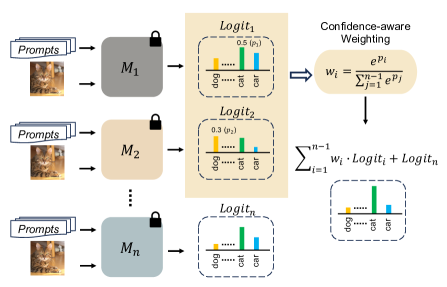
Figure 3: Illustration of our zero-shot ensemble (ZS_En). We assign a weight 1.0 to the best performing model, i.e., CLIP-ViT-B/16, and use the confidence-aware weights for other VLMs.

3.3 Training-free Ensemble

We propose a training-free ensemble (see Figure 4) to further enhance the generalization of VLMs in scenarios where additional few-shot samples $D_{train}$ are available but there are constraints on computing resources for training. Note that the classes in $D_{train}$ are disjoint from those in $D_{test}$ during inference, rendering this set-up both more challenging and practical. Specifically, we implement the training-free ensemble by employing greedy search to find the optimal accuracy on a training set. The desired weights $\{\omega_{i}\}$ are then determined when the optimal accuracy is achieved. The rationale behind this approach is that samples within the same data distribution can be utilized to search for optimal parameters for classifying new classes, aligning with methodologies for base-to-new generalization [72, 34, 35]. To be specific, we formulate the above process as follows:

$$\{\omega_{i}\} =\mathop{argmax}_{\{\omega_{i}\}}(\frac{1}{N}\sum_{j=1}^{N}\delta(y_{i},\hat{y}_{i})|D_{train})$$ (5)

$$\hat{y}_{i} =argmax(\sum_{j=1}^{n-1}\omega_{i}\cdot\mathbf{Logit}_{i}+\mathbf{Logit}_{n})$$ (6)

, where $N$ is the total number of samples in $D_{train}$, $y_{i}$ is the true label of the $i$-th sample, $\hat{y}_{i}$ is the predicted label of the $i$-th sample, $\delta(\cdot,\cdot)$ is the Kronecker delta function, which is equal to 1 if $y_{i}=\hat{y}_{i}$ and 0 otherwise.

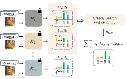
Figure 4: Illustration of our training-free ensemble (TF_En). We assign a weight 1.0 to the best performing model, i.e., CLIP-ViT-B/16, and determine the weights of other VLMs by greedy searching on a given “training” set without training.

3.4 Tuning Ensemble

Following the set-up of previous works [72, 34, 35], we introduce the tuning ensemble as illustrated in Figure 5. This ensemble method employs a meta-model, sample-aware weight generator (SWIG), to learn the generation of weights on the training set $D_{train}$. The advantage of the tuning ensemble, in comparison to the training-free version, lies in our SWIG’s capability to dynamically generate weights for each sample based on the features of ensemble models. This facilitates test-sample-aware weight generation, with the corresponding features serving as inputs.

Concretely, to implement this tuning ensemble, we initially obtain the features $\{I_{f}^{1},\dots,I_{f}^{n}\}$ of the input image by passing it through the vision encoders of the employed VLMs. Subsequently, these features are concatenated and used as the input to our proposed SWIG, which generates weights $\{\omega_{1},\dots,\omega_{n}\}$ for the ensemble of VLMs. These dynamically generated weights serve as a form of sample-specific attention, allowing the ensemble to adapt to the characteristics of each input image. This personalized weight assignment enhances the tuning ensemble’s ability to tailor its predictions based on the unique features of the test samples, thereby contributing to improved generalization performance. The aforementioned process can be formulated with the following equations:

$$I_{f}^{1},I_{f}^{2},\dots,I_{f}^{n} =E_{I}^{1}(x),E_{I}^{2}(x),\dots,E_{I}^{n}(x)$$ (7)

$$\{\omega_{1},\dots,\omega_{n}\} =\Theta_{SWIG}(concat(\{I_{f}^{1},\dots,I_{f}^{n}\}))$$ (8)

$$\mathbf{Logit}_{e} =\sum_{i=1}^{n}\mathbf{\omega}_{i}\cdot\mathbf{Logit}_{i}$$ (9)

, where $E_{I}^{i}$ is the vision encoder of the $i$-th VLM, $x$ is the input image and $\Theta_{SWIG}$ is our sample-aware weight generator.

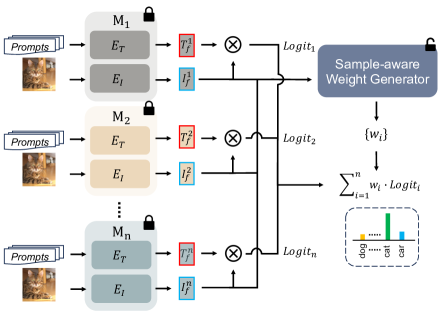
Figure 5: Illustration of our tuning ensemble (T_En). The proposed sample-aware weight generator (SWIG) takes sample features as input to generate sample-aware weights, which are then used for weighted prediction.

Remark

The choice of using image features, rather than logits, as the input to our SWIG is motivated by the unique prediction mechanism of VLMs. VLMs calculate the cosine similarity between the image feature and textual embeddings to generate logits. If logits were used as the input for SWIG, the generated weights might be biased towards the textual embeddings of base classes. This bias is undesirable for generalization to novel classes. By utilizing image features as the input for SWIG, we can effectively avoid this drawback. This approach ensures that SWIG remains sample-aware and generalizes well.

4 Experiments

In this section, we orderly introduce the datasets and metrics used, implementation details, and evaluation on zero-shot, base-to-new and cross-dataset generalization.

4.1 Datasets and Metrics

In general, we assess the effectiveness of the three proposed ensemble strategies across three generalization scenarios: (i) zero-shot; (ii) base-to-new; and (iii) cross-dataset. All experiments are conducted on 11 diverse datasets, and the quantitative evaluation metric is classification accuracy.

Datasets

Following prior research [73, 72, 34, 35], we employ a set of 11 diverse datasets, covering a range of recognition tasks. Specifically, the benchmark comprises the following datasets: (i) ImageNet [10] and Caltech101 [16] for generic object classification; (ii) OxfordPets [50], StanfordCars [36], Flowers102 [49], Food101 [2], and FGVCAircraft [44] for fine-grained classification; (iii) SUN397 [66] for scene recognition; (iv) UCF101 [57] for action recognition; (v) DTD [7] for texture classification; (vi) EuroSAT [27] for satellite imagery recognition.

Evaluation Metrics

For zero-shot generalization, only the original test set of each dataset is used for computing accuracy since no training is needed. In the base-to-new generalization setup, we follow [73, 72, 34, 35] to equally split the classes into two groups, i.e., base and new classes, and then randomly sample a 16-shot training set from base classes. The learned model is then evaluated on both base and new classes from test set. We report three accuracy metrics: accuracy on base classes, accuracy on new classes and the harmonic mean (HM) of these two accuracies. In contrast, for cross-dataset generalization, a model is trained on ImageNet [10] and then conducted cross-validation on the remaining datasets. Note that the presented results are averaged over three runs, except for zero-shot generalization.

4.2 Implementation Details

In our experiments, we utilize four widely used CLIP models for ensemble learning: CLIP-RN50, CLIP-RN101, CLIP-ViT-B/32, and CLIP-ViT-B/16, with CLIP-ViT-B/16 being the best performer. In all three ensemble strategies, the $\mathbf{Logit}$ is computed by applying the softmax function to a model’s prediction. For the training-free ensemble, the weight search space is fixed at $\{0.1,0.2,\dots,1.0\}$ for each VLM, excluding CLIP-ViT-B/16. For the tuning ensemble, we set the initial learning rate to $5e-3$ and utilize the same adjusting scheduler as in [72, 34, 35]. The sample-aware weight generator is a two-layer MLP ($f_{dim}\rightarrow f_{dim}/32$ and $f_{dim}/32\rightarrow num_{weight}$), which is trained for 5 epochs with a batch size of 128. The tuning ensemble is applied to both pre-trained CLIP models and existing baseline methods.

Dataset	CLIP	CLIP	CLIP	CLIP	ZSEn	$\Delta$
	RN50	RN101	ViT-B/32	ViT-B/16	Ours
Average	58.71	59.52	61.87	65.27	67.88	+2.61
ImageNet	58.23	61.26	62.04	66.72	70.66	+3.94
Caltech101	85.96	89.66	91.12	92.94	93.79	+0.85
OxfordPets	85.80	86.89	87.49	89.07	90.57	+1.50
Stanford Cars	55.57	63.16	60.37	65.29	70.76	+5.47
Flowers102	65.98	63.95	66.95	71.30	73.16	+1.86
Food101	77.32	80.54	80.47	86.11	86.78	+0.67
FGVC Aircraft	17.16	18.18	19.20	24.87	25.68	+0.81
SUN397	58.53	58.96	62.00	62.62	65.91	+3.29
DTD	42.38	38.48	43.79	44.56	49.35	+4.79
EuroSAT	37.42	32.62	45.12	47.69	50.20	+2.51
UCF101	61.43	61.04	62.07	66.77	69.84	+3.07

Table 1: Zero-shot generalization. All compared methods are implemneted on the pre-trained CLIP [51] models without further training. Absolute gains over baseline are shown in blue.

CLIP	CLIP	CLIP	CLIP	Acc	$\Delta$
ViT-B/16	RN50	RN101	ViT-B/32
$\checkmark$				66.72	+0.00
$\checkmark$	$\checkmark$			67.75	+1.03
$\checkmark$	$\checkmark$	$\checkmark$		68.34	+1.62
$\checkmark$	$\checkmark$	$\checkmark$	$\checkmark$	68.76	+2.04

Table 2: The ensemble of the CLIP-ViT-B/16 model with other weaker variants on ImageNet.

Method	Acc	$\Delta$
CLIP ViT-B/16	66.72	+0.00
Baseline	68.76	+2.04
CAW of 3 models (w/o RN50)	70.01	+3.29
CAW of 4 models	70.19	+3.47
CLIP ViT-B/16 + CAW of 3 other models	70.66	+3.94

Table 3: Evaluating confidence-aware weighting (CAW) in different manners on ImageNet. Baseline uses the mean of the logits from four models as the final prediction.

	Average			ImageNet [10]			Caltech101 [16]			OxfordPets [50]
	Base	New	HM	Base	New	HM	Base	New	HM	Base	New	HM
CLIP [51]	69.34	74.22	71.70	72.43	68.14	70.22	96.84	94.00	95.40	91.17	97.26	94.12
CoOp [73]	82.69	63.22	71.66	76.47	67.88	71.92	98.00	89.81	93.73	93.67	95.29	94.47
CoCoOp [72]	80.47	71.69	75.83	75.98	70.43	73.10	97.96	93.81	95.84	95.20	97.69	96.43
CoCoOp† [72]	80.14	71.55	75.60	76.05	70.61	73.23	97.91	93.99	95.91	95.41	97.54	96.46
ProDA [43]	81.56	72.30	76.65	75.40	70.23	72.72	98.27	93.23	95.68	95.43	97.83	96.62
MaPLe [34]	82.28	75.14	78.55	76.66	70.54	73.47	97.74	94.36	96.02	95.43	97.76	96.58
Tip-Adapter + SHIP [63]	83.80	76.42	79.94	77.53	70.26	73.71	98.32	94.43	96.34	94.95	97.09	96.01
PromptSRC [35]	84.26	76.10	79.97	77.60	70.73	74.01	98.10	94.03	96.02	95.33	97.30	96.30
PromptSRC† [35]	83.81	75.69	79.54	77.57	70.22	73.71	98.06	93.96	95.97	94.59	97.15	95.85
TFEn	72.12	77.37	74.65	76.05	72.25	74.10	96.84	94.98	95.90	93.62	97.67	95.60
TEn	72.56	77.72	75.05	76.22	72.47	74.30	97.26	95.27	96.25	93.89	97.76	95.79
CoCoOp + TEn	83.56	75.27	79.20	78.39	72.79	75.49	98.32	95.74	97.01	95.69	98.27	96.96
PromptSRC + TEn	85.48	77.17	81.11	78.74	71.68	75.04	98.58	95.74	97.14	95.96	97.71	96.83

	StanfordCars [36]			Flowers102 [49]			Food101 [2]			FGVCAircraft [44]
	Base	New	HM	Base	New	HM	Base	New	HM	Base	New	HM
CLIP [51]	63.37	74.89	68.65	72.08	77.80	74.83	90.10	91.22	90.66	27.19	36.29	31.09
CoOp [73]	78.12	60.40	68.13	97.60	59.67	74.06	88.33	82.26	85.19	40.44	22.30	28.75
CoCoOp [72]	70.49	73.59	72.01	94.87	71.75	81.71	90.70	91.29	90.99	33.41	23.71	27.74
CoCoOp† [72]	71.01	73.81	72.38	93.86	72.03	81.51	90.55	91.32	90.93	33.43	24.71	28.42
ProDA [43]	74.70	71.20	72.91	97.70	68.68	80.66	90.30	88.57	89.43	36.90	34.13	35.46
MaPLe [34]	72.94	74.00	73.47	95.92	72.46	82.56	90.71	92.05	91.38	37.44	35.61	36.50
Tip-Adapter + SHIP [63]	79.91	74.62	77.18	95.35	77.87	85.73	90.63	91.51	91.07	42.62	35.93	38.99
PromptSRC [35]	78.27	74.97	76.58	98.07	76.50	85.95	90.67	91.53	91.10	42.73	37.87	40.15
PromptSRC† [35]	79.19	75.45	77.27	97.63	77.07	86.14	90.35	91.46	90.90	42.73	35.63	38.86
TFEn	70.57	79.94	74.96	75.15	78.96	77.01	90.04	91.10	90.57	29.21	36.53	32.46
TEn	71.05	80.21	75.35	75.31	79.15	77.18	90.55	91.60	91.07	29.71	37.25	33.06
CoCoOp + TEn	78.69	78.73	78.71	97.82	77.23	86.31	90.93	92.03	91.48	36.51	30.17	33.04
PromptSRC + TEn	81.26	78.48	79.85	98.77	77.52	86.86	90.75	91.70	91.22	43.22	36.47	39.56

	SUN397 [66]			DTD [7]			EuroSAT [27]			UCF101 [57]
	Base	New	HM	Base	New	HM	Base	New	HM	Base	New	HM
CLIP [51]	69.36	75.35	72.23	53.24	59.90	56.37	56.48	64.05	60.03	70.53	77.50	73.85
CoOp [73]	80.60	65.89	72.51	79.44	41.18	54.24	92.19	54.74	68.69	84.69	56.05	67.46
CoCoOp [72]	79.74	76.86	78.27	77.01	56.00	64.85	87.49	60.04	71.21	82.33	73.45	77.64
CoCoOp† [72]	79.46	77.24	78.33	76.01	54.99	63.81	86.10	56.49	68.22	81.73	74.27	77.82
ProDA [43]	78.67	76.93	77.79	80.67	56.48	66.44	83.90	66.00	73.88	85.23	71.97	78.04
MaPLe [34]	80.82	78.70	79.75	80.36	59.18	68.16	94.07	73.23	82.35	83.00	78.66	80.77
Tip-Adapter + SHIP [63]	81.32	77.64	79.43	81.83	61.47	70.21	93.38	81.67	87.13	85.99	78.10	81.85
PromptSRC [35]	82.67	78.47	80.52	83.37	62.97	71.75	92.90	73.90	82.32	87.10	78.80	82.74
PromptSRC† [35]	82.37	78.91	80.60	81.56	61.35	70.03	90.96	73.90	81.55	86.92	77.50	81.94
TFEn	72.90	77.08	74.93	58.72	64.82	61.62	56.60	77.85	65.55	73.63	79.86	76.62
TEn	73.18	77.49	75.27	59.26	65.10	62.04	57.69	78.60	66.54	74.03	80.03	76.91
CoCoOp + TEn	81.96	80.63	81.29	81.37	62.01	70.38	94.38	64.18	76.40	85.13	76.15	80.39
PromptSRC + TEn	83.88	80.86	82.34	84.72	63.16	72.37	95.52	76.41	84.90	88.83	79.10	83.68

Table 4: Comparison with state-of-the-art methods on base-to-new generalization. All compared methods use the ViT-B/16 as the vision encoder. When employing our T_En, four of CoCoOp models, i.e., RN50, RN101, ViT-B/32 and ViT-B/16, are utilized, while only two ViT-based models for PromptSRC as it is explicitly designed for ViT. ${\dagger}$: reproduced by the official code. The best accuracy is in bold.

4.3 Zero-shot Generalization

We employ our zero-shot ensemble ZS_En for zero-shot generalization as neither additional training nor extra data is needed. The experimental results are shown in Table 1. Overall, the proposed ZS_En can always surpass the best performing single model, i.e., CLIP-ViT-B/16, with the averaged performance gain 2.61% over 11 diverse datasets. In addition, two other interesting observations can be made.

First, the strategy of “weak helps strong” is employed successfully in our method, where models with weaker performance contribute to the ensemble, even when there are significant performance gaps between them, such as 58.71% (CLIP-RN50) vs. 65.27% (CLIP-ViT-B/16). This is a departure from conventional ensemble methods that typically involve models with similar performance. The effectiveness of weaker CLIP models contributing to the ensemble and aiding stronger ones can be attributed to the diverse structures and training on a large number of image-text pairs. While weaker models may have lower individual performance, they capture unique aspects of the data distribution and provide complementary information. The ensemble leverages this diversity, allowing the collective strength of the models to cover a broader range of patterns and features present in the data, thereby enhancing overall generalization performance.

Second, we found that the zero-shot performance of CLIP models with ResNet-based backbones does not consistently adhere to the expectation that larger models outperform smaller ones. On 5 out of 11 datasets, CLIP-RN101 performs either worse or comparably to CLIP-RN50. This trend contrasts with the behavior of Transformer-based models, which consistently improve with larger patch sizes. The discrepancy may be attributed to two main factors: (i) the ResNet-based vision encoder might not synergize effectively with the Transformer-based language encoder, hindering the capability of larger ResNet backbones. (ii) the ResNet-based structure might naturally exhibit weaker generalization capabilities compared to Transformer-based architectures.

4.3.1 Ensemble of CLIP Models

Table 2 presents the results of an ablation study on ensemble learning by incrementally adding a weak CLIP model to the strongest one. The adopted ensemble strategy involves the simple averaging of logits from the utilized models. The results reinforce the observation that weaker CLIP models contribute positively to the overall performance, supporting the “weak helps strong” phenomenon discussed earlier.

Source Target ImageNet Caltech101 OxfordPets StanfordCars Flowers102 Food101 Aircraft SUN397 DTD EuroSAT UCF101 Average CLIP 66.72 92.94 89.07 65.29 71.30 86.11 24.87 62.62 44.56 47.69 66.77 65.12 CoOp 71.51 93.70 89.14 64.51 68.71 85.30 18.47 64.15 41.92 46.39 66.55 63.88 CoCoOp 71.02 94.43 90.14 65.32 71.88 86.06 22.94 67.36 45.73 45.37 68.21 65.74 MaPLe 70.72 93.53 90.49 65.57 72.23 86.20 24.74 67.01 46.49 48.06 68.69 66.30 PromptSRC 71.27 93.60 90.25 65.70 70.25 86.15 23.90 67.10 46.87 45.50 68.75 65.81 T_En 70.88 93.91 90.72 71.94 72.59 86.68 26.03 66.07 49.31 48.18 69.14 67.46

Table 5: Cross-dataset evaluation. Our tuning ensemble T_En achieves the overall best performance.

4.3.2 Effect of Confidence-aware Weighting

The effectiveness of the proposed confidence-aware weighting (CAW) is evaluated in Table 3. We compare three different ways of using CAW for model ensemble: (i) applying CAW to the three strongest models, (ii) applying CAW to all four models, and (iii) applying CAW to the three weakest models combined with CLIP ViT-B/16 (ours). Our experiments demonstrate that all three approaches of using CAW can improve the performance of the ensemble, with our approach achieving the best results. This indicates that CAW is an effective technique for model ensemble, and that it is important to preserve the dominance of the best-performing model when large performance gaps exist among the ensemble models.

4.4 Base-to-New Generalization

We evaluate our training-free ensemble TF_En and tuning ensemble T_En on base-to-new generalization in Table 4. All baseline methods use ViT-B/16 as the default vision encoder. Overall, our ensemble strategies consistently demonstrate significant performance enhancements over baseline methods. For instance, TF_En and T_En improve zero-shot CLIP by 2.95% and 3.35%, respectively. CoCoOp + TF_En exhibits a performance gain of 3.60%, while PromptSRC + TF_En achieves a gain of 1.57%. Another interesting finding is that our T_En obtains the overall best performance on novel classes across 11 datasets. This can be attributed to two reasons: (i) the pre-trained CLIP models inherently capture generalized representations, and leveraging this knowledge effectively allows for superior performance on unseen classes; (ii) existing training methods often tend to overfit on base classes without effective constraints.

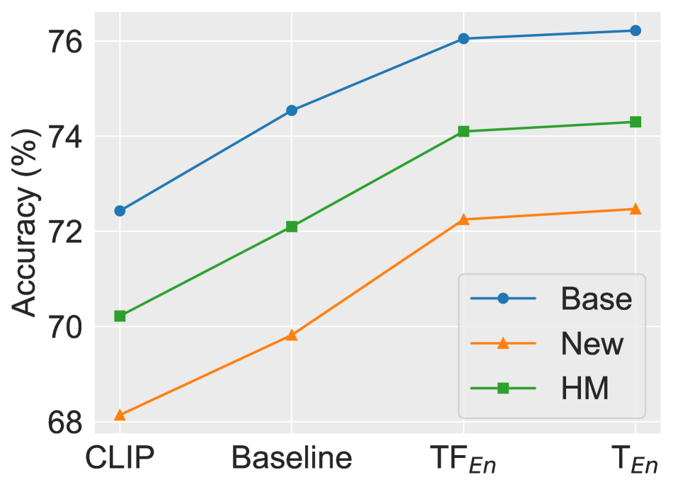
(a) Base-to-new performance

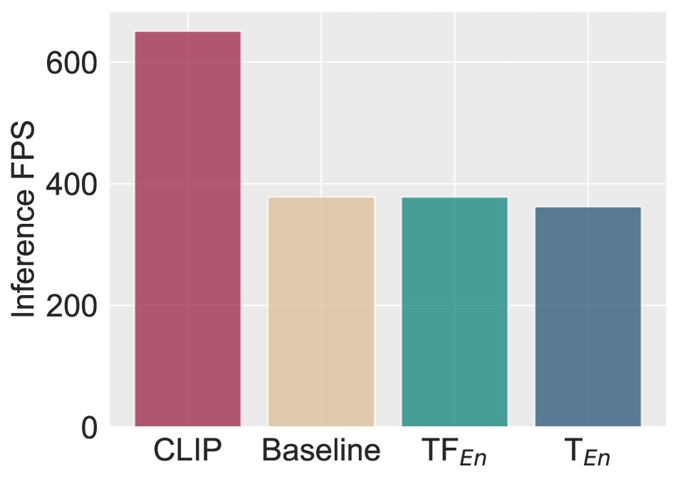
(b) Inference FPS

Figure 6: Comparing our ensemble strategies to baseline in terms of performance and inference time. Baseline uses the mean of the logits from four models as the final prediction.

4.4.1 Further Analysis

Ensemble Strategies

In Figure 6, we compare the performance and inference FPS with two baselines: zero-shot CLIP-ViT-B/16 (CLIP) and mean of the logits from four CLIP models (Baseline). We found that both our TF_En and T_En can outperform Baseline with the comparable inference FPS, while achieving significant improvement over CLIP without sacrificing much inference time.

Ablation Study of SWIG

We conduct comprehensive ablation studies of our SWIG in Table 6. First, we adjust the number of SWIG’s outputs to three, representing the weights for three weak VLMs, while assigning a weight of 1.0 to CLIP-ViT-B/16. The performance was slightly inferior to using four weights. This suggests that tuning our SWIG on a given dataset can generate reasonable weights for the four models, with performance comparable to maintaining the dominance of CLIP-ViT-B/16. Second, we take the concatenated logits of four models as the input for our SWIG, but the performance is much worse as the SWIG is too biased on base classes as discussed in Sec 3.4. Finally, since SWIG consists of two linear layers: $f_{dim}\rightarrow f_{dim}/d_{s}$, $f_{dim}/d_{s}\rightarrow num_{weight}$, we ablate the downsampling scale $d_{s}$ and found that our SWIG is not sensitive to $d_{s}$.

Acc	# Output Weights		Input Type		Downsampling Scale
	3	4	Logits	Features	4	8	16	32	64
Base	76.11	76.22	75.45	76.22	76.16	76.18	76.16	76.22	76.18
New	72.38	72.47	71.54	72.47	72.36	72.37	72.42	72.47	72.34
HM	74.20	74.30	73.44	74.30	74.21	74.23	74.24	74.30	74.21

Table 6: Ablation Study of our SWIG in terms of the number of output weights, input type and downsampling scales of middle layer on ImageNet.

4.5 Cross-dataset Evaluation

Table 5 presents the results of cross-dataset evaluation for state-of-the-art methods. In general, our tuning ensemble demonstrates the best overall performance, surpassing other methods on 8 out of 10 datasets. Several noteworthy observations are discussed below. First, we observe that previous methods with intricate designs tend to overfit on the training dataset, leading to sub-optimal performance on other datasets. For instance, CoOp achieves the highest performance on ImageNet yet the lowest averaged accuracy over 10 datasets. Second, the zero-shot CLIP model, trained on a million-level paired data, already achieves impressive performance on diverse datasets, which is slightly worse than existing SOTA methods.

5 Conclusion

This paper represents the pioneering exploration of leveraging much weaker Vision-Language Models (VLMs) collaboratively to enhance the performance of a single robust one. Three tailored ensemble strategies are introduced, addressing distinct scenarios. Firstly, the zero-shot ensemble dynamically adjusts logits based on model confidence when relying solely on pre-trained VLMs. Furthermore, for scenarios with additional few-shot samples, we propose both training-free and tuning ensembles, providing flexibility based on computing resource availability. Extensive experiments demonstrate the superiority of the proposed ensembles. Importantly, this work establishes a novel pathway for improved generalization in VLMs through ensemble learning, serving as a positive inspiration for future research endeavors.

Supplementary Material

We provide additional content to enhance the understanding of our method, which is listed as follows:

• Section 6 offers more experimental results, including the evaluation on domain generalization and effect of our tuning ensemble on state-of-the-art methods.

• Section 7 presents the broader impact of our method, including some insightful findings and the significance of our work to the community.

• Section 8 shows the limitations of our method, inspiring the future works.

6 More Experiments

6.1 Domain Generalization

We provide the comparison results of existing methods on domain generalization in Table 7. Overall, the best performance is achieved by using our tuning ensemble T_En on CoCoOp, with the accuracy gain 1.75%. This further indicates the importance of ensemble learning on enhanced generalization of pre-trained vision-language models. Moreover, we found that CLIP + T_En shows much better performance than CLIP only, but is worse than other state-of-the-art generalization methods. This differs from the finding in the cross-dataset generalization, where CLIP + T_En surpasses other SOTA methods by large margins. The reason is that domain and cross-dataset generalization evaluate the model in distinct aspects. Concretely, cross-dataset generalization is more challenging as it requires the model trained on one dataset to perform well on other datasets with unseen classes and domains, while domain generalization considers domain transfer only. Another interesting observation is that our method can perform consistently better on both source and target domains. This stands in stark contrast to prior methods, which often excel in the source domain but exhibit a notable decline in performance when applied to the target domain. For instance, methods like CoOp may outperform others in the source domain but degrade when confronted with the target domain.

	Source	Target
	ImageNet	-V2	-S	-A	-R	Avg.
CLIP [51]	66.73	60.83	46.15	47.77	73.96	57.18
CoOp [73]	71.51	64.20	47.99	49.71	75.21	59.28
CoCoOp [72]	71.02	64.07	48.75	50.63	76.18	59.91
MaPLe [34]	70.72	64.07	49.15	50.90	76.98	60.28
PromptSRC [35]	71.27	64.35	49.55	50.90	77.80	60.65
CLIP + TEn	70.88	62.87	48.97	49.97	75.98	59.45
CoCoOp + TEn	73.25	65.73	50.70	52.11	78.11	61.66

Table 7: Comparison with existing methods in domain generalization set-up. Our CoCoOp + T_En shows the best performance on all target datasets.

6.2 Effect of Tuning Ensemble

Since we have analyzed the effect of using tuning ensemble T_En on CLIP in main text, we further show its effect on other state-of-the-art methods in Table 8, namely CoCoOp (CVPR22)[72] and PromptSRC (ICCV23) [35]. In general, our T_En consistently demonstrates superior performance when compared to both the baseline model and its naïve ensemble counterpart. This trend underscores the efficacy of our method in effectively harnessing knowledge from multiple models. We also found that CoCoOp + T_En outperforms PromptSRC + T_En in some cases, e.g., 75.49% vs. 75.04% on ImageNet. This is attributed to the advantage of employing more ensemble models, showcasing the effectiveness of our T_En in leveraging the collective power of multiple models.

	Average			ImageNet [10]			Caltech101 [16]			OxfordPets [50]
	Base	New	HM	Base	New	HM	Base	New	HM	Base	New	HM
CoCoOp† [72]	80.14	71.55	75.60	76.05	70.61	73.23	97.91	93.99	95.91	95.41	97.54	96.46
CoCoOp + MeanEn	83.20	74.42	78.57	77.57	72.20	74.79	98.13	95.49	96.79	95.43	98.04	96.72
CoCoOp + TEn	83.56	75.27	79.20	78.39	72.79	75.49	98.32	95.74	97.01	95.69	98.27	96.96
PromptSRC† [35]	83.81	75.69	79.54	77.57	70.22	73.71	98.06	93.96	95.97	94.59	97.15	95.85
PromptSRC + MeanEn	85.12	76.63	80.65	78.14	71.42	74.63	98.45	95.25	96.82	95.55	97.62	96.57
PromptSRC + TEn	85.48	77.17	81.11	78.74	71.68	75.04	98.58	95.74	97.14	95.96	97.71	96.83

	StanfordCars [36]			Flowers102 [49]			Food101 [2]			FGVCAircraft [44]
	Base	New	HM	Base	New	HM	Base	New	HM	Base	New	HM
CoCoOp† [72]	71.01	73.81	72.38	93.86	72.03	81.51	90.55	91.32	90.93	33.43	24.71	28.42
CoCoOp + MeanEn	78.23	78.46	78.34	97.69	75.93	85.45	90.85	91.89	91.37	36.39	27.05	31.03
CoCoOp + TEn	78.69	78.73	78.71	97.82	77.23	86.31	90.93	92.03	91.48	36.51	30.17	33.04
PromptSRC† [35]	79.19	75.45	77.27	97.63	77.07	86.14	90.35	91.46	90.90	42.73	35.63	38.86
PromptSRC + MeanEn	80.80	78.31	79.54	98.74	77.07	86.57	90.56	91.55	91.05	42.50	34.17	37.88
PromptSRC + TEn	81.26	78.48	79.85	98.77	77.52	86.86	90.75	91.70	91.22	43.22	36.47	39.56

	SUN397 [66]			DTD [7]			EuroSAT [27]			UCF101 [57]
	Base	New	HM	Base	New	HM	Base	New	HM	Base	New	HM
CoCoOp† [72]	79.46	77.24	78.33	76.01	54.99	63.81	86.10	56.49	68.22	81.73	74.27	77.82
CoCoOp + MeanEn	81.61	80.41	81.01	81.02	61.15	69.70	93.77	62.15	74.75	84.54	75.88	79.98
CoCoOp + TEn	81.96	80.63	81.29	81.37	62.01	70.38	94.38	64.18	76.40	85.13	76.15	80.39
PromptSRC† [35]	82.37	78.91	80.60	81.56	61.35	70.03	90.96	73.90	81.55	86.92	77.50	81.94
PromptSRC + MeanEn	83.65	80.36	81.97	84.38	62.72	71.96	95.09	76.02	84.49	88.42	78.46	83.14
PromptSRC + TEn	83.88	80.86	82.34	84.72	63.16	72.37	95.52	76.41	84.90	88.83	79.10	83.68

Table 8: Effect of using tuning ensemble T_En on state-of-the-art methods. When employing our T_En, four of CoCoOp models, i.e., RN50, RN101, ViT-B/32 and ViT-B/16, are utilized, while only two ViT-based models for PromptSRC as it is explicitly designed for ViT. ${\dagger}$: reproduced by the official code. Mean_En: averaging the predictions of individual models. The best accuracy is in bold.

7 Broader Impact

This work pioneers the application of ensemble learning to enhance the generalization of vision-language models (VLMs) and offers three simple yet effective ensemble strategies, providing valuable insights to improve the generalization of pre-trained VLMs. More importantly, we made several interesting observations: (i) the “weak” VLMs, displaying substantial performance gaps compared to a strong individual VLM, can serve as valuable contributors in ensemble learning. (ii) contrary to the conventional wisdom that larger model sizes equate to better performance, we identified instances, particularly with ResNet-based [26] vision encoders for CLIP [51], where this expectation does not always hold. (iii) Zero-shot CLIP exhibits impressive generalization capabilities on unseen scenarios. Optimally harnessing this power can even surpass the performance of specifically designed generalization methods. In essence, our work provides fresh insights into the realm of ensemble learning for generalized VLMs and offers valuable findings that can contribute to advancements in the field.

8 Limitations

In this work, we take the initial stride towards incorporating ensemble learning into the generalization of VLMs. Our focus is on delineating potential avenues for leveraging ensemble strategies to enhance the performance of VLMs in generalized scenarios. However, it is essential to note that our exploration, at this juncture, only scratches the surface of the capabilities that ensemble learning might offer. Fully harnessing the power of ensemble learning in the context of VLM generalization represents a promising avenue for future investigation.

References

- Anderson et al. [2018] Peter Anderson, Xiaodong He, Chris Buehler, Damien Teney, Mark Johnson, Stephen Gould, and Lei Zhang. Bottom-up and top-down attention for image captioning and visual question answering. In CVPR, pages 6077–6086, 2018.
- Bossard et al. [2014] Lukas Bossard, Matthieu Guillaumin, and Luc Van Gool. Food-101–mining discriminative components with random forests. In ECCV, pages 446–461. Springer, 2014.
- Breiman [1996] Leo Breiman. Bagging predictors. Machine learning, 24:123–140, 1996.
- Breiman [2001] Leo Breiman. Random forests. Machine learning, 45:5–32, 2001.
- Buja and Stuetzle [2000] Andreas Buja and Werner Stuetzle. Smoothing effects of bagging. Preprint. AT&T Labs-Research, 2000.
- Chao et al. [2016] Wei-Lun Chao, Soravit Changpinyo, Boqing Gong, and Fei Sha. An empirical study and analysis of generalized zero-shot learning for object recognition in the wild. In ECCV, pages 52–68. Springer, 2016.
- Cimpoi et al. [2014] Mircea Cimpoi, Subhransu Maji, Iasonas Kokkinos, Sammy Mohamed, and Andrea Vedaldi. Describing textures in the wild. In CVPR, pages 3606–3613, 2014.
- Coates and Ng [2011] Adam Coates and Andrew Y Ng. The importance of encoding versus training with sparse coding and vector quantization. In ICML, 2011.
- Cortes et al. [2014] Corinna Cortes, Mehryar Mohri, and Umar Syed. Deep boosting. In ICML, pages 1179–1187. PMLR, 2014.
- Deng et al. [2009] Jia Deng, Wei Dong, Richard Socher, Li-Jia Li, Kai Li, and Li Fei-Fei. Imagenet: A large-scale hierarchical image database. In CVPR, pages 248–255. Ieee, 2009.
- Deng et al. [2012] Li Deng, Dong Yu, and John Platt. Scalable stacking and learning for building deep architectures. In ICASSP, pages 2133–2136. IEEE, 2012.
- Desai and Johnson [2021] Karan Desai and Justin Johnson. Virtex: Learning visual representations from textual annotations. In CVPR, pages 11162–11173, 2021.
- Dosovitskiy et al. [2020] Alexey Dosovitskiy, Lucas Beyer, Alexander Kolesnikov, Dirk Weissenborn, Xiaohua Zhai, Thomas Unterthiner, Mostafa Dehghani, Matthias Minderer, Georg Heigold, Sylvain Gelly, et al. An image is worth 16x16 words: Transformers for image recognition at scale. In ICLR, 2020.
- Dosovitskiy et al. [2021] Alexey Dosovitskiy, Lucas Beyer, Alexander Kolesnikov, Dirk Weissenborn, Xiaohua Zhai, Thomas Unterthiner, Mostafa Dehghani, Matthias Minderer, Georg Heigold, Sylvain Gelly, Jakob Uszkoreit, and Neil Houlsby. An image is worth 16x16 words: Transformers for image recognition at scale. ICLR, 2021.
- Elhoseiny et al. [2013] Mohamed Elhoseiny, Babak Saleh, and Ahmed Elgammal. Write a classifier: Zero-shot learning using purely textual descriptions. In ICCV, pages 2584–2591, 2013.
- Fei-Fei et al. [2004] Li Fei-Fei, Rob Fergus, and Pietro Perona. Learning generative visual models from few training examples: An incremental bayesian approach tested on 101 object categories. In CVPRW, pages 178–178. IEEE, 2004.
- Freund et al. [1996] Yoav Freund, Robert E Schapire, et al. Experiments with a new boosting algorithm. In ICML, pages 148–156. Citeseer, 1996.
- Friedman [2001] Jerome H Friedman. Greedy function approximation: a gradient boosting machine. Annals of statistics, pages 1189–1232, 2001.
- Frome et al. [2013] Andrea Frome, Greg S Corrado, Jon Shlens, Samy Bengio, Jeff Dean, Marc’Aurelio Ranzato, and Tomas Mikolov. Devise: A deep visual-semantic embedding model. NeurIPS, 26, 2013.
- Gan et al. [2017] Zhe Gan, Chuang Gan, Xiaodong He, Yunchen Pu, Kenneth Tran, Jianfeng Gao, Lawrence Carin, and Li Deng. Semantic compositional networks for visual captioning. In CVPR, pages 5630–5639, 2017.
- Gao et al. [2021] Peng Gao, Shijie Geng, Renrui Zhang, Teli Ma, Rongyao Fang, Yongfeng Zhang, Hongsheng Li, and Yu Qiao. Clip-adapter: Better vision-language models with feature adapters. arXiv preprint arXiv:2110.04544, 2021.
- Gomez et al. [2017] Lluis Gomez, Yash Patel, Marçal Rusinol, Dimosthenis Karatzas, and CV Jawahar. Self-supervised learning of visual features through embedding images into text topic spaces. In CVPR, pages 4230–4239, 2017.
- Goyal et al. [2017] Yash Goyal, Tejas Khot, Douglas Summers-Stay, Dhruv Batra, and Devi Parikh. Making the v in vqa matter: Elevating the role of image understanding in visual question answering. In CVPR, pages 6904–6913, 2017.
- Gurari et al. [2018] Danna Gurari, Qing Li, Abigale J Stangl, Anhong Guo, Chi Lin, Kristen Grauman, Jiebo Luo, and Jeffrey P Bigham. Vizwiz grand challenge: Answering visual questions from blind people. In CVPR, pages 3608–3617, 2018.
- Ha et al. [2005] Kyoungnam Ha, Sungzoon Cho, and Douglas MacLachlan. Response models based on bagging neural networks. Journal of Interactive Marketing, 19(1):17–30, 2005.
- He et al. [2016] Kaiming He, Xiangyu Zhang, Shaoqing Ren, and Jian Sun. Deep residual learning for image recognition. In CVPR, pages 770–778, 2016.
- Helber et al. [2019] Patrick Helber, Benjamin Bischke, Andreas Dengel, and Damian Borth. Eurosat: A novel dataset and deep learning benchmark for land use and land cover classification. IEEE Journal of Selected Topics in Applied Earth Observations and Remote Sensing, 12(7):2217–2226, 2019.
- Huynh and Elhamifar [2020] Dat Huynh and Ehsan Elhamifar. Fine-grained generalized zero-shot learning via dense attribute-based attention. In CVPR, pages 4483–4493, 2020.
- Jia et al. [2021] Chao Jia, Yinfei Yang, Ye Xia, Yi-Ting Chen, Zarana Parekh, Hieu Pham, Quoc Le, Yun-Hsuan Sung, Zhen Li, and Tom Duerig. Scaling up visual and vision-language representation learning with noisy text supervision. In ICML, pages 4904–4916. PMLR, 2021.
- Jiang et al. [2020] Zhengbao Jiang, Frank F Xu, Jun Araki, and Graham Neubig. How can we know what language models know? ACL, 8:423–438, 2020.
- Johnson et al. [2017] Justin Johnson, Bharath Hariharan, Laurens Van Der Maaten, Li Fei-Fei, C Lawrence Zitnick, and Ross Girshick. Clevr: A diagnostic dataset for compositional language and elementary visual reasoning. In CVPR, pages 2901–2910, 2017.
- Joulin et al. [2016] Armand Joulin, Laurens van der Maaten, Allan Jabri, and Nicolas Vasilache. Learning visual features from large weakly supervised data. In ECCV, pages 67–84. Springer, 2016.
- Kang et al. [2020] Tianyu Kang, Ping Chen, John Quackenbush, and Wei Ding. A novel deep learning model by stacking conditional restricted boltzmann machine and deep neural network. In SIGKDD, pages 1316–1324, 2020.
- Khattak et al. [2023a] Muhammad Uzair Khattak, Hanoona Rasheed, Muhammad Maaz, Salman Khan, and Fahad Shahbaz Khan. Maple: Multi-modal prompt learning. In CVPR, pages 19113–19122, 2023a.
- Khattak et al. [2023b] Muhammad Uzair Khattak, Syed Talal Wasim, Muzammal Naseer, Salman Khan, Ming-Hsuan Yang, and Fahad Shahbaz Khan. Self-regulating prompts: Foundational model adaptation without forgetting. In ICCV, pages 15190–15200, 2023b.
- Krause et al. [2013] Jonathan Krause, Michael Stark, Jia Deng, and Li Fei-Fei. 3d object representations for fine-grained categorization. In ICCVW, pages 554–561, 2013.
- LeBlanc and Tibshirani [1996] Michael LeBlanc and Robert Tibshirani. Combining estimates in regression and classification. Journal of the American Statistical Association, 91(436):1641–1650, 1996.
- Lei Ba et al. [2015] Jimmy Lei Ba, Kevin Swersky, Sanja Fidler, et al. Predicting deep zero-shot convolutional neural networks using textual descriptions. In ICCV, pages 4247–4255, 2015.
- Li et al. [2017] Ang Li, Allan Jabri, Armand Joulin, and Laurens Van Der Maaten. Learning visual n-grams from web data. In ICCV, pages 4183–4192, 2017.
- Li et al. [2023] Xin Li, Dongze Lian, Zhihe Lu, Jiawang Bai, Zhibo Chen, and Xinchao Wang. Graphadapter: Tuning vision-language models with dual knowledge graph. In NeurIPS, 2023.
- Li et al. [2021] Yangguang Li, Feng Liang, Lichen Zhao, Yufeng Cui, Wanli Ouyang, Jing Shao, Fengwei Yu, and Junjie Yan. Supervision exists everywhere: A data efficient contrastive language-image pre-training paradigm. arXiv preprint arXiv:2110.05208, 2021.
- Lu et al. [2017] Jiasen Lu, Caiming Xiong, Devi Parikh, and Richard Socher. Knowing when to look: Adaptive attention via a visual sentinel for image captioning. In CVPR, pages 375–383, 2017.
- Lu et al. [2022] Yuning Lu, Jianzhuang Liu, Yonggang Zhang, Yajing Liu, and Xinmei Tian. Prompt distribution learning. In CVPR, pages 5206–5215, 2022.
- Maji et al. [2013] Subhransu Maji, Esa Rahtu, Juho Kannala, Matthew Blaschko, and Andrea Vedaldi. Fine-grained visual classification of aircraft. arXiv preprint arXiv:1306.5151, 2013.
- Marino et al. [2019] Kenneth Marino, Mohammad Rastegari, Ali Farhadi, and Roozbeh Mottaghi. Ok-vqa: A visual question answering benchmark requiring external knowledge. In CVPR, pages 3195–3204, 2019.
- Mikolov et al. [2013a] Tomas Mikolov, Kai Chen, Greg Corrado, and Jeffrey Dean. Efficient estimation of word representations in vector space. In ICLR, 2013a.
- Mikolov et al. [2013b] Tomas Mikolov, Ilya Sutskever, Kai Chen, Greg S Corrado, and Jeff Dean. Distributed representations of words and phrases and their compositionality. NeurIPS, 26, 2013b.
- Nichol et al. [2021] Alex Nichol, Prafulla Dhariwal, Aditya Ramesh, Pranav Shyam, Pamela Mishkin, Bob McGrew, Ilya Sutskever, and Mark Chen. Glide: Towards photorealistic image generation and editing with text-guided diffusion models. arXiv preprint arXiv:2112.10741, 2021.
- Nilsback and Zisserman [2008] Maria-Elena Nilsback and Andrew Zisserman. Automated flower classification over a large number of classes. In ICCVGIP, pages 722–729. IEEE, 2008.
- Parkhi et al. [2012] Omkar M Parkhi, Andrea Vedaldi, Andrew Zisserman, and CV Jawahar. Cats and dogs. In CVPR, pages 3498–3505. IEEE, 2012.
- Radford et al. [2021] Alec Radford, Jong Wook Kim, Chris Hallacy, Aditya Ramesh, Gabriel Goh, Sandhini Agarwal, Girish Sastry, Amanda Askell, Pamela Mishkin, Jack Clark, et al. Learning transferable visual models from natural language supervision. In ICML, pages 8748–8763. PMLR, 2021.
- Ramesh et al. [2021] Aditya Ramesh, Mikhail Pavlov, Gabriel Goh, Scott Gray, Chelsea Voss, Alec Radford, Mark Chen, and Ilya Sutskever. Zero-shot text-to-image generation. In ICML, pages 8821–8831. PMLR, 2021.
- Sariyildiz et al. [2020] Mert Bulent Sariyildiz, Julien Perez, and Diane Larlus. Learning visual representations with caption annotations. In ECCV, pages 153–170. Springer, 2020.
- Shin et al. [2020] Taylor Shin, Yasaman Razeghi, Robert L Logan IV, Eric Wallace, and Sameer Singh. Autoprompt: Eliciting knowledge from language models with automatically generated prompts. In EMNLP, 2020.
- Singh et al. [2019] Amanpreet Singh, Vivek Natarajan, Meet Shah, Yu Jiang, Xinlei Chen, Dhruv Batra, Devi Parikh, and Marcus Rohrbach. Towards vqa models that can read. In CVPR, pages 8317–8326, 2019.
- Socher et al. [2013] Richard Socher, Milind Ganjoo, Christopher D Manning, and Andrew Ng. Zero-shot learning through cross-modal transfer. NeurIPS, 26, 2013.
- Soomro et al. [2012] Khurram Soomro, Amir Roshan Zamir, and Mubarak Shah. Ucf101: A dataset of 101 human actions classes from videos in the wild. arXiv preprint arXiv:1212.0402, 2012.
- Suhr et al. [2017] Alane Suhr, Mike Lewis, James Yeh, and Yoav Artzi. A corpus of natural language for visual reasoning. In ACL, pages 217–223, 2017.
- Torresani et al. [2010] Lorenzo Torresani, Martin Szummer, and Andrew Fitzgibbon. Efficient object category recognition using classemes. In ECCV, pages 776–789. Springer, 2010.
- Touvron et al. [2021] Hugo Touvron, Matthieu Cord, Matthijs Douze, Francisco Massa, Alexandre Sablayrolles, and Hervé Jégou. Training data-efficient image transformers & distillation through attention. In ICML, pages 10347–10357. PMLR, 2021.
- Vaswani et al. [2017] Ashish Vaswani, Noam Shazeer, Niki Parmar, Jakob Uszkoreit, Llion Jones, Aidan N Gomez, Łukasz Kaiser, and Illia Polosukhin. Attention is all you need. NeurIPS, 30, 2017.
- Wang et al. [2019] Wei Wang, Vincent W Zheng, Han Yu, and Chunyan Miao. A survey of zero-shot learning: Settings, methods, and applications. TIST, 10(2):1–37, 2019.
- Wang et al. [2023] Zhengbo Wang, Jian Liang, Ran He, Nan Xu, Zilei Wang, and Tieniu Tan. Improving zero-shot generalization for clip with synthesized prompts. In CVPR, pages 3032–3042, 2023.
- Wolpert [1992] David H Wolpert. Stacked generalization. Neural networks, 5(2):241–259, 1992.
- Xian et al. [2017] Yongqin Xian, Bernt Schiele, and Zeynep Akata. Zero-shot learning-the good, the bad and the ugly. In CVPR, pages 4582–4591, 2017.
- Xiao et al. [2010] Jianxiong Xiao, James Hays, Krista A Ehinger, Aude Oliva, and Antonio Torralba. Sun database: Large-scale scene recognition from abbey to zoo. In CVPR, pages 3485–3492. IEEE, 2010.
- Yi et al. [2022] Kai Yi, Xiaoqian Shen, Yunhao Gou, and Mohamed Elhoseiny. Exploring hierarchical graph representation for large-scale zero-shot image classification. In ECCV, pages 116–132. Springer, 2022.
- Yu et al. [2023] Tao Yu, Zhihe Lu, Xin Jin, Zhibo Chen, and Xinchao Wang. Task residual for tuning vision-language models. In CVPR, pages 10899–10909, 2023.
- Zellers et al. [2019] Rowan Zellers, Yonatan Bisk, Ali Farhadi, and Yejin Choi. From recognition to cognition: Visual commonsense reasoning. In CVPR, pages 6720–6731, 2019.
- Zhang et al. [2022] Renrui Zhang, Zhang Wei, Rongyao Fang, Peng Gao, Kunchang Li, Jifeng Dai, Yu Qiao, and Hongsheng Li. Tip-adapter: Training-free adaption of clip for few-shot classification. In ECCV, 2022.
- Zhong et al. [2021] Zexuan Zhong, Dan Friedman, and Danqi Chen. Factual probing is [mask]: Learning vs. learning to recall. In NAACL, 2021.
- Zhou et al. [2022a] Kaiyang Zhou, Jingkang Yang, Chen Change Loy, and Ziwei Liu. Conditional prompt learning for vision-language models. In CVPR, pages 16816–16825, 2022a.
- Zhou et al. [2022b] Kaiyang Zhou, Jingkang Yang, Chen Change Loy, and Ziwei Liu. Learning to prompt for vision-language models. IJCV, 130(9):2337–2348, 2022b.