DepthSSC: Depth-Spatial Alignment and Dynamic Voxel Resolution for Monocular 3D Semantic Scene Completion

Abstract

The task of 3D semantic scene completion with monocular cameras is gaining increasing attention in the field of autonomous driving. Its objective is to predict the occupancy status of each voxel in the 3D scene from partial image inputs. Despite the existence of numerous methods, many of them overlook the issue of accurate alignment between spatial and depth information. To address this, we propose DepthSSC, an advanced method for semantic scene completion solely based on monocular cameras. DepthSSC combines the ST-GF (Spatial Transformation Graph Fusion) module with geometric-aware voxelization, enabling dynamic adjustment of voxel resolution and considering the geometric complexity of 3D space to ensure precise alignment between spatial and depth information. This approach successfully mitigates spatial misalignment and distortion issues observed in prior methods. Through evaluation on the SemanticKITTI dataset, DepthSSC not only demonstrates its effectiveness in capturing intricate 3D structural details but also achieves state-of-the-art performance. We believe DepthSSC provides a fresh perspective on monocular camera-based 3D semantic scene completion research and anticipate it will inspire further related studies.

1 Introduction

3D Semantic Scene Completion (SSC) [19] plays a pivotal role in the domain of autonomous driving. It encompasses the task of predicting the occupancy of each voxel in a 3D scene using partial input from imaging devices. The initial exploration of this domain was spearheaded by SSCNet [19], which paved the way for subsequent methodologies employing 3D geometric data, encompassing depth perception and LiDAR-generated point clouds, to reconstruct scenes. In more recent developments, there’s been a notable pivot towards vision-centric methodologies in the context of autonomous driving perception. This shift is exemplified by the works of MonoScene [3], NDC-Scene [26] and OccDepth [15], which have delved into the transposition of two-dimensional image attributes into three-dimensional spaces, leveraging the power of 3D convolutional networks. Advancements have also been observed with TPVFormer [7] and VoxFormer [13], which integrate Transformer architectures for the adaptive extraction of voxel features, significantly enhancing the fidelity of scene modeling. Additionally, both Occ3D [20] and OccFormer [30] have introduced innovative approaches with their coarse-to-fine architectural designs and unique class-specific mask prediction strategies.

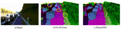
Figure 1: Comparison of VoxFormer [13] and our DepthSSC. The DepthSSC exhibits a significant advantage over VoxFormer in predicting occupied grids for both nearby small objects and distant objects. As shown in the yellow circled part of Figure 1(b), VoxFormer experiences notable issues with misrecognition and non-recognition. We hypothesize that these problems are attributable to VoxFormer’s lack of an essential mechanism to address the geometric complexity inherent in real-world 3D environments. More precisely, there is a mismatch between the geometric information of the scene and the query proposals.

However, previous visual approaches [3, 13, 26] have often grappled with challenges related to the accurate alignment of spatial and depth information, especially when working with data from monocular cameras. The inherent constraints of these cameras, including the lack of stereoscopic depth perception and limited field of view, often result in spatial misalignments, distortions, and deformations in the reconstructed 3D scenes. This leads to sub-optimal performance in tasks that require a high degree of spatial precision and resolution, such as object detection, path planning, and obstacle avoidance in autonomous driving scenarios.

Furthermore, while Transformer-based architectures like TPVFormer [7] and VoxFormer [13] have showcased potential in adaptively extracting voxel features, they still lack mechanisms to consider the geometric complexity inherent in real-world 3D environments. Often, uniform voxel resolutions are applied across different regions of a scene, neglecting the varied resolutions needed to accurately capture intricate details and structures. This oversight can lead to the loss of crucial information in areas of high geometric complexity, while also allocating unnecessary computational resources to simpler regions.

In light of these challenges, our work introduces DepthSSC, a novel method that seeks to bridge the existing gaps in monocular SSC. DepthSSC uniquely combines the power of spatial transformation with geometric awareness, ensuring accurate spatial-depth alignment and dynamic voxel resolution adaptation. By integrating the ST-GF (Spatially-Transformed Graph Fusion) module and the Geometrically-aware Voxelization technique, our approach diligently aligns spatial information with depth cues and dynamically adjusts voxel resolutions based on the geometric intricacies of the scene.

In order to evaluate DepthSSC, we conducted extensive experiments on SemanticKITTI [1] dataset and achieved superior performance. Ablation studies confirmed the effectiveness of the Spatially-Transformed Graph Fusion and Geometrically-aware Voxelization. Our key contributions can be summarized as follows:

• We introduce the Spatially-Transformed Graph Fusion module, which facilitates the spatial transformation and feature fusion from voxels to graph structures, ensuring precise alignment of spatial and depth information within the same spatial framework.

• We propose Geometrically-aware Voxelization, a method that considers the geometric complexity of 3D space, allowing for dynamic adjustments of voxel resolution to adapt to various regions.

• The proposed DepthSSC model achieves state-of-the-art results with 13.11 mIoU and 44.58 IoU on the SemanticKITTI benchmark, surpassing the latest approaches. Additionally, it demonstrates superior performance across different ranges on the SSCBench-KITTI-360 dataset. These results underline the importance of aligning depth information with scene information.

2 Related Work

3D Semantic Scene Completion.

A comprehensive understanding of 3D scenes is crucial for many application domains, such as robotic perception [27], autonomous driving [25], and digital twins. SSCNet [19] indicates that semantic segmentation and scene completion are not independent processes. Their semantic and geometric information are intricately intertwined and mutually reinforcing. This interplay has led to the concept of Semantic Scene Completion (SSC). Currently, 3D semantic scene completion methods can be categorized into three main types based on the nature of the input data: methods based on depth maps [29, 21, 10], methods combining depth maps with RGB images [11, 9], methods based on point clouds [4, 17], and methods based on RGB images [3, 13, 26]. Depth map-based SSC algorithms typically use a single depth map as input, concurrently predicting voxel grid occupancy and semantic labels. However, these methods do not fully utilize the rich color and texture information contained in RGB images. Consequently, models like TS3D [5] employ a dual-stream network architecture, using RGB images as an important supplement to depth maps to further enhance the performance of 3D semantic scene completion. SSC networks based on point cloud inputs exhibit superior performance on large-scale outdoor scene datasets compared to image-based methods, yet existing point cloud processing techniques lack a universally recognized feature extraction paradigm. Recently, SSC methods based on RGB images have gained attention. The low-cost nature of these methods holds significant potential for real-world applications.

Monocular 3D Semantic Scene Completion.

The task of completing a 3D scene using only RGB images presents significant challenges. A prominent strategy involves converting two-dimensional features into a three-dimensional context. This concept was initially explored in studies like MonoScene [3] and OccDepth [15], which project 2D features into 3D spaces using depth perception techniques. Concurrently, methods such as those employed by BEVFormer [14] aggregate 2D features directly within a 3D space, utilizing a query-based mechanism, as seen in TPVFormer [7], and SurroundOcc [22]. VoxFormer [13] begins with the sparse assembly of visible and occupied voxel queries based on depth estimations [28], subsequently expanding these sparse voxels into a dense 3D voxel structure. In our research, we introduce DepthSSC, a method that ensures precise spatial-depth alignment and adapts voxel density according to scene requirements. This approach lays the foundation for enhancing local prediction performance in monocular image scene completion.

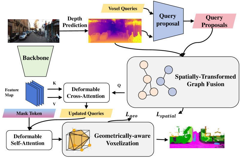
Figure 2: Architecture of the DepthSSC. The process begins with a backbone extracting 2D features from an input image, followed by the projection of 2D features into the 3D voxel domain through deformable self-attention and deformable cross-attention mechanisms, integrating spatial and geometric information. The Spatially-Transformed Graph Fusion (ST-GF) module enhances spatial alignment and feature fusion within a graph structure formed from the voxel queries, employing a spatial transformer network (STN) for precise voxel localization and transformation. Geometrically-aware Voxelization (GAV) adapts voxel resolution based on geometric complexity, optimizing the model’s representational fidelity particularly in geometrically complex areas.

3 Method

In this part, we first introduce the baseline model VoxFormer [13] in Section 3.1, which is the current state-of-the-art model for single-camera semantic scene completion. Then, we will present two core modules, Spatially-Transformed Graph Fusion and Geometrically-aware Voxelization, in Sections 3.2 and 3.3, respectively.

3.1 Preliminary

VoxFormer, as an innovative architecture, elegantly addresses SSC by infusing the expressive power of Transformers with 3D voxel representations. This methodology is underpinned by the core concept of voxel queries, which serve as 3D grid-shaped learnable parameters that capture features from the 2D image domain and project them into the 3D voxel domain. This transition from 2D to 3D is achieved through camera projection matrices, allowing the model to intuit the 3D structure of the scene from 2D inputs.

The overall process of VoxFormer is architected in two stages: (i) the generation of class-agnostic query proposals, and (ii) the class-specific segmentation which propagates refined information throughout the voxel grid. The underlying backbone for 2D feature extraction is typically a ResNet-50 [6], a robust choice for extracting rich feature representations from input RGB images.

2D feature extraction.

From an input RGB image $I_{t}$, we extract 2D features $F_{2D_{t}}\in\mathbb{R}^{b\times c\times d}$ using a convolutional neural network backbone. where, $b\times c$ corresponds to the spatial resolution and $d$ is the dimension of the features.

Voxel Queries.

The voxel queries $Q\in\mathbb{R}^{h\times w\times z\times d}$ are predefined as 3D-grid-shaped learnable parameters. Each query $q\in\mathbb{R}^{d}$ located at a spatial position $(i,j,k)$ is tasked with mapping 2D image features to a voxel within the 3D volume, where $h\times w\times z$ is set to a lower spatial resolution than the desired output to reduce computational overhead.

Class-Agnostic Query Proposals.

A subset of voxel queries $Q_{p}=\mathrm{Reshape}(Q[M_{\mathrm{out}}])$ is selected based on predicted occupancy from depth information. $Q_{p}\in\mathbb{R}^{N_{p}\times d}$ and $M_{\text{out}}$ is the occupancy map after depth correction.

Class-Agnostic Query Proposals.

Deformable Cross-Attention (DCA) mechanism. This approach allows for flexible attention over a local neighborhood in the 2D feature space by proposing queries $Q_{p}$ with calculated offsets:

$$\small\texttt{DCA}(\mathbf{q}_{p},\mathbf{F}^{2D})=\frac{1}{|\mathcal{V}_{t}|}\sum_{t\in\mathcal{V}_{t}}\texttt{DA}(\mathbf{q}_{p},\mathcal{P}(\mathbf{p},t),\mathbf{F}_{t}^{2D}),$$ (1)

where $P(p,t)$ is the projection function that maps 3D points to the 2D plane of image $t$.

Deformable Self-Attention (DSA).

This attention mechanism refines voxel features by allowing them to interact within the 3D space:

$$\small\texttt{DSA}(\mathbf{F}^{3D},\mathbf{F}^{3D})=\texttt{DA}(\mathbf{f},\mathbf{p},\mathbf{F}^{3D}),$$ (2)

where $f$ can be either a mask token or an updated query proposal at location $p$.

Semantic Segmentation Output.

The final output $Y_{t}\in\mathbb{R}^{H\times W\times Z\times(M+1)}$ represents the semantic segmentation map. where $H\times W\times Z$ is the output resolution, and $M+1$ indicates $M$ semantic classes plus one void class.

3.2 Spatially-Transformed Graph Fusion

In the task of 3D SSC, both depth maps and voxel queries are crucial prediction components. However, since they are independently predicted by neural networks, even slight parameter variations can lead to spatial information shifts and deformations. These shifts and deformations can result in incomplete alignment between objects in the depth map and the spatial structures in voxel queries, thereby affecting the overall accuracy of the 3D representation.

To address this issue, we have designed the Spatially-Transformed Graph Fusion (ST-GF) module. The ST-GF module is aimed at achieving spatial transformation and feature fusion from voxels to graph structures, ensuring that spatial and depth information can be accurately aligned within the same spatial framework to optimize voxel semantic representations. This module first utilizes a spatial transformation network (STN) to perform spatial transformations on voxels. Subsequently, it constructs a graph structure using the transformed voxels and accomplishes feature fusion through a graph convolution network (GCN). Finally, the updated graph node features are back-propagated to the original voxels.

Voxel-to-Node Mapping.

The localization network with STN predicts spatial transformation parameters for each voxel, facilitating a better alignment of voxels with their actual three-dimensional structures. Based on these transformation parameters, accurate positioning and transformation of voxels in space are achieved. Given a voxel query $Q\in\mathbb{R}^{h\times w\times z\times d}$ and Depth Prediction $D\in\mathbb{R}^{h\times w\times z\times d^{\prime}}$, they are stacked in parallel to form a new voxel query $Q^{\prime}\in\mathbb{R}^{h\times w\times z\times(d+d^{\prime})}$.

The localization network, employing a Spatial Transformation Network (STN), predicts spatial transformation parameters $\Theta$ for each voxel. For each voxel query $q_{ijk}$, the Localization Network first outputs a 3D affine transformation matrix $\Theta$ as follows:

$$\Theta=LocNet(q_{ijk}).$$ (3)

Subsequently, using the transformation matrix $\Theta$, a grid generator produces a sampling grid from the output space to the input space. For each position $P_{out}$ in the output space, a corresponding position $P_{in}$ in the input space is generated as follows:

$$P_{in}=\Theta\times P_{out}.$$ (4)

A sampler utilizes the generated grid to perform sampling from the input data, employing trilinear (3D) interpolation as follows:

$$q_{ijk}^{\prime}=Trilinear(q_{ijk},P_{in}),$$ (5)

where, $q_{ijk}^{\prime}$ represents the transformed voxel position.

Voxel Clustering and Graph Structure Construction.

After spatial transformation, voxels are clustered based on their spatial similarity. Let $q_{ijk}^{\prime}$ represent the voxel after spatial transformation, with 3D coordinates $(i,j,k)$. Additionally, we consider the mean features of this voxel among its neighboring voxels. The mean neighbor features are calculated as follows:

$$q_{neigh}^{\prime} =\frac{1}{6}\left(q_{i+1,j,k}^{\prime}+q_{i-1,j,k}^{\prime}\right.$$

$$\quad\left.+q_{i,j+1,k}^{\prime}+q_{i,j-1,k}^{\prime}+q_{i,j,k+1}^{\prime}+q_{i,j,k-1}^{\prime}\right).$$ (6)

Therefore, spatial attributes can be computed as follows:

$$A_{ijk}^{\prime}=f(q_{ijk}^{\prime},\text{Coordinates}(i,j,k),\text{Neighbors}(q_{ijk}^{\prime})),$$ (7)

$$f(q_{ijk}^{\prime},(i,j,k),q_{neigh}^{\prime})=\alpha\cdot q_{ijk}^{\prime}+\beta\cdot(i,j,k)+\gamma\cdot q_{neigh}^{\prime},$$ (8)

where, $\alpha$, $\beta$, and $\gamma$ are weight parameters that can be learned through training. Their values determine the contribution of each component to the spatial attributes.

Next, we apply K-Means [8] or other clustering algorithms to cluster the spatial attributes $A_{ijk}^{\prime}$. Each cluster has a center denoted as $C_{m}$, where $m$ is the cluster index. We define a connection matrix $W$, where $W_{mn}$ represents the connection strength between nodes $C_{m}$ and $C_{n}$. The connection strength can be determined based on the Euclidean distance or other spatial similarity measures between the two centers:

$$W_{mn}=g(C_{m},C_{n}),$$ (9)

where, $g$ is a function used to calculate the spatial similarity between two nodes. In this paper, we employ Euclidean clustering for the computation of $g$.

Graph Fusion.

or each voxel within a cluster, we fuse their features as follows:

$$F_{C_{m}}=\frac{1}{|C_{m}|}\sum_{q_{ijk}\in C_{m}}q_{ijk}^{\prime},$$ (10)

where, $F_{C_{m}}$ represents the feature of node $C_{m}$, and $|C_{m}|$ is the number of voxels in cluster $C_{m}$.

Using the sampler in STN, we further optimize the spatial alignment of these fused features:

$$F_{C_{m}}^{*}=Sampler(F_{C_{m}},\Theta).$$ (11)

Then, we perform graph convolution operations on the fused and aligned features. Let $G(F,A)$ denote the graph convolution network, where $F$ is the feature matrix and $A$ is the adjacency matrix. The updated features for node $C_{m}$ are given by:

$$F_{C_{m}}^{\prime}=G(F_{C_{m}}^{*},A).$$ (12)

Feature Backpropagation.

Lastly, we propagate the features from the graph nodes back to the original voxels. Utilizing the inverse transformation operation with STN ensures that the features are accurately backpropagated to their original spatial locations, preserving spatial continuity of the features:

$$q_{ijk}^{*}=STN^{-1}(F_{C_{m}}^{\prime},\Theta),$$ (13)

where, $q_{ijk}^{*}$ represents the voxel features after the backward propagation.

		SC	SSC
Method	SSC Input	IoU	$\blacksquare$ road (15.30%)	$\blacksquare$ sidewalk (11.13%)	$\blacksquare$ parking (1.12%)	$\blacksquare$ other-grnd (0.56%)	$\blacksquare$ building (14.1%)	$\blacksquare$ car (3.92%)	$\blacksquare$ truck (0.16%)	$\blacksquare$ bicycle (0.03%)	$\blacksquare$ motorcycle (0.03%)	$\blacksquare$ other-veh. (0.20%)	$\blacksquare$ vegetation (39.3%)	$\blacksquare$ trunk (0.51%)	$\blacksquare$ terrain (%)	$\blacksquare$ person (0.07%)	$\blacksquare$ bicyclist (0.07%)	$\blacksquare$ motorcyclist. (0.05%)	$\blacksquare$ fence (3.90%)	$\blacksquare$ pole (0.29%)	$\blacksquare$ traf.-sign (0.08%)	mIoU
LMSCNet${}^{\text{rgb}}$ [18]	Occ	31.38	46.70	19.50	13.50	3.10	10.30	14.30	0.30	0.00	0.00	0.00	10.80	0.00	10.40	0.00	0.00	0.00	5.40	0.00	0.00	7.07
AICNet${}^{\text{rgb}}$ [11]	RGB & Depth	23.93	39.30	18.30	19.80	1.60	9.60	15.30	0.70	0.00	0.00	0.00	9.60	1.90	13.50	0.00	0.00	0.00	5.00	0.10	0.00	7.09
JS3C-Net${}^{\text{rgb}}$ [24]	Pts	34.00	47.30	21.70	19.90	2.80	12.70	20.10	0.80	0.00	0.00	4.10	14.20	3.10	12.40	0.00	0.20	0.20	8.70	1.90	0.30	8.97
MonoScene [3]	RGB	34.16	54.70	27.10	24.80	5.70	14.40	18.80	3.30	0.50	0.70	4.40	14.90	2.40	19.50	1.00	1.40	0.40	11.10	3.30	2.10	11.08
TPVFormer [11]	RGB	34.25	55.10	27.20	27.40	6.50	14.80	19.20	3.70	1.00	0.50	2.30	13.90	2.60	20.40	1.10	2.40	0.30	11.00	2.90	1.50	11.26
Voxformer [13]	RGB	42.95	53.90	25.30	21.10	5.60	19.80	20.80	3.50	1.00	0.70	3.70	22.40	7.50	21.30	1.40	2.60	0.20	11.10	5.10	4.90	12.20
NDC-Scene [26]	RGB	36.19	58.12	28.05	25.31	6.53	14.90	19.13	4.77	1.93	2.07	6.69	17.94	3.49	25.01	3.44	2.77	1.64	12.85	4.43	2.96	12.58
DepthSSC (ours)	RGB	44.58	55.64	27.25	25.72	5.78	20.46	21.94	3.74	1.35	0.98	4.17	23.37	7.64	21.56	1.34	2.79	0.28	12.94	5.87	6.23	13.11

Table 1: Quantitative comparison against RGB-inferred baselines and the state-of-the-art monocular SSC method on SemanticKITTI [1] (hidden test set).

3.3 Geometrically-aware Voxelization

Voxformer’s deformable self-attention aims to consider local regions within the 3D scene for richer visual features. However, using a fixed voxel resolution may not fully capture the details in geometrically complex areas. In such cases, the fixed voxel resolution can limit the model’s performance in handling these regions, especially in applications where precise modeling of geometry is required. To address this issue, we introduce Geometrically-aware Voxelization (GAV). This approach takes into account the geometric complexity in 3D space and allows for dynamic adjustments of voxel resolution. This way, in geometrically complex regions, we can use a higher voxel resolution to ensure the capture of all details, while in simpler regions, a lower resolution can be used to conserve computational resources and speed up model execution.

Geometric Complexity Assessment.

For a given three-dimensional voxel feature $S$, we use the Marching Cubes [16] algorithm to obtain the surface $M$. For each voxel $V_{i}$, we compute the number of intersections with the surface $M$ or the number of surface fragments contained within it: $C(V_{i})=\text{count of intersections of }V_{i}\text{ with }M$, where, $C(V_{i})$ represents the geometric complexity of voxel $V_{i}$.

For each voxel $V_{i}$, we map its geometric complexity $C(V_{i})$ to a continuous range representing its resolution:

$$R(V_{i})=f(C(V_{i})),$$ (14)

where $f$ is a sigmoid activation function.

Resolution-Adaptive Deformable Attention.

When performing deformable self-attention operations, we take into consideration the dynamic resolution $R(V_{i})$ of voxels. The resolution of voxels directly affects the position and quantity of query points in deformable self-attention, with higher resolution corresponding to finer query points. For each voxel $V_{i}$, its position in three-dimensional space can be represented as $p=(x,y,z)$. We can adjust these positions based on the resolution $R(V_{i})$, allowing voxels with higher complexity to have a higher query density. To achieve this, we introduce a mechanism for deformable attention.

First, we calculate the offset of query points as follows:

$$\Delta p=W_{p}\times f,$$ (15)

where, $W_{p}$ is a weight matrix, and $f$ can be a mask or an updated query proposal.

Next, we update the query point positions:

$$p^{\prime}=p+\delta\times R(V_{i})+\Delta p,$$ (16)

where $\delta$ is a constant that determines the strength of the influence of resolution $R(V_{i})$ on query point positions.

With the new query positions $p^{\prime}$, we further compute the updated queries $Q^{\prime}$ and calculate the deformable attention weights:

$$DA(f,p^{\prime},F_{3D})=\operatorname{softmax}\left(\frac{Q^{\prime}K^{T}}{\sqrt{d_{k}}}\right)V,$$ (17)

$$Q^{\prime}=W_{q}\times p^{\prime}.$$ (18)

The formula for obtaining refined voxel features $\hat{F_{3D}}$ using deformable self-attention is as follows:

$$\small DSA(F_{3D},F_{3D})=DA(f,p^{\prime},F_{3D})=\text{softmax}\left(\frac{Q^{\prime}K^{T}}{\sqrt{d_{k}}}\right)V.$$ (19)

By embedding the Spatially-Transformed Graph Fusion and Geometrically-aware Voxelization modules into Voxformer, we obtain the model presented in this paper: Geometrically-aware Voxelized Transformer with Spatially-Transformed Graph Fusion (DepthSSC).

3.4 Training Loss

For the first-stage training of the model, the primary focus is on the continuity of spatial information and occupancy prediction. Regarding occupancy prediction, binary cross-entropy loss is employed, which is used to predict occupancy at a lower spatial resolution. Simultaneously, to ensure the continuity and consistency of spatial information during the fusion process, it can be defined by comparing the distances between neighboring nodes:

$$L_{spatial}=\frac{1}{M}\sum_{j=1}^{M}\|d(G_{orig,j},G_{orig,j+1})$$

$$-d(G_{transformed,j},G_{transformed,j+1})\|.$$ (20)

where, $d()$ represents the distance function between two nodes, and $M$ is the total number of nodes. In the second stage, the model is trained for multi-class semantic voxel grid prediction. We utilize weighted cross-entropy loss and Scene-class Affinity Loss as the training objectives. Additionally, since Geometrically-aware Voxelization may affect the distribution of geometric information in voxel features, potentially leading to geometric shape distortion or detail loss, we define the Geometric Preservation Loss $L_{geo}$ based on the Hausdorff distance measure between the original 3D data points and the voxelized data points. If we represent the original 3D data as the voxel geometry $P$ and the voxelized data as the set $Q$, then Geometric Preservation Loss $L_{geo}$ can be defined as:

$$L_{geo}=d_{H}(P,Q).$$ (21)

4 Experiments

In this section, we verify the proposed DepthSSC on SemanticKITTI dataset and compare DepthSSC against previous approaches in Section 4.4. We provide abundant ablation studies in Section 4.6 for a comprehensive understanding of the proposed method.

4.1 Baselines

We compare our proposed DepthSSC with existing SSC baselines (JS3CNet [18], AICNet [11] and LMSCNet [23]). We also compare DepthSSC with MonoScene [3], TPVFormer [11], VoxFormer [13] and NDC-Scene [26], which are best RGB-only SSC methods. Note that for the methods with more than RGB inputs, we follow [3] to adapt their results to RGB only inputs.

4.2 Dataset and Metric

Dataset.

We assess the performance of DepthSSC on the SemanticKITTI [1] dataset, a renowned dataset that offers a dense semantic annotation of urban driving sequences derived from the original KITTI Odometry Benchmark. SemanticKITTI has been tailored to provide comprehensive insights into 3D urban environments, capturing a myriad of urban driving scenarios. The dataset transforms point clouds into a voxelized format, encapsulating an extensive scene measuring 51.2m×51.2m×64m and is represented through voxel grids of 256×256×32. Within this representation, there are 20 unique semantic classes, which also includes the ”empty” category. These classes offer insights into various urban elements, from vehicles to infrastructural entities. SemanticKITTI furnishes both RGB images with dimensions of 1220 × 370 and LiDAR sweeps as potential inputs. For training, validation, and testing purposes, the dataset is methodically divided into 10 sequences for training, 1 sequence dedicated for validation, and 11 sequences for rigorous testing.

		SC	SSC
Method	SSC Input	IoU	$\blacksquare$ road (15.30%)	$\blacksquare$ sidewalk (11.13%)	$\blacksquare$ parking (1.12%)	$\blacksquare$ other-grnd (0.56%)	$\blacksquare$ building (14.1%)	$\blacksquare$ car (3.92%)	$\blacksquare$ truck (0.16%)	$\blacksquare$ bicycle (0.03%)	$\blacksquare$ motorcycle (0.03%)	$\blacksquare$ other-veh. (0.20%)	$\blacksquare$ vegetation (39.3%)	$\blacksquare$ trunk (0.51%)	$\blacksquare$ terrain (%)	$\blacksquare$ person (0.07%)	$\blacksquare$ bicyclist (0.07%)	$\blacksquare$ motorcyclist. (0.05%)	$\blacksquare$ fence (3.90%)	$\blacksquare$ pole (0.29%)	$\blacksquare$ traf.-sign (0.08%)	mIoU
LMSCNet${}^{\text{rgb}}$ [18]	Occ	28.61	40.68	18.22	4.38	0.00	10.31	18.33	0.00	0.00	0.00	0.00	13.66	0.02	20.54	0.00	0.00	0.00	1.21	0.00	0.00	6.70
AICNet${}^{\text{rgb}}$ [11]	RGB & Depth	29.59	43.55	20.55	11.97	0.07	12.94	14.71	4.53	0.00	0.00	0.00	15.37	2.90	28.71	0.00	0.00	0.00	2.52	0.06	0.00	8.31
JS3C-Net${}^{\text{rgb}}$ [24]	Pts	34.00	47.30	21.70	19.90	2.80	12.70	20.10	0.80	0.00	0.00	4.10	14.20	3.10	12.40	0.00	0.20	0.20	8.70	1.90	0.30	8.97
MonoScene [3]	RGB	37.12	57.47	27.05	15.72	0.87	14.24	23.55	7.83	0.20	0.77	3.59	18.12	2.57	30.76	1.79	1.03	0.00	6.39	4.11	2.48	11.50
TPVFormer [11]	RGB	35.61	56.50	25.87	20.60	0.85	13.88	23.81	8.08	0.36	0.05	4.35	16.92	2.26	30.38	0.51	0.89	0.00	5.94	3.14	1.52	11.36
Voxformer [13]	RGB	44.02	54.76	26.35	15.50	0.70	17.65	25.79	5.63	0.59	0.51	3.77	24.39	5.08	29.96	1.78	3.32	0.00	7.64	7.11	4.18	12.35
NDC-Scene [26]	RGB	37.24	59.20	28.24	21.42	1.67	14.94	26.26	14.75	1.67	2.37	7.73	19.09	3.51	31.04	3.60	2.74	0.00	6.65	4.53	2.73	12.70
DepthSSC (ours)	RGB	45.84	55.38	27.04	18.76	0.92	19.23	25.94	6.02	0.35	1.16	7.50	26.37	4.52	30.19	2.58	6.32	0.00	8.46	7.42	4.09	13.28

Table 2: Quantitative comparison against RGB-inferred baselines and the state-of-the-art monocular SSC method on SemanticKITTI [1] (val set).

Metric.

For our experimentation with the DepthSSC model, we exclusively utilize RGB images from a monocular vision setup. These images, being a primary source of input for our model, facilitate the understanding of scene structures and semantics. Our primary evaluation metrics remain focused on the intersection over union (IoU) for the occupied voxel grids. Additionally, we also rely on the mean IoU (mIoU) metric for voxel-wise semantic evaluations.

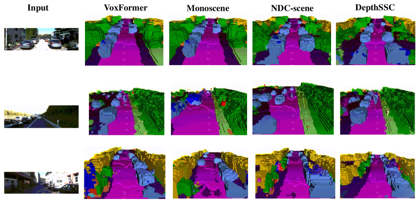
Figure 3: Visualization results against the state-of-the-art monocular SSC method on SemanticKITTI [1] (val set).

4.3 Implementation Details

We utilize 4 NVIDIA 3060 GPUs to train the DepthSSC model across 30 epochs, processing a batch size of 4 images in each iteration. These RGB images are of the resolution 1220×370. During training, we incorporate a random horizontal flip for data augmentation. For optimization, we employ the AdamW optimizer, initiating with a learning rate of 1e-4 coupled with a weight decay of 1e-4. By the time we reach the 5th epoch, we decrease the learning rate by 10%. Both stage-1 and stage-2 are trained separately for 24 epochs, using a learning rate of $2\times 10^{-4}$.

4.4 Main Results

We conducted experiments to evaluate the performance of the DepthSSC on the SemanticKITTI [1] test set and SSCBench-KITTI-360 [12], and compared its results against other state-of-the-art color image-based models.

SemanticKITTI test set.

In Table 1 and 2, the notations Occ, Depth and Pts denote the occupancy grid (3D), depth map (2D) and point cloud (3D), which are the 3D input required by the SSC baselines. For a fair comparison, all the three input are converted from the depth map predicted by a pretrained depth predictor [2].

As shown in Table 1, DepthSSC achieved an IoU of 44.58% and mIoU of 13.11%. In comparison with other models, DepthSSC outperformed all the other methods in terms of IoU, indicating its superior capability in semantic scene completion tasks. In Table 2, on the SemanticKITTI validation set, DepthSSC maintained consistent performance with an IoU of 45.84% and mIoU of 13.28%. Again, it surpassed other models in IoU, showcasing its robustness across different data splits. Examining specific classes, DepthSSC exhibits exceptional competence in recognizing ’building’, ’car’, ’vegetation’, and ’fence’ with scores significantly higher than most other models. However, there are areas for improvement in classes like ’person’ and ’motorcyclist’. While ST-GF aims to align and fuse features accurately, the transformation parameters and clustering mechanisms may not account for the high variability and irregular shapes associated with ’person’ and ’motorcyclist’ classes. These classes often have non-rigid structures that could result in transformations that do not align perfectly with their complex geometries.

Methods	VoxFormer			MonoScene			DepthSSC
Range (m)	12.8m	25.6m	51.2m	12.8m	25.6m	51.2m	12.8m	25.6m	51.2m
IoU (%)	55.45	46.36	38.76	54.65	44.70	37.87	59.37	49.47	40.85
Precision (%)	66.10	61.34	58.52	65.88	59.96	56.73	67.42	63.75	60.69
Recall (%)	77.48	65.48	53.44	76.24	63.72	53.26	77.55	65.96	55.86
mIoU	18.17	15.40	11.91	20.29	16.18	12.31	20.52	17.44	14.28
car (2.85%)	29.41	25.08	17.84	30.83	26.35	19.34	33.72	28.20	21.90
bicycle (0.01%)	2.73	1.73	1.16	1.94	0.83	0.43	1.43	2.85	2.36
motorcycle (0.01%)	1.97	1.47	0.89	3.25	1.30	0.58	5.19	2.15	4.30
truck (0.16%)	6.08	6.63	4.56	14.83	12.18	8.02	16.03	16.03	11.51
other-veh. (5.75%)	3.71	3.56	2.06	6.08	4.30	2.03	6.73	5.13	4.56
person (0.02%)	2.86	2.20	1.63	2.06	1.26	0.86	3.71	1.16	2.92
road (14.98%)	66.10	58.58	47.01	68.60	59.93	48.35	72.28	63.47	50.88
parking (2.31%)	18.44	13.52	9.67	24.32	16.40	11.38	21.72	15.10	12.89
sidewalk (6.43%)	38.00	33.63	27.21	44.43	36.05	28.13	48.79	42.41	30.27
other-grnd(2.05%)	4.49	4.04	2.89	5.76	4.82	3.32	3.87	4.77	2.49
building (15.67%)	41.12	38.24	31.18	45.40	40.60	32.89	46.03	38.65	37.33
fence (0.96%)	8.99	7.43	4.97	9.79	5.91	3.53	10.87	6.81	5.22
vegetation (41.99%)	45.68	35.16	28.99	42.98	32.75	26.15	44.85	39.82	29.61
terrain (7.10%)	24.70	18.53	14.69	31.96	21.63	16.75	25.08	22.13	21.59
pole (0.22%)	8.84	8.16	6.51	9.28	8.45	6.92	10.61	9.15	5.97
traf.-sign (0.06%)	9.15	9.02	6.92	8.58	7.67	5.67	12.98	8.32	7.71
other-struct. (4.33%)	10.31	7.02	3.79	9.18	6.76	4.20	17.18	8.97	5.24
other-obejct (0.28%)	4.40	3.27	2.43	5.86	4.49	3.09	5.53	3.75	3.51

Table 3: Quantitative comparison on SSCBench-KITTI-360 [12]. We present the results for various distance intervals (12.8 meters, 25.6 meters, and 51.2 meters) and furnish metrics for both geometric evaluation (IoU) and semantic assessment (mIoU). The best performance is highlighted in bold.

SSCBench-KITTI-360.

Analyzing the Table 3 results for DepthSSC on the SSCBench-KITTI-360 dataset, it becomes evident that DepthSSC excels particularly in the recognition of roads and sidewalks. This demonstrates DepthSSC’s strong capacity in interpreting and completing scenes involving larger, more contiguous structures. DepthSSC’s comparative advantage over MonoScene in the ’Truck,’ ’Motorcycle,’ and ’Truck’ categories is consistent at different ranges, illustrating DepthSSC’s enhanced dynamic information processing capabilities. At longer ranges, its advantages over the other two benchmark models become more pronounced. This is because DepthSSC can make fuller use of scene geometry information to correct incorrect predictions at a distance.

4.5 Qualitative Visualizations

As shown in Figure 3, there is a visual analysis of scene completion by different models on the SemanticKITTI [1] validation dataset. In the first row, DepthSSC accurately predicts the car ahead, even with severe occlusion present. Meanwhile, other models exhibit varying degrees of missed or misidentified vehicles, often mistaking them for trees or similar objects. In the second column, VoxFormer provides inaccurate shape predictions for the nearby car, predicting only a few grid cells. In contrast, DepthSSC’s predictions for the nearby car are highly accurate, demonstrating excellent shape continuity. In the third row, only the DepthSSC model identifies the pedestrian on the right side, obstructed by a car. This correct prediction necessitates the full utilization of surrounding scene information.

4.6 Ablation Studies

			SemanticKITTI
Methods	w/o GAV	w/o ST-GF	IoU $\uparrow$	mIoU $\uparrow$
Ours	✓	✓	45.84	13.28
Depth-GAV	$\times$	✓	45.25 (-0.59)	13.02 (-0.26)
Depth-ST-GF	✓	$\times$	44.98 (-0.86)	12.87 (-0.41)
VoxFormer [13]	$\times$	$\times$	44.02 (-1.62)	12.35 (-0.93)

Table 4: Components ablation. All of our components boost performance consistently on SemanticKITTI [1].

Analyzing architectural components in DepthSSC.

Using VoxFormer as the baseline model, we introduced the ST-GF (Spatially-Transformed Graph Fusion) module and the GAV (Geometrically-aware Voxelization) module separately, to further validate the effectiveness of DepthSSC, we compare two variants of DepthSSC that are romving GAV and ST-GF, denoted as Depth-GAV and Depth-ST-GF, respectively. Table 4 demonstrates significant improvements from both modules on the VoxFormer model. The ST-GF module ensures accurate alignment of spatial information between the depth map and voxel queries in the 3D scene completion task. By combining spatial transformation and graph structure to optimize feature representation, it effectively enhances VoxFormer’s IoU and mIoU, resulting in improvements of 0.96 and 0.52, respectively, compared to VoxFormer. The GAV module dynamically adjusts voxel resolution by considering the geometric complexity of 3D space, allowing for the capture of more details in geometrically complex regions while conserving computational resources in simpler areas. This adaptive resolution handling enhances VoxFormer’s modeling capability for 3D scenes, leading to improvements in IoU and mIoU by 1.24 and 0.67, respectively.

	Ours(SemanticKITTI)
Alignment Method	IoU $\uparrow$	mIoU $\uparrow$
ST-GF	45.84	13.28
ICP	44.23	12.57
Feature-based Reg.	44.37	12.68
Regularization Matching	44.85	12.94

Table 5: Ablation study for STN in ST-GF module.

ST-GF Ablation Experiments.

The ST-GF module ensures accurate alignment of spatial information between the depth map and voxel queries in the 3D scene completion task by combining spatial transformation and graph structure features. To achieve alignment between the depth map and voxel queries, various spatial transformation or registration techniques can also be employed, including Iterative Closest Point (ICP), feature-based registration, and regularization-based matching methods. Regularization-based matching refers to using optimization techniques to minimize some distance metric between the source and target. Feature-based registration involves first extracting feature points from input data and then using these feature points for matching. As shown in Table 5, the experimental results demonstrate that ST-GF performs the best. However, it’s worth noting that any alignment method can improve the performance of the original VoxFormer.

	Ours(SemanticKITTI)
Distance Metric	IoU $\uparrow$	mIoU $\uparrow$
Euclidean Distance	45.84	13.28
Cosine Similarity	45.37	13.06
Manhattan Distance	45.24	12.89

Table 6: Ablation study on connection strength computation using different distance metrics.

Connection strength Ablation Experiments.

In the ST-GF module, connection strength is used to represent relationships or similarities between different nodes. Connection strength directly affects which relationships are fused in graph convolution computations. This paper compares the performance of semantic scene completion (SSC) under different distance metric methods. Table 6 shows that Euclidean distance achieves the best performance. This is because in three-dimensional space, the actual distance and relative positional relationships between objects are often better captured by Euclidean distance. In contrast, cosine similarity focuses more on direction rather than magnitude, which may not be as suitable for this task. While Manhattan distance also considers spatial aspects, it does not directly account for the shortest distance between two points, which can lead to information loss or inaccuracies in certain cases.

	Ours(SemanticKITTI)
Region-Adaptive Method	IoU $\uparrow$	mIoU $\uparrow$
Resolution-Adaptive Deformable Attention	45.84	13.28
Non-Uniform Voxelization	40.58	10.56
Dynamic Kernel Methods	42.42	11.76
Non-Local Operations	41.39	11.34

Table 7: Ablation study on resolution-adaptive deformable attention.

Resolution-Adaptive Deformable Attention Ablation Experiments.

Resolution-adaptive deformable attention takes into account a core feature of 3D data: different regions may exhibit varying geometric complexities. By designing adaptive resolutions, the model is allowed to have finer voxels in complex regions to capture more details. To validate the superiority of resolution-adaptive deformable attention, comparisons were made with methods such as non-uniform voxelization, dynamic kernel approaches, non-local operations, and axial attention. These methods provide some solutions to address the issue of ”different regions may exhibit varying geometric complexities” to a certain extent. The ablation experiments are presented in Table 7. The experimental results indicate that the mentioned methods all fall short of achieving optimal performance. Non-uniform voxelization may lead to data discontinuities and grid prediction biases. Dynamic kernel methods may encounter alignment issues when dealing with data featuring kernels of different sizes and shapes. Non-local operations require computing relationships between all positions, which can be highly time-consuming in 3D data. While it can capture long-range dependencies, it may not be as effective as deformable attention in capturing local geometric complexities.

5 Conclusion

In this study, we introduced DepthSSC, an advanced single-camera-based semantic scene completion method. It employs spatial transformation and feature fusion techniques to ensure accurate alignment of spatial and depth information. Specifically, through the ST-GF (Spatial Transformation Graph Fusion) module and geometrically-aware voxelization, DepthSSC considers the geometric complexity of 3D space and dynamically adjusts voxel resolutions to adapt to different regions. This approach addresses spatial misalignment and deformation issues present in the state-of-the-art method VoxFormer for monocular semantic scene completion. Through rigorous evaluation on the SemanticKITTI dataset, we demonstrated DepthSSC’s effectiveness in capturing fine details of complex 3D structures, achieving state-of-the-art performance. We anticipate that the DepthSSC approach will inspire further research and advancements in monocular camera-based semantic scene completion.

References

- Behley et al. [2019] Jens Behley, Martin Garbade, Andres Milioto, Jan Quenzel, Sven Behnke, Cyrill Stachniss, and Jurgen Gall. Semantickitti: A dataset for semantic scene understanding of lidar sequences. In Proceedings of the IEEE/CVF international conference on computer vision, pages 9297–9307, 2019.
- Bhat et al. [2021] Shariq Farooq Bhat, Ibraheem Alhashim, and Peter Wonka. Adabins: Depth estimation using adaptive bins. In Proceedings of the IEEE/CVF Conference on Computer Vision and Pattern Recognition, pages 4009–4018, 2021.
- Cao and de Charette [2022] Anh-Quan Cao and Raoul de Charette. Monoscene: Monocular 3d semantic scene completion. In Proceedings of the IEEE/CVF Conference on Computer Vision and Pattern Recognition, pages 3991–4001, 2022.
- Cheng et al. [2021] Ran Cheng, Christopher Agia, Yuan Ren, Xinhai Li, and Liu Bingbing. S3cnet: A sparse semantic scene completion network for lidar point clouds. In Conference on Robot Learning, pages 2148–2161. PMLR, 2021.
- Garbade et al. [2019] Martin Garbade, Yueh-Tung Chen, Johann Sawatzky, and Juergen Gall. Two stream 3d semantic scene completion. In Proceedings of the IEEE/CVF Conference on Computer Vision and Pattern Recognition Workshops, pages 0–0, 2019.
- He et al. [2016] Kaiming He, Xiangyu Zhang, Shaoqing Ren, and Jian Sun. Deep residual learning for image recognition. In Proceedings of the IEEE conference on computer vision and pattern recognition, pages 770–778, 2016.
- Huang et al. [2023] Yuanhui Huang, Wenzhao Zheng, Yunpeng Zhang, Jie Zhou, and Jiwen Lu. Tri-perspective view for vision-based 3d semantic occupancy prediction. In Proceedings of the IEEE/CVF Conference on Computer Vision and Pattern Recognition, pages 9223–9232, 2023.
- Krishna and Murty [1999] K Krishna and M Narasimha Murty. Genetic k-means algorithm. IEEE Transactions on Systems, Man, and Cybernetics, Part B (Cybernetics), 29(3):433–439, 1999.
- Li et al. [2019a] Jie Li, Yu Liu, Dong Gong, Qinfeng Shi, Xia Yuan, Chunxia Zhao, and Ian Reid. Rgbd based dimensional decomposition residual network for 3d semantic scene completion. In Proceedings of the IEEE/CVF Conference on Computer Vision and Pattern Recognition, pages 7693–7702, 2019a.
- Li et al. [2019b] Jie Li, Yu Liu, Xia Yuan, Chunxia Zhao, Roland Siegwart, Ian Reid, and Cesar Cadena. Depth based semantic scene completion with position importance aware loss. IEEE Robotics and Automation Letters, 5(1):219–226, 2019b.
- Li et al. [2020] Jie Li, Kai Han, Peng Wang, Yu Liu, and Xia Yuan. Anisotropic convolutional networks for 3d semantic scene completion. In Proceedings of the IEEE/CVF Conference on Computer Vision and Pattern Recognition, pages 3351–3359, 2020.
- Li et al. [2023a] Yiming Li, Sihang Li, Xinhao Liu, Moonjun Gong, Kenan Li, Nuo Chen, Zijun Wang, Zhiheng Li, Tao Jiang, Fisher Yu, et al. Sscbench: A large-scale 3d semantic scene completion benchmark for autonomous driving. arXiv preprint arXiv:2306.09001, 2023a.
- Li et al. [2023b] Yiming Li, Zhiding Yu, Christopher Choy, Chaowei Xiao, Jose M Alvarez, Sanja Fidler, Chen Feng, and Anima Anandkumar. Voxformer: Sparse voxel transformer for camera-based 3d semantic scene completion. In Proceedings of the IEEE/CVF Conference on Computer Vision and Pattern Recognition, pages 9087–9098, 2023b.
- Li et al. [2022] Zhiqi Li, Wenhai Wang, Hongyang Li, Enze Xie, Chonghao Sima, Tong Lu, Yu Qiao, and Jifeng Dai. Bevformer: Learning bird’s-eye-view representation from multi-camera images via spatiotemporal transformers. In European conference on computer vision, pages 1–18. Springer, 2022.
- Miao et al. [2023] Ruihang Miao, Weizhou Liu, Mingrui Chen, Zheng Gong, Weixin Xu, Chen Hu, and Shuchang Zhou. Occdepth: A depth-aware method for 3d semantic scene completion. arXiv preprint arXiv:2302.13540, 2023.
- Newman and Yi [2006] Timothy S Newman and Hong Yi. A survey of the marching cubes algorithm. Computers & Graphics, 30(5):854–879, 2006.
- Rist et al. [2021] Christoph B Rist, David Emmerichs, Markus Enzweiler, and Dariu M Gavrila. Semantic scene completion using local deep implicit functions on lidar data. IEEE transactions on pattern analysis and machine intelligence, 44(10):7205–7218, 2021.
- Roldao et al. [2020] Luis Roldao, Raoul de Charette, and Anne Verroust-Blondet. Lmscnet: Lightweight multiscale 3d semantic completion. In 2020 International Conference on 3D Vision (3DV), pages 111–119. IEEE, 2020.
- Song et al. [2017] Shuran Song, Fisher Yu, Andy Zeng, Angel X Chang, Manolis Savva, and Thomas Funkhouser. Semantic scene completion from a single depth image. In Proceedings of the IEEE conference on computer vision and pattern recognition, pages 1746–1754, 2017.
- Tian et al. [2023] Xiaoyu Tian, Tao Jiang, Longfei Yun, Yue Wang, Yilun Wang, and Hang Zhao. Occ3d: A large-scale 3d occupancy prediction benchmark for autonomous driving. arXiv preprint arXiv:2304.14365, 2023.
- Wang et al. [2019] Yida Wang, David Joseph Tan, Nassir Navab, and Federico Tombari. Forknet: Multi-branch volumetric semantic completion from a single depth image. In Proceedings of the IEEE/CVF international conference on computer vision, pages 8608–8617, 2019.
- Wei et al. [2023] Yi Wei, Linqing Zhao, Wenzhao Zheng, Zheng Zhu, Jie Zhou, and Jiwen Lu. Surroundocc: Multi-camera 3d occupancy prediction for autonomous driving. In Proceedings of the IEEE/CVF International Conference on Computer Vision, pages 21729–21740, 2023.
- Yan et al. [2021a] Xu Yan, Jiantao Gao, Jie Li, Ruimao Zhang, Zhen Li, Rui Huang, and Shuguang Cui. Sparse single sweep lidar point cloud segmentation via learning contextual shape priors from scene completion. In AAAI, 2021a.
- Yan et al. [2021b] Xu Yan, Jiantao Gao, Jie Li, Ruimao Zhang, Zhen Li, Rui Huang, and Shuguang Cui. Sparse single sweep lidar point cloud segmentation via learning contextual shape priors from scene completion. In Proceedings of the AAAI Conference on Artificial Intelligence, pages 3101–3109, 2021b.
- Yao and Lai [2023] Jiawei Yao and Yingxin Lai. Dynamicbev: Leveraging dynamic queries and temporal context for 3d object detection. arXiv preprint arXiv:2310.05989, 2023.
- Yao et al. [2023a] Jiawei Yao, Chuming Li, Keqiang Sun, Yingjie Cai, Hao Li, Wanli Ouyang, and Hongsheng Li. Ndc-scene: Boost monocular 3d semantic scene completion in normalized device coordinates space. In Proceedings of the IEEE/CVF International Conference on Computer Vision, pages 9455–9465, 2023a.
- Yao et al. [2023b] Jiawei Yao, Chen Wang, Tong Wu, and Chuming Li. Geometry-guided ray augmentation for neural surface reconstruction with sparse views. arXiv preprint arXiv:2310.05483, 2023b.
- Yao et al. [2023c] Jiawei Yao, Tong Wu, and Xiaofeng Zhang. Improving depth gradient continuity in transformers: A comparative study on monocular depth estimation with cnn. arXiv preprint arXiv:2308.08333, 2023c.
- Zhang et al. [2019] Pingping Zhang, Wei Liu, Yinjie Lei, Huchuan Lu, and Xiaoyun Yang. Cascaded context pyramid for full-resolution 3d semantic scene completion. In CVPR, 2019.
- Zhang et al. [2023] Yunpeng Zhang, Zheng Zhu, and Dalong Du. Occformer: Dual-path transformer for vision-based 3d semantic occupancy prediction. arXiv preprint arXiv:2304.05316, 2023.