Broad class of nonlinear Langevin equations with drift and diffusion coefficients separable in time and space: Generalized $n$-moment, ergodicity, Einstein relation and fluctuations of the system

Abstract

A wide class of nonlinear Langevin equations with drift and diffusion coefficients separable in time and space driven by the Gaussian white noise is analyzed in terms of a generalized n-moment. We show the system may present ergodic property, a key property in statistical mechanics, for space-time-dependent drift and diffusion coefficients. A generalized Einstein relation is also obtained. Besides, we show that the first two generalized moments and variance are useful to describe the drift and fluctuations of the system.

I Introduction

Analyses in non-equilibrium statistical systems involve different quantities such as moments and their relations, ergodicity, correlation functions and Einstein relation risken ; kubo ; coffey ; gitter ; snook ; moss ; chers . The probability density function (PDF) is a fundamental quantity from which we can calculate any quantity of interest. In fact, the PDF contains all the information of a system. Non-equilibrium statistical systems have been applied to physics and different interdisciplinary areas coffey ; snook ; moss , for instance, dynamics in graphene-based Josephson junctions spag3 , activation energies of oxygen ion diffusion in yttria stabilized zirconia by flicker noise spectroscopy spag4 , population genetics kimura , spike train statistics for consonant and dissonant musical accords spag5 , a memristor stochastic model spag6 , relativistic Brownian motion dunkel and quantum systems spag8 . In particular, a key property in statistical mechanics is the ergodic property in which the mean-squared displacement (MSD) is equivalent to the time-averaged mean-squared displacement (TAMSD); the practical interest of the ergodic property involves the information obtained from time averages of a single or few trajectories which may represent the ensemble averages. However, many statistical systems exhibit ergodicity breaking; there are only a few systems that present ergodic property. For example, the ergodicity breaking is observed in a Langevin equation with non-constant diffusion coefficients chers and colored noise yong , however diffusion on random fractals presents ergodic property meroz ; meroz2 . Fractional Brownian motion and fractional Langevin equation driven by long-range correlated Gaussian noise are transiently non-ergodic jeon ; jeonB in which time-averaged quantities behave differently from their ensemble-averaged counterparts even for ergodic systems. Ergodicity breaking has also been observed for continuous time random walks model montroll ; montrollB with diverging characteristic waiting time bouch ; bouchB ; bouchC , the blinking dynamics of quantum dots steph , protein motion in human cell walls weig , lipid granule diffusion in yeast cells jeon2 and of insulin granules in MIN6 cells tabei . In fact, these recent investigations have shown ergodicity breaking in most of the systems analyzed. An other interesting quantity is the Einstein relation which connects the first moment in the presence of a constant force to the second moment without any external force, i.e, it connects the fluctuations of an ensemble of particles with their mobility under an applied small load force; it can be obtained from the linear response theory barkai , uncoupled continuous time random walk model barkai ; kwokERc and the Boltzmann transport equation mars . The Einstein relation is also associated with the first fluctuation-dissipation theorem in which the mobility is described in terms of the equilibrium velocity correlation function (using the linear response theory) kubo ; pott . The Einstein relation has been verified by experiments in photocarrier drift and ambipolar diffusion in semiconductors gu and in viscoelastic system amb .

The aim of the work is to consider a wide class of Langevin equations with the drift and diffusion coefficients separable in time and space driven by the Gaussian white noise in the Stratonovich prescription. We investigate the ergodicity, Einstein relation and fluctuations of the system in terms of a generalized $n$-moment. We show that the system may present the ergodic property for space-time-dependent drift and diffusion coefficients, and a generalized Einstein relation may also be obtained. Besides, we show that the first two generalized moments and generalized variance are useful to describe the drift and fluctuations of the system. We also include two systems with time-dependent drift and diffusion coefficients into the discussions.

II Preliminary

We consider the following nonlinear Langevin equation with the drift and diffusion coefficients separable in time and space driven by the Gaussian white noise (in the Stratonovich approach), in one-dimensional space:

$$\frac{dx}{dt}=\left(\beta(t)+\gamma(t)G(x)\right)D(x)+b(t)D(x)L(t),$$ (1)

where $\beta(t)$, $\gamma(t)$ and $b(t)$ are functions of $t$, $D(x)$ is a function of the variable $x$, $G(x)$ is described by

$$\frac{dG(x)}{dx}=\frac{1}{D(x)},$$ (2)

and $L(t)$ is the white noise force with the following averages risken :

$$\left\langle L(t)\right\rangle=0$$ (3)

and

$$\left\langle L(t)L(\overline{t})\right\rangle=2\delta(t-\overline{t}),$$ (4)

where $\delta(z)$ is the Dirac delta function. We also consider $b(t)$ and $D(x)$ non-negative functions. Eq. (1) has been used for various situations such as investigation of turbulent two-particle diffusion in configuration space richar ; richarb ; richarc ; richard ; richare , ergodic property chers ; cher2 ; cher3 ; hou ; cher4 ; leibo ; wang1 ; wang2 , stochastic systems with resetting sandev ; monteiro , stochastic population dynamics calisto2 ; popul ; kwok3 and the fixed samples of the mouse brain using magnetic resonance imaging magin ; kwok4 . It can also describe interesting behaviors such as the asymptotic shape of the random-walk model kwok1 and logarithmic oscillations for the second moment kwok2 . A solution for the PDF and generalized $n$-moment of the above model have been obtained in Ref. kwok2020 . We present below a summary of the results.

The corresponding Fokker-Planck equation for the Langevin equation (1) in the Stratonovich approach is given by risken

$$\frac{\partial\rho(x,t)}{\partial t}=-\frac{\partial}{\partial x}\left[\left(\beta(t)+\gamma(t)G(x)\right)D(x)\rho(x,t)\right]+$$

$$b^{2}(t)\frac{\partial}{\partial x}\left[D(x)\frac{\partial D(x)\rho(x,t)}{\partial x}\right],$$ (5)

where $\rho\left(x,t\right)$ is the PDF.

For solving Eq. (5) we consider the following initial condition kwok2020 :

$$W(G(x),t=0)=\delta\left(G(x)-G_{0}\right),$$ (6)

where $W(x,t)=D(x)\rho(x,t)$ and $G_{0}=G(t=0)$. The PDF has been obtained by using transformations of variables and the Fourier transforms kwok2020 , and it is given by

$$\rho\left(x,t\right)=C\frac{\exp\left[-\frac{\left(G(x)-M(t)\right)^{2}}{2\sigma(t)}\right]}{\sqrt{\sigma(t)}D(x)},$$ (7)

where $C$ is a normalization constant and the coefficients $M\left(t\right)$ and $\sigma\left(t\right)$ are given by

$$M\left(t\right)=G_{0}e^{\int_{0}^{t}\text{d}u\gamma(u)}+\int_{0}^{t}\text{d}z\beta(z)e^{\int_{z}^{t}\text{d}u\gamma(u)}$$ (8)

and

$$\sigma\left(t\right)=2\int_{0}^{t}\text{d}zb^{2}(z)e^{2\int_{z}^{t}\text{d}u\gamma(u)}.$$ (9)

The coefficient $M(t)$ contains only the drift coefficients $\beta(t)$ and $\gamma(t)$. However, the coefficient $\sigma(t)$ contains the diffusion coefficient $b(t)$ and the drift coefficient $\gamma(t)$ due to $G(x)$ in Eq. (1). It can be seen that the coefficient $\sigma(t)$ given by Eq. (9) is a positive quantity.

The PDF (7) can be normalized, however, the interval of the space will depend on the specific system; for example, the variable $x$ in the population growth models is interpreted as the number of population alive at time $t$, which is a non-negative quantity. In particular, the ordinary $n$-moment can be obtained for some specific forms of $D(x)$ kwok2019 . But, we can consider the generalized $n$-moment given by $<G^{n}(x)>$ which recovers the ordinary $n$-moment for $D(x)=1$; in this case we can calculate the generalized $n$-moment for generic $D(x)$. We also consider the whole space (-$\infty$, $\infty$), $\left(G(-\infty)-M(t)\right)/\sqrt{\sigma(t)}\rightarrow-\infty$ and $\left(G(\infty)-M(t)\right)/\sqrt{\sigma(t)}\rightarrow\infty$ with the bounded functions for $M(t)$ and $\sigma(t)$, then the normalized PDF is given by

$$\rho\left(x,t\right)=\frac{\exp\left[-\frac{\left(G(x)-M(t)\right)^{2}}{2\sigma(t)}\right]}{\sqrt{2\pi\sigma(t)}D(x)}.$$ (10)

From the above PDF we can obtain the generalized $n$-moment given by

$$\left<G^{n}(x)\right>=\int_{-\infty}^{\infty}\text{d}xG^{n}(x)\rho\left(x,t\right)=\sqrt{\frac{\left(2\sigma(t)\right)^{n}}{\pi}}\int_{-\infty}^{\infty}\text{d}u\left(u+\frac{M(t)}{\sqrt{2\sigma(t)}}\right)^{n}e^{-u^{2}}$$

$$=\frac{M^{n}(t)}{2\sqrt{\pi}}\sum_{k=0}^{n}\left(\begin{array}[]{c}n\\ k\end{array}\right)\left(\frac{\sqrt{2\sigma(t)}}{M(t)}\right)^{k}\left(1+(-1)^{k}\right)\Gamma\left(\frac{1+k}{2}\right),$$ (11)

where $\Gamma(z)$ is the gamma function.

For instance, the first two generalized moments are given by

$$\left<G(x)\right>=M(t),$$ (12)

and

$$\left<G^{2}(x)\right>=\sigma(t)+M^{2}(t).$$ (13)

The generalized variance can be obtained from the first two generalized moments which yields

$$\left<\left(G(x)-\left<G(x)\right>\right)^{2}\right>=\sigma(t).$$ (14)

Note that the PDF and the generalized $n$-moment can be written in terms of the first generalized moment and generalized variance.

The choice of the observable $G(x)$ in Eq. (11) has various advantages. First we can reduce Eq. (1) to a stochastic system with time-dependent linear force plus a time-dependent load force as follows:

$$\frac{d\bar{x}}{dt}=\beta(t)+\gamma(t)\bar{x}+b(t)L(t),$$ (15)

where $\bar{x}(x)=G(x)$. Moreover, $G(x)$ can be used to obtain the ergodic property of some time-dependent systems described by Eq. (1) for generic $D(x)$, which is in contrast to the observable $x$. The function $G(x)$ can also be used to obtain a generalized Einstein relation. These quantities will be discussed in the next sections.

III Ergodicity

Recently the ergodic property has been investigated in many different systems, and they presented the ergodicity breaking in most of the cases. It is also difficult to find the ergodic property of the system (1) for generic drift and diffusion coefficients. However, the ergodicity of a wide class of systems, with generic diffusion coefficient, may be attained by using the second generalized moment and generalized time average kwokCSF2022 . For the system (1) we can obtain expressions for the generalized correlation function, generalized mean squared displacement (GMSD) and generalized ensemble time average of a single-particle tracking (GETAMSD). As example, we will show that the system (1), with $\beta(t)=\beta$, $\gamma(t)=-\gamma$ and $b(t)=\sqrt{b}$, can present ergodic property by using the GMSD and GETAMSD; this system generalizes the result obtained in Ref. kwokCSF2022 .

The PDF (10) is non-Gaussian due to the non-constant coefficient $D(x)$ and it can describe anomalous diffusion processes kwok2 ; but it is Gaussian for $D(x)=1$. For non-constant $D(x)$ the system can describe different behaviors from those described by $D(x)=1$. For instance, the system (1) for $\beta(t)=\gamma(t)=0$, $b(t)=\sqrt{D}$ and $D(x)=|x|^{\nu/2}$ with $\nu<2$ may present bimodal distribution, and its second moment is given by

$$\left<x^{2}(t)\right>=\frac{\left(D\left(2-\nu\right)^{2}\right)^{\frac{2}{2-\nu}}\Gamma\left(1+\frac{2+\nu}{2(2-\nu)}\right)t^{\frac{2}{2-\nu}}}{\sqrt{\pi}},$$ (16)

where $x_{0}=x(t=0)=0$. Eq. (16) describes subdiffusion ($\nu<0$), normal diffusion ($\nu=0$) and superdiffusion ($\nu>0$) processes, with the ballistic process given by $\nu=1$.

The ergodicity of a system is established by the time average of a single-particle tracking and the MSD which corresponds to an ensemble of particles. The time average of a single-particle tracking (TAMSD) is defined by

$$\overline{\delta^{2}(t)}=\frac{1}{T-t}\int_{0}^{T-t}\left[x\left(\tau+t\right)-x(\tau)\right]^{2}d\tau,$$ (17)

where $t$ is the lag time and $T$ is the measurement time; whereas the MSD is defined by

$$\left<x^{2}(t)\right>=\int_{-\infty}^{\infty}x^{2}\rho\left(x,t\right)dx.$$ (18)

The ergodic property of a system is established when the TAMSD converges to the MSD in the long measurement time limit, i.e, $\lim_{T\rightarrow\infty}\overline{\delta^{2}(t)}=\left<x^{2}(t)\right>$ maria . Usually, we employ the ensemble of $\overline{\delta^{2}(t)}$ which is smoother than $\overline{\delta^{2}(t)}$.

The ergodicity of the system (1) has been investigated in Ref. chers for $\beta(t)=\gamma(t)=0$, $b(t)=\sqrt{D}$, $x_{0}=0$ and $D(x)=|x|^{\nu/2}$ with $\nu<2$, and the result is given by

$$\left<\overline{\delta^{2}(t)}\right>=\left(\frac{t}{T}\right)^{1-p}\left<x^{2}(t)\right>,\ \ t\ll T,$$ (19)

where $p=2/(2-\nu)$ and $\left<\overline{\delta^{2}(t)}\right>$ is the ensemble TAMSD (ETAMSD). The ETAMSD is described by a sum of individual trajectories given by $\left<\overline{\delta^{2}(t)}\right>=N^{-1}\sum_{i=1}^{N}\overline{\delta_{i}^{2}(t)}$, where $N$ is the number of individual trajectories. Eq. (19) shows ergodicity breaking due to the fact that the ETAMSD and the MSD are not equivalent except for the Wiener process ($p=1$); thus the Langevin equation with the space-dependent diffusion coefficient $D(x)=|x|^{\nu/2}$ does not present the ergodic property, in the Stratonovich prescription. The ergodicity breaking is also observed for other functions chers . In general, we will find the ergodicity breaking in the system (1) for non-constant $D(x)$.

However, the ergodic property of the system (1) can be obtained, at least for some class of drift and diffusion coefficients, by using generalizations of the MSD and TAMSD, i.e, we replace the observable $x(t)$ by $G(x)$. In the case of TAMSD, we replace the ordinary squared displacement $\left[x\left(\tau+t\right)-x(\tau)\right]^{2}$ by a generalized squared displacement given by $\left[G\left(\tau+t\right)-G(\tau)\right]^{2}$. In this case, the generalized TAMSD (GTAMSD) is given by

$$\overline{\delta_{G}^{2}(t)}=\frac{1}{T-t}\int_{0}^{T-t}\left[G\left(\tau+t\right)-G(\tau)\right]^{2}d\tau,$$ (20)

where the lower index $G$ on the left-hand side indicates that the ordinary squared displacement is replaced by the generalized squared displacement. The GTAMSD may or may not depend on the initial value $G_{0}$, then the generalized MSD (GMSD) would be chosen according to specific systems in order to attain the ergodic property, i.e., $\left<\left(G(x)-A(t)\right)^{2}\right>$, where $A(t)$ would be chosen according to specific systems; the function $A(t)$ generalizes the initial value $x_{0}$ in the ordinary MSD ($\left<\left(x-x_{0}\right)^{2}\right>$). For systems described below we choose the GMSD as follows:

$$\left<\left(G(x)-G_{0}e^{\int_{0}^{t}\text{d}u\gamma(u)}\right)^{2}\right>=\left<G^{2}(x)\right>-2G_{0}e^{\int_{0}^{t}\text{d}u\gamma(u)}\left<G(x)\right>+G_{0}^{2}e^{2\int_{0}^{t}\text{d}u\gamma(u)}=$$

$$\sigma\left(t\right)+M^{2}(t)-2G_{0}e^{\int_{0}^{t}\text{d}u\gamma(u)}M(t)+G_{0}^{2}e^{2\int_{0}^{t}\text{d}u\gamma(u)}=\sigma\left(t\right)+\bar{M}^{2}(t),$$ (21)

where $A(t)=G_{0}e^{\int_{0}^{t}\text{d}u\gamma(u)}$ and $\bar{M}(t)$ is given by

$$\bar{M}(t)=\int_{0}^{t}\text{d}z\beta(z)e^{\int_{z}^{t}\text{d}u\gamma(u)}.$$ (22)

The difference between $\bar{M}(t)$ and $M(t)$ is that $\bar{M}(t)$ does not contain the initial value $G_{0}$.

It should be noted that the GTAMSD recovers the ordinary TAMSD for $D(x)=1$. In particular, the ergodic property of the system (1) has been verified by using the GTAMSD and GMSD for $\beta(t)=\gamma(t)=0$, $b(t)=\sqrt{D}$ and $D(x)=|x|^{\nu/2}$ with $\nu<2$ kwokCSF2022 .

In order to calculate the GETAMSD for generic $D(x)$, from Eq. (20), we need the generalized correlation function $\left<G(\tau+t)G(\tau))\right>$ which is defined by risken

$$\left<G(t_{2})G(t_{1}))\right>=\int_{-\infty}^{\infty}dx_{2}\int_{-\infty}^{\infty}dx_{1}G\left(x_{2}\right)G\left(x_{1}\right)P(x_{2},t_{2}|x_{1},t_{1})\rho(x_{1},t_{1}),\ \ t_{2}>t_{1},$$ (23)

where $P(x_{2},t_{2}|x_{1},t_{1})$ is the transition probability risken given by

$$P(x_{2},t_{2}|x_{1},t_{1})=\frac{e^{-\frac{\left[G(x_{2})-G(x_{1})e^{\int_{t_{1}}^{t_{2}}du\gamma(u)}-\bar{M}(t_{2},t_{1})\right]^{2}}{2\sigma\left(t_{2},t_{1}\right)}}}{\sqrt{2\pi\sigma\left(t_{2},t_{1}\right)}D(x_{2})},\ \ t_{2}>t_{1},$$ (24)

$$\bar{M}(t_{2},t_{1})=\int_{t_{1}}^{t_{2}}dz\beta\left(z\right)e^{\int_{z}^{t_{2}}du\gamma\left(u\right)}$$ (25)

and

$$\sigma(t_{2},t_{1})=2\int_{t_{1}}^{t_{2}}dzb^{2}\left(z\right)e^{2\int_{z}^{t_{2}}du\gamma\left(u\right)}.$$ (26)

It should be noted that $\bar{M}(t)=\bar{M}(t,0)$ and $\sigma(t)=\sigma(t,0)$. Substituting Eqs. (10) and (24) into Eq. (23) yields

$$\left<G(\tau+t)G(\tau))\right>=e^{\int_{\tau}^{t+\tau}du\gamma\left(u\right)}\left[\sigma\left(\tau,0\right)+\left(G_{0}e^{\int_{0}^{\tau}du\gamma\left(u\right)}+\bar{M}(\tau,0)\right)^{2}\right]+$$

$$\bar{M}(\tau+t,\tau)\left[G_{0}e^{\int_{0}^{\tau}du\gamma\left(u\right)}+\bar{M}(\tau,0)\right].$$ (27)

From Eq. (20) we obtain the following expression for the GETAMSD:

$$\left<\overline{\delta_{G}^{2}(t)}\right>=\frac{1}{T-t}\int_{0}^{T-t}\left[\left<G^{2}\left(\tau+t\right)\right>-2\left<G\left(\tau+t\right)G(\tau)\right>+\left<G^{2}\left(\tau\right)\right>\right]d\tau=$$

$$\frac{1}{T-t}\int_{0}^{T-t}\left\{\sigma\left(\tau+t,0\right)+\left(G_{0}e^{\int_{0}^{\tau+t}du\gamma\left(u\right)}+\bar{M}(\tau+t,0)\right)^{2}-\right.$$

$$\left.2\bar{M}(\tau+t,\tau)\left[G_{0}e^{\int_{0}^{\tau}du\gamma\left(u\right)}+\bar{M}(\tau,0)\right]+\right.$$

$$\left.\left(1-2e^{\int_{\tau}^{\tau+t}du\gamma\left(u\right)}\right)\left[\sigma\left(\tau,0\right)+\left(G_{0}e^{\int_{0}^{\tau}du\gamma\left(u\right)}+\bar{M}(\tau,0)\right)^{2}\right]\right\}d\tau.$$ (28)

Eq. (28) is the GETAMSD for generic $\beta(t)$, $\gamma(t)$ and $b(t)$, which may depend on the initial value $G_{0}$.

Next we take two examples of the generalized correlation function, GMSD and GETAMSD.

Case 1. $\beta(t)=\gamma(t)=0$ and $b(t)=\sqrt{D}$.

This case has been analyzed in Ref. kwokCSF2022 . From Eqs. (21), (27) and (28) we obtain the following generalized correlation function, GMSD and GETAMSD:

$$\left<G(\tau+t)G(\tau))\right>=2D\tau+G_{0}^{2},$$ (29)

$$\left<\left(G(x)-G_{0}\right)^{2}\right>=2Dt$$ (30)

and

$$\left<\overline{\delta_{G}^{2}(t)}\right>=2Dt.$$ (31)

Eq. (31) shows that the GETAMSD does not depend on the initial value $G_{0}$. We can see that the GMSD and GETAMSD given by Eqs. (30) and (31) scale linearly and they also recover the results of the Wiener process for $D(x)=1$. Comparing Eq. (30) with Eq. (31) yields

$$\left<\overline{\delta_{G}^{2}(t)}\right>=2Dt=\left<\left(G(x)-G_{0}\right)^{2}\right>.$$ (32)

Eq. (32) shows that the ergodicity is attained for the system (1) by using modified MSD and TAMSD.

Case 2. $\beta(t)=\beta$, $\gamma(t)=-\gamma$ and $b(t)=\sqrt{b}$.

In this case the generalized correlation function, GMSD and GETAMSD are described by

$$\left<G(\tau+t)G(\tau))\right>=e^{-\gamma t}\left[\frac{b}{\gamma}\left(1-e^{-2\gamma\tau}\right)+\left(G_{0}e^{-\gamma\tau}+\frac{\beta}{\gamma}\left(1-e^{-\gamma\tau}\right)\right)^{2}\right]+$$

$$\frac{\beta}{\gamma}\left(1-e^{-\gamma t}\right)\left(G_{0}e^{-\gamma\tau}+\frac{\beta}{\gamma}\left(1-e^{-\gamma\tau}\right)\right),$$ (33)

$$\left<\left(G(x)-G_{0}e^{-\gamma t}\right)^{2}\right>=\frac{b}{\gamma}\left(1-e^{-2\gamma t}\right)+\frac{\beta^{2}}{\gamma^{2}}\left(1-e^{-\gamma t}\right)^{2}$$ (34)

and

$$\left<\overline{\delta_{G}^{2}(t)}\right>=\frac{2b}{\gamma}\left(1-e^{-\gamma t}\right)+\frac{1}{T-t}\left[\frac{b}{2\gamma^{2}}-\frac{\left(G_{0}-\frac{\beta}{\gamma}\right)^{2}}{2\gamma}\right]\left(1-e^{-\gamma t}\right)^{2}\left(e^{-2\gamma(T-t)}-1\right).$$ (35)

The expressions for the GMSD and GETAMSD are very different and, consequently, the system does not present the ergodic property for generic parameter values. Moreover, the GETAMSD given by Eq. (35) depends explicitly on the initial value $G_{0}$ and the measurement time T, except the first term on the right-hand side. The ergodic property can be obtained from Eqs. (34) and (35) by taking $\beta=0$ and $\gamma\rightarrow 0$. For $D(x)=1$ the system recovers the Ornstein-Uhlenbeck process with the presence of a load force. The results (34) and (35) for $D(x)=1$, $\beta=0$ and $x_{0}=0$ are in agreement with those presented in Ref. jeon3 . It should be noted that the ergodic property of the Wiener process is obtained from Eqs. (34) and (35) by taking $D(x)=1$, $\beta=0$ and $\gamma\rightarrow 0$.

It can be seen that, from Eqs. (34) and (35), the GMSD and GETAMSD present plateaus due to the term $G(x)$ in Eq. (1). It is interesting to note that $\beta$ does not generate a new term in Eq. (35), but it is associated with the constants $b$ and $G_{0}$ which is in contrast to the result of the GMSD. Moreover, from Eqs. (34) and (35), the system presents ergodicity breaking for $\beta=0$ and $\gamma\neq 0$. Figs. (1) and (2) show the simulated and analytical results for the GETAMSD with different parameter values and $x_{0}\neq 0$. The analytical and theoretical results are in good agreement, and they do not depend on the $D(x)$. For comparison we have taken $x_{0}=1$ for Fig. (1) and $G_{0}=10$ for Fig. (2). They show the behaviors of the GETAMSD which depend on the initial values. The curve in the bottom of Fig. (1) has the behavior changed by the initial value which is shown in Fig. (2).

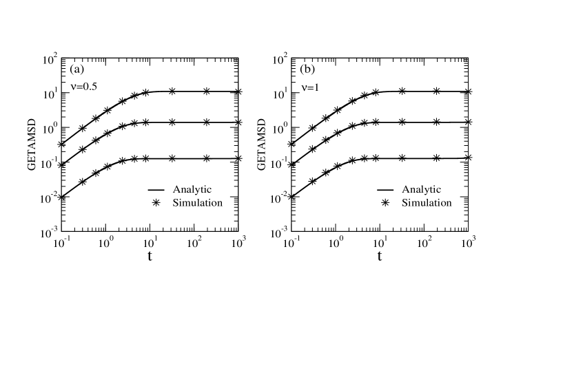
Figure 1: Log-log plots of the simulated and analytical results for the GETAMSD with $D(x)=|x|^{\nu/2}$. The analytical result is described by Eq. (35). We take the initial value $x_{0}=1$ and $T=1200$. The parameter values ($\beta$, $\gamma$ and $b$) are the same for both figures ((a) and (b)); from top to bottom the parameter values are: $\beta=0.7$, $\gamma=0.3$, $b=\beta^{2}/\gamma=1.6333$; $\beta=-0.5$, $\gamma=0.6$, $b=\beta^{2}/\gamma=.4167$; $\beta=0.2$, $\gamma=0.8$, $b=\beta^{2}/\gamma=0.05$. In a) the parameter $\nu$ is given by $\nu=1/2$, and $\nu=1$ for b).

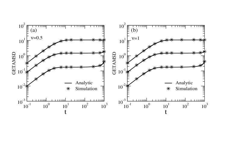
Figure 2: Log-log plots of the simulated and analytical results for the GETAMSD with $D(x)=|x|^{\nu/2}$. The analytical result is described by Eq. (35). We take the initial value $G_{0}=10$ and $T=1200$. The parameter values ($\beta$, $\gamma$ and $b$) are the same for both figures ((a) and (b)); from top to bottom the parameter values are: $\beta=0.7$, $\gamma=0.3$, $b=\beta^{2}/\gamma=1.6333$; $\beta=-0.5$, $\gamma=0.6$, $b=\beta^{2}/\gamma=.4167$; $\beta=0.2$, $\gamma=0.8$, $b=\beta^{2}/\gamma=0.05$. In a) the parameter $\nu$ is given by $\nu=1/2$, and $\nu=1$ for b).

For $t\ll 1$ and $T\gg t$ Eq. (35) is given by

$$\left<\overline{\delta_{G}^{2}(t)}\right>\approx\left<\left(G(x)-G_{0}e^{-\gamma t}\right)^{2}\right>+\frac{1}{\gamma}\left(b-\frac{\beta^{2}}{\gamma}\right)\left(1-e^{-\gamma t}\right)^{2}.$$ (36)

From Eq. (36) we can obtain the ergodic property for $t\ll 1$ and $T\gg t$ and $b=\beta^{2}/\gamma$.

For $t\approx T$ Eq. (35) is given by

$$\left<\overline{\delta_{G}^{2}(t)}\right>\approx\frac{2b}{\gamma}\left(1-e^{-\gamma t}\right)+\left[\left(G_{0}-\frac{\beta}{\gamma}\right)^{2}-\frac{b}{\gamma}\right]\times$$

$$\left(1-e^{-\gamma t}\right)^{2}\left[1-\gamma(T-t)\right].$$ (37)

Eq. (37) can be written in terms of $\left<(G(x)-G_{0}e^{-\gamma t})^{2}\right>$ as follows:

$$\left<\overline{\delta_{G}^{2}(t)}\right>\approx\left<\left(G(x)-G_{0}e^{-\gamma t}\right)^{2}\right>+\frac{1}{2\gamma}\left(G_{0}^{2}-\frac{2G_{0}\beta}{\gamma}\right)\left(1-e^{-\gamma t}\right)^{2}-$$

$$\gamma\left[\left(G_{0}-\frac{\beta}{\gamma}\right)^{2}-\frac{b}{\gamma}\right](T-t)\left(1-e^{-\gamma t}\right)^{2}.$$ (38)

Eq. (38) shows that the ergodic property can be obtained from $G_{0}\neq 0$ with additional conditions $G_{0}=2\beta/\gamma$ and $b=\beta^{2}/\gamma$. Moreover, the GETAMSD converges to the GMSD for $b=\beta^{2}/\gamma$ and $G_{0}=0$, i.e,

$$\left<G^{2}(x)\right>=\left<\overline{\delta_{G}^{2}(t)}\right>.$$ (39)

For $D(x)=1$ the system describes the ergodicity of the Ornstein-Uhlenbeck process restored by a load force.

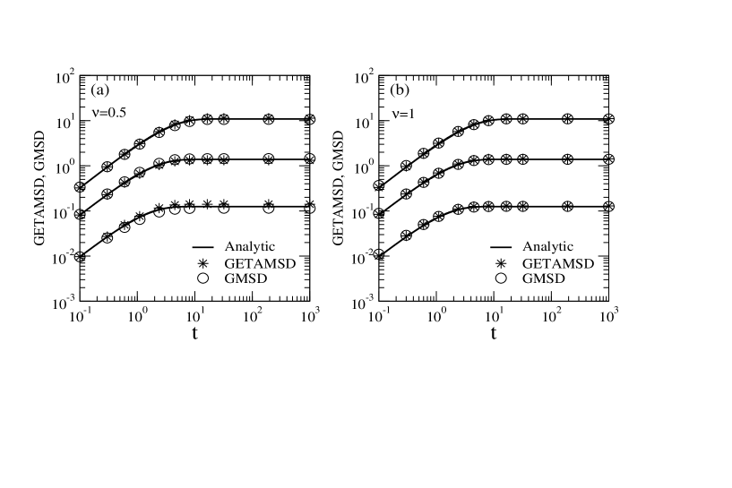
Figure 3: Log-log plots of the simulated and analytical results for the GMSD and GETAMSD with $D(x)=|x|^{\nu/2}$. The analytical result is described by Eq. (40). We take the initial value $x_{0}=0$ and $T=1200$. The parameter values ($\beta$, $\gamma$ and $b$) are the same for both figures ((a) and (b)); from top to bottom the parameter values are: $\beta=0.7$, $\gamma=0.3$, $b=\beta^{2}/\gamma=1.6333$; $\beta=-0.5$, $\gamma=0.6$, $b=\beta^{2}/\gamma=.4167$; $\beta=0.2$, $\gamma=0.8$, $b=\beta^{2}/\gamma=0.05$. In a) the parameter $\nu$ is given by $\nu=1/2$, and $\nu=1$ for b).

The above behaviors for $D(x)=1$ are the same for generic $D(x)$ when we use the generalized moments. In fact, the ergodic property of the system can be attained by taking $G_{0}=0$ and $\beta^{2}/\gamma=b$ or $T-t\gg 1$ and $\beta^{2}/\gamma=b$, and we have

$$\left<\overline{\delta_{G}^{2}(t)}\right>=\frac{2b}{\gamma}\left(1-e^{-\gamma t}\right)=\left<\left(G(x)+G_{0}e^{-\gamma t}\right)^{2}\right>.$$ (40)

It should be noted that the above ergodic property is valid for $G_{0}\neq 0$, with the conditions $T-t\gg 1$ and $\beta^{2}/\gamma=b$. Eq. (40) shows that the ergodic property is attained for the system (1) with generic $D(x)$ by using generalized MSD and TAMSD. The expression (40) presents plateau, given by $2b/\gamma$, for $\gamma t\gg 1$, due to $G(x)$ in Eq. (1). The plateau disappears for $\gamma\rightarrow 0$ and the expression (40) reduces to

$$\left<\overline{\delta_{G}^{2}(t)}\right>=2bt=\left<\left(G(x)-G_{0}\right)^{2}\right>,$$ (41)

which has the same result of the first case.

Fig. 3 shows the behaviors of the GMSD and GETAMSD for $D(x)$ described by a power-law; they present ergodic property with $b=\beta^{2}/\gamma$. Figs. 3a and 3b show behaviors for the same parameter values ($\beta$, $\gamma$ and $b$), but with different values of $\nu$. We can see the behaviors are independent of $D(x)$. Moreover, the simulations are in very good agreement with the analytical results.

IV Generalized variance, fluctuations and generalized Einstein relation

Fluctuations represent an important part of a stochastic system. However, in many cases the fluctuations are not easily identified and calculated. For systems driven by multiplicative noise the fluctuations can not be separated from the drift using the first two moments due to the connection between the dependent variable and the noise. For example, we consider $D(x)=x$ from which the space is limited to $0<x<\infty$ due to the normalization of the PDF; this system presents interesting results in which the moments can be related among them. The coefficient $D(x)=x$ may also be useful to describe population growth models (see, for instance, roman ). In this case, the $n$-moment can be calculated exactly. From the PDF (7) we obtain

$$\left<x^{n}\right>=e^{nM(t)+\frac{n^{2}\sigma(t)}{2}}.$$ (42)

We can see that the time-dependent drift and diffusion coefficients in the $n$-moment can not be separated as a sum due to the exponential function. Therefore, we can not obtain a quantity related to the fluctuations of the system by using the ordinary $n$-moment and variance. In order to separate $\sigma(t)$ from $M(t)$ we have to consider the following expressions:

$$\frac{\left<x^{2n}\right>}{\left<x^{n}\right>^{2}}=e^{n^{2}\sigma(t)}$$ (43)

and

$$\frac{\left<x^{n}\right>^{4}}{\left<x^{2n}\right>}=e^{2nM(t)}.$$ (44)

We can see that Eq. (43) contains $n$ relations which depend only on the coefficient $\sigma(t)$, whereas Eq. (44) contains $n$ relations which depend only on the time-dependent drift coefficients. For $n=1$ Eqs. (43) and (44) reduce to

$$\frac{\left<x^{2}\right>}{\left<x\right>^{2}}=e^{\sigma(t)}$$ (45)

and

$$\frac{\left<x\right>^{4}}{\left<x^{2}\right>}=e^{2M(t)}.$$ (46)

Eqs. (45) and (46) are relations which contain only the first two moments. They can be written in terms of the relations (43) and (44) as follows:

$$\frac{\left<x^{2n}\right>}{\left<x^{n}\right>^{2}}=\left(\frac{\left<x^{2}\right>}{\left<x\right>^{2}}\right)^{n^{2}}$$ (47)

and

$$\frac{\left<x^{n}\right>^{4}}{\left<x^{2n}\right>}=\left(\frac{\left<x\right>^{4}}{\left<x^{2}\right>}\right)^{n}.$$ (48)

Besides, we can obtain the following relation by using Eqs. (47) and (48):

$$\left<x^{n}\right>^{2}=\left<x^{2}\right>^{n(n-1)}\left<x\right>^{2n(2-n)}.$$ (49)

Eqs. (47), (48) and (49) show that the quantities $\left<x^{2n}\right>/\left<x^{n}\right>^{2}$, $\left<x^{n}\right>^{4}/\left<x^{2n}\right>$ and $\left<x^{n}\right>^{2}$ can be factorized in terms of the first two moments.

For $\gamma(t)=0$ Eq. (43) reduces to

$$\frac{\left<x^{2n}\right>}{\left<x^{n}\right>^{2}}=e^{2n^{2}\int_{0}^{t}\text{d}zb^{2}(z)},$$ (50)

which depends only on the time-dependent diffusion coefficient $b(t)$. However, we can use the first generalized moment and generalized variance to quantify the drift and fluctuations of the system,

$$\left<G(x)\right>=M(t)$$ (51)

and

$$\left<\left(G(x)-\left<G(x)\right>\right)^{2}\right>=\sigma(t).$$ (52)

The coefficient $\sigma(t)$ contains $\gamma(t)$ due to $G(x)$ in Eq. (1). In order to obtain a quantity which depends only on the time-dependent diffusion coefficient we should take $\gamma(t)=0$. Then, the first generalized moment describes only the deterministic part of the system, whereas the generalized variance is related to the fluctuations of the system. Fig. 4 shows the simulated and analytical results for the relation (45) and the generalized variance described by Eq. (52); they are in good agreement. The plateaus are due to $G(x)$ in Eq. (1).

It is interesting to note that the ordinary $n$-moment can be written in terms of the first generalized moment and generalized variance as follows:

$$\left<x^{n}\right>=e^{n\left<G(x)\right>+\frac{n^{2}\left<\left(G(x)-\left<G(x)\right>\right)^{2}\right>}{2}}.$$ (53)

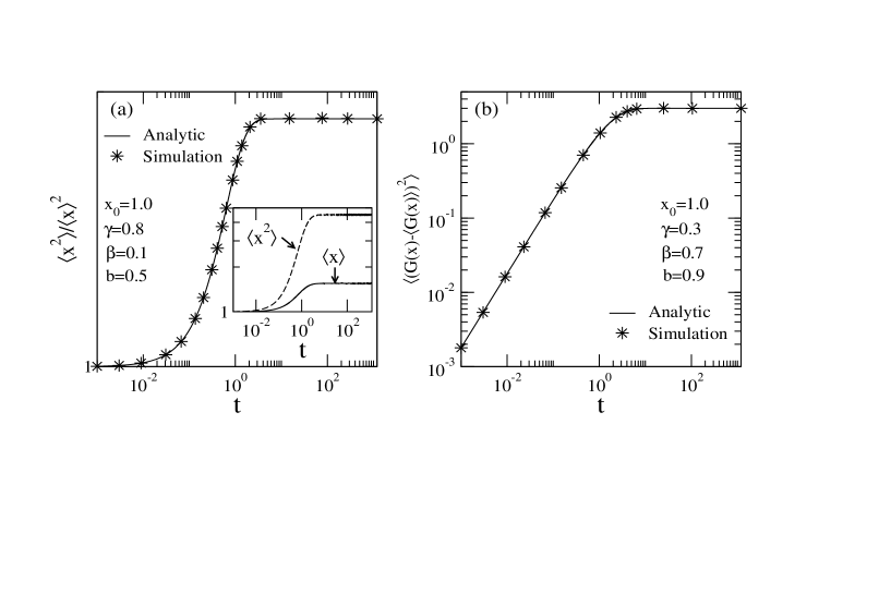
Figure 4: Log-log plots of the simulated and analytical results for the relation (45) and the generalized variance described by Eq. (52). The time-dependent coefficients are given by $\beta(t)=\beta$, $\gamma(t)=-\gamma$ and $b(t)=\sqrt{b}$.

Now we consider two applications of the Langevin equation (1) with non-constant coefficients. In the first one we take the application of the generalized variance for a reformulation of the Verhulst logistic diffusion model described in Ref. roman by using the time-space-dependent drift coefficient as follows:

$$\frac{dx}{dt}=\frac{bc}{b+e^{ct}}x+\bar{\sigma}xL(t),\ \ 0<x<\infty.$$ (54)

Eq. (54) is a Langevin equation in the Ito prescription which has been used to describe a culture of microorganisms roman . However, the solution (7) has been obtained in the Stratonovich prescription. The corresponding Langevin equation (1) to the Ito prescription is given by

$$\frac{dx}{dt}=b\left(\frac{c}{b+e^{ct}}-\frac{\bar{\sigma}^{2}}{b}\right)x+\bar{\sigma}xL(t),$$ (55)

which has an additional term in the drift term.

In this case, the drift and diffusion coefficients of Eq. (1) are given by $b(t)=\bar{\sigma}$, $\beta(t)=bc/\left(b+e^{ct}\right)-\bar{\sigma}^{2}$, $\gamma(t)=0$ and $D(x)=x$. The normalization of the PDF implies that $x$ should also be restricted to $0<x<\infty$ and we obtain

$$\rho\left(x,t\right)=\frac{e^{-\frac{\left(\ln\left(\frac{x}{x_{0}}\right)-\left(c-\bar{\sigma}^{2}\right)t-\ln\left(\frac{1+b}{b+e^{ct}}\right)\right)^{2}}{4\bar{\sigma}^{2}t}}}{\sqrt{4\pi\bar{\sigma}^{2}t}x}.$$ (56)

The ordinary $n$-moment can be calculated from Eq. (42) and it is given by

$$\left<x^{n}\right>=\left[\frac{x_{0}(1+b)}{1+be^{-ct}}\right]^{n}e^{-n(1-n)\bar{\sigma}^{2}t}.$$ (57)

For the first moment we have

$$\left<x\right>=\frac{x_{0}(1+b)}{1+be^{-ct}}.$$ (58)

Eq. (58) has the same result reported in Ref. roman . We can see that the first moment (58) does not depend on the parameter $\bar{\sigma}$ due to the fact that the drift coefficient has the term (-$\bar{\sigma}^{2}x$) which cancels the spurious drift term generated from the Stratonovich prescription. A quantity related to the diffusion coefficient can be described by Eq. (50),

$$\frac{\left<x^{2}\right>}{\left<x\right>^{2}}=e^{2\bar{\sigma}^{2}t}.$$ (59)

We can quantify the fluctuations of the noise by using the generalized variance given by

$$\left<\left(\ln(x)-\left<\ln(x)\right>\right)^{2}\right>=2\bar{\sigma}^{2}t.$$ (60)

It can be seen that the generalized variance has a more simple form to quantify the noise than the expression (59).

The second application of the system (1) is on the impact of chloride ion diffusion in concrete liu ; yan . The studies indicated that chloride ion diffusion in concrete is time-dependent yan . The model used in Ref. yan is, basically, a diffusion equation with time-dependent diffusion coefficient described by

$$\frac{\partial\rho(x,t)}{\partial t}=Db_{\eta}t^{\eta}\frac{\partial^{2}\rho(x,t)}{\partial x^{2}},$$ (61)

where $\rho(x,t)$ describes the concentration of the chloride ions. The model (61) can be described in terms of the Langevin equation (1) with $\beta=\gamma=0$, $D(x)=1$ and $b(t)=Db_{\eta}t^{\eta}$.

IV.1 Generalized Einstein relation

A connection between the fluctuations of an ensemble of particles and their mobility under an applied small load force is described by the second Einstein relation which connects the first moment in the presence of a constant force to the second moment without any external force. In this case, the PDF is described by a Gaussian distribution. The Einstein relation has been generalized for the cases of non-Gaussian distributions described by a wide class of non-linear Langevin equations kwokERc . Now we generalize the Einstein relation to the system (1). We first consider the first generalized moment given by Eq. (12). Then we connect the first generalized moment to the generalized variance (52) as follows:

$$\left<\left(G(x)-G_{0}e^{\int_{0}^{t}\text{d}u\gamma(u)}\right)\right>=\left<\left(G(x)-\left<G(x)\right>\right)^{2}\right>$$ (62)

by taking

$$\int_{0}^{t}\text{d}z\beta(z)e^{\int_{z}^{t}\text{d}u\gamma(u)}=2\int_{0}^{t}\text{d}zb^{2}(z)e^{2\int_{z}^{t}\text{d}u\gamma(u)}.$$ (63)

As example, we take $\beta(t)=b^{2}(1+e^{2\gamma t})$, $\gamma(t)=\gamma$ and $b(t)=b$; they satisfy the relations (62) and (63).

However, for the generalized variance (52) to describe only the fluctuations of the noise we should take $\gamma(t)=0$, then we have

$$\int_{0}^{t}\text{d}z\beta(z)e^{\int_{z}^{t}\text{d}u\gamma(u)}=2\int_{0}^{t}\text{d}zb^{2}(z),$$ (64)

and the generalized second Einstein relation for the system (1) is described by

$$\left<\left(G(x)-G_{0}e^{\int_{0}^{t}\text{d}u\gamma(u)}\right)\right>_{\gamma}=\left<\left(G(x)-\left<G(x)\right>\right)^{2}\right>_{\gamma=0}.$$ (65)

As example, we take $\beta(t)=2b^{2}(1-\gamma t)$, $\gamma(t)=\gamma$ and $b(t)=b$; they satisfy the relations (64) and (65).

V Conclusion

A wide class of nonlinear Langevin equations with the drift and diffusion coefficients separable in time and space has been considered, and they can be applied to various systems. We have obtained solutions for the generalized correlation function (27) and GETAMSD (28). As is well-known, the Langevin equation with space-time-dependent coefficients may describe complicated behaviors, then a convenient choice of the observable may be useful to simplify the results of $n$-moment and also lead to some new relations and properties. We have shown that the observable $G(x)$ is useful to describe the system (1) with space-time-dependent drift and diffusion coefficients in the Stratonovich prescription: It can be used to obtain a generalized Einstein relation and attain ergodicity, and it is also useful to calculate the mean generalized squared displacement of the fluctuations of the system by using the generalized variance. A new relation which connects the ordinary $n$-moment with the first two generalized moments has also been obtained (53).

Possibly, as an extension of this work, we may also use the observable $G(x)$ or other generalized observables to calculate generalized moments of more complicated systems described by

$$\frac{dx}{dt}=h(x,t)+g(x,t)L(t),$$ (66)

where $h(x,t)$ and $g(x,t)$ are some class of generic functions which depend on the space-time coordinates. See Ref. kwokAsym for a system different from Eq. (1) in which the observable $G(x)$ has been employed for calculating the generalized $n$-moment.

References

- (1) Risken H 1996 The Fokker–Planck Equation 2nd edn (Berlin: Springer-Verlag)
- (2) Kubo R, Toda M and Hashitsume N 1985 Statistical Physics II. Nonequilibrium Statistical Mechanics (Germany: Springer)
- (3) Coffey W T and Kalmykov Y P 2017 The Langevin Equation: With Applications To Stochastic Problems in Physics, Chemistry, and Electrical Engineering fourth edn (New Jersey: World Scientific)
- (4) Gitterman M 2005 The Noisy Oscillator (Singapore: World Scientific)
- (5) Snook I 2007 The Langevin and Generalised Langevin Approach To the Dynamics of Atomic, Polymeric and Colloidal Systems (Netherlands: Elsevier)
- (6) Moss F and McClintock PVE (editors) 1989 Noise in Nonlinear Dynamical Systems Vols. 1–3 (Cambridge: Cambridge University Press)
- (7) Cherstvy A G, Chechkin A V and Metzler R 2013 New. J. Phys. 15 083039
- (8) Guarcello C, Valenti D, Spagnolo B, Pierro V and Filatrella G 2017 Nanotechnology 28 134001
- (9) Yakimov A V, Filatov D O, Gorshkov O N, Antonov D A, Liskin D A, Antonov I N, Belyakov A V, Klyuev A V, Carollo A and Spagnolo B 2019 Appl. Phys. Lett. 114 253506
- (10) Kimura M 1964 J. Appl. Probab. 1 177
- (11) Ushakov Y V, Dubkov A A and Spagnolo B 2010 Phys. Rev. E 81 041911
- (12) Agudov N V, Safonov A V, Krichigin A V, Kharcheva A A, Dubkov A A, Valenti D, Guseinov D V, Belov A I, Mikhaylov A N, Carollo A and Spagnolo B 2020 J. Stat. Mech. 024003
- (13) Dunkel J and Hanggi P 2009 Phys. Rep. 471 1
- (14) Carollo A, Spagnolo B, Dubkov A A and Valenti D 2019 J. Stat. Mech. 094010
- (15) Xu Y, Liu X M, Li Y G and Metzler R 2020 Phys. Rev. E 102 062106
- (16) Meroz Y, Eliazar I and Klafter J 2009 J. Phys. A: Math. Theor. 42 434012
- (17) Meroz Y, Sokolov I M and Klafter J 2013 Phys. Rev. Lett. 110 090601
- (18) Deng W H and Barkai E 2009 Phys. Rev. E 79 011112
- (19) Jeon J H, Leijnse N, Oddershede L B and Metzler R 2013 New J. Phys. 15 045011
- (20) Montroll E W and Weiss G H 1965 J. Math. Phys. 6 167
- (21) Scher H and Montroll E W 1975 Phys. Rev. B 12 2455
- (22) Bouchaud J P 1992 J. Physique I 2 1705
- (23) Bel G and Barkai E 2005 Phys. Rev. Lett. 94 240602
- (24) Rebenshtok A and Barkai E 2007 Phys. Rev. Lett. 99 210601
- (25) Stefani F D, Hoogenboom J P and Barkai E 2009 Phys. Today 62 34
- (26) Weigel A V, Simon B, Tamkun M M and Krapf D 2011 Proc. Natl. Acad. Sci. USA 108 6438
- (27) Jeon J H, Tejedor V, Burov S, Barkai E, Selhuber-Unkel C, Berg-Sorensen K, Oddershede L and Metzler R 2011 Phys. Rev. Lett. 106 048103
- (28) Tabei S M A, Burov S, Kim H Y, Kuznetsov A, Huynh T, Jureller J, Philipson L H, Dinner A R and Scherer N F 2013 Proc. Natl. Acad. Sci. USA 110 4911
- (29) Barkai E and Fleurov V N 1998 Phys. Rev. E 58 1296
- (30) Fa K S, Pianegonda S and da Luz M G E 2023 Physica A 622 128807
- (31) Marshak A H and Assaf D 1973 Solid-State Elect. 16 675
- (32) Pottier N 2005 Physica A 345 472
- (33) Gu Q, Schiff E A, Grebner S, Wang F and Schwarz R 1996 Phys. Rev. Lett. 76 3196
- (34) Amblard F, Maggs A C, Yurke B, Pargellis A N and Leibler S 1996 Phys. Rev. Lett. 77 4470
- (35) Richardson L F 1926 Proc. R. Soc. London, Ser. A 110 709
- (36) Kolmogorov A N 1941 Dokl. Acad. Sci. URSS 30 301
- (37) Batchelor G K 1952 Proc. Cambridge Philos. Soc. 48 345
- (38) Okubo A 1962 J. Oceanogr. Soc. Jpn. 20 286
- (39) Hentschel H G E and Procaccia I 1984 Phys. Rev. A 29 1461
- (40) Cherstvy A G, Chechkin A V and Metzler R 2014 J. Phys. A: Math. Theor. 47 485002
- (41) Cherstvy A G and Metzler R 2015 J. Stat. Mech. P05010.
- (42) Hou R, Cherstvy A G, Metzler R and Akimoto T 2018 Phys. Chem. Chem. Phys. 20 20827
- (43) Cherstvy A G, Thapa S, Mardoukhi Y, Chechkin A V and Metzler R 2018 Phys. Rev. E 98 022134
- (44) Leibovich N and Barkai E 2019 Phys. Rev. E 99 042138
- (45) Wang W, Cherstvy A G, Liu X B and Metzler R 2020 Phys. Rev. E 102 012146
- (46) Vinod D, Cherstvy A G, Wang W, Metzler R and Sokolov I M 2022 Phys. Rev. E 105 L012106
- (47) Sandev T, Domazetoski V, Kocarev L, Metzler R and Chechkin A 2022 J. Phys. A: Math. and Theor. 55 074003
- (48) Montero M, Perelló J and Masoliver J 2022 J. Phys. A: Math. and Theor. 55 464001
- (49) Aquino G, Bologna M and Calisto H 2010 EPL 89 50012
- (50) Jackson P J, Lambert C J, Mannella R, Martano P, McClintock P V E and Stocks N G 1989 Phys. Rev. A 40 2875
- (51) Fa K S 2012 Annals Phys. 327 1989
- (52) Liang Y J, Ye A Q, Chen W, Gatto R G, Colon-Perez L, Mareci T H and Magin R L 2016 Commun. Nonlinear Sci. Numer. Simul. 39 529
- (53) Fa K S 2017 J. Stat. Mech. 033207.
- (54) Fa K S 2005 Phys. Rev. E 72 020101
- (55) Fa K S 2011 Phys. Rev. E 84 012102
- (56) Fa K S 2020 J. Stat. Mech. 093206.
- (57) Fa K S 2019 J. Stat. Mech. 063205.
- (58) Fa K S 2022 Chaos, solitons and fractals 160 112263
- (59) Schwarzl M, Godec A and Metzler R 2017 Sci. Rep. 7 3878
- (60) Jeon J H and Metzler R 2012 Phys. Rev. E 85 021147
- (61) Román-Román P and Torres-Ruiz F 2012 Biosys. 110 9
- (62) QU P F, Liu X T and Baleanu D 2019 Thermal Sci. 23 S67
- (63) Yan S J and Liang Y J 2023 J. Building Eng. 74 106897
- (64) Fa K S, Ho C L, Matos Y B and da Luz M G E 2023 Phys. Scr. 98 115001