Efficient Deep Speech Understanding at the Edge

Abstract.

In contemporary speech understanding (SU), a sophisticated pipeline is employed, encompassing the ingestion of streaming voice input. The pipeline executes beam search iteratively, invoking a deep neural network to generate tentative outputs (referred to as hypotheses) in an autoregressive manner. Periodically, the pipeline assesses attention and Connectionist Temporal Classification (CTC) scores.

This paper aims to enhance SU performance on edge devices with limited resources. Adopting a hybrid strategy, our approach focuses on accelerating on-device execution and offloading inputs surpassing the device’s capacity. While this approach is established, we tackle SU’s distinctive challenges through innovative techniques: Late Contextualization: This involves the parallel execution of a model’s attentive encoder during input ingestion. Pilot Inference: Addressing temporal load imbalances in the SU pipeline, this technique aims to mitigate them effectively. Autoregression Offramps: Decisions regarding offloading are made solely based on hypotheses, presenting a novel approach.

These techniques are designed to seamlessly integrate with existing speech models, pipelines, and frameworks, offering flexibility for independent or combined application. Collectively, they form a hybrid solution for edge SU. Our prototype, named XYZ, has undergone testing on Arm platforms featuring 6 to 8 cores, demonstrating state-of-the-art accuracy. Notably, it achieves a 2x reduction in end-to-end latency and a corresponding 2x decrease in offloading requirements.

1. Introduction

Speech is a pervasive user interface for embedded devices. At its core are two speech understanding (SU) tasks: automatic speech recognition (ASR) transcribes voice to a sentence (yu2016automatic, ); spoken language understanding (SLU) maps voice to a structured intent, such as {scenario: Calendar, action: Create_entry} (de2007spoken, ).

Modern SU: autoregression with beam search

Modern SU runs a deep, encoder-decoder model (Jan2015NIPS, ) as shown in Figure 1. Ingesting an utterance waveform, the model comprises a neural encoder, which captures dependency among sound units, and a neural decoder, which generates a sequence of tokens as words or sub-words. This generation process is autoregressive: to produce a token, the decoder takes as the input all the latent units produced by the encoder, as well the output tokens it produces so far. To cope with noisy utterances, SU runs multiple such decoding processes concurrently, each generating a candidate output sequence (called a hypothesis). SU picks the best one as the final output; it does so by scoring all hypotheses with attention and CTC (connectionist temporal classification) (watanane2017hybridctc, ). Thanks to such an encoder-decoder architecture wrapped in beam search, modern SU can understand more natural utterances (e.g. “I need to turn on light in bedroom ”) (slurp_dataset, ) beyond simple ones (e.g. “light on”).

Deep SU models are resource-hungry. The ones with satisfactory accuracy often require GBs of memory and tens of GFLOPs per input second (arora2022two, ); even after compression to fit in embedded devices, the resultant models can take more than 10 seconds to process an input of a few seconds. Facing the constraints, many embedded devices chose to offload all voice inputs to the cloud (microsoft_azure_speech, ), which, however, raises concerns on high cloud cost (qualcomm2023hybridcost, ; qualcomm2023futurehybridai, ; microsoft2023azurehybridbenefit, ), privacy (saade2019spoken, ), latency (maheshwari2018latency, ), and availability.

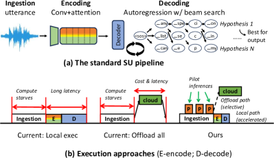
Figure 1. The SU pipeline and a comparison of execution approaches

Problem & approach

This paper sets to accelerate deep SU on resource-constrained embedded devices. It presents an on-device SU engine that integrates a local execution path and an offloading path; the local path optimized to reduce on-device latencies and the offloading selectively offloads the inputs beyond the device’s capacity, hence ensuring the overall accuracy. While the local/offloading approach is reminiscent of many ML systems, e.g. for vision and NLP (shakarami2020survey, ; yao2020deep, ; lv2022walle, ), our design specifically addresses unique challenges from speech. This is shown in Figure 1(b).

1.1. The local execution path

Challenge: temporal load imbalance

We identify a key SU inefficiency: poor resource utilization during the ingestion time. While a typical utterance spans at least several seconds, the compute is mostly idle during the ingestion period, because most of an encoder-decoder model is to be executed over a complete input, thanks to its all-to-all attention. Yet, as soon as the ingestion completes, a surge of workload — encoding and then decoding – emerges, for which long delays are directly perceived by the user.

Naively processing truncated (i.e. yet to complete) utterances during ingestion would result in significant errors, as SU models were trained on, and therefore expect, complete utterances. While some SU models are designed to process streaming inputs, they often make significant compromise on accuracy (kuo2020interspeech, ; li2020comparisone2emodel, ), as will be discussed in Section 8.

In summary, the device needs to utilize ingestion-time resources to accelerate the expensive processing that can only start after the ingestion.

Our design

Our first technique, called late contextualization, refactors an SU model so that most of encoding layers can execute in parallel to ingestion. Rather than computing all-to-all attention at each encoding layer, we make the bottom layers (closer to the input) compute only convolution, and the few top layers compute attention.

Our second techique is called pilot inference: during ingestion, SU periodically encodes and decodes the incomplete input accumulated so far. As mentioned above, inference on a truncated input will result in substantial errors, particularly near the output sequence’s end. Yet, our key insight is that the the inference’s intermediate state can assist the subsequent full inference (i.e. the one executed over the complete input). The assistance comes in multiple ways: (1) beam collapse: the full inference only needs to verify its beam search path against the path in the pilot inference, and only falls back to full beam search in case of path divergence; (2) early termination: extrapolating the output length of pilot inference, the full inference predicts the final output length and prunes astray search paths; (3) CTC leap: approximating the CTC prefix scoring (watanane2017hybridctc, ) with the scores already computed in pilot inferences.

Pilot inferences are cheap: being incremental, the $(i+1)$-th inference instance reuses of the state from the $i$-th instance, in the same way as the full inference reuses the last pilot inference instance. In this way, the total cost of pilot inference is amortized over the duration of ingestion, and scales gracefully with the input length.

Pilot inference (PI) is related to recent speculative execution for language models (kim2023speculative, ) with a key difference: while the later optimizes inference on complete inputs, PI processes successive incomplete inputs, entailing different challenges and techniques. Section 8 presents a detailed comparison.

1.2. The offloading path

Challenge: Offramps for autoregression

The common offloading paradigm works as follows. To decide whether to offload an input $x$, the device assess how likely the on-device inference yields a sufficiently accurate answer. Often, such an assessment of confidence is based on shallow processing of $x$, which is referred to as offramps in prior work. Existing offramp designs typically evaluates confidence as an ML model’s prediction entropy (NEURIPS2020_d4dd111a, ; xin-etal-2020-deebert, ). For SU however, existing offramps mismatch in two ways.

First is the confidence measure. Unlike a classification task which evaluate a model’s layers sequentially, SU’s output generation is both concurrent and iterative: it produces multiple hypotheses of probabilistic tokens; to produce each token it evaluates all the decoder layers. To complicate the issue, one hypothesis often comprises tokens that have drastically different probabilities. It was unclear how to derive one confidence score out of such a generation process.

Second is timing. Given an input, offramp represents a one-shot decision that can be taken at various times throughout the SU pipeline shown in Figure 1. While a deferred decision would have more input information for measuring the model confidence, it also incurs substantial on-device delays. The timing therefore hinges on tradeoffs between an offramp’s selectivity and overhead.

Our design

The device evaluates its offloading decision as soon as it finishes ingestion, based on the perplexity score (Jelinek1977PerplexityaMO, ) of the last pilot inference (LPI). Doing so strikes a sweet-spot: (1) as the discrepancy between the LPI and the full inference is small, their perplexity scores are also similar; (2) the device does not need to hold off the offloading decision until the slow full inference. Note that offloading before the ingestion completes does not reduce the offloading delay. As an input utterance is as small as tens of KB, the upload is typically bound by network latency; another network round trip is nevertheless needed.

1.3. Results and contributions

We implement a system called XYZ, atop two embedded platforms with 6 and 8 Arm64 cores respectively. We test XYZ on SLURP (slurp_dataset, ), a challenging speech benchmark comprising 102 hours of speech. On both ASR and SLU tasks, XYZ delivers strong accuracies with end-to-end latencies as low as 100s of ms. XYZ’s on-device execution incurs 2x lower latency as compared to popular, efficiency-optimized models running on device. Augmented with offloading, XYZ’s hybrid execution offers much higher accuracy than the on-device models at similar or lower latency; the hybrid execution offers close-to-gold accuracy (only 1% lower than SOTA), while requiring 47% – 53% less offloading than offloading all the inputs.

Towards deep SU on embedded devices, we contribute:

• An encoder-decoder architecture (convolution on bottom layers; attention on top layers), which enable late contextualization and let most of the encoding computation finished during the ingestion

• Pilot inference, a new techinque to exploit under-utilized resources during ingestion.

• An offramp design that assesses model confidence in generative, autoregressive output. This is the first mechanism for offloading generative tasks, to the best of our knowledge.

We will make our model and code publicly available.

2. Motivations

2.1. Deep SU at the edge

An unsolved task

For general SU, current models can attain low word error rate (WER) on simple utterances: e.g. WER of only 4% on LibriSpeech (Panayotov2015librispeech, ). On real-life speech as in the SLURP dataset (slurp_dataset, ), however, WER can be as high as 20% (Hannun2021TheHO, ). Deep models reduce WER significantly, albeit requiring higher resources beyond an embedded device.

Our system model

The devices have several CPU cores (no more than 8) and around 100 MB of memory budget (lebeck2020memoryos, ; soyoon2021androidmemory, ). The devices are wirelessly connected to the cloud services; yet, cloud invocations incur monetary cost. For SU tasks, users expect low latency after they finish speaking to the devices. The device detects the beginning and end of an utterance with well-known, lightweight algorithms (Liu2015AccurateEW, ; martin2001speechdetection, ).

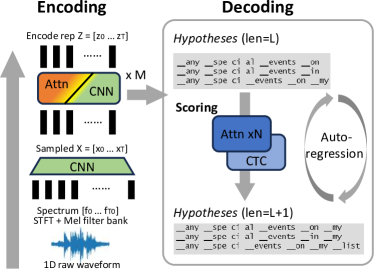
Figure 2. The vanilla speech understanding pipeline. The input of SU tasks, an 1D raw wavform of the audio, will first go through STFT+Mel filter bank to get spectrum, then processed by encoder to get intermediate encode representation, and finally decoded in an autoregressive fashion by hybrid transformer/CTC decoder coupled with beam search method

2.2. A primer on SU pipelines

A typical pipeline as in Figure 2 builds atop attention-based models, as well as autoregressive beam search (conformer-2020, ; peng2022branchformer, ; baevski2020wav2vec, ).

Module 1: The encoding process

Typically, the encoder in an SU model consists of multiple layers that combine convolution and attention-based elements. This design can be found in models such as Conformer (conformer-2020, ), Branchformer (peng2022branchformer, ), Wav2vec (baevski2020wav2vec, ), and HuBERT (hsu2021hubert, ). During operation, as shown in Figure 2 left part, the 1-D speech data will be broke in to frames and undergoes STFT and Mel-filter bank methods to create a 2D spectrum that have $f_{1}...f_{T_{o}}$, each $f_{i}$ is the processed frequency component of that time frame. The 2D spectrum $[f_{1},...,f_{T_{o}}]$ is then processed by a few convolutional layers for downsampling, $X=x_{1},...,x_{T}$ is get from $X=subsampling([f_{1},...,f_{T_{o}}])$. The X is subsequently passes through multiple encoder layers that include both convolutional and transformer component and get the latent speech representation $Z$ among the same time frames $z_{1},...,z_{T}$ like X, $Z=encoders(X)$. This entire encoding process is a one-pass operation, providing an intermediate representation of the speech signal framewise with a specific dimension.

Module 2: The decoding process

The decoder typically includes a transformer decoder and a CTC decoder. The rationale is that the transformer decoder comprises several transformer layers excel in maintaining language consistency, while the CTC decoder is a linear layer primarily focused on audio features.

The generation of the final transcript involves an autoregressive beam search process as shown in Figure 2 right part, with tokens generated one by one. The beam search employs a specific beam width (k), maintaining k developing hypotheses during the decoding process. In decoding, the CTC decoder first calculates posterior token probabilities $p(z_{i}=c|Z)$ for each frame $z_{i}$ of the encoder output. Beginning with the ”¡sos¿” (start of the sentence) token, the transformer decoder calculates the next token $c$’s posterior probabilities based on current partial hypothesis $g$ and speech latent representation and get $p_{attn}(c|g,Z)$, combine with the previous token probability we have $p_{attn}((g,c)|Z)$. The CTC prefix scorer, utilizing dynamic programming methods, further calculates CTC prefix probabilities $p_{ctc}((g,c,...)|Z)$ based on newly developed hypotheses $(g,c)$ and the CTC framewise output$p(z_{i}=c|Z)$. The best K hypotheses with highest $\lambda logp_{attn}((g,c)|Z)+(1-\lambda)logp_{ctc}((g,c,...)|Z)$ are retained in the beam for the subsequent rounds of decoding, based on a weighted sum of probabilities from the transformer decoder and CTC prefix scorer. The decoding process concludes when the completed hypothesis significantly outperforms the developing hypotheses, as described in (watanane2017hybridctc, ).

2.3. Observations & challenges

Observation 1: steady, streaming ingestion.

A typical spoken input lasts as long as 3–5 seconds  (slurp_dataset, ; Panayotov2015librispeech, ). In contrast to common vision and NLP systems which usually expect a complete input unit (e.g. a image or a sentence) upon model invocations, an SU system receives its input by pieces.

Observation 2: input context matters to accuracy.

The information in the input audio is distributed throughout its entire duration, with the entirety of the audio serving as the context for each individual part. While waiting for data ingestion may seem to hinder resource efficiency, it is a necessity for attention models. The all-to-all attention mechanism in transformer-based models is the key to their superiority in NLP and speech-related tasks. This mechanism leverages contextual information from the complete dataset to generate results with better language consistency. As shown in prior work (Jan2015NIPS, ; peng2022branchformer, ; conformer-2020, ), any portion of the output should take into account the whole input (i.e. the context). As an anecdote, in time-related phrases, words like “calendar” or “reminder” should be assigned with higher probabilities. Partial input data with incomplete context can significantly impair the model’s decoding accuracy. As such, a common practice is for the models to wait for ingestion completion (pundak2018deepcontext, ).

Challenge 1: Underutilized resources during ingestion As previously mentioned, there is an imbalance in resource utilization throughout the operation of the SU system. The CPU remains idle during ingestion, while it becomes busy during the time-consuming encoding and decoding processes. This has motivated us to explore opportunities for offloading a portion of the encoding and decoding computations during the ingestion period.

Observation 3: decoding wraps around numerous neural function evaluations (NFEs).

Unique to SU, decoding with hybrid scorers is popular (watanane2017hybridctc, ). In each beam search round, hypotheses are scored by both the transformer and CTC prefix scorer. Prior work deem both scorers vital: the transformer contributes to language consistency; CTC exploits acoustic features. Notably, the CTC scorer can be slow, as its dynamic programming algorithm sees lower parallelism compared to transformers.

Such a hybrid decoding exhibits high complexity and also exposes accuracy/latency trade-offs. Beam size $N$ controls the search width, while beam search length $L$ controls the search depth. If we use $NFE$ to denote the number of neural function evaluations per round (needed by transformer/CTC scorers), the total decoding complexity is roughly $O(N\times M\times NFE)$, if assuming a fixed beam size throughout the process.

Interestingly, we observe that $L$ is redundant: with popular SU pipelines and benchmarks, the average $L$ is ~18, much longer than the true outputs ( ~11 on average).

Challenge 2: Long decoding latency.

For the above reasons, the decoding is slow on typical edge devices. As we will show in section 7, an Armv8 CPU takes around 1 second to process a typical utterance, far exceeding user’s perception threshold at a few hundred milliseconds. Unfortunately, mobile GPUs would not help much. Our experiments on Nvidia’s Ampere mobile GPUs are even 1.6x slower than CPUs on the same board (see Table 1, 6CB). This is likely due to the irregular decoding workloads, especially the CTC scorer, leaving the GPU hardware parallelism underutilized.

3. XYZ Overview

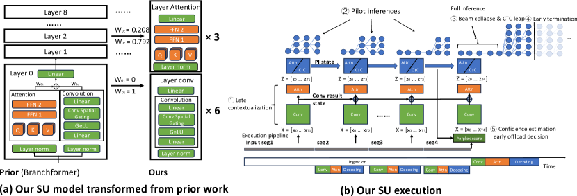
Figure 3. Overview. (a) Compared to a popular model (left), our model (right) shifts much of the encoding computation to bottom layers, allowing them to be executed in a streaming fashion during ingestion. (b) Execution pipeline of XYZ. Our system performs pilot inference periodically on partial input, and use the pilot inference result to speedup the final inference

3.1. The on-device model

Encoder: late contextualization

XYZ features a novel encoder designed shown in Figure 3(a). and (b).( ) which separate the streaming convolutional part and non-streaming transformer part to enable more than half of the computation to get done during data ingestion.

As shown in Figure 3(a)., our model is motivated by the Branchformer (peng2022branchformer, ), which have parallel convolutional and transformer blocks in each layer for local and contextual feature extraction. The learned weight shows the redundancy in the model. Our model keeps the blocks that have higher weight and rearrange them to make the convolutional layers which enable streaming processing at the beginning to hide the computation latency into the ingestion time.

Decoder

As shown in  Figure 3, XYZ has two versions of the decoder for pilot inference ( ) and full inference. By default, the pilot decoder shares the same structure and weights with the full decoder but has a smaller beam size.

The training details can be found in Section 6.

3.2. The operations

As shown in Figure 3(b)., XYZ ingests segments of voice input $x_{1..n}$. On each segment, XYZ executes the cgMLP (convolutional) encoder layers per-segment results $y_{i}$ that can be combined later ( ). Periodically, the device executes pilot inference ( ) with idle compute resources: sending the accumulated segments $\{z^{\prime}_{i=1..T_{k}}\}$ to the attentive encoding layers to get $\{z_{i=1..T_{k}}\}$, followed by the decoding process that generates a sequence of tentative tokens, which we refer to as a “pilot output”. Over the course of ingesting an input, XYZ may execute pilot inference multiple times, each time on an increasingly longer input. The execution of pilot inferences is incremental: each inference reuses computation of the previous instances. The frequency of pilot inferences is a configuration parameter to be evaluated experimentally. Essentially, this periodical pilot inference tries to extract as much information as possible from the partial inputs, during the ingestion. This information benefits the subsequent execution in two ways. For local execution, the information aids in speeding up decoding. For hybrid execution, the information contributes to local confidence estimation and the selection of the execution path.

Once the ingestion is over (detected with auxiliary means as in prior work. e.g pause (Liu2015AccurateEW, )), the device evaluates the offloading decision immediately (and aborts the ongoing pilot inference, if any) by computing the confidence score of the most recent pilot output( ). By doing so, the decision can be made without waiting for inference on the complete input $\{x_{i=1..T}\}$; since this pilot inference is based on an input with length closest to the complete input, its confidence is close to the full length decoding confidence.

If confidence is low, XYZ offloads the input as waveform and waits for results; otherwise, it finishes encoding $\{x_{i=1..T}\}$ and executes the full decoding over $\{z_{i=1..T}\}$. Although the device cannot directly emit the pilot output because of the latter’s high errors, the decoding benefits from pilot output in crucial ways: to reduce the beam search width( ), to approximate the CTC prefix scores( ), and to help with the beam search early termination( ).

3.3. Applicability

Our key techniques can be applied independently or in combination to existing SU deployment. (1) Late contextualization and pilot inference both speed up local execution; they can be applied separately to existing models. Specifically, pilot inference can be applied to existing unmodified models, such as branchformer, HuBERT, etc. Notably, it is compatible with both CTC decoding (classic), attention decoding (modern, such as in Whisper (pmlr-v202-radford23a, )), or a hybrid one, as we will show in Section 7. (2) Offramps optimizes offloading decisions; it can be applied to existing local models (without our enhancement) in order to form a hybrid solution. The caveat is that the decision has to be evaluated on full decoding sequence, which incurs extra delays as compared to our system. Our techniques require light modifications to the existing SU implementations. It does not requires to develop new ML operators. Late contextualization requires to train a new model architecture; the model can run atop existing ML libraries and toolkits such as ONNX runtime and ESPnet. Pilot inference and offramps modify the SU pipeline logic, which is implemented in Python code on CPU.

4. The local execution path

This section focuses on pilot inference for local execution.

4.1. The mechanisms

Pilot inference works periodically on partial data as shown in  Figure 3(b). ( ). XYZ refrains from performing pilot inference on excessively short data as it is hard to generate meaningful result with too short partial data. During data ingestion starting from $T_{0}$s, the system conducts pilot inference on partial data periodically with a pre-defined granularity of $\delta t$s, intended to complete within $\delta t$s. In each round of pilot inference, the system utilizes the same encoder and the pilot decoder to engage in beam search inference with a beam size of k. Supposing the pilot inference is performed on data length $T_{0}+n\delta t$s, it will take at most $\delta t$s to finish and the results cover the full data that have length range between $[T_{0}+(n+1)\delta t$s, $T_{0}+(n+2)\delta t$s]. To manage the runtime of pilot inference, a token limit of $l$ tokens is set. Following the decoding of $l$ tokens, the hypothesis with the highest probability is chosen as the reference hypothesis for local execution or hybrid execution path decisions. The reference hypothesis, denoted as $yp_{1:n}=(yp_{1},\ldots,yp_{n})$, offers the potential to accelerate the full inference process from multiple perspectives mentioned in the next few subsection.

Hyperparamters

Several key parameters in pilot inference require pre-operation definition. These parameters include granularity $\delta t$, beam size $k$, and the maximum token length for beam search inference, denoted as $l$. These hyperparameters are determined through heuristic methods based on experimental experience. The granularity needs to be established initially. Typically, the system anticipates that the longest partial data covers at least  70% of the full-length data. To achieve this, the granularity is expected to satisfy $\delta t<0.2T$. It’s important to note that the granularity doesn’t have to remain a fixed number throughout system operation. As data lengthens, the pilot inference take longer time as shown in Figure 3(b). ( ) comparing the different pilot inference, the granularity can also expand. The beam size for pilot inference is set at 60% of the beam size used for full decoding to ensure lightweight pilot inference while maintaining fidelity. The inference length is determined based on average inference length. If the average inference length is $l_{full}$, XYZ sets $l$ to be $0.7*l_{full}$.

Incremental execution

The pilot inference based full decoding acceleration techniques (which will be elaborated in the following sub-sections) can also be adopted in the pilot inference execution. More specifically, the reference based beam collapse can be adopted in the pilot inference. In our system, as shown in Figure 3(b). ( ), from the second pilot inference, each pilot inference can take reference hypothesis from the previous pilot inference and perform beam size reduction in the pilot beam search procedure. Incremental execution is critical for pilot inference runtime reduction.

4.2. Optimization 1: beam collapse

Assumption Most tokens of the full transcript should be the best token in the beam search decoding process at the corresponding round. For the beginning part of the transcript, the reference transcript from pilot inference should share most of the tokens the same with the final transcript. What we do Base on this assumption, during full inference, starting from the first token, in each inference round before predicting the next token probability using the scorers, the system attempts to validate the reference hypothesis. It checks the latest token in the current best hypothesis, $y_{i}$. If $y_{i}=yp_{i}$, the token is validated, and the system retains only the best hypothesis for the subsequent token calculation in this round. Complexity reduction This verification reduces the number of running hypothesis for predicting the next token to 1, also reduces required NFE to 1 / beam size. Why such approximation is acceptable The approximation is reasonable because of two point: the reference result is from pilot inference works on most part of the data by design. The verification step also partially secures the inference not to be deviated by the potential wrong part in the reference transcript.

4.3. Optimization 2: early termination of beam search

Assumption The reference inference results can reflect the final transcript length, as the token number grows proportionally as time grows. What we do The system predicts the final inference length using three key parameters: the length of the partial data, $l_{partial}$ obtained in the latest pilot inference; the full data length, $l_{full}$; and the token count of the reference hypothesis, $n_{p}$. The calculation for the full inference length is expressed as $n=l_{full}/l_{partial}*n_{p}+C$. $C$ represents a tunable constant that loose the early termination in full inference. During the full inference, when the full inference reaches the predicted length n, if there are terminated hypotheses, the system terminates the beam search inference. Otherwise, the system continues inference until at least one hypothesis ends before terminating the process. Complexity reduction Assume the vanilla beam search length is $l_{v}$, the early termination can save $(l_{v}-n)$ round of NFE calculation. Why such approximation is acceptable The approximation works well because the tokens distribute evenly among time statistically. The loose factor C can also help to decrease the deletion error that introduced by too aggressive early termination.

Algorithm 1 Algorithm modified with CTC leap for CTC prefix scoring speedup. The highlighted part is our modification to reuse the calculation in pilot inference and skip part of the calculation. The remaining parts are the same as the hybrid CTC/attention algorithm (watanane2017hybridctc, ).

4.4. Optimization 3: fast prefix scoring with CTC leap

Assumption Some of the CTC prefix scoring computation during pilot inference can be reused in the full inference process. The original CTC prefix scoring requires recursively calculated among all the time frame $[1,T]$. In pilot inference, calculation among $[1,T_{pilot}]$ has been done. The system just need to finish the calculation among $[T_{pilot},T]$ What we do We propose CTC leap to help accelerate the CTC prefix scoring step in Hybrid CTC/Attention decoding (HD) algorithm (watanane2017hybridctc, ) by reusing the computation in pilot inference. The algorithm modified with CTC leap is shown in  algorithm 1 The CTC prefix scoring in HD algorithm is a modified version of forward algorithm that help calculate the prefix CTC probabilities among all the time frames. In the algorithm, the prefix forward probability of prefix h among 1 to t time frames is denoted as $r_{t}^{(n)}(h)$ and $r_{t}^{(b)}(h)$, for the prefix end with non-blank and blank token. In the algorithm, the prefix h will be divided into the last token c, which is the new token that to be developed, and the prefix part g. basically (g, c) equals h. If c is the ¡eos¿ token, same with original algorithm, $r_{T}^{(n)}(g)+r_{T}^{(b)}(g)$ by definition is the final overall probability result . When c is other tokens, the $r_{[1...T]}^{(n)}(h)$ and $r_{[1...T]}^{(b)}(h)$ is calculated through the loop between line 11-14 recursively. The $\psi$ is the final cumulative prefix probability among all the time frame, calculated based on the $r_{[1...T]}^{(n)}(g)$ and $r_{[1...T]}^{(b)}(g)$ and the CTC posterior probability $p(z_{t}=c|X)$. In the calculation, the bottleneck is the recursive loop calculation of $r_{[1...T]}^{(n)}(h)$ and $r_{[1...T]}^{(b)}(h)$. Different from the original algorithm, as high lighted in algorithm 1, in our algorithm, we reuse the $r_{[1...Tpilot*r_{factor}]}^{(n)}(h)$ and $r_{[1...Tpilot*r_{factor}]}^{(b)}(h)$ from pilot inference to skip the calculation from time frame 1 to $Tpilot*r_{factor}$ and only do $Tpilot*r_{factor}$ to $T$ when beam collapse happens. This could work because if the beam collapse happens, the reference hypothesis from pilot inference should also include prefix g, as well as the calculation result of $r_{[1...Tpilot*r_{factor}]}^{(n)}(h)$ and $r_{[1...Tpilot*r_{factor}]}^{(b)}(h)$. Complexity reduction When the speedup requirement is met (pilot inference token is verified), the CTC prefix probability calculation in this round can be saved by $r_{factor}*T_{pilot}/T*NFE_{CTC}$. Why such approximation is acceptable We reused the $r_{[1...Tpilot*r_{factor}]}^{(n)}(h)$ and $r_{[1...Tpilot*r_{factor}]}^{(b)}(h)$ in the pilot inference. We argue that the reused computation result is a good approximation. It is because essentially the reused calculation are (1) ultimately calculated from CTC posterior $p(z_{t}=c|X)$, which is calculated framewisely with CTC linear layer, thus the beginning part does not depend on the latter part. (2) the reused calculation is also based on a forward recursive algorithm, make it independent to the latter time frame.

4.5. Implications of approximation

Approximate execution is common to SU and more general autoregressive system like LLM, because the whole thing is statistically in nature; and people often make approximate at their discretion, as long as the approximation can be empirically validated. The speculative decoding technique in (kim2023speculative, ) also involves tentative hypothesis validation. The beam search end estimation technique in (kasai2022beam, ) introduce tunable parameter ”patience factor” to help tune the beam search length. The truncate CTC prefix scoring in (miao2020onlinehybrid, ) estimate the CTC prefix alignment with time frame to save part of the computation. Different from these method, our system can better work on these estimation with the help of reference result from pilot inference.

5. The offloading path

While the above designs accelerate the local execution, the SU task accuracy is nevertheless bound by the model size on the device. To deliver SOTA accuracy, we further augment the SU pipeline with cloud execution. The key challenges are twofold. (1) The device should estimate confidence (as the offloading criteria). Existing method (xin-etal-2020-deebert, ) used in classification tasks cannot be directly applied to the generative SU task. It is because it works with the BERT style encoder, only take first frame of the output for classification and cannot take the full input into consideration. (2) The device should do so without delaying the local processing. It cannot, for example, simply evaluate the decision after full inference, as this would result in extended local decoding times for all inputs. It also cannot offload prior to ingestion completion: as each voice input is typically tens of KB to $\sim$300 KB for speech less than 10 s, the offloading is bound by network round trips (RTTs); the device would still need one RTT to offload the whole input, after the ingestion completes.

Confidence estimation

Perplexing Score-Based Approach The perplexing score is derived from the reciprocal of the average probability of all tokens in the hypothesis, calculated by $exp(-\frac{1}{l}\sum_{i=0}^{l}log(p(y_{i}|y_{<i})))$. A high perplexing score indicates low confidence of the local model with the data. The system sets different thresholds for the perplexing score and offloads data that surpasses these thresholds.

RNN-Based Approach During beam search, the system gathers the probability of each token in the hypothesis. This fine-grained probability information better represents the local confidence in the data. Different patterns in the token probability sequence may signify different meanings. For instance, sequences of low-probability tokens often imply a lack of model confidence in the semantic correctness of an entire output span. Conversely, if such tokens are scattered, it could be attributed to acoustic noise while the output remains mostly correct. Defining rules manually can be challenging, so we adopt a learning-based approach: constructing a lightweight BiLSTM model to predict the local SU confidence. To achieve this, we label the dev set data into two classes based on their accuracy and the threshold, and then train the BiLSTM model to predict the classes. The model’s output serves a similar role as the perplexing score.

CNN-Based Approach The intermediate results from the encoder contain rich information about the data but possess significantly higher dimensions compared to the token probability sequence. To address this, we propose a CNN-based approach to assist in down sampling the intermediate results and predict the confidence. Similar to the RNN-based approach, we train the CNN model on the develop set to predict the local SU accuracy. It’s noteworthy that during the design of the CNN network, we observed that the CNN model typically require a larger model size compared to the RNN approach. This issue makes it less practical.

Decision timing

The XYZ makes the offloading decision precisely when the data ingestion is completed, along with the pilot inference result. This is shown in Figure 3(b).( ) Both the perplexing score method and the BiLSTM method require post-decoding results. However, if the system performs confidence estimation after the full local execution, the offloaded data will also suffer from local decoding latency. To circumvent this, the system executes the aforementioned methods on the latest pilot inference result, , i.e. the 3rd pilot inference in Figure 3(b).( ) enabling the system to make the execution path decision simultaneously with the completion of data ingestion. This approach is founded on the assumption that the partial data in the pilot inference can reflect corresponding information in the full-length data.

6. Implementation

We implemented XYZ using 4K SLOC in Python, built upon the renowned speech toolkit ESPnet.

Model training details

To train our model, we first configure and train an example branchformer model base on the memory and latency budget. In the experiment case, 9 layers of encoder and 1 layer of decoder. To construct XYZ’s model, assume there are k transformer blocks with weights exceeding a threshold h in the trained branchformer encoder, we design the encoder with N-k-1 CNN layers followed by transformer k+1 layers. In the experiment, we get 2+1 transformer and 9-2-1 CNN layers. This design is then trained from scratch on the same dataset, with the same decoder design branchformer model has. The comparison with the branchformer encoder is illustrated in  Figure 3(a).

Operation details

During system operation on the SLURP dataset, we set the shortest partial data for pilot inference at 1.5 seconds. This granularity is determined based on hardware specifications, tested across 0.5s - 2s. The pilot beam size is set to be 3, which is 60% of the full inference beam size of 5. The length limit for pilot inference tokens is set to be 15. The length prediction $C$ is set to be 5.

Hybrid execution details

For hybrid execution and offloading decision-making, in the perplexing score-based method, we calculate the perplexing score based on the reference result from the pilot inference. Regarding the LSTM and CNN-based methods, we utilize the full dev set in SLURP as the training set for the LSTM and CNN models. The CNN approach employs a CNN model that takes the encoder’s full output as input. The CNN model has two convolutional layers and two fully connected layers, with 192.5 M parameters. The LSTM approach employs a BiLSTM model that takes CTC prefix probability and transformer token-wise probability of the reference result as the input. The LSTM model we adopted is a 1-layer BiLSTM model with 11.1k parameters. The training task is defined as a binary classification task, where a local execution WER ¿ 0.1 is labeled as 1, and otherwise as 0. During operation, the BiLSTM and CNN process the respective input and provide predictions, representing the probability of the data having a WER ¿ 0.1 as a float number between 0 and 1. Further, we set thresholds on this output for different offloading accuracy targets.

7. Evaluation

We answer the following questions:

• Can XYZ reduce latency with competitive accuracy?

• XYZ’s local path: what is its efficacy?

• XYZ’s offloading path: what is its efficacy?

7.1. Methodology

Test platforms

As shown in Table 1, we test on two embedded boards: 6CB with an efficiency-oriented SoC with six cores, whereas 8CB with a performance-oriented SoC with eight cores. Our experiments focus on CPUs, though our idea applies to GPUs as well.

We run the cloud runtime on platform with an x86/NVidia machine and measure accuracy. To better estimate the cloud offloading delay, we measure Microsoft’s speech service (microsoft_azure_speech, ): we invoke the Azure APIs to offload waveforms and record each waveform’s end-to-end wall time. Our measurement runs from the US east coast and invokes datacenters on the east coast. For each input, we repeat the test on enterprise WiFi (bandwidth in 100s of MB and RTT in ms) and on 5G networks, and take the average. Note that we do not use Azure speech for accuracy evaluation, as we find its accuracy inferior to the SOTA model (2 pass SLU (arora2022two, )) used by us.

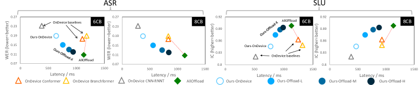
Figure 4. Our system deliver low delays and competitive accuracy. Compared to other local models marked with $\bigtriangleup$$\bigtriangleup$$\bigtriangleup$, our local execution Ours-OnDevice $\bigcirc$ show similar accuracies at much lower delays or higher accuracies; Compared to AllOffload

 

, our hybrid executions $\bullet$ $\bullet$ $\bullet$ show much lower delays with little accuracy loss.

Table 1. Embedded platforms used in evaluation

Table 2. Overview of SLURP dataset for SU tasks

Dataset and model training

We run our experiments on SLURP (slurp_dataset, ) as summarized in Table 2. Comprising 102 hours of speech, SLURP’s utterances are complex and closer to daily human speech (e.g. “within the past three months how many meetings did i have with mr richards”), as opposed to short commands (e.g. “light on”) in many other datasets. Of all 141,530 utterances, we use 119,880 (85%) for training and the rest for dev set and test set. The accuracy and latency are reported from the test set data range from 2s to 6s.

Metrics

We follow the common practice. Accuracy. For ASR, we report word error rate (WER): the discrepancy between the model output and the ground truth transcript, defined as count of errors (substitutions, deletions, insertions) normalized by the sentence length. For SLU, we report the intent classification accuracy (IC).

Latency. (1) We report user-perceive latency (yu2016automatic, ): the elapsed time from a user completing her utterance to the system emitting the complete SU result. (2) We further report the real time factor (RTF): the user-perceived latency normalized by the input utterance’s duration.

Baselines

We compare the following designs.

• OnDevice: SU completely runs on device, for which we test a wide selection of model architectures: Conformer (conformer-2020, ), Branchformer (peng2022branchformer, ), and CNN-RNNT (zhang2020transformer, ). Note that CNN-RNNT is streaming, with 640ms chunks as in prior work. For fair comparison, we choose models sizes to be around 30M parameters, which are comparable to ours. They are summarized in Table 3.

• AllOffload: The device offloads all inputs, for which the cloud runs a SOTA model (arora2022two, ): a two-pass end-to-end SLU model with one conformer-based encoder, one conformer-based deliberation encoder, two transformer-based decoders for the two passes, and a pretrained BERT language model. It has ¿10x parameters as compared to the local models above. We refer to its accuracy as gold.

• NaiveHybrid: To combine OnDevice and AllOffload, execute any input with probability $\alpha$ for local execution and $(1-\alpha)$ for offloading.

• Ours: By varying the confidence threshold $\theta$, we tested a range of variants which we refer to as Ours-OnDevice (0% offloaded), Ours-Offload-L (25%), Ours-Offload-M (47%), and Ours-Offload-H (63%).

7.2. End-to-end results

As demonstrated in Figure 4, XYZ is able to deliver a wide range of accuracies (from modest to nearly gold), with latencies as low as 100s of ms.

Compared to OnDevice, all variants of our system are better in the latency - accuracy trade-off. Ours-Offload-M and Ours-Offload-H achieve much higher accuracy (WER lower by 5%; IC higher by 2.5%) at similar or lower latencies; Ours-OnDevice achieves similar accuracies while reducing latencies by around 2x.

Compared to AllOffload, Ours-Offload-L and Ours-Offload-M reduce the overall latency by as much as 37% and 27% while seeing minor degradation in accuracy (no more than 4% WER and 2% of IC). They process 75% and 53% of inputs on device, reducing the need for cloud invocations by 2x or more. Ours-Offload-H has negligible accuracy degradation (¡0.5% of IC) while still reducing latency by 20% and offload needs by 37%.

NaiveHybrid, shown as the dash lines interpolating between OnDevice and AllOffload on Figure 4, always shows inferior accuracy or latency to ours.

7.3. Efficacy of our local path

As shown in Figure 4, our local-only execution (Ours-OnDevice) significantly outperforms OnDevice, reducing latencies by 1.7x - 2.2x at similar accuracies. We next break down the benefit into two parts: encoding and decoding.

Table 3. Our local encoder executes mostly streaming FLOPs, for which latency can be hidden behind IO; doing so does not compromise the final accuracy. FLOPs numbers normalized to 1 second of input. Our local execution path incur lower latencies (reported as RTF) for both encoding and decoding, as compared to other on-device models.

Encoding speedup

We strike a sweet spot between speed (by processing inputs in a streaming fashion) and accuracy (by attending to the whole input). Table 3 breaks down the encoding computation. Compared to encoders with all attention layers (Con/Branchformers) where 67% and 38% FLOPs are non-streaming (i.e. must execute after ingestion), 92% FLOPs of ours is streaming, for which the latency is hidden behind the ingestion. Meanwhile, we do not lose much accuracy compared to Con/Branchformers, as our design runs three attention layers after ingestion ends. This design reduces the latency by 3.6x - 5.4x (220 – 345 ms or 0.07 – 0.11 RTF) as shown in Table 3. Compared to full streaming encoders (CNN+RNNT) for which 100% FLOPs is streaming, our accuracy is much higher by 4% in WER and 2.6% in IC, because the former critically lacks attention over the whole input. Meanwhile, our encoding latency is only higher by 0.005 RTF (15 ms for a 3 second input) as in Table 3. Such a difference is dwarfed by the difference in decoding delays.

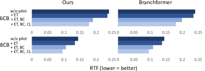
Figure 5. An ablation study of pilot inference, showing that all its three optimizations contribute to lower latency significantly. It also shows that pilot inference can apply to on-device models (e.g. Branchformer) other than ours. ET: Early termination, BC: Beam collapse, CL: CTC Leap

Decoding speedup

Our design shows 1.5x lower decoding delays compares to OnDevice (Table 3). All three techniques show contribution to the overall speedup as Figure 5 shows. We also demonstrate the decoding speedup method on branchformer. The speedup ratio is similar with it on ours model, shows that our speedup method is applicable on general transformer based encoder-decoder speech model.

The incremental nature of pilot inference is crucial, as it amortizes the decoding cost over the past input, making the cost scale slower as the input grows. Turning off the incremental design (i.e. each pilot inference starts from the input’s start) increases the average decoding delay by 30%, from 156 ms to 205 ms; it increases the 90th percentile delay by 40%, from 198 ms to 282 ms. Reduction in pilot inference cost allows the system to execute pilot inference more frequently.

Table 4. Pilot inference significantly reduces the end-to-end delay. It benefits our local-only execution (Ours-NoOffload) as well as our hybrid executions (Ours-Offload-X), for which the offloading are made more selective.

We further study the impact of pilot inference’s eagerness: during ingestion, every $\tau$ seconds XYZ decodes the input it has accumulated so far. Lower $\tau$ reduces the discrepancy between the last pilot inference and the full decoding, therefore improving the full decoding speed and quality. As shown in Table 4, 4x reduction in $\tau$ (from 2s to 0.5 s) reduces final RTF by 0.025. further reduction in $\tau$ helps the pilot inference get longer partial data that cover more part of the full length data In exchange, the expense is that the ingestion consumes more compute. $\tau$ is lower bounded by the available compute resource during ingestion. For instance, 8CB can sustain $\tau=0.5s$ while 6CB cannot.

Table 5. Our offloading strategies based on sequence modeling outperform NaiveHybrid (random selection) and DeeBERT (sequence classification, failing to produce useful results). In the experiment, we tune $\theta$ and $\alpha$ to meet WER goals and compare delays and offloading ratio

7.4. Efficacy of our offloading path

XYZ effectively identifies and uploads the inputs that would suffer from low accuracy on device.

Comparison vs. NaiveHybrid

We replace XYZ’s offloading strategy with NaiveHybrid while keeping all other optimizations. The results in Table 5 show that to reach the same accuracy (WER), NaiveHybrid has to offload up to 2x more inputs. The extra offloading translates to higher cloud cost as well as higher latency (0.06 RTF; 180 ms on average).

Figure 6 shows detailed offloading decisions: For Ours-Offload-M (WER=0.13) and Ours-Offload-H (WER=0.12), XYZ offloads the majority of target inputs, while still executing the majority of non-target inputs on device. This is much higher than NaiveHybrid which make decisions “by chance”.

Comparison vs. DeeBERT

Our experiment also shows that a popular early-exit approach (xin-etal-2020-deebert, ), estimating model confidence with linear classifiers inserted after the encoder, performs poorly for encoder-decoder SU models. We implemented such an approach: training linear classifiers atop the first output frame embedding from the encoder. We could not get meaningful results – the classifier is no better than a random predictor. This highlights the challenge of predicting SU confidence, for which the entire generated sequence (not just the 1st frame from encoding) must be considered.

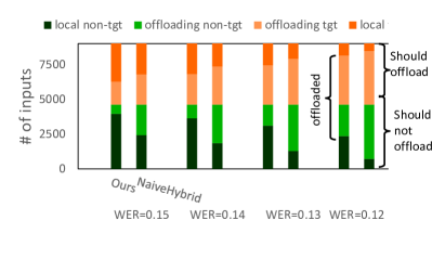
Figure 6. Our design shows good selectivity in making offloading decisions, offloading much fewer inputs compared to NaiveHybrid achieving similar accuracies.

Choice of sequence modeling strategies

The sequence modeling techniques in Section 6 (CNN, LSTM, and perplexity) can well estimate the model confidence. Table 5 shows that LSTM offers the lowest offloading percentage and RTF. PPL perform slightly worse, but as perplexity has much lower computational complexity (no training, no parameters), we deem PPL as the most suitable.

How PI affects offloading decisions?

Recall that XYZ makes offloading decisions based on the last pilot inference (section 5). We answer the following questions. (1) How does pilot inference’s execution plan affect offloading decisions? Our results show that finer granularity (i.e. smaller discrepancy between the pilot and the full inference) leads to better estimation of model confidence, which results in more accurate offloading decisions. For instance in Table 4, to maintain the accuracy at WER=0.15, reducing $\tau$ from 2 s to 0.5 s reduces the offloaded inputs by 14%, which translates to 93 ms lower end-to-end delay. (2) What if we make offloading decisions based on the full decoding outcome? Our results show that while the offloading selectivity slightly improves, the end-to-end latency is much higher (by 264 ms or 0.088 RTF), because the device makes offloading decisions much late – after ingesting the whole input and executing full decoding.

7.5. Sensitivity to system parameters

Device hardware and network delays

With different device hardware, our local execution maintains consistent speed advantages over baselines, as shown by the comparison 6CB and 8CB, Figure 4. Besides, faster device computation can perform pilot inference with smaller granularity. Our measurement was from decent network conditions that favor offloaded executions. With longer network delays, XYZ’s benefit would be even more pronounced, as fast local executions and selective offloading will be more important. If network delays further reduce, the latency gap between our system and OffloadAll may narrow. Even if that happens, our benefit of reduced cloud cost will still remain.

Computation and Energy Efficiency

In terms of energy costs on mobile devices, our system generally delivers energy savings. Mobile devices often exhibit high background energy consumption when not in sleep mode. During ingestion, the pilot inference may only result in a roughly 2x increase in energy costs. Nevertheless, the savings during full decoding are substantial with our system. Offloading reduce the local decoding cost to 0. Local execution with XYZ can reduce the RTF by 50%, leading to significant energy savings and enabling mobile devices to return to sleep mode earlier.

8. Related work

LLM speculative decoding (SD)

Speculative decoding for LLM decoding speedup includes a fast generating and verify later pattern. Some examples are: copy and verify from input  (yang2023inference, ), use non-autoregressive translation methods  (xia2022lossless, ), shallow decoder and parallel decoding (sun2021instantaneous, ), different decoder for token with different confidence (kim2023speculative, ). Comparing SD to our pilot inference Tasks: Pilot inference targets streaming SU task, which has the temporal workload imbalance problem. SD targets LLM decoding, faces the underutilized hardware parallelism issue. Solutions: Pilot inference work with incomplete streaming input. SD deals with a complete input, spawning fast and slow tasks concurrently. SD’s speedup is contingent upon high hardware parallelism, which is lacking on an embedded device. The connection in between is that the full decoding benefit from an earlier decoding process.

Streaming speech procssing

Streaming approaches like transducer-based models (graves2012sequence, ; rao2017exploring, ; zhang2020transformer, ) process the data in a chunk-wise fashion, initiating transcription during data ingestion and reduces the latency. However, they only possess partial data during streaming processing and lack contextual information. Compare to attention-based model (baevski2020wav2vec, ; conformer-2020, ; peng2022branchformer, ), the accuracy of streaming models is inferior  (li2020comparisone2emodel, ). Our work focuses on speedup attention-based models.

Offloading and hybrid execution

Device-cloud collaboration (mach2017mobileedgecomputing, ) is well-discussed in general scenarios. The cost during collaboration is an important concern (qualcomm2023hybridcost, ; qualcomm2023futurehybridai, ; microsoft2023azurehybridbenefit, ). A concurrent work optimizes SU for microcontrollers in the local/cloud setting (anonymous2023speechhybrid, ). Yet, incapable of deep SU models (with only a few MBs of memory), microcontrollers only run an inference cache, rather than a complete engine like XYZ. These two projects have orthogonal contributions; they do not depend each other.

Comparing CTC Leap with the Online CTC/Attention Method

Online CTC/attention method  (miao2020onlinehybrid, ) reduces CTC scoring latency by Truncated CTC method. Both Truncated CTC and CTC leap try to skip part of the CTC prefix scoring computation among all the time frame. The difference is that: we reuse the CTC computation from the pilot inference to skip the beginning part; whereas they stop early by using the CTC peak heuristics to skip the latter part. Notably, same with the original approach  (watanane2017hybridctc, ) our method still includes all the time frames while they choose to drop some temporal information, which may include crucial information for CTC.

9. Conclusions

We present XYZ, a novel system for fast speech processing in SU tasks. XYZ contributes late contextualization, beam collapse/ termination, and CTC leap for local execution; and confidence estimation for selective offloading. All optimizations combined, XYZ speeds up its local path by 2x and reduces the offloading needs by 2x in its offloading path.

References

- [1] Anonymous. Leveraging cache to enable slu on tiny devices, 2023. (Reviewers - Please see anonymized supplementary materials).
- [2] Siddhant Arora, Siddharth Dalmia, Xuankai Chang, Brian Yan, Alan Black, and Shinji Watanabe. Two-pass low latency end-to-end spoken language understanding. In Proceedings of the Annual Conference of the International Speech Communication Association, INTERSPEECH, volume 2022, pages 3478–3482, 2022.
- [3] Alexei Baevski, Yuhao Zhou, Abdelrahman Mohamed, and Michael Auli. wav2vec 2.0: A framework for self-supervised learning of speech representations. Advances in neural information processing systems, 33:12449–12460, 2020.
- [4] Emanuele Bastianelli, Andrea Vanzo, Pawel Swietojanski, and Verena Rieser. SLURP: A Spoken Language Understanding Resource Package. In Proceedings of the 2020 Conference on Empirical Methods in Natural Language Processing (EMNLP), 2020.
- [5] Jan K Chorowski, Dzmitry Bahdanau, Dmitriy Serdyuk, Kyunghyun Cho, and Yoshua Bengio. Attention-based models for speech recognition. In C. Cortes, N. Lawrence, D. Lee, M. Sugiyama, and R. Garnett, editors, Advances in Neural Information Processing Systems, volume 28. Curran Associates, Inc., 2015.
- [6] Renato De Mori. Spoken language understanding: A survey. In 2007 IEEE Workshop on Automatic Speech Recognition & Understanding (ASRU), pages 365–376. IEEE, 2007.
- [7] Alex Graves. Sequence transduction with recurrent neural networks. arXiv preprint arXiv:1211.3711, 2012.
- [8] Anmol Gulati, James Qin, Chung-Cheng Chiu, Niki Parmar, Yu Zhang, Jiahui Yu, Wei Han, Shibo Wang, Zhengdong Zhang, Yonghui Wu, and Ruoming Pang. Conformer: Convolution-augmented transformer for speech recognition. CoRR, abs/2005.08100, 2020.
- [9] Awni Y. Hannun. The history of speech recognition to the year 2030. ArXiv, abs/2108.00084, 2021.
- [10] Wei-Ning Hsu, Benjamin Bolte, Yao-Hung Hubert Tsai, Kushal Lakhotia, Ruslan Salakhutdinov, and Abdelrahman Mohamed. Hubert: Self-supervised speech representation learning by masked prediction of hidden units. IEEE/ACM Trans. Audio, Speech and Lang. Proc., 29:3451–3460, oct 2021.
- [11] Frederick Jelinek, Robert L. Mercer, Lalit R. Bahl, and Janet M. Baker. Perplexity—a measure of the difficulty of speech recognition tasks. Journal of the Acoustical Society of America, 62, 1977.
- [12] Jungo Kasai, Keisuke Sakaguchi, Ronan Le Bras, Dragomir Radev, Yejin Choi, and Noah A. Smith. Beam decoding with controlled patience, 2022.
- [13] Sehoon Kim, Karttikeya Mangalam, Suhong Moon, John Canny, Jitendra Malik, Michael W. Mahoney, Amir Gholami, and Kurt Keutzer. Speculative decoding with big little decoder. In Advances in Neural Information Processing Systems. Curran Associates, Inc., 2023.
- [14] Hong-Kwang J Kuo, Zoltán Tüske, Samuel Thomas, Yinghui Huang, Kartik Audhkhasi, Brian Kingsbury, Gakuto Kurata, Zvi Kons, Ron Hoory, and Luis Lastras. End-to-end spoken language understanding without full transcripts. In INTERSPEECH, 2020.
- [15] Pat Lawlor. Generative ai trends by the numbers: Costs, resources, parameters and more, 2023. Accessed: 2023-7-26.
- [16] Niel Lebeck, Arvind Krishnamurthy, Henry M. Levy, and Irene Zhang. End the senseless killing: Improving memory management for mobile operating systems. In 2020 USENIX Annual Technical Conference (USENIX ATC 20), pages 873–887. USENIX Association, July 2020.
- [17] Soyoon Lee and Hyokyung Bahn. Characterization of android memory references and implication to hybrid memory management. IEEE Access, 9:60997–61009, 2021.
- [18] Jinyu Li, Yu Wu, Yashesh Gaur, Chengyi Wang, Rui Zhao, and Shujie Liu. On the comparison of popular end-to-end models for large scale speech recognition. In Helen Meng, Bo Xu, and Thomas Fang Zheng, editors, Interspeech 2020, 21st Annual Conference of the International Speech Communication Association, Virtual Event, Shanghai, China, 25-29 October 2020, pages 1–5. ISCA, 2020.
- [19] Baiyang Liu, Björn Hoffmeister, and Ariya Rastrow. Accurate endpointing with expected pause duration. In Interspeech, 2015.
- [20] Chengfei Lv, Chaoyue Niu, Renjie Gu, Xiaotang Jiang, Zhaode Wang, Bin Liu, Ziqi Wu, Qiulin Yao, Congyu Huang, Panos Huang, et al. Walle: An End-to-End,General-Purpose, and Large-Scale production system for Device-Cloud collaborative machine learning. In 16th USENIX Symposium on Operating Systems Design and Implementation (OSDI 22), pages 249–265, 2022.
- [21] Pavel Mach and Zdenek Becvar. Mobile edge computing: A survey on architecture and computation offloading. IEEE Communications Surveys & Tutorials, 19(3):1628–1656, 2017.
- [22] Sumit Maheshwari, Dipankar Raychaudhuri, Ivan Seskar, and Francesco Bronzino. Scalability and performance evaluation of edge cloud systems for latency constrained applications. In 2018 IEEE/ACM Symposium on Edge Computing (SEC), pages 286–299, 2018.
- [23] A. Martin, D. Charlet, and L. Mauuary. Robust speech/non-speech detection using lda applied to mfcc. In 2001 IEEE International Conference on Acoustics, Speech, and Signal Processing. Proceedings (Cat. No.01CH37221), volume 1, pages 237–240 vol.1, 2001.
- [24] Haoran Miao, Gaofeng Cheng, Pengyuan Zhang, and Yonghong Yan. Online hybrid ctc/attention end-to-end automatic speech recognition architecture. IEEE/ACM Transactions on Audio, Speech, and Language Processing, 28:1452–1465, 2020.
- [25] microsoft. Azure hybrid benefit, 2023. Accessed: 2023-11-18.
- [26] Brian Mouncer, Henry van der Vegte, and Mark Hillebrand. Azure-samples/cognitive-services-speech-sdk, 2023. Accessed: 2023-9-24.
- [27] Vassil Panayotov, Guoguo Chen, Daniel Povey, and Sanjeev Khudanpur. Librispeech: An asr corpus based on public domain audio books. In 2015 IEEE International Conference on Acoustics, Speech and Signal Processing (ICASSP), pages 5206–5210, 2015.
- [28] Yifan Peng, Siddharth Dalmia, Ian Lane, and Shinji Watanabe. Branchformer: Parallel mlp-attention architectures to capture local and global context for speech recognition and understanding. In International Conference on Machine Learning, pages 17627–17643. PMLR, 2022.
- [29] Golan Pundak, Tara N. Sainath, Rohit Prabhavalkar, Anjuli Kannan, and Ding Zhao. Deep context: End-to-end contextual speech recognition. In 2018 IEEE Spoken Language Technology Workshop (SLT), pages 418–425, 2018.
- [30] qualcomm. The future of ai is hybrid, 2023. Accessed: 2023-11-18.
- [31] Alec Radford, Jong Wook Kim, Tao Xu, Greg Brockman, Christine Mcleavey, and Ilya Sutskever. Robust speech recognition via large-scale weak supervision. In Andreas Krause, Emma Brunskill, Kyunghyun Cho, Barbara Engelhardt, Sivan Sabato, and Jonathan Scarlett, editors, Proceedings of the 40th International Conference on Machine Learning, volume 202 of Proceedings of Machine Learning Research, pages 28492–28518. PMLR, 23–29 Jul 2023.
- [32] Kanishka Rao, Haşim Sak, and Rohit Prabhavalkar. Exploring architectures, data and units for streaming end-to-end speech recognition with rnn-transducer. In 2017 IEEE Automatic Speech Recognition and Understanding Workshop (ASRU), pages 193–199. IEEE, 2017.
- [33] Alaa Saade, Joseph Dureau, David Leroy, Francesco Caltagirone, Alice Coucke, Adrien Ball, Clément Doumouro, Thibaut Lavril, Alexandre Caulier, Théodore Bluche, et al. Spoken language understanding on the edge. In 2019 Fifth Workshop on Energy Efficient Machine Learning and Cognitive Computing-NeurIPS Edition (EMC2-NIPS), pages 57–61. IEEE, 2019.
- [34] Ali Shakarami, Mostafa Ghobaei-Arani, and Ali Shahidinejad. A survey on the computation offloading approaches in mobile edge computing: A machine learning-based perspective. Computer Networks, 182:107496, 2020.
- [35] Xin Sun, Tao Ge, Furu Wei, and Houfeng Wang. Instantaneous grammatical error correction with shallow aggressive decoding. arXiv preprint arXiv:2106.04970, 2021.
- [36] Shinji Watanabe, Takaaki Hori, Suyoun Kim, John R. Hershey, and Tomoki Hayashi. Hybrid ctc/attention architecture for end-to-end speech recognition. IEEE Journal of Selected Topics in Signal Processing, 11(8):1240–1253, 2017.
- [37] Heming Xia, Tao Ge, Furu Wei, and Zhifang Sui. Lossless speedup of autoregressive translation with generalized aggressive decoding. arXiv preprint arXiv:2203.16487, 2022.
- [38] Ji Xin, Raphael Tang, Jaejun Lee, Yaoliang Yu, and Jimmy Lin. DeeBERT: Dynamic early exiting for accelerating BERT inference. In Proceedings of the 58th Annual Meeting of the Association for Computational Linguistics, pages 2246–2251, Online, July 2020. Association for Computational Linguistics.
- [39] Nan Yang, Tao Ge, Liang Wang, Binxing Jiao, Daxin Jiang, Linjun Yang, Rangan Majumder, and Furu Wei. Inference with reference: Lossless acceleration of large language models. arXiv preprint arXiv:2304.04487, 2023.
- [40] Shuochao Yao, Jinyang Li, Dongxin Liu, Tianshi Wang, Shengzhong Liu, Huajie Shao, and Tarek Abdelzaher. Deep compressive offloading: Speeding up neural network inference by trading edge computation for network latency. In Proceedings of the 18th Conference on Embedded Networked Sensor Systems, SenSys ’20, page 476–488, New York, NY, USA, 2020. Association for Computing Machinery.
- [41] Dong Yu and Lin Deng. Automatic speech recognition, volume 1. Springer, 2016.
- [42] Qian Zhang, Han Lu, Hasim Sak, Anshuman Tripathi, Erik McDermott, Stephen Koo, and Shankar Kumar. Transformer transducer: A streamable speech recognition model with transformer encoders and rnn-t loss. In ICASSP 2020-2020 IEEE International Conference on Acoustics, Speech and Signal Processing (ICASSP), pages 7829–7833. IEEE, 2020.
- [43] Wangchunshu Zhou, Canwen Xu, Tao Ge, Julian McAuley, Ke Xu, and Furu Wei. Bert loses patience: Fast and robust inference with early exit. In H. Larochelle, M. Ranzato, R. Hadsell, M.F. Balcan, and H. Lin, editors, Advances in Neural Information Processing Systems, volume 33, pages 18330–18341. Curran Associates, Inc., 2020.