NLO electroweak corrections to doubly-polarized $W^{+}W^{-}$ production at the LHC

Abstract

We present new results of next-to-leading order (NLO) electroweak corrections to doubly-polarized cross sections of $W^{+}W^{-}$ production at the LHC. The calculation is performed for the leptonic final state of $e^{+}\mu_{e}\mu^{-}\bar{\nu}_{\mu}$ using the double-pole approximation in the diboson center-of-mass frame. NLO QCD corrections and subleading contributions from the $gg$, $b\bar{b}$, $\gamma\gamma$ induced processes are taken into account in the numerical results. We found that NLO EW corrections are small for angular distributions but can reach tens of percent for transverse momentum distributions at high energies, e.g. reaching $-40\%$ at $p_{T,e}\approx 300$ GeV. In these high $p_{T}$ regions, EW corrections are largest for the doubly-transverse mode.

1 Introduction

Measuring polarized cross sections of diboson production processes has been being performed from the LEP OPAL:1998ixj to the LHC. Recent results include $W^{\pm}Z$ measurements at ATLAS Aaboud:2019gxl ; ATLAS:2022oge and at CMS CMS:2021icx , same-sign $WWjj$ at CMS CMS:2020etf , and $ZZ$ at ATLAS ATLAS:2023zrv .

From the theoretical side, next-to-leading order (NLO) QCD predictions for doubly-polarized cross sections have been provided for $W^{+}W^{-}$ Denner:2020bcz , $W^{\pm}Z$ Denner:2020eck ; Le:2022lrp ; Le:2022ppa ; Dao:2023pkl , and $ZZ$ Denner:2021csi . NLO electroweak (EW) corrections are available for $W^{\pm}Z$ Le:2022lrp ; Le:2022ppa ; Dao:2023pkl and $ZZ$ Denner:2021csi . Next-to-next-to-leading order (NNLO) QCD results have been obtained for $W^{+}W^{-}$ Poncelet:2021jmj . Very recently, the NLO QCD amplitudes have been combined with parton-shower effects in the POWHEG-BOX framework for all inclusive diboson processes in Pelliccioli:2023zpd .

In this paper, continuing our previous works for the $W^{\pm}Z$ processes, we present new results of NLO EW corrections to the $W^{+}W^{-}$ production at the LHC. Subleading contributions from the $b\bar{b}$, $gg$, and $\gamma\gamma$ processes are calculated at leading order (LO) and will be included in the final results. The numerical predictions provided here are not state-of-the-art, as NNLO QCD corrections and parton-shower effects are not incorporated.

The paper is organized as follows. In Section 2 we explain how the doubly-polarized cross sections are calculated at LO and provide here the definition of various polarization modes. In Section 3, the method to calculate NLO QCD and EW corrections is briefly explained, leaving the new technical details for Appendix A. Information on the $b\bar{b}$, $gg$, and $\gamma\gamma$ processes is given in Section 4. Numerical results for integrated cross sections and kinematic distributions are presented in Section 5. We conclude in Section 6.

2 Doubly-polarized cross sections at LO

In this work, we consider the process

$$p(k_{1})+p(k_{2})\to e^{+}(k_{3})+\nu_{e}(k_{4})+\mu^{-}(k_{5})+\bar{\nu}_{\mu}(k_{6})+X,$$ (1)

whose Feynman diagrams at leading order are shown in Fig. 1.

Figure 1: Representative Feynman diagrams at leading order. Diagrams (a) and (b) are included in the DPA, while (c) is excluded.

To measure the doubly-resonant signal, we focus on the kinematical region where the final-state leptons mainly come from the on-shell (OS) $W$ bosons. In order to separate this contribution in a gauge invariant way, we use the double-pole approximation (DPA) Aeppli:1993cb ; Aeppli:1993rs ; Denner:2000bj , where only the doubly-resonant diagrams (i.e. diagrams (a) and (b) in Fig. 1) are selected. Non-doubly-resonant diagrams, such as diagram (c) in Fig. 1, are excluded. This method has been used in recent theoretical works $ZZ$ Denner:2021csi , $WW$ Denner:2020bcz , $WZ$ Denner:2020eck ; Le:2022ppa . These results were then used by ATLAS in their new $WZ$ ATLAS:2022oge and $ZZ$ ATLAS:2023zrv measurements.

At leading order, the doubly-resonant contribution to the process Eq. (1) is calculated from

$$p(k_{1})+p(k_{2})\to W^{+}(q_{1})+W^{-}(q_{2})\to e^{+}(k_{3})+\nu_{e}(k_{4})+\mu^{-}(k_{5})+\bar{\nu}_{\mu}(k_{6})+X.$$ (2)

In the DPA, the process can be viewed as an OS production of $W^{+}W^{-}$ followed by the OS decays $W^{+}\to e^{+}\nu_{e}$ and $W^{-}\to\mu^{-}\bar{\nu}_{\mu}$. Spin correlations between the production and decays are fully taken into account.

To be more specific, the DPA amplitude at LO is calculated as, writing $V_{1}=W^{+}$, $V_{2}=W^{-}$, $\ell_{1}=e^{+}$, $\ell_{2}=\nu_{e}$, $\ell_{3}=\mu^{-}$, $\ell_{4}=\bar{\nu}_{\mu}$,

$$\mathcal{A}_{\text{LO,DPA}}^{\bar{q}q\to V_{1}V_{2}\to 4l}=\frac{1}{Q_{1}Q_{2}}\sum_{\lambda_{1},\lambda_{2}=1}^{3}\mathcal{A}_{\text{LO}}^{\bar{q}q\to V_{1}V_{2}}(\hat{k}_{i})\mathcal{A}_{\text{LO}}^{V_{1}\to\ell_{1}\ell_{2}}(\hat{k}_{i})\mathcal{A}_{\text{LO}}^{V_{2}\to\ell_{3}\ell_{4}}(\hat{k}_{i}),$$ (3)

with

$$Q_{j}=q_{j}^{2}-M_{V_{j}}^{2}+iM_{V_{j}}\Gamma_{V_{j}}\;\;(j=1,2),$$ (4)

where $q_{1}=k_{3}+k_{4}$, $q_{2}=k_{5}+k_{6}$, $M_{V_{j}}$ and $\Gamma_{V_{j}}$ are the physical mass and width of the gauge boson $V_{j}$, and $\lambda_{j}$ are the polarization indices of the gauge bosons. The helicity indices of the initial quarks and final leptons are implicit.

A key point is that all helicity amplitudes $\mathcal{A}$ in the r.h.s. are calculated using OS momenta $\hat{k}_{i}$ for the final-state leptons as well as OS momenta $\hat{q}_{j}$ for the intermediate $W$ bosons, to obtain a gauge-invariant result. The OS momenta $\hat{k}_{i}$ are computed from the off-shell momenta $k_{i}$ via an OS mapping. This mapping is not unique, however the differences between different choices are very small, of order $\alpha\Gamma_{V}/(\pi M_{V})$ Denner:2000bj , hence of no practical importance. In this work, we use the same OS mappings as in Ref. Le:2022ppa .

From Eq. (3) we can define the doubly-polarized cross sections as follows. A $W$ boson has three polarization states: two transverse modes $\lambda=1$ and $\lambda=3$ and one longitudinal $\lambda=2$. The intermediate $WW$ system has therefore $9$ polarization states in total. The unpolarized amplitude defined in Eq. (3) is the sum of these $9$ polarized amplitudes. The unpolarized cross section is then divided into the following five contributions:

• $W^{+}_{L}W^{-}_{L}$: longitudinal-longitudinal (LL) contribution, obtained with selecting $\lambda_{1}=\lambda_{2}=2$ in the sum of Eq. (3);

• $W^{+}_{L}W^{-}_{T}$: longitudinal-transverse (LT), obtained with $\lambda_{1}=2$, $\lambda_{2}=1,3$. Note that the LT cross section includes the interference between the $(21)$ and $(23)$ amplitudes.

• $W^{+}_{T}W^{-}_{L}$: transverse-longitudinal (TL), obtained with $\lambda_{1}=1,3$, $\lambda_{2}=2$. The interference between the $(12)$ and $(32)$ amplitudes is here included.

• $W^{+}_{T}W^{-}_{T}$: transverse-transverse (TT), obtained with $\lambda_{1}=1,3$, $\lambda_{2}=1,3$. The interference terms between the $(11)$, $(13)$, $(31)$, $(33)$ amplitudes are here included.

• Interference: The difference between the unpolarized cross section and the sum of the above four contributions. This includes the interference between the above LL, LT, TL, TT amplitudes.

For the NLO QCD and EW corrections, the definition of double-pole amplitudes need include the virtual corrections, the gluon/photon induced and radiation processes. This issue is addressed next.

3 Doubly-polarized cross sections at NLO QCD+EW

We use the same method as described in Le:2022ppa for the $WZ$ process, hence will refrain from repeating technical details here. This section is therefore to highlight the new ingredients occurring in the $W^{+}W^{-}$ process. It is important to note that NLO QCD+EW corrections are calculated only for the $q\bar{q}\to 4\ell$ processes with $q=u,d,c,s$. The $\gamma\gamma$ and $b\bar{b}$ contributions are much smaller and hence computed only at LO.

The NLO QCD calculation was first provided in Denner:2020bcz . This calculation is the same for all diboson processes. Although the main goal of this work is to calculate the missing NLO EW corrections, we have re-calculated the NLO QCD contribution so that our numerical results can be used for phenomenological studies.

For the NLO EW corrections, compared to the $WZ$ process, there are two new ingredients: the final-state emitter and final-state spectator contribution of the OS production part in the dipole-subtraction method, and the $\gamma\gamma\to 4\ell$ induced contribution to the quark-photon induced processes occurring at NLO. It suffices here to say that these calculations are fairly straightforward by following the guidelines provided in Le:2022ppa . Since this is rather technical and deeply related to the dipole-subtraction method Catani:1996vz ; Dittmaier:1999mb , we refer the reader to Appendix A for calculational details.

4 $gg$, $b\bar{b}$ and $\gamma\gamma$

Figure 2: Representative DPA Feynman diagrams at leading order for the loop-induced $gg$ fusion (a), $b\bar{b}$ annihilation (b) and $\gamma\gamma$ (c).

For the sake of completeness, subleading contributions from the loop-induced $gg$, $b\bar{b}$ and $\gamma\gamma$ processes are also taken into account. Their representative Feynman diagrams are depicted in Fig. 2. They are calculated at LO using the DPA as described in Section 2. Since $m_{4l}>2M_{W}$, a DPA requirement so that both gauge bosons can be simultaneously on-shell, the Higgs resonance in the $gg$ process is suppressed. The bottom mass is neglected in the $b\bar{b}$ case, while we use a finite value $m_{b}=4.7{\,\text{GeV}}$ for the $gg$ contribution.

It is expected that the unpolarized cross section is largest for the $gg$ channel, while the $b\bar{b}$ and $\gamma\gamma$ ones are much smaller due to small values of the parton distribution functions (PDF). However, it is not obvious whether this hierarchy of the unpolarized cross sections holds true for the polarized ones. It turns out that the $b\bar{b}$ contribution to the LL cross section is much larger than the $gg$ one. We will discuss this more in the numerical result section.

5 Numerical results

We use the same set of input parameters and renormalization schemes for NLO QCD and NLO EW calculations as in Ref. Le:2022ppa for this work. The only difference is that $m_{b}=4.7{\,\text{GeV}}$ for the loop-induced gluon gluon contribution, otherwise the bottom quark is massless. Results will be presented for the LHC at $13$ TeV center-of-mass energy. The factorization and renormalization scales are chosen at a fixed value $\mu_{F}=\mu_{R}=M_{W}$, where $M_{W}=80.385\,{\,\text{GeV}}$. The parton distribution functions are obtained using the Hessian set LUXqed17_plus_PDF4LHC15_nnlo_30 Watt:2012tq ; Gao:2013bia ; Harland-Lang:2014zoa ; Ball:2014uwa ; Butterworth:2015oua ; Dulat:2015mca ; deFlorian:2015ujt ; Carrazza:2015aoa ; Manohar:2016nzj ; Manohar:2017eqh via the library LHAPDF6 Buckley:2014ana .

For NLO EW corrections, an additional photon can be emitted. Before applying real analysis cuts on the charged leptons, we do lepton-photon recombination to define a dressed lepton. A dressed lepton is defined as $p^{\prime}_{\ell}=p_{\ell}+p_{\gamma}$ if $\Delta R(\ell,\gamma)\equiv\sqrt{(\Delta\eta)^{2}+(\Delta\phi)^{2}}<0.1$, i.e. when the photon is close enough to the bare lepton. Here the letter $\ell$ can be either $e$ or $\mu$ and $p$ denotes momentum in the laboratory (LAB) frame. Finally, the ATLAS fiducial phase-space cuts are applied as follows

$$p_{T,\ell}>27{\,\text{GeV}},\quad p_{T,\text{miss}}>20{\,\text{GeV}},\quad|\eta_{\ell}|<2.5,\quad m_{e\mu}>55{\,\text{GeV}},$$

$$\text{jet veto (no jets with $p_{T,j}>35{\,\text{GeV}}$ and $|\eta_{j}|<4.5$)},$$ (5)

where the jet veto is used to suppress top-quark backgrounds. This set of cuts is used in Denner:2020bcz , which is adapted from ATLAS:2019rob .

Before presenting our numerical results, we define here various terminologies used in the next sections. LO results include only the $q\bar{q}$ contributions with $q=u,d,c,s$. NLO QCD, NLO EW and NLO QCD+EW (also written as QCDEW for short) results are for these processes only. The subscript all then means the sum of the NLO QCDEW and $gg$, $b\bar{b}$, $\gamma\gamma$ contributions.

To quantify various effects, we define $\bar{\delta}_{\text{EW}}$ as the ratio of the NLO EW correction (i.e. without the LO contribution) over the NLO QCD cross section. Similarly, $\bar{\delta}_{gg}$, $\bar{\delta}_{b\bar{b}}$ and $\bar{\delta}_{\gamma\gamma}$ are defined with respect to the same denominator to facilitate comparisons between those effects.

Numerical results for polarized cross sections will be presented for the VV center-of-mass frame, called VV frame for short. This frame was used in CMS same-sign $WWjj$ measurement CMS:2020etf and ATLAS $WZ$ measurement ATLAS:2022oge . Theoretical study in Denner:2020eck for $WZ$ production shows that polarization fractions differ significantly between the VV and laboratory frames, in particular the LL fraction is larger in the VV frame. The parton-parton center-of-mass frame was also used in CMS:2020etf .

We have performed several checks on our results. At the unpolarized level, comparison to the NLO QCD results of Denner:2020bcz has been done, the difference is less than $0.1\%$. For the polarized cross sections calculated in the VV frame, the same polarization separation procedure as done for the $WZ$ process is used here. This procedure has been well-checked as our $WZ$ polarized cross sections agree with the ones of Denner:2020eck at the NLO QCD level, the differences are less than $0.1\%$. For the NLO EW cross sections, various consistency checks including UV and IR finiteness have been performed.

5.1 Integrated polarized cross sections

We first show results for the polarized (LL, LT, TL, TT) and unpolarized integrated cross sections in Table 1. The interference, calculated by subtracting the polarized cross sections from the unpolarized one, is shown in the bottom row. To facilitate comparisons with our results, the cross sections are provided at LO, NLO QCD, NLO QCDEW. The best values, the sum of the NLO QCDEW, $gg$, $b\bar{b}$ and $\gamma\gamma$ contributions, are shown in the column $\sigma_{\text{all}}$. Besides, various corrections $\bar{\delta}_{\text{EW}}$, $\bar{\delta}_{gg}$, $\bar{\delta}_{b\bar{b}}$ and $\bar{\delta}_{\gamma\gamma}$ are also presented. The last column is the polarization fraction calculated as $f^{i}_{\text{all}}=\sigma^{i}_{\text{all}}/\sigma^{\text{unpol.}}_{\text{all}}$ with $i=$ LL, LT, TL, TT, interference. The scale uncertainties are computed by varying $\mu_{F}$ and $\mu_{R}$ independently in the range from $M_{W}/2$ to $2M_{W}$ following the well-known seven-point method (see e.g. Le:2022lrp for more details).

• 	$\sigma_{\text{LO}}\,\text{[fb]}$	$\sigma^{\text{QCD}}_{\text{NLO}}\,\text{[fb]}$	$\sigma^{\text{QCDEW}}_{\text{NLO}}\,\text{[fb]}$	$\sigma_{\text{all}}\,\text{[fb]}$	$\overline{\delta}_{\text{EW}}\,\text{[\%]}$	$\overline{\delta}_{gg}\,\text{[\%]}$	$\overline{\delta}_{b\overline{b}}\,\text{[\%]}$	$\overline{\delta}_{\gamma\gamma}\,\text{[\%]}$	$f_{\text{all}}\,\text{[\%]}$
  Unpolarized	$198.14(1)_{-6.5\%}^{+5.3\%}$	$210.91(3)_{-2.2\%}^{+1.6\%}$	$202.90(3)_{-1.9\%}^{+1.3\%}$	$222.41(3)_{-2.5\%}^{+2.2\%}$	$-3.80$	$6.20$	$1.87$	$1.18$	$100$
  $W^{+}_{L}W^{-}_{L}$	$12.99_{-7.4\%}^{+6.1\%}$	$14.03_{-2.6\%}^{+1.9\%}$	$13.64_{-2.4\%}^{+1.7\%}$	$16.46_{-5.7\%}^{+4.7\%}$	$-2.75$	$4.08$	$15.11$	$0.94$	$7.4$
  $W^{+}_{L}W^{-}_{T}$	$21.67_{-7.5\%}^{+6.3\%}$	$24.86_{-2.6\%}^{+1.8\%}$	$24.28_{-2.5\%}^{+1.7\%}$	$25.75_{-3.5\%}^{+2.6\%}$	$-2.32$	$1.56$	$3.86$	$0.50$	$11.6$
  $W^{+}_{T}W^{-}_{L}$	$22.14_{-7.5\%}^{+6.2\%}$	$25.56_{-2.6\%}^{+1.8\%}$	$24.96_{-2.5\%}^{+1.7\%}$	$26.43_{-3.5\%}^{+2.6\%}$	$-2.34$	$1.52$	$3.75$	$0.48$	$11.9$
  $W^{+}_{T}W^{-}_{T}$	$140.44_{-6.0\%}^{+4.8\%}$	$144.97(2)_{-1.9\%}^{+1.6\%}$	$138.42(2)_{-1.6\%}^{+1.4\%}$	$152.95(3)_{-1.9\%}^{+2.3\%}$	$-4.52$	$8.32$	$0.25$	$1.46$	$68.8$
  Interference	$0.90(1)$	$1.50(4)$	$1.60(4)$	$0.81(4)$	$--$	$--$	$--$	$--$	$0.4$

Table 1: Unpolarized and doubly polarized cross sections in fb calculated in the VV frame for the process $pp\to W^{+}W^{-}\to e^{+}\nu_{e}\mu^{-}\bar{\nu}_{\mu}+X$. The statistical uncertainties (in parenthesis) are given on the last digits of the central prediction when significant. Seven-point scale uncertainty is also provided for the cross sections as sub- and superscripts in percent. In the last column the polarization fractions are provided.

For the unpolarized cross section, NLO QCD corrections amount to $6.4\%$ compared to the LO result. This value is much smaller compared to the $80\%$ correction for the $W^{+}Z$ process Denner:2020eck ; Le:2022lrp , and $35\%$ for the $ZZ$ case Denner:2021csi . The smallness of the NLO QCD correction in the $W^{+}W^{-}$ process is due to the jet veto, which suppresses the quark-gluon induced contribution.

The jet veto is needed to reduce the top-quark backgrounds, but it increases the theoretical uncertainty Stewart:2011cf . The scale uncertainties provided in Table 1, calculated using the seven-point method on the exclusive cross section, are known to be significantly smaller than the true uncertainties Stewart:2011cf . Moreover PDF uncertainties must be added to get the full theoretical errors. Care must therefore be taken when using the scale uncertainties in Table 1 to interpret new physics effects.

The total NLO EW correction ($\bar{\delta}_{\text{EW}}$) on the NLO QCD result is $-3.8\%$ for the unpolarized cross section, while it ranges from $-2.3\%$ to $-4.5\%$ for the polarized ones. The corrections from the $gg$ and $b\bar{b}$ processes are of similar size, with the exception of $+15\%$ correction from the $b\bar{b}$ channel for the LL polarization. This large effect comes from the top mass of $173{\,\text{GeV}}$, setting $M_{t}=0$ reduces the correction to $+2\%$. The contribution from the photon-photon process is very small, being less than $2\%$ for all polarizations.

Taking into account all contributions, the LL polarization fraction is $7.4\%$, while the LT and TL fractions are roughly equal around $12\%$. The TT fraction is dominant, about $69\%$, while the interference effect is negligible, being less than $1\%$.

5.2 Kinematic distributions

We now discuss some differential cross sections which are important for polarization separation. The $\cos(\theta_{e}^{\text{VV}})$ distribution, where $\theta_{e}^{\text{VV}}=\angle(\vec{p}_{e^{+}},\vec{p}_{W^{+}})$ with $\vec{p}_{e^{+}}$ being the positron momentum in the $W^{+}$ rest frame while $\vec{p}_{W^{+}}$ the $W^{+}$ momentum in the VV frame, is presented in Fig. 3 (left). The distribution of rapidity separation between the positron and the $W^{-}$, $|y_{e^{+}}-y_{W^{-}}|$ (calculated in the LAB frame), is shown in Fig. 3 (right). In these plots, the absolute values of the unpolarized and polarized cross sections are shown in the big panel at the top, with all contributions ($q\bar{q}$, $gg$, $b\bar{b}$, $\gamma\gamma$) included. In the next four smaller panels below, the corrections $\bar{\delta}_{\gamma\gamma}$, $\bar{\delta}_{b\bar{b}}$, $\bar{\delta}_{gg}$, $\bar{\delta}_{\text{EW}}$ with respect to the NLO QCD $q\bar{q}$ cross section are plotted. Finally, in the bottom panel, we plot the normalized distributions from the top panel where the integrated cross sections are all normalized to unity, to highlight the shape differences.

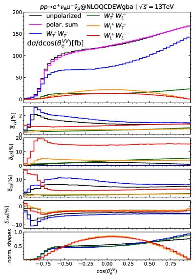
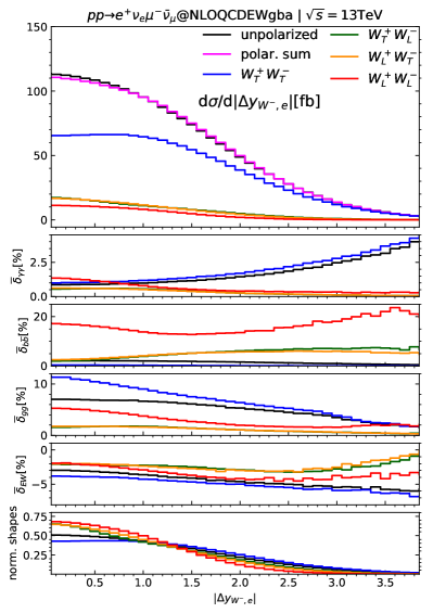
Figure 3: Distributions in $\cos\theta^{VV}_{e}$ (left) and $|y_{e^{+}}-y_{W^{-}}|$ (right). The big panel shows the absolute values of the cross sections including all contributions from the $q\bar{q}$, $gg$, $b\bar{b}$, $\gamma\gamma$ processes. The middle panels display the corrections with respect to the NLO QCD $q\bar{q}$ cross sections. The bottom panel shows the normalized shapes of the distributions plotted in the top panel.

It is found that the EW corrections are mostly negative with the largest magnitude of around $10\%$ occurring in the TT polarization at $\cos(\theta_{e}^{\text{VV}})\approx-0.9$. For the $b\bar{b}$ correction to the LL polarization, we see that it is consistently large over almost the entire phase space. It is interesting to observe that photon-photon correction to the TT mode is increasing with large rapidity separation $|\Delta y_{W^{-},e}|$, while the exact opposite behavior is seen for the gluon-gluon correction. The results show that the $gg$, $b\bar{b}$, $\gamma\gamma$ processes contribute differently to different polarization modes across different regions of the phase space.

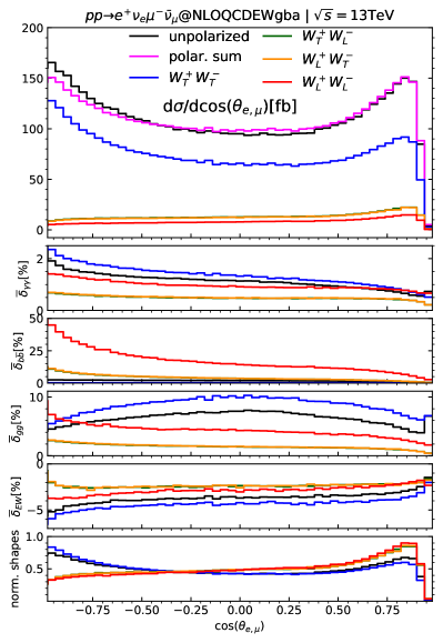
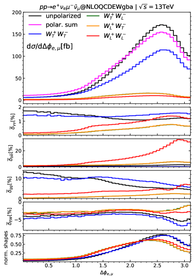
Figure 4: Same as Fig. 3 but for $\cos(\theta_{e,\mu})$ (left) and $\Delta\Phi_{e,\mu}$ (right) distributions.

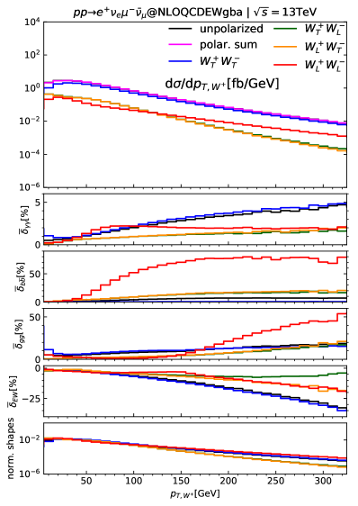
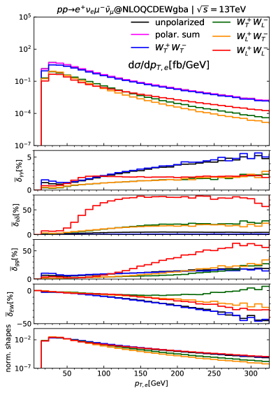
Figure 5: Same as Fig. 3 but for $p_{T,W^{+}}$ (left) and $p_{T,e^{+}}$ (right) distributions.

In similar style, the distributions in $\cos(\theta_{e,\mu})$ with $\theta_{e,\mu}$ being the angle between the positron momentum and the muon momentum and in the azimuthal-angle separation $\Delta\Phi_{e,\mu}$ are plotted in Fig. 4. The EW corrections are all negative, ranging from $-7\%$ to $-1\%$ for all polarization modes. The $b\bar{b}$ correction can reach up to $+45\%$ at $\theta_{e,\mu}=\pi$ and up to $+35\%$ when $\Delta\Phi_{e,\mu}\approx\pi$.

Finally, we present two transverse momentum distributions for the $W^{+}$ and the positron in Fig. 5. At large $p_{T}$, the EW corrections are negative and large for $W^{+}_{T}W^{-}_{T}$, $W^{+}_{L}W^{-}_{L}$, $W^{+}_{L}W^{-}_{T}$ modes, while being very small for the $W^{+}_{T}W^{-}_{L}$ (green line). The difference behavior between the $W^{+}_{L}W^{-}_{T}$ and $W^{+}_{T}W^{-}_{L}$ modes is because we are looking here at the $W^{+}$ boson. If we consider the $p_{T,W^{-}}$ or $p_{T,\mu}$ distributions (not shown here) then the EW corrections are smallest for the $W^{+}_{L}W^{-}_{T}$ mode. It is interesting to notice that the EW corrections are largest for the TT mode. In this high $p_{T}$ region, it is also important to note that contributions from the $b\bar{b}$ and $gg$ processes are large for the LL mode.

6 Conclusions

In this paper NLO EW corrections to the doubly-polarized cross sections of the $W^{+}W^{-}$ production process at the LHC have been presented. The calculation is based on the method provided in our previous work for the $W^{\pm}Z$ processes Le:2022ppa . Two new ingredients are needed to complete the dipole subtraction terms, one related to the final-state emitter final-state spectator contribution for the photon-radiated process and the other related to the photon-photon induced contribution to the quark-photon induced process. They do not occur in the $WZ$ process because there is only one charged gauge boson in the final state. The calculation of these new terms is straightforward following the guidelines of Le:2022ppa . All details are provided in the appendix.

Numerical results have been provided for the leptonic $e^{+}\nu_{e}\mu^{-}\bar{\nu}_{\mu}$ final state using a realistic fiducial cut setup inspired from an ATLAS analysis. We found that, in the large $p_{T}$ region, the EW corrections are largest (in absolute value) for the TT polarization mode.

Besides the main results for the NLO EW corrections, we have also calculated the subleading contributions from the $gg$, $b\bar{b}$, $\gamma\gamma$ processes. It was found that the $b\bar{b}$ contribution is important for the LL mode, amounting to $15\%$ for the LL integrated cross section, and can be much larger for differential cross sections in some regions of the phase space. This effect comes from the heavy top quark.

Note added:

When we are at the final stage of completing this manuscript, the paper Denner:2023ehn performing the same calculation appears. Their numerical results are different from ours because of different kinematic cuts, in particular the absence of a jet veto in their setup. A detailed comparison takes time, hence will be left for future work.

Appendix A New ingredients in NLO EW corrections

As mentioned in Section 3, compared to the $WZ$ calculation described in Le:2022ppa , there are two new ingredients occurring in the $W^{+}W^{-}$ process. They are the final-state emitter and final-state spectator contribution of the OS production part in the dipole-subtraction method and the $\gamma\gamma\to 4\ell$ induced contribution to the quark-photon induced processes occurring at NLO.

Since these calculations are built on the method of Le:2022ppa , we need to repeat here the notation to explain them in detail. The calculation of NLO EW corrections in the DPA is divided into the production and decay parts. The decay part is the same as in the $WZ$ process, hence there is no need to repeat it here. The new ingredients are related to the following amplitudes of the production part

$$\delta\mathcal{A}_{\text{$\gamma$-rad,prod}}^{\bar{q}q\to V_{1}V_{2}\to 4l\gamma} =\frac{1}{Q_{1}Q_{2}}\sum_{\lambda_{1},\lambda_{2}}\delta\mathcal{A}_{\text{$\gamma$-rad,prod}}^{\bar{q}q\to V_{1}V_{2}\gamma}\mathcal{A}_{\text{LO}}^{V_{1}\to\ell_{1}\ell_{2}}\mathcal{A}_{\text{LO}}^{V_{2}\to\ell_{3}\ell_{4}},$$ (6)

$$\delta\mathcal{A}_{\text{$\gamma$-ind,prod}}^{q\gamma\to V_{1}V_{2}q\to 4lq} =\frac{1}{Q_{1}Q_{2}}\sum_{\lambda_{1},\lambda_{2}}\delta\mathcal{A}_{\text{$\gamma$-ind,prod}}^{q\gamma\to V_{1}V_{2}q}\mathcal{A}_{\text{LO}}^{V_{1}\to\ell_{1}\ell_{2}}\mathcal{A}_{\text{LO}}^{V_{2}\to\ell_{3}\ell_{4}},$$ (7)

where the correction amplitudes $\delta\mathcal{A}_{\text{$\gamma$-rad,prod}}^{\bar{q}q\to V_{1}V_{2}\gamma}$ ($\gamma$-radiated) and $\delta\mathcal{A}_{\text{$\gamma$-ind,prod}}^{q\gamma\to V_{1}V_{2}q}$ ($\gamma$-induced) have been calculated in the OS production calculation in Ref. Baglio:2013toa and hence are reused here. The denominators $Q_{j}$ are computed from the off-shell lepton momenta as in Eq. (4).

To calculate the corresponding cross sections, we use the dipole-subtraction method Catani:1996vz ; Dittmaier:1999mb where the differential cross section reads

$$\left(\frac{d\sigma}{d\xi}\right)_{\text{NLO}}= \int d\Phi_{n}^{(4)}\mathcal{B}(\Phi_{n}^{(4)})\delta(\xi-\xi_{n})$$

$$+\int d\Phi_{n}^{(4)}\left[\mathcal{V}(\Phi_{n}^{(D)})+\mathcal{C}(\Phi_{n}^{(D)})+\int d\Phi_{\text{rad}}^{(D)}\mathcal{D}_{\text{int}}(\Phi_{n}^{(D)},\Phi_{\text{rad}}^{(D)})\right]_{D=4}\delta(\xi-\xi_{n})$$

$$+\int d\Phi_{n+1}^{(4)}\left[\mathcal{R}(\Phi_{n+1}^{(4)})\delta(\xi-\xi_{n+1})-\mathcal{D}_{\text{sub}}(\tilde{\Phi}_{n}^{(4)},\Phi_{\text{rad}}^{(4)})\delta(\xi-\tilde{\xi}_{n})\right],$$ (8)

where $\mathcal{B}$ and $\mathcal{V}$ are the Born and virtual contributions.

The amplitudes Eq. (6) and Eq. (7) occur in the $\mathcal{R}$ term in the bottom line of Eq. (8). Since they are singular in the IR (soft and collinear) limits, the idea of the subtraction method is to introduce a subtraction term $\mathcal{D}_{\text{sub}}$ which matches the function $\mathcal{R}$ in the singular limits so that the new integrand $\mathcal{R}-\mathcal{D}_{\text{sub}}$ is integrable. The corresponding integrated part of $\mathcal{D}_{\text{sub}}$ is obviously singular, but all these divergences cancel in the sum with the virtual corrections ($\mathcal{V}$) and the PDF counter terms ($\mathcal{C}$). The $\mathcal{D}_{\text{int}}$ term in the second line of Eq. (8) is a piece of the $\mathcal{D}_{\text{sub}}$ integrated counter part. The tilde mark in the bottom line of Eq. (8) is to indicate Catani-Seymour mappings, which are used to calculate the $n$-particle kinematics from the $(n+1)$-particle kinematics. These mappings are fully provided in Catani:1996vz ; Dittmaier:1999mb ; Dittmaier:2008md . The version of Dittmaier:1999mb (for the $\gamma$-rad) and of Dittmaier:2008md (for the $\gamma$-ind) is used in this work.

The calculation of the $\mathcal{R}$ terms (for both $\gamma$-rad and $\gamma$-ind) follows the same steps as in Le:2022ppa and no complication arises here. We first generate the off-shell momenta $[k_{(n+1)}]$ for the $(n+1)$ process. From this, a set of OS momenta $[\hat{k}_{(n+1)}]$ is computed using an OS mapping as described in Le:2022ppa .

The first new complication arises in the $\mathcal{D}_{\text{sub}}$ term. For this we need to discuss separately the $\gamma$-rad and $\gamma$-ind processes.

The $\mathcal{D}_{\text{sub}}$ term of the $\gamma$-rad process is a sum of so-called dipole terms. Compared to the $WZ$ case, there is a new term called final-state emitter and final-state spectator contribution, which happens because both OS $W$ can radiate photon. We follow the guidelines of Dittmaier:1999mb to calculate this. The subtraction function for the OS production $\bar{q}q\to W^{+}W^{-}\gamma$ reads Dittmaier:1999mb (see Section 4.1 there), denoting the OS momenta here as $[p]$ instead of $[\hat{k}]$ for simplicity, $p_{i}=p_{V_{i}}$, $p_{j}=p_{V_{j}}$, $m_{i}=M_{V_{i}}$, $m_{j}=M_{V_{j}}$ (being the OS $W$ mass here),

$$\mathcal{\hat{D}}_{\text{sub}}^{ij}(p) \sim\hat{g}_{\text{sub}}(p_{i},p_{j},p_{\gamma})\mathcal{\hat{B}}(\tilde{p}_{q},\tilde{p}_{i},\tilde{p}_{j}),$$ (9)

$$\hat{g}_{\text{sub}} =\frac{1}{(p_{i}p_{\gamma})R_{ij}(\hat{y}_{ij})}\left(\frac{2}{1-\hat{z}_{ij}(1-\hat{y}_{ij})}-1-\hat{z}_{ij}-\frac{m_{i}^{2}}{p_{i}p_{\gamma}}\right),$$ (10)

$$\hat{y}_{ij} =\frac{p_{i}p_{\gamma}}{p_{i}p_{j}+p_{i}p_{\gamma}+p_{j}p_{\gamma}},\quad\hat{z}_{ij}=\frac{p_{i}p_{j}}{p_{i}p_{j}+p_{j}p_{\gamma}},$$ (11)

$$\tilde{p}_{j}^{\mu} =\frac{\sqrt{\lambda(P_{ij}^{2},m_{i}^{2},m_{j}^{2})}}{\sqrt{\lambda[(p_{i}+p_{\gamma})^{2},P_{ij}^{2},m_{j}^{2}]}}\big{(}p_{j}^{\mu}-\frac{P_{ij}p_{j}}{P_{ij}^{2}}P_{ij}^{\mu}\big{)}+\frac{P_{ij}^{2}+m_{j}^{2}-m_{i}^{2}}{2P_{ij}^{2}}P_{ij}^{\mu},$$ (12)

$$\tilde{p}_{i}^{\mu} =P_{ij}^{\mu}-\tilde{p}_{j}^{\mu},\quad P_{ij}=p_{i}+p_{j}+p_{\gamma},$$ (13)

where the subscript $i$ denotes a final-state emitter, $j$ a final-state spectator and the remaining quark momenta $[\tilde{p}_{q}]$ are the same as the corresponding quark momenta $[p_{q}]$, and the following auxiliary functions Dittmaier:1999mb

$$\lambda(x,y,z) =x^{2}+y^{2}+z^{2}-2xy-2xz-2yz,$$ (14)

$$R_{ij}(y) =\frac{\sqrt{[2m_{j}^{2}+\bar{P}_{ij}^{2}(1-y)]^{2}-4P_{ij}^{2}m_{j}^{2}}}{\sqrt{\lambda(P_{ij}^{2},m_{i}^{2},m_{j}^{2})}},$$ (15)

with $\bar{P}_{ij}^{2}=P_{ij}^{2}-m_{i}^{2}-m_{j}^{2}$. The factor $\mathcal{\hat{B}}(\tilde{p}_{q},\tilde{p}_{i},\tilde{p}_{j})$ in Eq. (9) is the Born amplitude of the reduced process where the photon has been removed.

Taking into account the leptonic decays using the DPA we have

$$\mathcal{\hat{D}}_{\text{sub}}^{ij}(k)\delta(\xi-\tilde{\xi}_{n}) \sim\hat{g}_{\text{sub}}(\hat{k}_{i},\hat{k}_{j},\hat{k}_{\gamma})\mathcal{B}(\hat{\tilde{k}}_{q},\hat{\tilde{k}}_{i},\hat{\tilde{k}}_{j})\delta(\xi-\tilde{\xi}_{n}),$$ (16)

where the on-shell momenta $[\hat{k}_{(n+1)}]$ are obtained from the off-shell momenta $[k_{(n+1)}]$ using an OS mapping as in Le:2022ppa . We remind that the hat mark is to indicate that the momentum is an OS-mapped quantity. The singular factor $\hat{g}_{\text{sub}}$ is calculated using OS momenta as for the final-state emitter initial-state spectator terms. Notice that it is Lorentz invariant, hence can be calculated in any reference frame. The subtlety comes in the calculation of the reduced Born amplitude. For this, we first need to compute the off-shell momenta $[\tilde{k}_{n}]$ from the off-shell momenta $[k_{(n+1)}]$ using CS mapping. After this step, an OS mapping is used to calculate $[\hat{\tilde{k}}_{n}]$.

The off-shell momenta $[\tilde{k}_{n}]$ are obtained as follows. We first calculate the off-shell momenta $\tilde{k}_{q}$, $\tilde{k}_{V_{1}}$, $\tilde{k}_{V_{2}}$ using Eq. (12) and Eq. (13) with $p_{1}=k_{e}+k_{\nu_{e}}$, $p_{2}=k_{\mu}+k_{\nu_{\mu}}$, $m_{1}^{2}=p_{1}^{2}$, $m_{2}^{2}=p_{2}^{2}$. The corresponding tilde momenta for the leptons $\tilde{k}_{e}$, $\tilde{k}_{\nu_{e}}$ are obtained from $\tilde{k}_{V_{1}}$ using the off-shell mapping described in Le:2022ppa (see Eq. (4.17) there). Similarly, $\tilde{k}_{\mu}$, $\tilde{k}_{\nu_{\mu}}$ are obtained from $\tilde{k}_{V_{2}}$. After this, the same steps as for the final-state emitter and initial-state spectator follow straightforwardly.

We now come to the $\mathcal{D}_{\text{sub}}$ term of the $\gamma$-ind process $q\gamma\to V_{1}V_{2}q$ with subsequent leptonic decays. There are two singular splittings: $\gamma\to q\bar{q}^{*}$ and $q\to q\gamma^{*}$, corresponding to two dipole terms. We follow the method described in Dittmaier:2008md to calculate these dipole terms. The splitting $\gamma\to q\bar{q}^{*}$, treated in Section 3 of Dittmaier:2008md , occurs in the $WZ$ process and is similar to the $g\to q\bar{q}^{*}$ splitting in the NLO QCD case. This calculation has been described in Denner:2021csi ; Le:2022ppa . The new thing here is related to the $q\to q\gamma^{*}$ splitting, followed by $\gamma\gamma\to W^{+}W^{-}$ scattering. For this, we follow Section 5 of Dittmaier:2008md , using the initial-state spectator to calculate the dipole term. Compared to the dipole terms from $W^{*}\to W\gamma$ splitting of the $\gamma$-rad process, the singular factor $g_{\text{sub}}$ (which is called $h_{\kappa_{f},\mu\nu}^{ff,a}$ in Eq. (5.8) of Dittmaier:2008md ) here is calculated from off-shell momenta as the initial-state momenta are not affected by the OS mapping. The flow of the computation reads, denoting the process as

$$q(k_{q})+\gamma(k_{\gamma})\to q(k_{q^{\prime}})+\ell_{1}(k_{\ell_{1}})+\ell_{2}(k_{\ell_{2}})+\ell_{3}(k_{\ell_{3}})+\ell_{4}(k_{\ell_{4}}).$$ (17)

We first calculate the reduced off-shell momenta $[\tilde{k}_{n}]$ from $[k_{(n+1)}]$ using the following CS mapping Dittmaier:2008md :

$$\tilde{k}_{\gamma} =k_{\gamma},\quad\tilde{k}_{\gamma^{\prime}}=xk_{q},\quad\tilde{k}_{\ell_{i}}^{\mu}=\Lambda^{\mu}_{\nu}k_{\ell_{i}}^{\nu},$$ (18)

$$x =\frac{k_{q}k_{\gamma}-k_{q^{\prime}}k_{\gamma}-k_{q}k_{q^{\prime}}}{k_{q}k_{\gamma}},$$ (19)

$$\Lambda^{\mu}_{\nu} =g^{\mu}_{\nu}-\frac{(P+\tilde{P})^{\mu}(P+\tilde{P})_{\nu}}{P^{2}+P\tilde{P}}+\frac{2\tilde{P}^{\mu}P_{\nu}}{P^{2}},$$ (20)

$$P =k_{q}+k_{\gamma}-k_{q^{\prime}},\quad\tilde{P}=\tilde{k}_{\gamma^{\prime}}+k_{\gamma}.$$ (21)

The subtraction function $\mathcal{D}_{\text{sub}}$ is then calculated using Eq. (5.8) of Dittmaier:2008md as usual. A subtlety one must pay attention to is that the singular function $h_{\kappa_{f},\mu\nu}^{ff,a}$ is not Lorentz invariant by itself, hence must be calculated in the same reference frame as the reduced Born amplitudes. Needless to say that these reduced amplitudes must be calculated using the OS-mapped momenta $[\hat{\tilde{k}}_{n}]$ which are obtained from $[\tilde{k}_{n}]$ using a leading-order OS mapping as in Le:2022ppa .

The calculation of the corresponding integrated dipole terms follows straightforwardly as in the $WZ$ case, see the guidelines in Le:2022ppa . All the needed dipole functions are provided in Dittmaier:1999mb (for the $\gamma$-rad case) and in Dittmaier:2008md (the $\gamma$-ind).

- (1) OPAL collaboration, G. Abbiendi et al., production and triple gauge boson couplings at LEP energies up to 183-GeV, Eur. Phys. J. C 8 (1999) 191 [hep-ex/9811028].
- (2) ATLAS collaboration, M. Aaboud et al., Measurement of production cross sections and gauge boson polarisation in collisions at TeV with the ATLAS detector, Eur. Phys. J. C79 (2019) 535 [1902.05759].
- (3) ATLAS collaboration, G. Aad et al., Observation of gauge boson joint-polarisation states in WZ production from pp collisions at s=13 TeV with the ATLAS detector, Phys. Lett. B 843 (2023) 137895 [2211.09435].
- (4) CMS collaboration, A. Tumasyan et al., Measurement of the inclusive and differential WZ production cross sections, polarization angles, and triple gauge couplings in pp collisions at = 13 TeV, JHEP 07 (2022) 032 [2110.11231].
- (5) CMS collaboration, A. M. Sirunyan et al., Measurements of production cross sections of polarized same-sign W boson pairs in association with two jets in proton-proton collisions at 13 TeV, Phys. Lett. B 812 (2021) 136018 [2009.09429].
- (6) ATLAS collaboration, G. Aad et al., Evidence of pair production of longitudinally polarised vector bosons and study of CP properties in events with the ATLAS detector at TeV, 2310.04350.
- (7) A. Denner and G. Pelliccioli, Polarized electroweak bosons in production at the LHC including NLO QCD effects, JHEP 09 (2020) 164 [2006.14867].
- (8) A. Denner and G. Pelliccioli, NLO QCD predictions for doubly-polarized WZ production at the LHC, Phys. Lett. B 814 (2021) 136107 [2010.07149].
- (9) D. N. Le and J. Baglio, Doubly-polarized WZ hadronic cross sections at NLO QCD + EW accuracy, Eur. Phys. J. C 82 (2022) 917 [2203.01470].
- (10) D. N. Le, J. Baglio and T. N. Dao, Doubly-polarized WZ hadronic production at NLO QCD+EW: calculation method and further results, Eur. Phys. J. C 82 (2022) 1103 [2208.09232].
- (11) T. N. Dao and D. N. Le, Enhancing the doubly-longitudinal polarization in production at the LHC, Commun. in Phys. 33 (2023) 223 [2302.03324].
- (12) A. Denner and G. Pelliccioli, NLO EW and QCD corrections to polarized ZZ production in the four-charged-lepton channel at the LHC, JHEP 10 (2021) 097 [2107.06579].
- (13) R. Poncelet and A. Popescu, NNLO QCD study of polarised production at the LHC, JHEP 07 (2021) 023 [2102.13583].
- (14) G. Pelliccioli and G. Zanderighi, Polarised-boson pairs at the LHC with NLOPS accuracy, 2311.05220.
- (15) A. Aeppli, F. Cuypers and G. J. van Oldenborgh, corrections to pair production in and collisions, Phys. Lett. B 314 (1993) 413 [hep-ph/9303236].
- (16) A. Aeppli, G. J. van Oldenborgh and D. Wyler, Unstable particles in one loop calculations, Nucl. Phys. B 428 (1994) 126 [hep-ph/9312212].
- (17) A. Denner, S. Dittmaier, M. Roth and D. Wackeroth, Electroweak radiative corrections to in double pole approximation: The RACOONWW approach, Nucl.Phys. B587 (2000) 67 [hep-ph/0006307].
- (18) S. Catani and M. Seymour, A General algorithm for calculating jet cross-sections in NLO QCD, Nucl.Phys. B485 (1997) 291 [hep-ph/9605323].
- (19) S. Dittmaier, A General approach to photon radiation off fermions, Nucl. Phys. B565 (2000) 69 [hep-ph/9904440].
- (20) G. Watt and R. S. Thorne, Study of Monte Carlo approach to experimental uncertainty propagation with MSTW 2008 PDFs, JHEP 08 (2012) 052 [1205.4024].
- (21) J. Gao and P. Nadolsky, A meta-analysis of parton distribution functions, JHEP 07 (2014) 035 [1401.0013].
- (22) L. A. Harland-Lang, A. D. Martin, P. Motylinski and R. S. Thorne, Parton distributions in the LHC era: MMHT 2014 PDFs, Eur. Phys. J. C75 (2015) 204 [1412.3989].
- (23) NNPDF collaboration, R. D. Ball et al., Parton distributions for the LHC Run II, JHEP 04 (2015) 040 [1410.8849].
- (24) J. Butterworth et al., PDF4LHC recommendations for LHC Run II, J. Phys. G43 (2016) 023001 [1510.03865].
- (25) S. Dulat, T.-J. Hou, J. Gao, M. Guzzi, J. Huston, P. Nadolsky et al., New parton distribution functions from a global analysis of quantum chromodynamics, Phys. Rev. D93 (2016) 033006 [1506.07443].
- (26) D. de Florian, G. F. R. Sborlini and G. Rodrigo, QED corrections to the Altarelli-Parisi splitting functions, Eur. Phys. J. C76 (2016) 282 [1512.00612].
- (27) S. Carrazza, S. Forte, Z. Kassabov, J. I. Latorre and J. Rojo, An Unbiased Hessian Representation for Monte Carlo PDFs, Eur. Phys. J. C75 (2015) 369 [1505.06736].
- (28) A. Manohar, P. Nason, G. P. Salam and G. Zanderighi, How bright is the proton? A precise determination of the photon parton distribution function, Phys. Rev. Lett. 117 (2016) 242002 [1607.04266].
- (29) A. V. Manohar, P. Nason, G. P. Salam and G. Zanderighi, The Photon Content of the Proton, JHEP 12 (2017) 046 [1708.01256].
- (30) A. Buckley, J. Ferrando, S. Lloyd, K. Nordström, B. Page, M. Rüfenacht et al., LHAPDF6: parton density access in the LHC precision era, Eur. Phys. J. C75 (2015) 132 [1412.7420].
- (31) ATLAS collaboration, M. Aaboud et al., Measurement of fiducial and differential production cross-sections at TeV with the ATLAS detector, Eur. Phys. J. C 79 (2019) 884 [1905.04242].
- (32) I. W. Stewart and F. J. Tackmann, Theory Uncertainties for Higgs and Other Searches Using Jet Bins, Phys. Rev. D 85 (2012) 034011 [1107.2117].
- (33) A. Denner, C. Haitz and G. Pelliccioli, NLO EW corrections to polarised production and decay at the LHC, 2311.16031.
- (34) J. Baglio, L. D. Ninh and M. M. Weber, Massive gauge boson pair production at the LHC: a next-to-leading order story, Phys. Rev. D88 (2013) 113005 [1307.4331].
- (35) S. Dittmaier, A. Kabelschacht and T. Kasprzik, Polarized QED splittings of massive fermions and dipole subtraction for non-collinear-safe observables, Nucl. Phys. B 800 (2008) 146 [0802.1405].