Reflected entropy in BCFTs on a black hole background

Abstract

We obtain the reflected entropy for bipartite mixed state configurations involving two disjoint and adjacent subsystems in two dimensional boundary conformal field theories (BCFT₂s) in a black hole background. The bulk dual is described by an AdS₃ black string geometry truncated by a Karch-Randall brane. The entanglement wedge cross section computed for this geometry matches with the reflected entropy obtained for the BCFT₂ verifying the holographic duality. In this context, we also obtain the analogues of the Page curves for the reflected entropy and investigate the behaviour of the Markov gap.

1 Introduction

The black hole information loss problem Hawking:1975vcx ; Hawking:1976ra has greatly aided the understanding of many aspects of the quantum theory of gravity. The paradox arises after the Page time when the fine grained entropy of the Hawking radiation from an evaporating black hole exceeds the coarse-grained entropy which leads to a violation of unitarity. Recently the authors Penington:2019npb ; Almheiri:2019psf ; Almheiri:2019hni ; Almheiri:2019yqk ; Penington:2019kki ; Almheiri:2020cfm proposed a novel island formula motivated by the quantum extremal surface (QES) prescription Faulkner:2013ana ; Engelhardt:2014gca for the fine grained entropy of subsystems in quantum field theories coupled to semi-classical theories of gravity which restores the unitarity and leads to the Page curve Page:1993wv ; Page:1993df ; Page:2013dx . This involves certain disconnected regions termed islands arising at late times in the bulk entanglement wedge for subsystems in radiation baths. The authors in Penington:2019kki ; Almheiri:2019qdq ; Dong:2020uxp ; Kawabata:2021vyo have substantiated the island formula from a gravitational path integral for the Rényi entanglement entropy by considering certain replica wormhole saddles which are dominant at late times.

The doubly holographic description Almheiri:2019hni ; Rozali:2019day ; Chen:2020uac ; Chen:2020hmv ; Deng:2020ent ; Suzuki:2022xwv ; Grimaldi:2022suv ; Geng:2020qvw ; Geng:2020fxl ; Geng:2021iyq ; Geng:2021mic ; Geng:2021hlu provides a more intuitive understanding of the island formula, where the radiation baths are described by holographic conformal field theories (CFTs). In the double holographic scenario (bulk perspective) a $d$-dimensional CFT coupled to the semi-classical gravity has been described as dual to a $(d+1)$-dimensional gravitational theory. The island formula may then be obtained through the RT prescription Ryu:2006bv ; Ryu:2006ef ; Hubeny:2007xt in the corresponding higher-dimensional bulk perspective. Furthermore the authors in Suzuki:2022xwv observed an equivalence between a CFT coupled to the semi-classical gravity and a boundary conformal field theory (BCFT) through a combination of the AdS/BCFT correspondence Takayanagi:2011zk ; Fujita:2011fp and the braneworld holography Karch:2000ct ; Karch:2000gx . The bulk dual of this BCFT is then described by an AdS_d+1 spacetime truncated by a codimension one end-of-the-world (EOW) brane, which may be identified as the bulk perspective described earlier.

In the context of the Karch-Randall (KR) braneworld with a bulk black hole geometry, a lower dimensional black hole may be induced on the EOW brane if it intersects the horizon. In the lower dimensional effective description, the CFT on the half line serves as a radiation bath for such black hole on the KR brane. Usually the BCFT is defined on a flat background leading to a non gravitating radiation bath in the lower dimensional effective description implying the existence of massive gravitons Geng:2020qvw . Interestingly in this connection the authors in Geng:2021mic ; Geng:2022dua considered a specific KR braneworld model in which the holographic BCFT_d is defined on an eternal AdS_d black hole background. The bulk dual geometry is then described by an AdS_d+1 black string truncated by a KR brane. In the bulk geometry each AdS_d foliation of the AdS_d+1 black string may support an eternal AdS_d black hole and the asymptotic boundary where the BCFT_d lives is one such eternal AdS_d slice. The authors in Geng:2021mic ; Geng:2022dua computed the EE for the Hawking radiation and obtained the corresponding Page curves.

On a separate note, it is well known in quantum information theory that the EE is not suitable for the characterization of mixed state entanglement. To address this issue several computable mixed state entanglement and correlation measures such as the entanglement negativity Vidal:2002zz ; Plenio:2005cwa ; Calabrese:2012ew ; Calabrese:2012nk ; Calabrese:2014yza , reflected entropy Dutta:2019gen ; Jeong:2019xdr , entanglement of purification Horodecki:EoP ; Takayanagi:2017knl , odd entanglement entropy Tamaoka:2018ned , balance partial entanglement Wen:2021qgx have been proposed in the literature. These measures have also been investigated in the context of the AdS/BCFT scenarios Li:2020ceg ; Li:2021dmf ; Shao:2022gpg ; BasakKumar:2022stg ; Basu:2022reu ; Afrasiar:2022ebi ; Afrasiar:2022fid ; Afrasiar:2023jrj ; Basu:2023wmv ; Kumari:2023ops .

In this article, we focus on one such mixed state correlation measure termed the reflected entropy which involves the canonically purification of the mixed state under consideration and is bounded from below by the mutual information Dutta:2019gen . The holographic reflected entropy was shown to be described by the bulk entanglement wedge cross section (EWCS) Dutta:2019gen . Following this the authors in Hayden:2021gno provided a stricter lower bound in terms of the “Markov gap” given by the difference between the holographic reflected entropy and the mutual information. It was demonstrated that the Markov gap could be interpreted geometrically in terms of the number of non-trivial boundaries of the bulk EWCS. Recently, an island formulation was proposed for the reflected entropy in Chandrasekaran:2020qtn ; Li:2020ceg . Subsequently, the authors in Vardhan:2021mdy ; Akers:2022max have obtained the analogues of the Page curve for the reflected entropy. Although the mixed state entanglement for the Hawking radiation in non-gravitating baths have been studied extensively Li:2020ceg ; Li:2021dmf ; Ling:2021vxe ; Chandrasekaran:2020qtn ; Afrasiar:2022ebi ; Afrasiar:2022fid ; Afrasiar:2023jrj ; Basu:2022reu ; Basu:2023wmv ; KumarBasak:2020ams , the same has not received significant attention for the cases involving a gravitating radiation bath.

In the above context, the investigation of the mixed state entanglement for Hawking radiation in gravitating baths as described in the aforementioned KR braneworld model, is a significant open issue. In the present work, we investigate the same by obtaining the reflected entropy for bipartite mixed states in a BCFT₂ defined on an eternal AdS₂ black hole background which serves as a gravitating radiation bath from the effective lower dimensional perspective. In order to obtain the reflected entropy, first it is required to determine the EE phases for the particular mixed state configuration. Subsequently within each EE phase, we investigate various phases of the reflected entropy upon utilizing the replica technique in the large central charge limit. We also obtain the EWCS in the dual bulk black string geometry, which exactly reproduces the field theory results. Furthermore, we plot the Page curve for the EE and, within each EE phase, investigate the behaviour of the various phases of the reflected entropy with time. We then plot the holographic mutual information for bipartite mixed state configurations in the BCFT₂ and compare the results with the reflected entropy to investigate Markov gap Hayden:2021gno ; Lu:2022cgq .

This article is organized as follows. In section 2, we review some earlier works relevant to our computations. We start with the review of holographic BCFT₂ located on an eternal AdS₂ black hole background described in Geng:2022dua and briefly explain the computation of the EE in this braneworld model. Subsequently, we brief recapitulate the definition of the reflected entropy, Markov gap and their holographic characterization. Following this in section 3 and section 4, we describe the computation of the different possible phases for reflected entropy of bipartite mixed state configurations involving disjoint and adjacent subsystems and their corresponding bulk EWCS for different phases. Furthermore we obtain the Page curve for the reflected entropy and investigate the Markov gap. Finally in section 5 we summarize our results and discuss future directions.

2 Review

In this section we briefly review the salient features of a BCFT₂ on a AdS₂ black hole background described in Geng:2021mic ; Geng:2022dua . We also review the computation of the subregion EE for various two-sided bipartition in this setup. Subsequently we provide the definition of the reflected entropy and the replica technique for its computation in $CFT_{2}s$ and then describe the holographic reflected entropy in terms of the bulk minimal EWCS Takayanagi:2017knl as described in Dutta:2019gen . Furthermore, we also review the issue of the Markov gap Hayden:2021gno described as the difference between the reflected entropy and the holographic mutual information.

2.1 Holographic BCFT₂ in a black hole background

The authors in Geng:2021mic ; Geng:2022dua considered a holographic BCFT₂ on a AdS₂ black hole background. The bulk dual is an AdS₃ black string geometry truncated by a Karch-Randall brane, which is described by the metric

$$ds^{2}=\cosh^{2}\rho\left[-\frac{\left(1-\frac{u}{u_{h}}\right)}{u^{2}}dt^{2}+\frac{du^{2}}{u^{2}\left(1-\frac{u}{u_{h}}\right)}\right]+d\rho^{2},$$ (1)

where $\rho\in[-\infty,\infty]$ and $\rho=-\infty\cup\infty$ is the asymptotic boundary and the KR brane is embedded at a constant $\rho=\rho_{B}$ slice. The accessible bulk region then extends from $\rho=\rho_{B}$ to $\rho=\infty$ as depicted in fig. 1. The geometry on each constant $\rho$ slice of the bulk black string is an eternal AdS₂ black hole which has two asymptotic boundaries. From the AdS₃/BCFT₂ correspondence, the dual field theory is a BCFT₂ on an AdS₂ black hole background with conformal boundary conditions at $u=0$. The bulk geometry may be embedded as a codimension one submanifold in $\mathbb{R}^{2,2}$,

$$ds^{2}=\eta_{AB}dX^{A}dX^{B},\quad\quad\eta_{AB}=\text{diag}(-1,-1,1,1),$$ (2)

with the following embedding equation

$$X_{A}X^{A}=-1.$$ (3)

The metric described by eq. 1 may be obtained by utilizing the following parametrization

$$X_{0}=\frac{2u_{h}-u}{u}\cosh\rho,~{}~{}~{}~{}~{}~{}~{}~{}~{}~{}~{}~{}~{}~{}~{}~{}~{}~{}~{}~{}~{}~{}~{}~{}~{}~{}X_{1}=\frac{2\sqrt{u_{h}^{2}-uu_{h}}}{u}\sinh\frac{2\pi t}{\beta}\cosh\rho,$$

$$X_{2}=\frac{2\sqrt{u_{h}^{2}-uu_{h}}}{u}\cosh\frac{2\pi t}{\beta}\cosh\rho,~{}~{}~{}~{}~{}~{}~{}X_{3}=\sinh\rho,$$ (4)

where $\beta=4\pi u_{h}$ is the inverse Hawking temperature. These embedding coordinates may be utilized to compute the holographic EE for the two sided bipartition in this model Geng:2022dua .

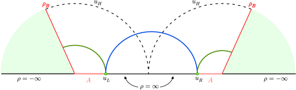
Figure 1: A pictorial representation of the black string geometry. A KR brane is inserted at constant angular coordinate $\rho=\rho_{B}$ shown in red colour. The black string horizon forms the dashed arc at the coordinate $u=u_{h}$. Here we have identified the horizon from both sides of the TFD. The blue curve is a Hartman-Maldacena surface and the green curves are island surfaces. Figure modified from Geng:2022dua

2.2 Entanglement entropy

In this subsection, we will briefly review the computation of the EE between a subsystem $A=(0_{L},u_{L})\cup(0_{R},u_{R})$ and its complement in the above setup both from the field theory and the bulk perspective.

2.2.1 Field theory computation

Utilizing the replica trick, the computation of the EE between the subsystem $A$ and it’s complement is equivalent to computing a two point function of the twist fields $\Phi_{n}$ inserted at the two bipartition points $u_{L}$ and $u_{R}$ as

$$S_{A}=\lim_{n\rightarrow 1}\frac{1}{1-n}\log\langle\Phi_{n}(u_{L},t_{L})\Phi_{n}(u_{R},t_{R})\rangle.$$ (5)

Here for the left bipartition, time coordinate is $t_{L}=t$ while for the right bipartition the time coordinate is given as $\tilde{t}=t_{R}\to-t+\frac{i\beta}{2}$. The metric at the asymptotic boundary of the bulk black string is given as

$$ds^{2}=-\frac{1}{u^{2}}\left(1-\frac{u}{u_{h}}\right)dt^{2}+\frac{du^{2}}{u^{2}\left(1-\frac{u}{u_{h}}\right)}\,,$$ (6)

which is an AdS₂ planar black hole and we have two copies of such geometry corresponding to the two asymptotic boundaries of eq. 1. The BCFT₂ is then located in the AdS₂ black hole background and is not conformally flat, hence the computation of the twist field correlator in eq. 5 is not straightforward. It is necessary to map this field theory on the curved geometry to that on a flat background by using the following series of conformal transformations

$$\omega=u_{h}e^{\frac{u_{\star}+i\tau}{2u_{h}}},\quad u_{\star}=-u_{h}\log\left(1-\frac{u}{u_{h}}\right).$$ (7)

The metric in these new coordinates becomes conformally flat,

$$ds^{2}=4\Omega(u_{\star})^{2}e^{\frac{u_{\star}}{u_{h}}}d\omega d\bar{\omega},$$ (8)

where $\Omega(u_{\star}(u))=\frac{1}{u}\left(1-\frac{u}{u_{h}}\right)$ is the conformal factor. The conformal boundary is then mapped to the circle $\omega\bar{\omega}=u^{2}_{h}$. It is possible to further conformally map this geometry to the upper-half-plane (UHP) through the transformations

$$\omega=\frac{u_{h}}{v-\frac{i}{2}}-iu_{h},$$ (9)

where the conformal boundary is mapped to the real axis $v-\bar{v}=0$ and the metric transforms to

$$ds^{2}=4\Omega(u_{\star})^{2}u^{2}_{h}e^{-\frac{u_{\star}}{u_{H}}}\Big{(}e^{\frac{u_{\star}+i\tau}{2u_{H}}}+i\Big{)}^{2}\Big{(}e^{\frac{{u_{\star}-i\tau}}{2u_{H}}}-i\Big{)}^{2}dvd\bar{v}.$$ (10)

Now, by utilizing the metrics and conformal factor described in eqs. 8 and 10 it is possible to obtain the EE of a subsystem $A$ in the boundary and the bulk channels as Geng:2022dua

$$\text{$S_{A}=\left\{\begin{array}[]{ll}\frac{c}{3}\log\left(\frac{2}{\epsilon}\right)+2\log g_{b}{}&\text{Boundary channel},\\ \frac{c}{6}\log\Bigg{[}\frac{u_{h}}{u_{L}u_{R}}\left(\Delta_{L}+\Delta_{R}+2\sqrt{\Delta_{L}\Delta_{R}}\cosh\frac{t}{u_{h}}\right)\Bigg{]}+\frac{c}{3}\log\left(\frac{2}{\epsilon}\right){}&\text{Bulk channel}.\end{array}\right.$}$$ (11)

where $\log g_{b}\equiv S_{\text{bdy}}$ is the usual boundary entropy in AdS₃/BCFT₂ and $\Delta_{L}=u_{h}-u_{L}$, $\Delta_{R}=u_{h}-u_{R}$ and $\epsilon$ is UV cut-off.

2.2.2 The holographic calculation of EE

On the gravity side, the calculation of the EE for a boundary subsystem $A$ is done by using the Ryu-Takayanagi (RT) formula Ryu:2006bv . In this model, there are two types of RT surfaces: the Island surface, which connects the boundaries of the subsystems to nearby branes, and the Hartman-Maldacena (HM) surface, which passes through the interior of the black string to connect the boundaries of the subsystems. The island and HM surfaces are shown as solid green and blue curves in fig. 1 respectively. In the embedding space formalism, the geodesic length between the points $X^{A}_{1}=(t_{1},u_{1},\rho_{1})$ and $X^{A}_{2}=(t_{2},u_{2},\rho_{2})$ is given as

$$L =\cosh^{-1}\Bigg{[}\left(\frac{(u_{h}+\Delta_{1})(u_{h}+\Delta_{2})-4u_{h}\sqrt{\Delta_{1}\Delta_{2}}\cosh\left(\frac{2\pi(t_{1}-t_{2})}{\beta}\right)}{u_{1}u_{2}}\right)\cosh\rho_{1}\cosh\rho_{2}$$

$$\quad\quad\quad\quad\quad\quad\quad\quad\quad\quad\quad\quad\quad\quad\quad\quad\quad\quad~{}~{}~{}~{}~{}~{}~{}~{}~{}~{}~{}~{}~{}~{}~{}~{}~{}~{}~{}~{}~{}~{}~{}~{}~{}~{}~{}~{}~{}~{}~{}~{}~{}-\sinh\rho_{1}\sinh\rho_{2}\Bigg{]}.$$ (12)

where $\Delta_{1}=u_{h}-u_{1}$ and $\Delta_{2}=u_{h}-u_{2}$.

Length of island surface:

The island surface connects the bipartition points to the nearby branes, shown as solid green curves in fig. 1. In the left copy of thermofield double (TFD) the coordinates of the end points of the island surface are $(u_{L},\rho_{\epsilon},t)$ and $(u_{B},\rho_{B},t)$ where $\rho_{\epsilon}$ describes the regularized asymptotic boundary and $u_{B}$ is a dynamical point on the brane. Now by utilizing these coordinates in section 2.2.2, the length of the island surface may be obtained as

$$L_{\text{Is}}=\log\left[\left(\frac{2u_{h}(\sqrt{\Delta_{L}}-\sqrt{\Delta_{B}})^{2}+u_{L}u_{B}}{u_{L}u_{B}}\right)\cosh\rho_{B}-\sinh\rho_{B}\right]+\rho_{\epsilon}.$$ (13)

The extremal length of the island surface may be obtained by extremizing the above expression over $u_{B}$ as follows

$$L_{\text{Is}}=\rho_{\epsilon}-\rho_{B}.$$ (14)

Finally adding the contribution from the right TFD copy, the EE may be obtained by using RT formula.

Length of the HM surface:

Similar to the previous case, the length of the HM surface may be obtained by utilizing the embedding coordinates of the left and right bipartition in section 2.2.2 as

$$L_{\text{HM}}=\log\left[\frac{e^{2\rho_{\epsilon}}u_{h}}{u_{L}u_{R}}\left(\Delta_{L}+\Delta_{R}+2\sqrt{\Delta_{L}\Delta_{R}}\cosh\frac{t}{u_{h}}\right)\right].$$ (15)

Note that by using the following identifications,

$$\log g_{b}=-\frac{c}{6}\rho_{B}\,,\quad\epsilon=2e^{-\rho_{\epsilon}},$$ (16)

and the Brown-Henneaux formula Brown:1986nw , it can be shown that the field theory results in eq. 11 exactly match with the holographic EE obtained by utilizing eq. 14 and eq. 15. Here the first expression in eq. 16 describes the relation between the boundary entropy $S_{\text{bdy}}$ in AdS₃/BCFT₂ Fujita:2011fp and the brane tension $\rho_{B}$ and the second relation is a matching between the UV and IR cutoffs in the BCFT and the bulk.

2.3 Reflected entropy in CFT₂

In this subsection we briefly review the reflected entropy and its computation in CFT₂ as described in Dutta:2019gen . Let us consider a bipartite quantum system $A\cup B$ in a mixed state $\rho_{AB}$. The canonical purification of this state involves the doubling of its Hilbert space to define a pure state $\ket{\sqrt{\rho_{AB}}}_{ABA^{*}B^{*}}$. The reflected entropy $S_{R}(A:B)$ for the bipartite mixed state is defined as the von Neumann entropy of the reduced density matrix $\rho_{AA^{*}}$ as follows

$$S_{R}(A:B)=S_{vN}(\rho_{AA^{*}})_{\sqrt{\rho_{AB}}}\,\,\,,$$ (17)

where $\rho_{AA^{*}}$ may be obtained by tracing out the degree of freedom of $B$ and $B^{*}$ from the density matrix $\ket{\sqrt{\rho_{AB}}}\bra{\sqrt{\rho_{AB}}}$. The authors in Dutta:2019gen developed a novel replica technique to compute the reflected entropy between two disjoint subsystems $A\equiv[z_{1},z_{2}]$ and $B\equiv[z_{3},z_{4}]$ in a CFT₂. The reflected entropy may then be obtained in terms of a four-point twist field correlator as follows

$$S_{R}(A:B)=\lim_{n,m\to 1}S_{n}(AA^{*})_{\psi_{m}}=\lim_{n,m\to 1}\frac{1}{1-n}\log\frac{\left<\sigma_{g_{A}}(z_{1})\sigma_{g_{A}^{-1}}(z_{2})\sigma_{g_{B}}(z_{3})\sigma_{g_{B}^{-1}}(z_{4})\right>_{\text{CFT}^{\otimes mn}}}{\left<\sigma_{g_{m}}(z_{1})\sigma_{g_{m}^{-1}}(z_{2})\sigma_{g_{m}}(z_{3})\sigma_{g_{m}^{-1}}(z_{4})\right>^{n}_{\text{CFT}^{\otimes m}}}\,,$$ (18)

where $m$, $n$ are the replica indices and twist operators $\sigma_{g_{A}}$ and $\sigma_{g_{B}}$ are inserted at the end points of the subsystems. The conformal dimensions of the operators $\sigma_{g_{A}},\sigma_{g_{B}}$ and $\sigma_{g_{m}}$ are given as Dutta:2019gen

$$h\equiv h_{A}=h_{B}=\frac{nc}{24}\left(m-\frac{1}{m}\right),\quad h_{m}=\frac{c}{24}\left(m-\frac{1}{m}\right),\quad h_{AB}=\frac{2c}{24}\left(n-\frac{1}{n}\right).$$ (19)

It was proved in Dutta:2019gen that the reflected entropy for a bipartite state in a CFT_d in the large central charge limit is dual to twice the minimal EWCS for the bulk static AdS_d+1 geometry. In the next subsection we review the EWCS which describes bulk dual of the reflected entropy.

2.4 Entanglement wedge cross section

The bulk dual of the density matrix $\rho_{AB}$ is described by the entanglement wedge $M_{AB}$ Czech:2012bh which is the region enclosed by the subsystems $A\cup B$ and the codimension two bulk minimal surface $\gamma_{AB}$ homologous to the subsystem $A\cup B$. The entanglement wedge cross section $E_{W}$ is then defined as the minimum cross sectional area of the entanglement wedge Takayanagi:2017knl .

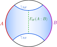
Figure 2: The light green region represents the entanglement wedge and dashed green line is the EWCS of subsystem $A\cup B$.

In the context of AdS₃/CFT₂, the EWCS for two disjoint subsystems $A=[X_{1},X_{2}]$ and $B=[X_{3},X_{4}]$ in terms of the embedding coordinates may be obtained as Kusuki:2019evw

$$E_{W}=\frac{1}{4G_{N}}\cosh^{-1}\left(\frac{1+\sqrt{u}}{\sqrt{v}}\right),$$ (20)

where $u$ and $v$ are defined in terms of $\xi_{ij}=-X_{i}\cdot X_{j}$ as,

$$u=\frac{\xi_{12}\xi_{34}}{\xi_{13}\xi_{24}},\;v=\frac{\xi_{14}\xi_{23}}{\xi_{13}\xi_{24}}.$$ (21)

The length between a point $X_{2}$ and a spacelike geodesic connecting points $X_{1}$, $X_{3}$ may be utilized to obtained the EWCS for two adjacent subsystems as follows

$$E_{W}=\frac{1}{4G_{N}}\cosh^{-1}\left(\sqrt{\frac{2\xi_{12}\xi_{23}}{\xi_{13}}}\right).$$ (22)

The detailed derivation of this formula is described in appendix A.

2.5 Markov gap

In Hayden:2021gno authors have shown that the difference between the holographic reflected entropy and holographic mutual information, termed the Markov gap, may be understood geometrically in terms of the number of non-trivial boundaries of the EWCS. In the context of $AdS_{3}/CFT_{2}$, it was shown that

$$S_{R}(A:B)-I(A:B)\geq\frac{\log(2)\ell_{\text{AdS }}}{2G_{N}}\times(\#\text{ of boundaries of EWCS})+\mathcal{O}\left(\frac{1}{G_{N}}\right).$$ (23)

It has been demonstrated that the Markov gap is bounded by the fidelity of a Markov recovery process related to the purification of the mixed state under consideration. For a perfect Markov recovery process, the Markov gap vanishes.

In the following sections, we first compute the reflected entropy for various bipartite states involving two disjoint and adjacent subsystems in BCFT₂ located on a black hole background. We also explain the computation of the bulk EWCS in the context of the black string geometry which exactly reproduce the field theory results.

3 Holographic reflected entropy: Disjoint subsystems

In this section, we compute the reflected entropy and the bulk EWCS for two disjoint subsystems $A\equiv(u_{L_{1}},u_{L_{2}})\cup(u_{R_{1}},u_{R_{2}})$ and $B\equiv(u_{L_{3}},u_{L_{4}})\cup(u_{R_{3}},u_{R_{4}})$ in the AdS₃/BCFT₂ setup described in section 2.1 where the BCFT₂ is defined on an AdS₂ black hole background. Here we considered $u_{L}$ and $u_{R}$ to be asymmetric. The Rényi reflected entropy in this scenario may then be obtained in terms of the twist field correlators as follows

$$S_{n}(AA^{*})_{\psi_{m}}$$

$$=\log\frac{\langle\sigma_{g_{A}}(u_{L_{1}})\sigma_{g_{A}^{-1}}(u_{L_{2}})\sigma_{g_{B}}(u_{L_{3}})\sigma_{g^{-1}_{B}}(u_{L_{4}})\sigma_{g_{B}}(u_{R_{4}})\sigma_{g_{B}^{-1}}(u_{R_{3}})\sigma_{g_{A}}(u_{R_{2}})\sigma_{g_{A}^{-1}}(u_{R_{1}})\rangle_{\mathrm{BCFT}^{\bigotimes mn}}}{\langle\sigma_{g_{m}}(u_{L_{1}})\sigma_{g_{m}^{-1}}(u_{L_{2}})\sigma_{g_{m}}(u_{L_{3}})\sigma_{g^{-1}_{m}}(u_{L_{4}})\sigma_{g_{m}}(u_{R_{4}})\sigma_{g_{m}^{-1}}(u_{R_{3}})\sigma_{g_{m}}(u_{R_{2}})\sigma_{g_{m}^{-1}}(u_{R_{1}})\rangle^{n}_{\mathrm{BCFT}^{\bigotimes m}}}.$$ (24)

To compute the reflected entropy and the bulk EWCS, it is first required to determine the EE phases for the two disjoint subsystems under consideration. In the following we demonstrate four possible phases of the EE depending on the subsystem size and its location. In what follows we describe the computation of the reflected entropy and the bulk EWCS for these EE phases and show that they match verifying the holographic duality mentioned earlier.

3.1 Entanglement entropy phase 1

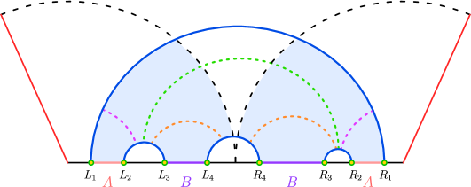
Figure 3: Schematic depicting the different phases of the EWCS (represented by various colored dashed curves) between subsystems $A$ and $B$ when the RT surface for $A\cup B$ is shown by the solid blue curves.

In the first EE phase the subsystems $A\cup B$ are considered to be large and far away from the boundary. Hence the EE for the two disjoint subsystems $A$ and $B$ is proportional to the sum of the lengths of the two HM surfaces corresponding to the points $L_{1}(u_{L_{1}},\rho_{\epsilon},t)$, $R_{1}(u_{R_{1}},\rho_{\epsilon},\tilde{t})$ and $L_{4}(u_{L_{4}},\rho_{\epsilon},t)$, $R_{4}(u_{R_{4}},\rho_{\epsilon},\tilde{t})$ and two dome-type RT surfaces, shown as solid blue curves in fig. 3. Note that $\tilde{t}$ is the time coordinate for the right TFD copy. Now by utilizing section 2.2.2, the geodesic length for the dome-type RT surface connecting points $L_{2}(u_{L_{2}},\rho_{\epsilon},t)$, $L_{3}(u_{L_{3}},\rho_{\epsilon},t)$, may be written as

$$L=\log\left(\frac{u_{h}}{u_{L_{2}}u_{L_{3}}}(\sqrt{\Delta_{L_{2}}}-\sqrt{\Delta_{L_{3}}})^{2}\right)+2\rho_{\epsilon}.$$ (25)

Utilizing eq. 15 and eq. 25 and adding the contribution for the right TFD copy, the EE for this configuration is given as

$$S_{1}= \frac{1}{4G_{N}}\log\left[\frac{u^{2}_{h}\left(\Delta_{L_{1}}+\Delta_{R_{1}}+2\sqrt{\Delta_{L_{1}}\Delta_{R_{1}}}\cosh\frac{t}{u_{h}}\right)\left(\Delta_{L_{4}}+\Delta_{R_{4}}+2\sqrt{\Delta_{L_{4}}\Delta_{R_{4}}}\cosh\frac{t}{u_{h}}\right)}{u_{L_{1}}u_{R_{1}}u_{L_{4}}u_{R_{4}}}\right]$$

$$+\frac{1}{4G_{N}}\log\left[\frac{u^{2}_{h}}{u_{L_{2}}u_{L_{3}}u_{R_{2}}u_{R_{3}}}(\sqrt{\Delta_{L_{2}}}-\sqrt{\Delta_{L_{3}}})^{2}(\sqrt{\Delta_{R_{2}}}-\sqrt{\Delta_{R_{3}}})^{2}\right]+\frac{2\rho_{\epsilon}}{G_{N}}.$$ (26)

For this EE phase, we observe three distinct phases of the reflected entropy and the corresponding bulk EWCS, depicted as dashed curves in fig. 3. Here we consider both the subsystems are far away from the boundary, hence the OPE channel for the BCFT₂ correlator is favoured. In this channel, the BCFT₂ twist field correlators may be expressed as CFT₂ twist field correlators Rozali:2019day ; Li:2021dmf ; Shao:2022gpg . In the following, we describe the computation of the reflected entropy and the bulk EWCS for this EE phase.

Phase-I

Reflected entropy:

In this reflected entropy phase the subsystems are considered to be large and far away from the boundary, hence the numerator of section 3 may be factorized into two two-point twist field correlators and one four-point twist field correlator as

$$\langle\sigma_{g_{A}}(u_{L_{1}})\sigma_{g_{A}^{-1}}(u_{L_{2}})\sigma_{g_{B}}(u_{L_{3}})\sigma_{g^{-1}_{B}}(u_{L_{4}})\sigma_{g_{B}}(u_{R_{4}})\sigma_{g_{B}^{-1}}(u_{R_{3}})\sigma_{g_{A}}(u_{R_{2}})\sigma_{g_{A}^{-1}}(u_{R_{1}})\rangle_{\mathrm{CFT}^{\bigotimes mn}}$$

$$\quad\quad\quad=\langle\sigma_{g_{A}}(u_{L_{1}})\sigma_{g_{A}^{-1}}(u_{R_{1}})\rangle_{\mathrm{CFT}^{\bigotimes mn}}\langle\sigma_{g^{-1}_{B}}(u_{L_{4}})\sigma_{g_{B}}(u_{R_{4}})\rangle_{\mathrm{CFT}^{\bigotimes mn}}$$

$$\quad\quad\quad\quad\quad\quad\quad\quad\quad\times\langle\sigma_{g_{A}^{-1}}(u_{L_{2}})\sigma_{g_{B}}(u_{L_{3}})\sigma_{g_{B}^{-1}}(u_{R_{3}})\sigma_{g_{A}}(u_{R_{2}})\rangle_{\mathrm{CFT}^{\bigotimes mn}}.$$ (27)

The denominator of section 3 may also be factorized similarly. Now by utilizing sections 3 and 3, the reflected entropy in this scenario may be given as

$$S_{R}(A:B)=\lim_{{m,n}\to 1}\frac{1}{1-n}\log\frac{\langle\sigma_{g_{A}^{-1}}(u_{L_{2}})\sigma_{g_{B}}(u_{L_{3}})\sigma_{g_{B}^{-1}}(u_{R_{3}})\sigma_{g_{A}}(u_{R_{2}})\rangle_{\mathrm{CFT}^{\bigotimes mn}}}{\langle\sigma_{g_{m}^{-1}}(u_{L_{2}})\sigma_{g_{m}}(u_{L_{3}})\sigma_{g_{m}^{-1}}(u_{R_{3}})\sigma_{g_{m}}(u_{R_{2}})\rangle^{n}_{\mathrm{CFT}^{\bigotimes m}}}.$$ (28)

Note that the two point twist field correlator in the above expression cancels from the numerator and the denominator. Since the field theory is described on a AdS₂ black hole background, it is necessary to transform the above four-point twist correlator to the flat plane twist field correlator. This transformation is obtained through the conformal map given in eq. 7. Now by utilizing this map and the form of the four point function in the large central charge limit given in Dutta:2019gen ; Fitzpatrick:2014vua , the final expression for the reflected entropy of the two disjoint subsystems may be obtained as

$$S_{R}(A:B)=\frac{c}{6}\log\left[\frac{(1+\sqrt{\eta})(1+\sqrt{\bar{\eta}})}{(1-\sqrt{\eta})(1-\sqrt{\bar{\eta}})}\right],$$ (29)

where the cross ratios $\eta$ and $\bar{\eta}$ are defined as

$$\eta=\frac{\left(\sqrt{\Delta_{L_{2}}}+\sqrt{\Delta_{R_{2}}}e^{t/u_{h}}\right)\left(\sqrt{\Delta_{L_{3}}}+\sqrt{\Delta_{R_{3}}}e^{t/u_{h}}\right)}{\left(\sqrt{\Delta_{L_{2}}}+\sqrt{\Delta_{R_{3}}}e^{t/u_{h}}\right)\left(\sqrt{\Delta_{L_{3}}}+\sqrt{\Delta_{R_{2}}}e^{t/u_{h}}\right)},$$

$$\bar{\eta}=\frac{\left(\sqrt{\Delta_{R_{2}}}+\sqrt{\Delta_{L_{2}}}e^{t/u_{h}}\right)\left(\sqrt{\Delta_{R_{3}}}+\sqrt{\Delta_{L_{3}}}e^{t/u_{h}}\right)}{\left(\sqrt{\Delta_{R_{3}}}+\sqrt{\Delta_{L_{2}}}e^{t/u_{h}}\right)\left(\sqrt{\Delta_{R_{2}}}+\sqrt{\Delta_{L_{3}}}e^{t/u_{h}}\right)}.$$ (30)

EWCS:

The bulk EWCS for this phase is obtained by the length of the geodesic between the two dome-type RT surfaces which is depicted as the dashed green curve in fig. 3. By employing the embedding coordinates provided in section 2.1 for points $L_{2}$, $L_{3}$ and $R_{2}$, $R_{3}$, we may calculate the bulk EWCS using eq. 20, with $u$ and $v$ given as

$$u=\frac{\left(\Delta_{L_{2}}+\Delta_{R_{2}}+2\sqrt{\Delta_{L_{2}}\Delta_{R_{2}}}\cosh\frac{t}{u_{h}}\right)\left(\Delta_{L_{3}}+\Delta_{R_{3}}+2\sqrt{\Delta_{L_{3}}\Delta_{R_{3}}}\cosh\frac{t}{u_{h}}\right)}{\left(\Delta_{L_{2}}+\Delta_{R_{3}}+2\sqrt{\Delta_{L_{2}}\Delta_{R_{3}}}\cosh\frac{t}{u_{h}}\right)\left(\Delta_{L_{3}}+\Delta_{R_{2}}+2\sqrt{\Delta_{L_{3}}\Delta_{R_{2}}}\cosh\frac{t}{u_{h}}\right)},$$

$$v=\frac{\left(\sqrt{\Delta_{L_{2}}}-\sqrt{\Delta_{L_{3}}}\right){}^{2}\left(\sqrt{\Delta_{R_{2}}}-\sqrt{\Delta_{R_{3}}}\right){}^{2}}{\left(\Delta_{L_{2}}+\Delta_{R_{3}}+2\sqrt{\Delta_{L_{2}}\Delta_{R_{3}}}\cosh\frac{t}{u_{h}}\right)\left(\Delta_{L_{3}}+\Delta_{R_{2}}+2\sqrt{\Delta_{L_{3}}\Delta_{R_{2}}}\cosh\frac{t}{u_{h}}\right)}.$$ (31)

Note that the reflected entropy computed in eq. 29 exactly matches with twice the bulk EWCS upon utilizing the Brown-Henneaux relation.

Phase-II

Reflected entropy:

In this reflected entropy phase, we consider the subsystem $A$ to be smaller than $B$, so the numerator in section 3 may be factorized into a two-point and a six-point twist correlator as

$$\langle\sigma_{g_{A}}(u_{L_{1}})\sigma_{g_{A}^{-1}}(u_{L_{2}})\sigma_{g_{B}}(u_{L_{3}})\sigma_{g^{-1}_{B}}(u_{L_{4}})\sigma_{g_{B}}(u_{R_{4}})\sigma_{g_{B}^{-1}}(u_{R_{3}})\sigma_{g_{A}}(u_{R_{2}})\sigma_{g_{A}^{-1}}(u_{R_{1}})\rangle_{\mathrm{CFT}^{\bigotimes mn}}$$

$$=\langle\sigma_{g^{-1}_{B}}(u_{L_{4}})\sigma_{g_{B}}(u_{R_{4}})\rangle_{\mathrm{CFT}^{\bigotimes mn}}\langle\sigma_{g_{A}}(u_{L_{1}})\sigma_{g_{A}^{-1}}(u_{L_{2}})\sigma_{g_{B}}(u_{L_{3}})\sigma_{g_{B}^{-1}}(u_{R_{3}})\sigma_{g_{A}}(u_{R_{2}})\sigma_{g^{-1}_{A}}(u_{R_{1}})\rangle_{\mathrm{CFT}^{\bigotimes mn}}.$$ (32)

Here the six-point function may be expanded in terms of the conformal block $\mathcal{F}_{6}$ which factorizes into a product of two four-point conformal blocks $\mathcal{F}_{4}$ in the OPE channel (which is termed the $\Omega_{1}$ channel in Banerjee:2016qca ) as

$$\mathcal{F}_{6}(u_{L_{1}},u_{L_{2}},u_{L_{3}},u_{R_{3}},u_{R_{2}},u_{R_{1}};h,h_{AB})= \mathcal{F}_{4}(u_{L_{1}},u_{L_{2}},u_{L_{3}},u_{R_{1}};h,h_{AB})$$

$$\times\mathcal{F}_{4}(u_{R_{1}},u_{R_{2}},u_{R_{3}},u_{L_{1}};h,h_{AB}).$$ (33)

The dominant contribution in the above four point conformal block arises from the primary operator $\sigma_{g_{A}g_{B}^{-1}}$ with conformal dimension $h_{AB}$, in the large central charge limit. Now by utilizing sections 3, 3 and 7 and the form of the four point function conformal block in section 3, we may obtain the reflected entropy in this phase as

$$S_{R}(A:B)=\frac{c}{6}\log\left[\frac{(1+\sqrt{\eta})(1+\sqrt{\bar{\eta}})}{(1-\sqrt{\eta})(1-\sqrt{\bar{\eta}})}\right]+\frac{c}{6}\log\left[\frac{(1+\sqrt{\xi})(1+\sqrt{\bar{\xi}})}{(1-\sqrt{\xi})(1-\sqrt{\bar{\xi}})}\right],$$ (34)

where $\eta$, $\bar{\eta}$ and $\xi$, $\bar{\xi}$ are cross ratios. The first two cross ratios $(\eta,\bar{\eta})$ are given as

$$\eta=\frac{\left(\sqrt{\Delta_{L_{1}}}-\sqrt{\Delta_{L_{2}}}\right)\left(\sqrt{\Delta_{L_{3}}}+\sqrt{\Delta_{R_{1}}}e^{t/u_{h}}\right)}{\left(\sqrt{\Delta_{L_{1}}}-\sqrt{\Delta_{L_{3}}}\right)\left(\sqrt{\Delta_{L_{2}}}+\sqrt{\Delta_{R_{1}}}e^{t/u_{h}}\right)},\,\,\bar{\eta}=\frac{\left(\sqrt{\Delta_{L_{1}}}-\sqrt{\Delta_{L_{2}}}\right)\left(\sqrt{\Delta_{R_{1}}}+\sqrt{\Delta_{L_{3}}}e^{t/u_{h}}\right)}{\left(\sqrt{\Delta_{L_{1}}}-\sqrt{\Delta_{L_{3}}}\right)\left(\sqrt{\Delta_{R_{1}}}+\sqrt{\Delta_{L_{2}}}e^{t/u_{h}}\right)}.$$ (35)

The other cross ratios $\xi$ and $\bar{\xi}$ may be obtained by replacing $\Delta_{L_{i}}\longleftrightarrow\Delta_{R_{i}}$ in the expression of cross ratio $\eta$ and $\bar{\eta}$ respectively.

EWCS:

The bulk EWCS may be expressed as the sum of the lengths of the two geodesics which connect a dome-type RT surface to the HM surface on both the TFD copies and depicted as the dashed magenta curves in fig. 3. The length of one of the geodesic may be obtained by employing the embedding coordinates for points $L_{1}$, $L_{2}$, $L_{3}$, and $R_{1}$ in eq. 20, with $u$ and $v$ given as

$$u=\left(\frac{\sqrt{\Delta_{L_{1}}}-\sqrt{\Delta_{L_{2}}}}{\sqrt{\Delta_{L_{1}}}-\sqrt{\Delta_{L_{3}}}}\right)^{2}\left(\frac{\Delta_{L_{3}}+\Delta_{R_{1}}+2\sqrt{\Delta_{L_{3}}\Delta_{R_{1}}}\cosh\frac{t}{u_{h}}}{\Delta_{L_{2}}+\Delta_{R_{1}}+2\sqrt{\Delta_{L_{2}}\Delta_{R_{1}}}\cosh\frac{t}{u_{h}}}\right),$$

$$v=\left(\frac{\sqrt{\Delta_{L_{2}}}-\sqrt{\Delta_{L_{3}}}}{\sqrt{\Delta_{L_{1}}}-\sqrt{\Delta_{L_{3}}}}\right)^{2}\left(\frac{\Delta_{L_{1}}+\Delta_{R_{1}}+2\sqrt{\Delta_{L_{1}}\Delta_{R_{1}}}\cosh\frac{t}{u_{h}}}{\Delta_{L_{2}}+\Delta_{R_{1}}+2\sqrt{\Delta_{L_{2}}\Delta_{R_{1}}}\cosh\frac{t}{u_{h}}}\right).$$ (36)

For the right TFD copy the length of the other geodesic may be obtained by using the embedding coordinates for points $R_{1}$, $R_{2}$, $R_{3}$ and $L_{1}$ in eq. 20. The corresponding ratios $u$ and $v$ may be obtained from section 3 by replacing $\Delta_{L_{i}}\longleftrightarrow\Delta_{R_{i}}$. The final expression for the corresponding bulk EWCS is given by the sum of the lengths of the two geodesics. Upon utilization of the Brown-Henneaux relation, we find that the reflected entropy computed in eq. 34 exactly matches with twice the bulk EWCS.

Phase-III

Reflected entropy:

In this reflected entropy phase, we assume that the subsystem $B$ is smaller than $A$, hence the numerator of section 3 may be factored into a two-point twist correlator and a six-point twist correlator as follows

$$\langle\sigma_{g_{A}}(u_{L_{1}})\sigma_{g_{A}^{-1}}(u_{L_{2}})\sigma_{g_{B}}(u_{L_{3}})\sigma_{g^{-1}_{B}}(u_{L_{4}})\sigma_{g_{B}}(u_{R_{4}})\sigma_{g_{B}^{-1}}(u_{R_{3}})\sigma_{g_{A}}(u_{R_{2}})\sigma_{g_{A}^{-1}}(u_{R_{1}})\rangle_{\mathrm{CFT}^{\bigotimes mn}}$$

$$=\langle\sigma_{g_{A}}(u_{L_{1}})\sigma_{g^{-1}_{A}}(u_{R_{1}})\rangle_{\mathrm{CFT}^{\bigotimes mn}}\langle\sigma_{g^{-1}_{A}}(u_{L_{2}})\sigma_{g_{B}}(u_{L_{3}})\sigma_{g^{-1}_{B}}(u_{L_{4}})\sigma_{g_{B}}(u_{R_{4}})\sigma_{g_{B}^{-1}}(u_{R_{3}})\sigma_{g_{A}}(u_{R_{2}})\rangle_{\mathrm{CFT}^{\bigotimes mn}}$$ (37)

Here, we may expand the six-point function in terms of the conformal block $\mathcal{F}_{6}$, which, in OPE channel, may be factorized as the product of two four-point conformal blocks $\mathcal{F}_{4}$ as detailed in Banerjee:2016qca

$$\mathcal{F}_{6}(u_{L_{2}},u_{L_{3}},u_{L_{4}},u_{R_{4}},u_{R_{3}},u_{R_{2}};h,h_{AB})= \mathcal{F}_{4}(u_{L_{2}},u_{L_{3}},u_{L_{4}},u_{R_{4}};h,h_{AB})$$

$$\times\mathcal{F}_{4}(u_{R_{2}},u_{R_{3}},u_{R_{4}},u_{L_{4}};h,h_{AB}).$$ (38)

Now by utilizing sections 3, 3 and 7 and the conformal block in section 3, we may obtain the expression for the reflected entropy identical to eq. 34 with the cross ratios $\eta,\bar{\eta}$ defined as follows

$$\eta=\frac{\left(\sqrt{\Delta_{L_{2}}}-\sqrt{\Delta_{L_{4}}}\right)\left(\sqrt{\Delta_{L_{3}}}+\sqrt{\Delta_{R_{4}}}e^{t/u_{h}}\right)}{\left(\sqrt{\Delta_{L_{3}}}-\sqrt{\Delta_{L_{4}}}\right)\left(\sqrt{\Delta_{L_{2}}}+\sqrt{\Delta_{R_{4}}}e^{t/u_{h}}\right)},~{}~{}\bar{\eta}=\frac{\left(\sqrt{\Delta_{L_{2}}}-\sqrt{\Delta_{L_{4}}}\right)\left(\sqrt{\Delta_{R_{4}}}+\sqrt{\Delta_{L_{3}}}e^{t/u_{h}}\right)}{\left(\sqrt{\Delta_{L_{3}}}-\sqrt{\Delta_{L_{4}}}\right)\left(\sqrt{\Delta_{R_{4}}}+\sqrt{\Delta_{L_{2}}}e^{t/u_{h}}\right)}.$$ (39)

The other cross ratios $\xi$ and $\bar{\xi}$ may be obtained by replacing $\Delta_{L_{i}}\longleftrightarrow\Delta_{R_{i}}$ in the expression of cross ratio $\eta$ and $\bar{\eta}$ respectively.

EWCS:

The bulk EWCS for this phase is obtained by the sum of the lengths of two geodesics starting from a dome-shaped RT surface and ending at the HM surface, shown as dashed orange curves in the fig. 3. The EWCS in this phase may be obtained by utilizing the embedding coordinates of points $L_{2}$, $L_{3}$, $L_{4}$ and $R_{4}$ in eq. 20 as

$$E_{W}(A:B)= \frac{1}{4G_{N}}\cosh^{-1}\left[\frac{1+\left(\frac{\sqrt{\Delta_{L_{2}}}-\sqrt{\Delta_{L_{4}}}}{\sqrt{\Delta_{L_{3}}}-\sqrt{\Delta_{L_{4}}}}\right)\sqrt{\frac{\Delta_{L_{3}}+\Delta_{R_{4}}+2\sqrt{\Delta_{L_{3}}\Delta_{R_{4}}}\cosh\frac{t}{u_{h}}}{\Delta_{L_{2}}+\Delta_{R_{4}}+2\sqrt{\Delta_{L_{2}}\Delta_{R_{4}}}\cosh\frac{t}{u_{h}}}}}{\left(\frac{\sqrt{\Delta_{L_{2}}}-\sqrt{\Delta_{L_{3}}}}{\sqrt{\Delta_{L_{3}}}-\sqrt{\Delta_{L_{4}}}}\right)\sqrt{\frac{\Delta_{L_{4}}+\Delta_{R_{4}}+2\sqrt{\Delta_{L_{4}}\Delta_{R_{4}}}\cosh\frac{t}{u_{h}}}{\Delta_{L_{2}}+\Delta_{R_{4}}+2\sqrt{\Delta_{L_{2}}\Delta_{R_{4}}}\cosh\frac{t}{u_{h}}}}}\right]$$

$$\qquad\qquad\qquad\qquad\qquad\qquad\qquad\qquad\qquad\qquad\quad+(\Delta_{L_{i}}\longleftrightarrow\Delta_{R_{i}}),$$ (40)

where second term in the preceding equation represents the right TFD contribution in the bulk EWCS. It should be noted that when the Brown-Henneaux relation is used, the above expression of the bulk EWCS matches with half of the reflected entropy computed earlier in this phase.

3.2 Entanglement entropy phase 2

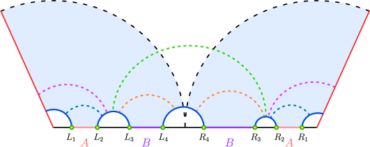
Figure 4: Schematic illustrating the various phases of the EWCS between subsystems A and B (represented by various colored dashed curves), while the RT surface for $A\cup B$ is represented by the solid blue curves.

For this phase, we consider that the subsystem $A$ is close to the boundary while $B$ is far away. So in this case the EE corresponds to the sum of the lengths of the HM surface, two dome-type RT surfaces and two island surfaces shown as blue curves in fig. 4. Now by using eqs. 15, 14 and 25, the EE for this phase may be written as

$$S_{2}= \frac{1}{4G_{N}}\log\left[\frac{u^{2}_{h}}{u_{L_{2}}u_{L_{3}}u_{R_{2}}u_{R_{3}}}(\sqrt{\Delta_{L_{2}}}-\sqrt{\Delta_{L_{3}}})^{2}(\sqrt{\Delta_{R_{2}}}-\sqrt{\Delta_{R_{3}}})^{2}\right]$$

$$+\frac{1}{4G_{N}}\log\left[\frac{u_{h}}{u_{L_{4}}u_{R_{4}}}\left(\Delta_{L_{4}}+\Delta_{R_{4}}+2\sqrt{\Delta_{L_{4}}\Delta_{R_{4}}}\cosh\frac{t}{u_{h}}\right)\right]+\frac{1}{2G_{N}}\left(4\rho_{\epsilon}-\rho_{B}\right).$$ (41)

As seen in fig. 4, this EE phase has four distinctive phases of the reflected entropy or the bulk EWCS. The computation of the reflected entropy and the bulk EWCS for each phase is described in the following subsection.

Phase-I

The reflected entropy or the bulk EWCS in this phase is similar to the first case of the previous EE phase, shown as dashed green curve in fig. 4. Therefore, the reflected entropy is given by eq. 29.

Phase-II

Reflected entropy:

In this reflected entropy phase, we consider that the subsystem $A$ is large enough. Therefore the eight-point twist field correlator in the numerator of section 3 factorizes into two one-point and three two-point twist field correlator in a BCFT₂ as follows

$$\langle\sigma_{g_{A}}(u_{L_{1}})\sigma_{g_{A}^{-1}}(u_{L_{2}})\sigma_{g_{B}}(u_{L_{3}})\sigma_{g^{-1}_{B}}(u_{L_{4}})\sigma_{g_{B}}(u_{R_{4}})\sigma_{g_{B}^{-1}}(u_{R_{3}})\sigma_{g_{A}}(u_{R_{2}})\sigma_{g_{A}^{-1}}(u_{R_{1}})\rangle_{\mathrm{BCFT}^{\bigotimes mn}}$$

$$=\langle\sigma_{g_{A}}(u_{L_{1}})\rangle_{\mathrm{BCFT}^{\bigotimes mn}}\langle\sigma_{g^{-1}_{A}}(u_{R_{1}})\rangle_{\mathrm{BCFT}^{\bigotimes mn}}\langle\sigma_{g^{-1}_{B}}(u_{L_{4}})\sigma_{g_{B}}(u_{R_{4}})\rangle_{\mathrm{BCFT}^{\bigotimes mn}}$$

$$~{}~{}~{}~{}~{}\times\langle\sigma_{g_{A}^{-1}}(u_{L_{2}})\sigma_{g_{B}}(u_{L_{3}})\rangle_{\mathrm{BCFT}^{\bigotimes mn}}\langle\sigma_{g_{A}}(u_{R_{2}})\sigma_{g^{-1}_{B}}(u_{R_{3}})\rangle_{\mathrm{BCFT}^{\bigotimes mn}}.$$ (42)

The first three twist field correlators in the right end side of the above equation cancels with a similar factorization in the denominator of section 3. In order to compute $\langle\sigma_{g_{A}^{-1}}(u_{L_{2}})\sigma_{g_{B}}(u_{L_{3}})\rangle_{\mathrm{BCFT}^{\bigotimes mn}}$ and $\langle\sigma_{g_{A}}(u_{R_{2}})\sigma_{g^{-1}_{B}}(u_{R_{3}})\rangle_{\mathrm{BCFT}^{\bigotimes mn}}$ it is necessary to transform these to the twist field correlators defined on the conformally flat cylindrical background described by the coordinates $(u_{\star},\tau)$ defined in eq. 7. Note that the conformal boundary in these coordinates is located at $u_{\star}=0$. We may now utilize the doubling trick Cardy:2004hm to map these BCFT₂ twist field correlator to the chiral twist field correlator in a CFT₂ defined on the full complex plane, leading to an expression for the reflected entropy as Li:2021dmf

$$S_{R}(A:B)= \lim_{{m,n}\to 1}\frac{1}{1-n}\log\frac{\langle\sigma_{g_{A}}(-u_{\star}({L_{2}}))\sigma_{g_{A}^{-1}}(u_{\star}({L_{2}}))\sigma_{g_{B}}(u_{\star}(u_{L_{3}}))\sigma_{g^{-1}_{B}}(-u_{\star}({L_{3}}))\rangle_{\mathrm{CFT}^{\bigotimes mn}}}{\langle\sigma_{g_{m}}(-u_{\star}({L_{2}}))\sigma_{g_{m}^{-1}}(u_{\star}({L_{2}}))\sigma_{g_{m}}(u_{\star}({L_{3}}))\sigma_{g^{-1}_{m}}(-u_{\star}({L_{3}}))\rangle^{n}_{\mathrm{CFT}^{\bigotimes m}}}$$

$$+ \lim_{{m,n}\to 1}\frac{1}{1-n}\log\frac{\langle\sigma_{g^{-1}_{A}}(-u_{\star}({R_{2}}))\sigma_{g_{A}}(u_{\star}({R_{2}}))\sigma_{g^{-1}_{B}}(u_{\star}({R_{3}}))\sigma_{g_{B}}(-u_{\star}({R_{3}}))\rangle_{\mathrm{CFT}^{\bigotimes mn}}}{\langle\sigma_{g^{-1}_{m}}(-u_{\star}({R_{2}}))\sigma_{g_{m}}(u_{\star}({R_{2}}))\sigma_{g^{-1}_{m}}(u_{\star}({R_{3}}))\sigma_{g_{m}}(-u_{\star}({R_{3}}))\rangle^{n}_{\mathrm{CFT}^{\bigotimes m}}},$$ (43)

where $-u_{\star}$ corresponds to the mirror image of $u_{\star}$. Note that to compute the reflected entropy, it is required to further transform the above four-point twist correlators to the flat plane ($\omega$-plane) twist field correlators. To proceed, we recall that the reflected entropy between two disjoint subsystems $A=[\omega_{1},\omega_{2}]$ and $B=[\omega_{3},\omega_{4}]$ corresponding to the above boundary channel in a BCFT₂ may be obtained in the large central charge limit as Dutta:2019gen ; Fitzpatrick:2014vua ; BasakKumar:2022stg

$$S_{R}(A:B)=\frac{2c}{3}\log\left(\frac{1+\sqrt{1-{\eta}}}{\sqrt{{\eta}}}\right)+2S_{\text{bdy}},$$ (44)

where ${\eta}=\frac{\omega_{23}\omega_{14}}{\omega_{12}\omega_{24}}$ is the cross ratio and the OPE coefficient in the four-point twist field correlator involves the contribution from the boundary entropy as well as the usual OPE coefficient given as Dutta:2019gen ; BasakKumar:2022stg

$$C_{n,m}=e^{2(1-n)S_{\text{bdy}}}(2m)^{-4h}.$$ (45)

Now by utilizing eqs. 44, 45 and 7 in section 3 and accounting for the second term in section 3, the reflected entropy in this phase may be obtained as

$$S_{R}(A:B)=\frac{2c}{3}\log\left(\frac{1+\sqrt{1-\eta}}{\sqrt{\eta}}\right)+\frac{2c}{3}\log\left(\frac{1+\sqrt{1-\xi}}{\sqrt{\xi}}\right)+4S_{\text{bdy}}\,,$$ (46)

where $\eta$ and $\xi$ are the cross ratios on the black hole background defined as

$$\eta=\frac{u_{h}\left(\sqrt{\Delta_{L_{2}}}-\sqrt{\Delta_{L_{3}}}\right)^{2}}{\left(u_{h}-\sqrt{\Delta_{L_{2}}}\sqrt{\Delta_{L_{3}}}\right)^{2}},\quad\quad\xi=\frac{u_{h}\left(\sqrt{\Delta_{R_{2}}}-\sqrt{\Delta_{R_{3}}}\right)^{2}}{\left(u_{h}-\sqrt{\Delta_{R_{2}}}\sqrt{\Delta_{R_{3}}}\right)^{2}}.$$ (47)

EWCS:

The bulk EWCS for this phase is equivalent to the sum of two geodesic lengths which start from the dome-shaped RT surface and end at the EOW brane on both copies of the TFD. These geodesics are shown as dashed magenta curves in the fig. 4. We may now obtain an expression for the length of geodesic which ends on the brane at an arbitrary point $(u_{B},\rho_{B},t)$, by using the embedding coordinates of the points $L_{2}$, $L_{3}$ and $(u_{B},\rho_{B},t)$ in eq. 22 as follows

$$L=\cosh^{-1}\Bigg{[}\frac{1}{u_{B}\sqrt{u_{h}}(\sqrt{\Delta_{L_{2}}}-\sqrt{\Delta_{L_{3}}})} \sqrt{2u_{h}(\sqrt{\Delta_{L_{B}}}-\sqrt{\Delta_{L_{2}}})^{2}\cosh\rho_{B}-u_{L_{2}}u_{B}e^{\rho_{B}}}$$

$$\times\sqrt{2u_{h}(\sqrt{\Delta_{L_{B}}}-\sqrt{\Delta_{L_{3}}})^{2}\cosh\rho_{B}-u_{L_{3}}u_{B}e^{\rho_{B}}}\Bigg{]}.$$ (48)

The bulk EWCS may be computed by extremizing this length over the brane coordinate $u_{B}$. The process of extremizing is complicated in the present scenario, which could be simplified by using a variable change, $u_{i}=u_{h}(1-x_{i}^{2})$. The extremal value of $x_{B}$ is then given as

$$x_{B}=\frac{1+x_{L_{2}}x_{L_{3}}-\sqrt{\left(x^{2}_{L_{2}}-1\right)\left(x^{2}_{L_{3}}-1\right)}}{x_{L_{2}}+x_{L_{3}}}.$$ (49)

Now restoring the $u$ coordinate and using this extremal value in section 3 and adding the contribution from the right TFD copy, the corresponding bulk EWCS in this phase may be obtained as

$$E_{W}(A:B)=\frac{1}{4G_{N}}\Bigg{[} \cosh^{-1}\left(\frac{u_{h}-\sqrt{\Delta_{L_{2}}\Delta_{L_{3}}}}{\sqrt{u_{h}}\left(\sqrt{\Delta_{L_{2}}}-\sqrt{\Delta_{L_{3}}}\right)}\right)$$

$$+\cosh^{-1}\left(\frac{u_{h}-\sqrt{\Delta_{R_{2}}\Delta_{R_{3}}}}{\sqrt{u_{h}}\left(\sqrt{\Delta_{R_{2}}}-\sqrt{\Delta_{R_{3}}}\right)}\right)-2\rho_{B}\Bigg{]}.$$ (50)

Here also using the Brown-Henneaux relation, we find that the reflected entropy computed in eq. 46 exactly matches with twice the bulk EWCS.

Phase-III

Reflected entropy:

In this reflected entropy phase, we consider that the subsystem $A$ is smaller than $B$, hence the numerator of section 3 may be factorized into a two-point and two three-point twist field correlators in the BCFT₂ as follows

$$\langle\sigma_{g_{A}}(u_{L_{1}})\sigma_{g_{A}^{-1}}(u_{L_{2}})\sigma_{g_{B}}(u_{L_{3}})\sigma_{g^{-1}_{B}}(u_{L_{4}})\sigma_{g_{B}}(u_{R_{4}})\sigma_{g_{B}^{-1}}(u_{R_{3}})\sigma_{g_{A}}(u_{R_{2}})\sigma_{g_{A}^{-1}}(u_{R_{1}})\rangle_{\mathrm{BCFT}^{\bigotimes mn}}$$

$$=\langle\sigma_{g^{-1}_{B}}(u_{L_{4}})\sigma_{g_{B}}(u_{R_{4}})\rangle_{\mathrm{BCFT}^{\bigotimes mn}}\langle\sigma_{g_{A}}(u_{L_{1}})\sigma_{g_{A}^{-1}}(u_{L_{2}})\sigma_{g_{B}}(u_{L_{3}})\rangle_{\mathrm{BCFT}^{\bigotimes mn}}$$

$$~{}~{}~{}~{}~{}\times\langle\sigma_{g^{-1}_{A}}(u_{R_{1}})\sigma_{g_{A}}(u_{R_{2}})\sigma_{g^{-1}_{B}}(u_{R_{3}})\rangle_{\mathrm{BCFT}^{\bigotimes mn}}.$$ (51)

The first twist field correlator of the above equation cancels with a similar factorization in the denominator of section 3. To compute $\langle\sigma_{g_{A}}(u_{L_{1}})\sigma_{g_{A}^{-1}}(u_{L_{2}})\sigma_{g_{B}}(u_{L_{3}})\rangle_{\mathrm{BCFT}^{\bigotimes mn}}$ and $\langle\sigma_{g^{-1}_{A}}(u_{R_{1}})\sigma_{g_{A}}(u_{R_{2}})\sigma_{g^{-1}_{B}}(u_{R_{3}})\rangle_{\mathrm{BCFT}^{\bigotimes mn}}$ it is required to transform these to the twist field correlators defined on the conformally flat cylindrical background. Now by using the doubling trick Cardy:2004hm and the similar factorization in the denominator of section 3, we have the following expression of the reflected entropy for two disjoint subsystems as Li:2021dmf

$$S_{R}(A:B)= \lim_{{m,n}\to 1}\frac{1}{1-n}\log\frac{\langle\sigma_{g^{-1}_{A}}(-u_{\star}({L_{1}}))\sigma_{g_{A}}(u_{\star}({L_{1}}))\sigma_{g^{-1}_{A}}(u_{\star}({L_{2}}))\sigma_{g_{B}}(u_{\star}({L_{3}}))\rangle_{\mathrm{CFT}^{\bigotimes mn}}}{\langle\sigma_{g^{-1}_{m}}(-u_{\star}({L_{1}}))\sigma_{g_{m}}(u_{\star}({L_{1}}))\sigma_{g^{-1}_{m}}(u_{\star}({L_{2}}))\sigma_{g_{m}}(u_{\star}({L_{3}}))\rangle^{n}_{\mathrm{CFT}^{\bigotimes m}}}$$

$$+ \lim_{{m,n}\to 1}\frac{1}{1-n}\log\frac{\langle\sigma_{g_{A}}(-u_{\star}({R_{1}}))\sigma_{g^{-1}_{A}}(u_{\star}({R_{1}}))\sigma_{g_{A}}(u_{\star}({R_{2}}))\sigma_{g^{-1}_{B}}(u_{\star}({R_{3}}))\rangle_{\mathrm{CFT}^{\bigotimes mn}}}{\langle\sigma_{g_{m}}(-u_{\star}({R_{1}}))\sigma_{g^{-1}_{m}}(u_{\star}({R_{1}}))\sigma_{g_{m}}(u_{\star}({R_{2}}))\sigma_{g^{-1}_{m}}(u_{\star}({R_{3}}))\rangle^{n}_{\mathrm{CFT}^{\bigotimes m}}}.$$ (52)

Now by utilizing eq. 7 which map these twist field correlators to the flat plane ($\omega$-plane) twist field correlators and the form of the four point conformal block in the large central charge limit Dutta:2019gen ; Fitzpatrick:2014vua , the reflected entropy in this phase may be obtained as

$$S_{R}(A:B)=\frac{c}{3}\log\left[\frac{1+\sqrt{\eta}}{1-\sqrt{\eta}}\right]+\frac{c}{3}\log\left[\frac{1+\sqrt{{\xi}}}{1-\sqrt{{\xi}}}\right],$$ (53)

where $\eta$ and $\xi$ are the cross ratios defined as

$$\eta=\frac{\left(\sqrt{\Delta_{L_{1}}}-\sqrt{\Delta_{L_{2}}}\right)\left(u_{h}-\sqrt{\Delta_{L_{1}}}\sqrt{\Delta_{L_{3}}}\right)}{\left(\sqrt{\Delta_{L_{1}}}-\sqrt{\Delta_{L_{3}}}\right)\left(u_{h}-\sqrt{\Delta_{L_{1}}}\sqrt{\Delta_{L_{2}}}\right)},~{}\xi=\frac{\left(\sqrt{\Delta_{R_{1}}}-\sqrt{\Delta_{R_{2}}}\right)\left(u_{h}-\sqrt{\Delta_{R_{1}}}\sqrt{\Delta_{R_{3}}}\right)}{\left(\sqrt{\Delta_{R_{1}}}-\sqrt{\Delta_{R_{3}}}\right)\left(u_{h}-\sqrt{\Delta_{R_{1}}}\sqrt{\Delta_{R_{2}}}\right)}.$$ (54)

EWCS:

The bulk EWCS for this phase is equivalent to the sum of two geodesic lengths depicted as dashed blue curves in fig. 4. These geodesics connect dome-type RT surface to the island surface on both copies of the TFD. The EWCS may now be calculated by using the embedding coordinates of the three boundary points $L_{1}$, $L_{2}$, $L_{3}$ and one bulk point $(u_{L_{1}},\rho_{B},t)$ in eq. 124 and adding the contribution from the right TFD copy as

$$E_{W}(A:B)=\frac{1}{4G_{N}}\cosh^{-1}\Bigg{[} \frac{\left(\sqrt{\Delta_{L_{1}}}-\sqrt{\Delta_{L_{3}}}\right)\left(u_{h}-\sqrt{\Delta_{L_{1}}\Delta_{L_{2}}}\right)}{u_{L_{1}}\left(\sqrt{\Delta_{L_{2}}}-\sqrt{\Delta_{L_{3}}}\right)}$$

$$+\frac{\left(\sqrt{\Delta_{L_{1}}}-\sqrt{\Delta_{L_{2}}}\right)\left(u_{h}-\sqrt{\Delta_{L_{1}}\Delta_{L_{3}}}\right)}{u_{L_{1}}\left(\sqrt{\Delta_{L_{2}}}-\sqrt{\Delta_{L_{3}}}\right)}\Bigg{]}+~{}(\Delta_{L_{i}}\longrightarrow\Delta_{R_{i}})$$ (55)

Note that when the Brown-Henneaux relation is used, the preceding expression of the bulk EWCS equals half of the reflected entropy calculated in eq. 53.

Phase-IV

The reflected entropy or the bulk EWCS in this phase is similar to the third case of the previous EE phase, shown as dashed orange curves in fig. 4. Therefore, the bulk EWCS is given by section 3.

3.3 Entanglement entropy phase 3

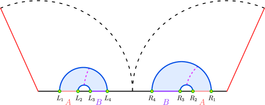
Figure 5: Diagrammatic illustration of the EWCS between subsystems $A$ and $B$ (depicted as dashed curves), where the solid blue curves represent the RT surface for $A\cup B$.

In this EE phase both subsystems are small and located close to one another away from the boundary. Hence the EE for this phase is given by the sum of the lengths of four dome-type RT surfaces, displayed as blue curves in fig. 5. Now, the EE for this phase may be obtained by using eq. 25 as follows

$$S_{3}= \frac{1}{4G_{N}}\log\left[\frac{u^{2}_{h}}{u_{L_{2}}u_{L_{3}}u_{R_{2}}u_{R_{3}}}(\sqrt{\Delta_{L_{2}}}-\sqrt{\Delta_{L_{3}}})^{2}(\sqrt{\Delta_{R_{2}}}-\sqrt{\Delta_{R_{3}}})^{2}\right]$$

$$+\frac{1}{4G_{N}}\log\left[\frac{u^{2}_{h}}{u_{L_{1}}u_{L_{4}}u_{R_{1}}u_{R_{4}}}(\sqrt{\Delta_{L_{1}}}-\sqrt{\Delta_{L_{4}}})^{2}(\sqrt{\Delta_{R_{1}}}-\sqrt{\Delta_{R_{4}}})^{2}\right]+\frac{2\rho_{\epsilon}}{G_{N}}.$$ (56)

For this EE phase we observe only one phase for the reflected entropy or the bulk EWCS shown as dashed magenta curves in fig. 5. Note that here we assume that the subsystems are away from the boundary, hence the OPE channel for the BCFT₂ correlator is favoured.

Reflected entropy:

For the computation of the reflected entropy in this EE phase, the numerator of section 3 may be factorized into two four-point twist field correlators as follows

$$\langle\sigma_{g_{A}}(u_{L_{1}})\sigma_{g_{A}^{-1}}(u_{L_{2}})\sigma_{g_{B}}(u_{L_{3}})\sigma_{g^{-1}_{B}}(u_{L_{4}})\sigma_{g_{B}}(u_{R_{4}})\sigma_{g_{B}^{-1}}(u_{R_{3}})\sigma_{g_{A}}(u_{R_{2}})\sigma_{g_{A}^{-1}}(u_{R_{1}})\rangle_{\mathrm{CFT}^{\bigotimes mn}}$$

$$=\langle\sigma_{g_{A}}(u_{L_{1}})\sigma_{g_{A}^{-1}}(u_{L_{2}})\sigma_{g_{B}}(u_{L_{3}})\sigma_{g^{-1}_{B}}(u_{L_{4}})\rangle_{\mathrm{CFT}^{\bigotimes mn}}\langle\sigma_{g_{B}}(u_{R_{4}})\sigma_{g_{B}^{-1}}(u_{R_{3}})\sigma_{g_{A}}(u_{R_{2}})\sigma_{g_{A}^{-1}}(u_{R_{1}})\rangle_{\mathrm{CFT}^{\bigotimes mn}}.$$ (57)

The denominator of section 3 admits a similar factorization. Hence the reflected entropy in this phase is given as

$$S_{R}(A:B)= \lim_{{m,n}\to 1}\frac{1}{1-n}\log\frac{\langle\sigma_{g_{A}}(u_{L_{1}})\sigma_{g_{A}^{-1}}(u_{L_{2}})\sigma_{g_{B}}(u_{L_{3}})\sigma_{g^{-1}_{B}}(u_{L_{4}})\rangle_{\mathrm{CFT}^{\bigotimes mn}}}{\langle\sigma_{g_{m}}(u_{L_{1}})\sigma_{g_{m}^{-1}}(u_{L_{2}})\sigma_{g_{m}}(u_{L_{3}})\sigma_{g^{-1}_{m}}(u_{L_{4}})\rangle^{n}_{\mathrm{CFT}^{\bigotimes m}}}$$

$$+\lim_{{m,n}\to 1}\frac{1}{1-n}\log\frac{\langle\sigma_{g_{B}}(u_{R_{4}})\sigma_{g_{B}^{-1}}(u_{R_{3}})\sigma_{g_{A}}(u_{R_{2}})\sigma_{g_{A}^{-1}}(u_{R_{1}})\rangle_{\mathrm{CFT}^{\bigotimes mn}}}{\langle\sigma_{g_{m}}(u_{R_{4}})\sigma_{g_{m}^{-1}}(u_{R_{3}})\sigma_{g_{m}}(u_{R_{2}})\sigma_{g_{m}^{-1}}(u_{R_{1}})\rangle^{n}_{\mathrm{CFT}^{\bigotimes m}}}.$$ (58)

Now by utilizing eq. 7 to map these four point twist field correlator to flat plane twist field correlator and then using the form of four point function in the large central charge limit Dutta:2019gen ; Fitzpatrick:2014vua , we may obtain the reflected entropy which is identical to eq. 53 where the cross ratios $\eta$ and $\xi$ are modified to

$$\eta=\frac{\left(\sqrt{\Delta_{L_{1}}}-\sqrt{\Delta_{L_{2}}}\right)\left(\sqrt{\Delta_{L_{3}}}-\sqrt{\Delta_{L_{4}}}\right)}{\left(\sqrt{\Delta_{L_{1}}}-\sqrt{\Delta_{L_{3}}}\right)\left(\sqrt{\Delta_{L_{2}}}-\sqrt{\Delta_{L_{4}}}\right)},~{}\xi=\frac{\left(\sqrt{\Delta_{R_{1}}}-\sqrt{\Delta_{R_{2}}}\right)\left(\sqrt{\Delta_{R_{3}}}-\sqrt{\Delta_{R_{4}}}\right)}{\left(\sqrt{\Delta_{R_{1}}}-\sqrt{\Delta_{R_{3}}}\right)\left(\sqrt{\Delta_{R_{2}}}-\sqrt{\Delta_{R_{4}}}\right)}.$$ (59)

EWCS:

The corresponding EWCS for this phase is proportional to the sum of the lengths of two geodesics shown as dashed magenta curves in fig. 5. Now by utilizing the coordinates of the points $L_{1}$, $L_{2}$, $L_{3}$ and $L_{4}$ in eq. 20 and adding the contribution from the right TFD copy, the bulk EWCS in this case may be obtained as

$$E_{W}(A:B)=\frac{1}{4G_{N}}\log\left[\frac{1+\sqrt{\eta}}{1-\sqrt{\eta}}\right]+\frac{1}{4G_{N}}\log\left[\frac{1+\sqrt{{\xi}}}{1-\sqrt{{\xi}}}\right],$$ (60)

where $\eta$ and $\xi$ are defined in eq. 59. Here also we observe that the above expression for the bulk EWCS is precisely equal to half of the reflected entropy computed earlier upon utilizing the Brown-Henneaux relation.

3.4 Entanglement entropy phase 4

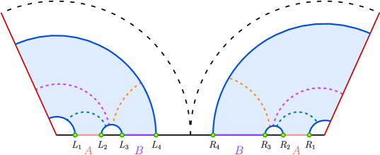
Figure 6: Schematic diagram of the various phases of the EWCS (represented by dashed curves) between subsystems $A$ and $B$ when the RT surface for $A\cup B$ is as depicted by the solid blue curves.

In the last phase we consider that both the subsystems $A$ and $B$ are very close to the boundary, so the boundary channel is dominant. Hence the EE is proportional to sum of the lengths of two dome-type RT surfaces and four island surfaces shown as blue curves in fig. 6. The EE in this configuration may be obtained by using eqs. 14 and 25 as

$$S_{4}=\frac{1}{4G_{N}}\log\left[\frac{u^{2}_{h}}{u_{L_{2}}u_{L_{3}}u_{R_{2}}u_{R_{3}}}(\sqrt{\Delta_{L_{2}}}-\sqrt{\Delta_{L_{3}}})^{2}(\sqrt{\Delta_{R_{2}}}-\sqrt{\Delta_{R_{3}}})^{2}\right]+\frac{1}{G_{N}}\left(2\rho_{\epsilon}-\rho_{B}\right).$$ (61)

In this entropy phase, we observe three different phases for the reflected entropy or the bulk EWCS as shown in fig. 6. We will explain the computation of the reflected entropy and the bulk EWCS phases in the following subsections.

Phase-I

The reflected entropy or the bulk EWCS in this phase is similar to the second case of section 3.2, shown as dashed magenta curves in fig. 6. Therefore, the bulk EWCS is given by section 3.

Phase-II

Reflected entropy:

In this reflected entropy phase we consider the subsystem $B$ to be smaller than $A$, hence the eight-point twist field correlator in the numerator of section 3 factorizes into two one-point and two three-point twist field correlator in BCFT₂ as follows

$$\langle\sigma_{g_{A}}(u_{L_{1}})\sigma_{g_{A}^{-1}}(u_{L_{2}})\sigma_{g_{B}}(u_{L_{3}})\sigma_{g^{-1}_{B}}(u_{L_{4}})\sigma_{g_{B}}(u_{R_{4}})\sigma_{g_{B}^{-1}}(u_{R_{3}})\sigma_{g_{A}}(u_{R_{2}})\sigma_{g_{A}^{-1}}(u_{R_{1}})\rangle_{\mathrm{BCFT}^{\bigotimes mn}}$$

$$=\langle\sigma_{g_{A}}(u_{L_{1}})\rangle_{\mathrm{BCFT}^{\bigotimes mn}}\langle\sigma_{g^{-1}_{A}}(u_{R_{1}})\rangle_{\mathrm{BCFT}^{\bigotimes mn}}\langle\sigma_{g_{A}^{-1}}(u_{L_{2}})\sigma_{g_{B}}(u_{L_{3}})\sigma_{g^{-1}_{B}}(u_{L_{4}})\rangle_{\mathrm{BCFT}^{\bigotimes mn}}$$

$$~{}~{}~{}~{}~{}\times\langle\sigma_{g_{A}}(u_{R_{2}})\sigma_{g^{-1}_{B}}(u_{R_{3}})\sigma_{g_{B}}(u_{R_{4}})\rangle_{\mathrm{BCFT}^{\bigotimes mn}}.$$ (62)

The first two twist field correlators of the preceding expression cancels with a similar factorization in the denominator of section 3. To compute $\langle\sigma_{g_{A}^{-1}}(u_{L_{2}})\sigma_{g_{B}}(u_{L_{3}})\sigma_{g^{-1}_{B}}(u_{L_{4}})\rangle_{\mathrm{BCFT}^{\bigotimes mn}}$ and $\langle\sigma_{g_{A}}(u_{R_{2}})\sigma_{g^{-1}_{B}}(u_{R_{3}})\sigma_{g_{B}}(u_{R_{4}})\rangle_{\mathrm{BCFT}^{\bigotimes mn}}$ we need to transform these to the twist field correlators defined on the conformally flat cylindrical background. Now using the doubling trick Cardy:2004hm and similar factorization in the denominator of section 3, the final expression for the reflected entropy in this case may be written as Li:2021dmf

$$S_{R}(A:B)= \lim_{{m,n}\to 1}\frac{1}{1-n}\log\frac{\langle\sigma_{g^{-1}_{A}}(u_{\star}({L_{2}}))\sigma_{g_{B}}(u_{\star}({L_{3}}))\sigma_{g^{-1}_{B}}(u_{\star}({L_{4}}))\sigma_{g_{B}}(-u_{\star}({L_{4}}))\rangle_{\mathrm{CFT}^{\bigotimes mn}}}{\langle\sigma_{g^{-1}_{m}}(u_{\star}({L_{2}}))\sigma_{g_{m}}(u_{\star}({L_{3}}))\sigma_{g^{-1}_{m}}(u_{\star}({L_{4}}))\sigma_{g_{m}}(-u_{\star}({L_{4}}))\rangle^{n}_{\mathrm{CFT}^{\bigotimes m}}}$$

$$+ \lim_{{m,n}\to 1}\frac{1}{1-n}\log\frac{\langle\sigma_{g_{A}}(u_{\star}({R_{2}}))\sigma_{g^{-1}_{B}}(u_{\star}({R_{3}}))\sigma_{g_{B}}(u_{\star}({R_{4}}))\sigma_{g^{-1}_{B}}(-u_{\star}({R_{4}}))\rangle_{\mathrm{CFT}^{\bigotimes mn}}}{\langle\sigma_{g_{m}}(-u_{\star}({R_{2}}))\sigma_{g^{-1}_{m}}(u_{\star}({R_{3}}))\sigma_{g_{m}}(u_{\star}({R_{4}}))\sigma_{g^{-1}_{m}}(-u_{\star}({R_{4}}))\rangle^{n}_{\mathrm{CFT}^{\bigotimes m}}}.$$ (63)

Now by utilizing eq. 7 and the form of the four point twist field correlator in the large central charge, we may obtain the reflected entropy for two disjoint subsystems which is identical to the expression given in eq. 53 with the cross ratios defined as follows

$$\eta=\frac{\left(\sqrt{\Delta_{L_{3}}}-\sqrt{\Delta_{L_{4}}}\right)\left(u_{h}-\sqrt{\Delta_{L_{2}}\Delta_{L_{4}}}\right)}{\left(\sqrt{\Delta_{L_{2}}}-\sqrt{\Delta_{L_{4}}}\right)\left(u_{h}-\sqrt{\Delta_{L_{3}}\Delta_{L_{4}}}\right)},~{}\xi=\frac{\left(\sqrt{\Delta_{R_{3}}}-\sqrt{\Delta_{R_{4}}}\right)\left(u_{h}-\sqrt{\Delta_{R_{2}}\Delta_{R_{4}}}\right)}{\left(\sqrt{\Delta_{R_{2}}}-\sqrt{\Delta_{R_{4}}}\right)\left(u_{h}-\sqrt{\Delta_{R_{3}}\Delta_{R_{4}}}\right)}.$$ (64)

EWCS:

The bulk EWCS for this phase is the sum of the lengths of two geodesics which connect dome-type RT surface to the island surface on both the TFD copies. These geodesics are shown as dashed orange curves in fig. 6. The bulk EWCS may be obtained by utilizing the coordinates of the three boundary points $L_{2}$, $L_{3}$, $L_{4}$ and one bulk point $(u_{L_{4}},\rho_{B},t)$ in eq. 124 and adding the contribution from the right TFD copy as follows

$$E_{W}(A:B)=\frac{1}{4G_{N}}\cosh^{-1}\Bigg{[} \frac{\left(\sqrt{\Delta_{L_{3}}}-\sqrt{\Delta_{L_{4}}}\right)\left(u_{h}-\sqrt{\Delta_{L_{2}}\Delta_{L_{4}}}\right)}{u_{L_{4}}\left(\sqrt{\Delta_{L_{2}}}-\sqrt{\Delta_{L_{3}}}\right)}$$

$$+\frac{\left(\sqrt{\Delta_{L_{2}}}-\sqrt{\Delta_{L_{4}}}\right)\left(u_{h}-\sqrt{\Delta_{L_{3}}\Delta_{L_{4}}}\right)}{u_{L_{4}}\left(\sqrt{\Delta_{L_{2}}}-\sqrt{\Delta_{L_{3}}}\right)}\Bigg{]}+~{}(\Delta_{L_{i}}\longrightarrow\Delta_{R_{i}}).$$ (65)

Here also using the Brown-Henneaux relation, we notice that the reflected entropy computed earlier precisely matches with twice the bulk EWCS.

Phase-III

The reflected entropy or the bulk EWCS in this phase is similar to the third case of section 3.2, shown as dashed blue curves in fig. 6. Therefore, the bulk EWCS is given by section 3.

3.5 Page curve

In this subsection, we describe the Page curves for the reflected entropy for two disjoint subsystems in a BCFT₂ on an AdS₂ black hole background. To plot the analogue of the Page curve for the reflected entropy, it is necessary to determine the phase transitions in the EE. Within each EE phase, we observe various phases for the reflected entropy depending on the subsystem sizes and their locations.

3.5.1 Case-I

The EE phase transition between phase-2 and phase-4 occurs for a small brane angle and the subsystem $B$ far away from the boundary as shown in fig. 7(a). The Page time $T^{\text{disj}}_{{2\rightarrow 4}}$ for this transition is given as

$$T^{\text{disj}}_{{2\rightarrow 4}}=u_{h}\cosh^{-1}\left(\frac{u^{2}_{h}-u_{h}\left(e^{2\rho_{B}}+1\right)(\Delta_{L_{4}}+\Delta_{R_{4}})+\Delta_{L_{4}}\Delta_{R_{4}}}{2u_{h}e^{2\rho_{B}}\sqrt{\Delta_{L_{4}}\Delta_{R_{4}}}}\right).$$ (66)

From the Page curve of the reflected entropy we observe that in the EE phase-2 the reflected entropy increases initially as the bulk EWCS is the HM surface which grows over time and then remains constant until the Page time as the bulk EWCS lands on the EOW brane. After the Page time eq. 66 the reflected entropy saturates to another smaller constant value in the EE phase-4 as depicted in fig. 7(b). The Page curve for the reflected entropy indicates that before the Page time $T^{\text{disj}}_{{2\rightarrow 4}}$, the Markov gap is always greater than or equal to the anticipated lower bound $\frac{2c}{3}\log{2}$ which is in conformity with eq. 23 because the bulk EWCS phases have two non-trivial boundaries. Additionally, after the Page time $T^{\text{disj}}_{{2\rightarrow 4}}$, since there are four non-trivial boundaries of the bulk EWCS, this gap increases to a value larger than $\frac{4c}{3}\log{2}$.

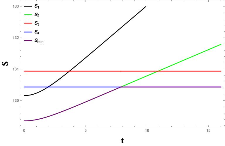
((a))

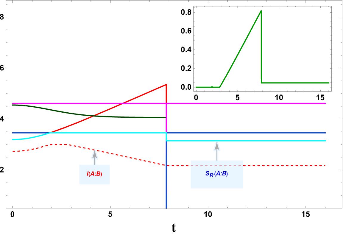
((b))

Figure 7: (a) Page curve of the EE for subsystems $A\cup B$. Here purple curve shows the minimum EE among all the phases. (b) Page curve of the reflected entropy between subsystems $A$ and $B$. Here cyan curve represents minimum $S_{R}$ and red dashed curve is mutual information. (Both graphs are in units of $c$). The inset plot shows the deviation from saturation of the Markov gap eq. 23. The Page curves for the EE and $S_{R}$ is obtained with $u_{h}=1,\Delta_{L_{1}}=0.89,\Delta_{L_{2}}=0.109,\Delta_{L_{3}}=0.102,\Delta_{L_{4}}=5\times 10^{-4},\Delta_{R_{1}}=0.79,\Delta_{R_{2}}=0.109,\Delta_{R_{3}}=0.102,\Delta_{R_{4}}=4\times 10^{-4},\rho_{B}=-0.075,\rho_{\epsilon}=100$.

3.5.2 Case-II

The EE transition between phase-2 and phase-3 may be obtained by considering the subsystem $B$ to be far away from the boundary with the brane angle relatively larger than the one described in the previous case. This EE phase transition is depicted in fig. 8(a) and the Page time $T^{\text{disj}}_{{2\rightarrow 3}}$ is given as follows

$$T^{\text{disj}}_{{2\rightarrow 3}}=u_{h}\cosh^{-1}\left(\frac{u_{h}e^{2\rho_{B}}\left(\sqrt{\Delta_{L_{1}}}-\sqrt{\Delta_{L_{4}}}\right)^{2}\left(\sqrt{\Delta_{R_{1}}}-\sqrt{\Delta_{R_{4}}}\right)^{2}}{2u_{L_{1}}u_{R_{1}}\sqrt{\Delta_{L_{4}}\Delta_{R_{4}}}}-\frac{(\Delta_{L_{4}}+\Delta_{R_{4}})}{2\sqrt{\Delta_{L_{4}}\Delta_{R_{4}}}}\right).$$ (67)

The reflected entropy transition for these EE phases is shown in fig. 8(b). In the EE phase-2, the reflected entropy increases initially as the bulk EWCS is the HM surface and stays constant until $T^{\text{disj}}_{{2\rightarrow 3}}$ as the bulk EWCS lands on the EOW brane and finally after the Page time, it saturates to another constant value in the EE phase-3. From the Page curve of the reflected entropy, as earlier we observe that before the Page time, the Markov gap is always greater than $\frac{2c}{3}\log{2}$, which is consistent with eq. 23 as there are two non-trivial boundaries for the bulk EWCS phases. Additionally, after the Page time, this gap saturates to a value greater than $\frac{4c}{3}\log{2}$ due to the four non-trivial boundaries of the bulk EWCS.

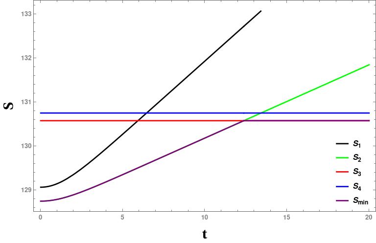
((a))

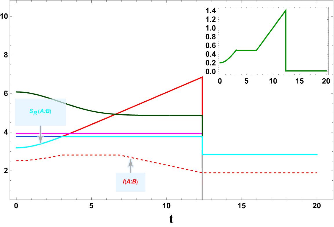
((b))

Figure 8: (a) Page curve of the EE for subsystems $A\cup B$. Here purple curve shows the minimum EE among all the phases. (b) Page curve of the reflected entropy between subsystems $A$ and $B$. Here cyan curve represents minimum $S_{R}$ and red dashed curve is mutual information (All graphs are in units of $c$). The inset plot shows the deviation from saturation of the Markov gap eq. 23. The Page curves for the EE and $S_{R}$ is obtained with $u_{h}=1,\Delta_{L_{1}}=0.69,\Delta_{L_{2}}=0.109,\Delta_{L_{3}}=0.102,\Delta_{L_{4}}=5\times 10^{-6},\Delta_{R_{1}}=0.59,\Delta_{R_{2}}=0.109,\Delta_{R_{3}}=0.102,\Delta_{R_{4}}=4\times 10^{-6},\rho_{B}=-0.55,\rho_{\epsilon}=100$.

3.5.3 Case-III

By implementing a sufficiently larger brane angle than the previous two cases, it is possible to obtain the EE transition between phase-1 and phase-2 at time $T^{\text{disj}}_{1\rightarrow 2}$ and phase-2 and phase-3 at time $T^{\text{disj}}_{{2\rightarrow 3}}$. Here, we additionally consider that subsystem $B$ is located far away from the boundary. This entropy transition is depicted in fig. 9(a). The Page time $T^{\text{disj}}_{{2\rightarrow 3}}$ is given in eq. 67 and $T^{\text{disj}}_{{1\rightarrow 2}}$ may be written as

$$T^{\text{disj}}_{{1\rightarrow 2}}=u_{h}\cosh^{-1}\left(\frac{u^{2}_{h}-u_{h}\left(e^{2\rho_{B}}+1\right)(\Delta_{L_{1}}+\Delta_{R_{1}})+\Delta_{L_{1}}\Delta_{R_{1}}}{2u_{h}\sqrt{\Delta_{L_{1}}\Delta_{R_{1}}}e^{2\rho_{B}}}\right).$$ (68)

In the EE phase-1, the reflected entropy initially rises and then slowly falls until $T^{\text{disj}}_{{1\rightarrow 2}}$ as the growth rate of the bulk EWCS which lands on the HM surface is lower than that of the HM surface. After $T^{\text{disj}}_{{1\rightarrow 2}}$, in the EE phase-2, it increases again and then remains constant until $T^{\text{disj}}_{{2\rightarrow 3}}$ as the bulk EWCS lands on the RT surface which does not cross the horizon. Finally in the EE phase-3, it saturates to a lesser constant value. This reflected entropy Page curve is shown in fig. 9(b). From the Page curve of the reflected entropy we observe that initially the Markov gap is greater than $\frac{2c}{3}\log{2}$ due to the two non-trivial boundaries of the bulk EWCS and after that it is always greater than $\frac{4c}{3}\log{2}$ as for all the bulk EWCS phases have four non-trivial boundaries which verify the inequality mentioned in eq. 23.

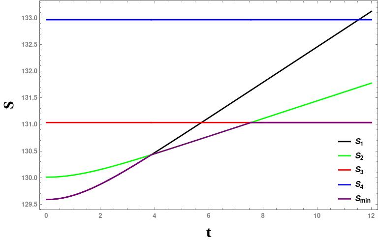
((a))

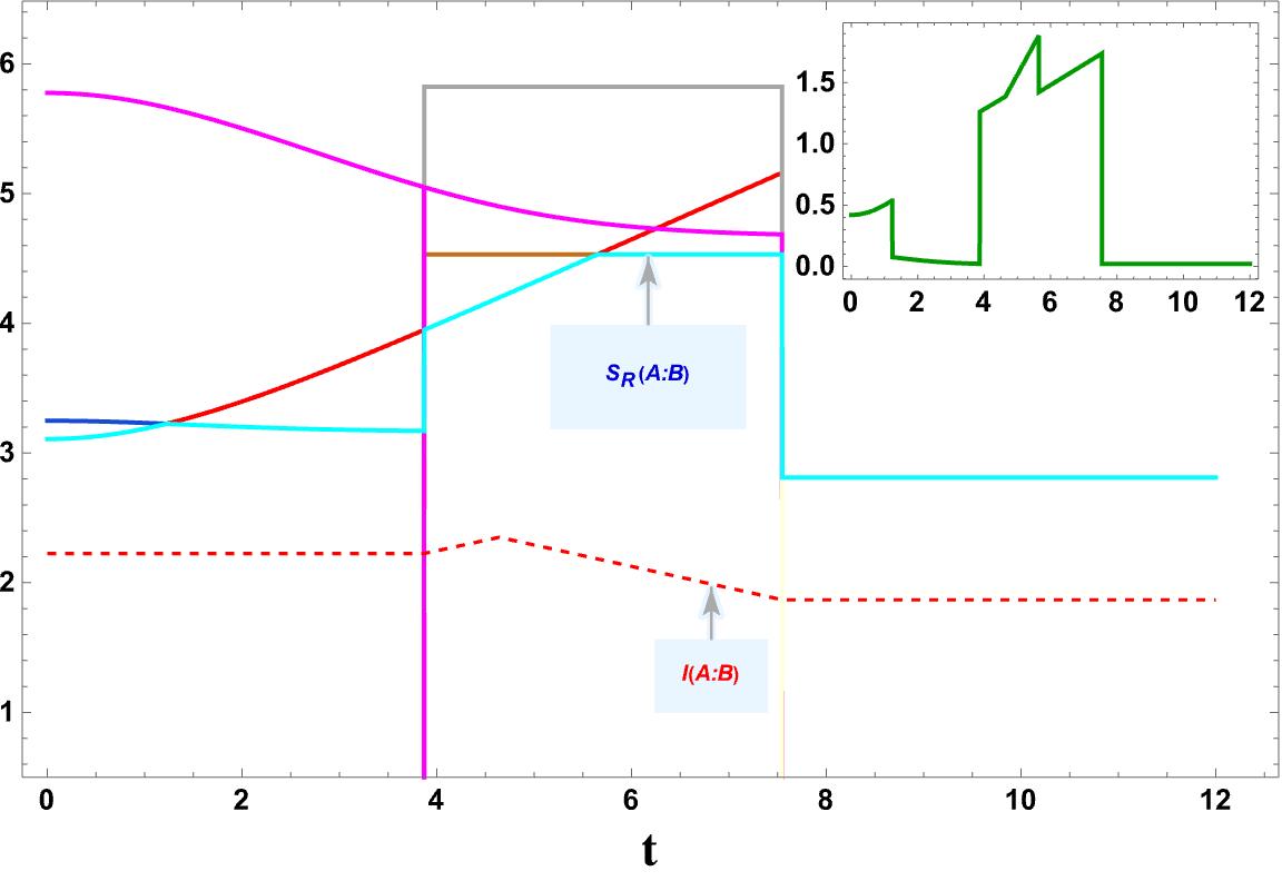
((b))

Figure 9: (a) Page curve of the EE for subsystems $A\cup B$. Here purple curve shows the minimum EE among all the phases. (b) Page curve of the reflected entropy between subsystems $A$ and $B$. Here cyan curve represents minimum $S_{R}$ and red dashed curve is mutual information (All graphs are in units of $c$). The inset plot shows the deviation from saturation of the Markov gap eq. 23. The Page curves for the EE and $S_{R}$ is obtained with $u_{h}=1,\Delta_{L_{1}}=0.89,\Delta_{L_{2}}=0.109,\Delta_{L_{3}}=0.102,\Delta_{L_{4}}=9\times 10^{-6},\Delta_{R_{1}}=0.79,\Delta_{R_{2}}=0.109,\Delta_{R_{3}}=0.1,\Delta_{R_{4}}=8.5\times 10^{-6},\rho_{B}=-3.75,\rho_{\epsilon}=100$.

3.5.4 Case-IV

The EE transition between phase-1 and phase-3 may be obtained by using a relatively large brane angle than first two cases. Here we also take both subsystems away from the boundary. The Page time for this EE phase transition is given as

$$T^{\text{disj}}_{{1\rightarrow 3}}=\cosh^{-1}\left(\frac{\Delta_{L_{1}}+\Delta_{R_{1}}}{\sqrt{\Delta_{L_{1}}\Delta_{R_{1}}}}+\frac{\Delta_{L_{4}}+\Delta_{R_{4}}}{\sqrt{\Delta_{L_{4}}\Delta_{R_{4}}}}-A^{2}\right),$$ (69)

where

$$A^{2}= \left(\frac{\Delta_{L_{1}}}{\Delta_{R_{1}}}+\frac{\Delta_{R_{1}}}{\Delta_{L_{1}}}\right)+\left(\frac{\Delta_{L_{4}}}{\Delta_{R_{4}}}+\frac{\Delta_{R_{4}}}{\Delta_{L_{4}}}\right)-8\Delta_{L_{1}}\Delta_{L_{4}}\Delta_{R_{1}}\Delta_{R_{4}}\left(\frac{\Delta_{L_{1}}+\Delta_{L_{3}}}{\sqrt{\Delta_{L_{1}}\Delta_{L_{4}}}}+\frac{\Delta_{R_{1}}+\Delta_{R_{4}}}{\sqrt{\Delta_{R_{1}}\Delta_{R_{4}}}}\right)$$

$$+20+\frac{2\Delta_{L_{1}}(-\Delta_{L_{4}}+2\Delta_{R_{1}}+\Delta_{R_{4}})+2\Delta_{L_{4}}(\Delta_{R_{1}}+2\Delta_{R_{4}})-2\Delta_{R_{1}}\Delta_{R_{4}}}{\sqrt{\Delta_{L_{1}}\Delta_{L_{4}}\Delta_{R_{1}}\Delta_{R_{4}}}}.$$ (70)

This EE transition and the Page curve of the reflected entropy are depicted in fig. 10(a) and fig. 10(b) respectively. In the EE phase-1 initially the reflected entropy increases with time as the bulk EWCS is the HM surface and then slowly falls until Page time as the growth rate of the bulk EWCS is lesser than the growth rate of the HM surface. After that in the EE phase-3, it saturates to a constant value. The Page curve of the reflected entropy shows that initially the Markov gap is always larger than $\frac{2c}{3}\log{2}$, which agrees with eq. 23, since there are two non-trivial boundaries for the bulk EWCS phase. After that it is always greater than $\frac{4c}{3}\log{2}$ due to the four non-trivial boundaries of the bulk EWCS.

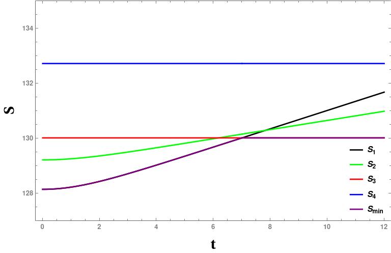
((a))

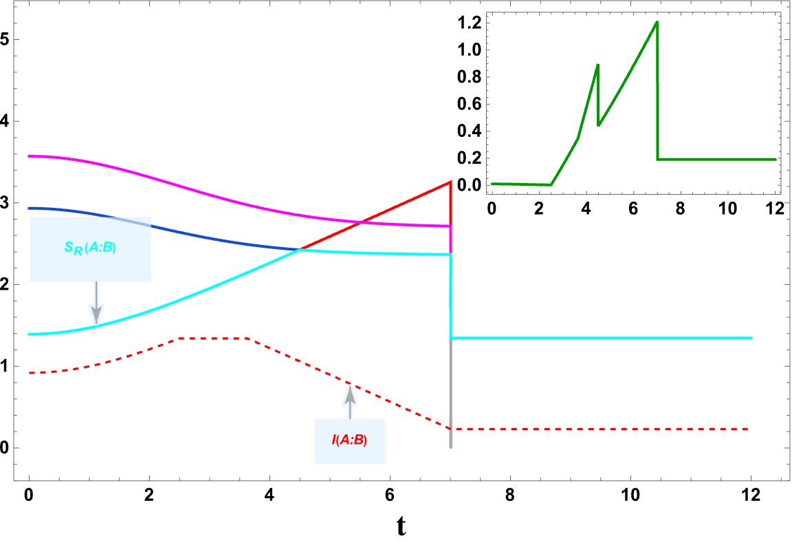
((b))

Figure 10: (a) Page curve of the EE for subsystems $A\cup B$. Here purple curve shows the minimum EE among all the phases. (b) Page curve of the reflected entropy between subsystems $A$ and $B$. Here cyan curve represents minimum $S_{R}$ and red dashed curve is mutual information (All graphs are in units of $c$). The inset plot shows the deviation from saturation of the Markov gap eq. 23. The Page curves for the EE and $S_{R}$ is obtained with $u_{h}=1,\Delta_{L_{1}}=0.3,\Delta_{L_{2}}=9.9\times 10^{-4},\Delta_{L_{3}}=4\times 10^{-4},\Delta_{L_{4}}=2\times 10^{-7},\Delta_{R_{1}}=0.2,\Delta_{R_{2}}=9\times 10^{-4},\Delta_{R_{3}}=3\times 10^{-4},\Delta_{R_{4}}=2\times 10^{-7},\rho_{B}=-3.5,\rho_{\epsilon}=100$.

4 Holographic reflected entropy: Adjacent subsystems

In this section we investigate the computation of the reflected entropy and the bulk EWCS corresponding to two adjacent subsystems $A\equiv(u_{L_{1}},u_{L_{2}})\cup(u_{R_{1}},u_{R_{2}})$ and $B\equiv(u_{L_{2}},u_{L_{3}})\cup(u_{R_{2}},u_{R_{3}})$ in the AdS₃/BCFT₂ setup described in section 2.1 where the BCFT₂ is defined on an AdS₂ black hole background. The Rényi reflected entropy in this scenario is defined in terms of the six-point twist field correlator as

$$S_{n}(AA^{*})_{\psi_{m}}=\frac{1}{1-n}\log\frac{\langle\sigma_{g_{A}}(u_{L_{1}})\sigma_{g_{B}g_{A}^{-1}}(u_{L_{2}})\sigma_{g_{B}^{-1}}(u_{L_{3}})\sigma_{g_{B}}(u_{R_{3}})\sigma_{g_{A}g_{B}^{-1}}(u_{R_{2}})\sigma_{g_{A}^{-1}}(u_{R_{1}})\rangle_{\mathrm{BCFT}^{\bigotimes mn}}}{\langle\sigma_{g_{m}}(u_{L_{1}})\sigma_{g_{m}^{-1}}(u_{L_{3}})\sigma_{g_{m}}(u_{R_{3}})\sigma_{g_{m}^{-1}}(u_{R_{1}})\rangle^{n}_{\mathrm{BCFT}^{\bigotimes m}}}.$$ (71)

Note that for two adjacent subsystems, there are four possible phases of the EE depending on the subsystem size and its location. We will explain the computation of the various reflected entropy phases and the corresponding bulk EWCS for these EE phases in the following subsections.

4.1 Entanglement entropy phase 1

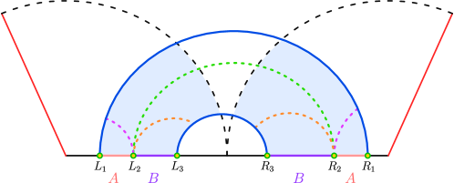
Figure 11: Schematic diagram depicting different phases for the EWCS (shown by different colored dashed curves) between subsystems $A$ and $B$ when the RT surface for $A\cup B$ is as shown by the solid blue curves.

In this EE phase, both subsystems are considered to be large and far away from the boundary. So the EE in this phase is proportional to the lengths of two HM surfaces corresponding to points $L_{1}(u_{L_{1}},\rho_{\epsilon},t)$, $R_{1}(u_{R_{1}},\rho_{\epsilon},\tilde{t})$ and $L_{3}(u_{L_{3}},\rho_{\epsilon},t)$ and $R_{3}(u_{R_{3}},\rho_{\epsilon},\tilde{t})$, depicted as solid blue curves in fig. 11. Now by utilizing eq. 15, we may obtain the EE for this configuration as

$$S_{1}= \frac{1}{4G_{N}}\log\left[\frac{e^{2\rho_{\epsilon}}u_{h}}{u_{L_{1}}u_{R_{1}}}\left(\Delta_{L_{1}}+\Delta_{R_{1}}+2\sqrt{\Delta_{L_{1}}\Delta_{R_{1}}}\cosh\frac{t}{u_{h}}\right)\right]$$

$$+\frac{1}{4G_{N}}\log\left[\frac{e^{2\rho_{\epsilon}}u_{h}}{u_{L_{3}}u_{R_{3}}}\left(\Delta_{L_{3}}+\Delta_{R_{3}}+2\sqrt{\Delta_{L_{3}}\Delta_{R_{3}}}\cosh\frac{t}{u_{h}}\right)\right].$$ (72)

In this EE phase, we observe three possible phases of the reflected entropy or the bulk EWCS, shown as dashed curves in the figure 11. Here we assume that both the subsystems are far away from the boundary, therefore the OPE channel for the BCFT₂ correlator is favoured. In the following, we explain the computation of the reflected entropy and corresponding bulk EWCS for this EE phase.

Phase-I

Reflected entropy:

In this phase we consider that both the subsystems are large and far away from the boundary. Hence, the six-point twist correlator in the numerator of eq. 71 may be factorized into three two-point twist correlators as follows

$$\langle\sigma_{g_{A}}(u_{L_{1}})\sigma_{g_{B}g_{A}^{-1}}(u_{L_{2}})\sigma_{g_{B}^{-1}}(u_{L_{3}})\sigma_{g_{B}}(u_{R_{3}})\sigma_{g_{A}g_{B}^{-1}}(u_{R_{2}})\sigma_{g_{A}^{-1}}(u_{R_{1}})\rangle_{\mathrm{CFT}^{\bigotimes mn}}$$

$$=\langle\sigma_{g_{A}}(u_{L_{1}})\sigma_{g_{A}^{-1}}(u_{R_{1}})\rangle_{\mathrm{CFT}^{\bigotimes mn}}\langle\sigma_{g^{-1}_{B}}(u_{L_{3}})\sigma_{g_{B}}(u_{R_{3}})\rangle_{\mathrm{CFT}^{\bigotimes mn}}$$

$$~{}~{}~{}~{}~{}~{}~{}~{}~{}\times\langle\sigma_{g_{B}g_{A}^{-1}}(u_{L_{2}})\sigma_{g_{A}g_{B}^{-1}}(u_{R_{2}})\rangle_{\mathrm{CFT}^{\bigotimes mn}}.$$ (73)

The twist field correlator in the denominator of eq. 71 admits similar factorization and hence we have the following expression for the reflected entropy between the two adjacent subsystems

$$S_{R}(A:B)=\lim_{{m,n}\to 1}\frac{1}{1-n}\log\langle\sigma_{g_{B}g_{A}^{-1}}(u_{L_{2}})\sigma_{g_{A}g_{B}^{-1}}(u_{R_{2}})\rangle_{\mathrm{CFT}^{\bigotimes mn}}.$$ (74)

Since the field theory is described on a AdS₂ black hole background, therefore the computation of the above twist correlator is not straightforward. But we can map this field theory on the curved geometry to that on a flat background by using the conformal map given in eq. 7. Hence the above twist field correlator may be written as flat plane twist field correlator with an appropriate conformal factor as

$$\langle\sigma_{g_{B}g_{A}^{-1}}(u_{L_{2}})\sigma_{g_{A}g_{B}^{-1}}(u_{R_{2}})\rangle=\frac{4^{-h_{AB}}e^{\frac{u_{*}(u_{L_{2}})h_{AB}}{2u_{h}}}\Omega(u_{L_{2}})^{-h_{AB}}e^{\frac{u_{*}(u_{R_{2}})h_{AB}}{2u_{h}}}\Omega(u_{R_{2}})^{-h_{AB}}\,\epsilon^{2h_{AB}}}{({w_{L_{2}}-w_{R_{2}}})^{2h_{AB}}}\,.$$ (75)

Utilizing eqs. 74, 75 and 19, the reflected entropy in this phase may be obtained as

$$S_{R}(A:B)=\frac{c}{3}\log\left[\frac{4u_{h}}{u_{L_{2}}u_{R_{2}}\epsilon^{2}}\left(\Delta_{L_{2}}+\Delta_{R_{2}}+2\sqrt{\Delta_{L_{2}}\Delta_{R_{2}}}\cosh\frac{t}{u_{h}}\right)\right].$$ (76)

EWCS:

The bulk EWCS for this phase is proportional to the length of the HM surface corresponding to points $L_{2}(u_{L_{2}},\rho_{\epsilon},t)$ and $R_{2}(u_{R_{2}},\rho_{\epsilon},\tilde{t})$, shown as dashed green curve in fig. 11. Now by utilizing eq. 15, the corresponding bulk EWCS may be obtained as

$$E_{W}(A:B)=\frac{1}{4G_{N}}\log\left[\frac{e^{2\rho_{\epsilon}}u_{h}}{u_{L_{2}}u_{R_{2}}}\left(\Delta_{L_{2}}+\Delta_{R_{2}}+2\sqrt{\Delta_{L_{2}}\Delta_{R_{2}}}\cosh\frac{t}{u_{h}}\right)\right].$$ (77)

Note that the above expression for the EWCS matches exactly with half of the reflected entropy computed in eq. 76 upon utilizing eq. 16 and the standard Brown-Henneaux relation in $AdS_{3}/CFT_{2}$.

Phase-II

Reflected entropy:

For this case, consider that the subsystem $A$ is smaller than the subsystem $B$. Therefore, the six points twist correlator in the numerator of eq. 71 may be factorized as one two-point twist correlators and one four-point twist correlator as

$$\langle\sigma_{g_{A}}(u_{L_{1}})\sigma_{g_{B}g_{A}^{-1}}(u_{L_{2}})\sigma_{g_{B}^{-1}}(u_{L_{3}})\sigma_{g_{B}}(u_{R_{3}})\sigma_{g_{A}g_{B}^{-1}}(u_{R_{2}})\sigma_{g_{A}^{-1}}(u_{R_{1}})\rangle_{\mathrm{CFT}^{\bigotimes mn}}$$

$$=\langle\sigma_{g^{-1}_{B}}(u_{L_{3}})\sigma_{g_{B}}(u_{R_{3}})\rangle_{\mathrm{CFT}^{\bigotimes mn}}\langle\sigma_{g_{A}}(u_{L_{1}})\sigma_{g_{B}g_{A}^{-1}}(u_{L_{2}})\sigma_{g_{A}g_{B}^{-1}}(u_{R_{2}})\sigma_{g_{A}^{-1}}(u_{R_{1}})\rangle_{\mathrm{CFT}^{\bigotimes mn}}.$$ (78)

The computation of the four-point twist field correlator in the above expression is not straightforward. It is necessary that the composite twist field $\sigma_{g_{B}g_{A}^{-1}}$ at $u_{L_{2}}$ and $u_{R_{2}}$ may be expanded in terms of twist fields $\sigma_{g_{B}}$ and $\sigma_{g^{-1}_{A}}$. Using this the four-point twist field correlator may be written as

$$\langle\sigma_{g_{A}}(u_{L_{1}})\sigma_{g_{B}g_{A}^{-1}}(u_{L_{2}})\sigma_{g_{A}g_{B}^{-1}}(u_{R_{2}})\sigma_{g_{A}^{-1}}(u_{R_{1}})\rangle_{\mathrm{CFT}^{\bigotimes mn}}$$

$$=\langle\sigma_{g_{A}}(u_{L_{1}})\sigma_{g_{B}}(u_{L_{2}})\sigma_{g^{-1}_{A}}(u^{\prime}_{L_{2}})\sigma_{g_{A}}(u_{R_{2}})\sigma_{g^{-1}_{B}}(u^{\prime}_{R_{2}})\sigma_{g_{A}^{-1}}(u_{R_{1}})\rangle_{\mathrm{CFT}^{\bigotimes mn}},$$ (79)

where we assume that $u^{\prime}_{L_{2}}$ $($$u^{\prime}_{R_{2}})$ are close to $u_{L_{2}}$ ($u_{R_{2}}$). This six-point twist field correlator may now be expanded in terms of two four-point conformal block as described in Banerjee:2016qca . Finally, taking the OPE limit for the for the twist field located at $u_{L_{2}},u^{{}^{\prime}}_{L_{2}}$ and $u_{R_{2}},u^{{}^{\prime}}_{R_{2}}$, the above expression may be written as two three-point twist correlator as follows

$$\langle\sigma_{g_{A}}(u_{L_{1}})\sigma_{g_{B}g_{A}^{-1}}(u_{L_{2}})\sigma_{g_{A}g_{B}^{-1}}(u_{R_{2}})\sigma_{g_{A}^{-1}}(u_{R_{1}})\rangle_{\mathrm{CFT}^{\bigotimes mn}}$$

$$=\langle\sigma_{g_{A}}(u_{L_{1}})\sigma_{g_{B}g_{A}^{-1}}(u_{L_{2}})\sigma_{g_{A}^{-1}}(u_{R_{1}})\rangle_{\mathrm{CFT}^{\bigotimes mn}}\langle\sigma_{g_{A}}(u_{L_{1}})\sigma_{g_{A}g_{B}^{-1}}(u_{R_{2}})\sigma_{g_{A}^{-1}}(u_{R_{1}})\rangle_{\mathrm{CFT}^{\bigotimes mn}}.$$ (80)

The denominator of eq. 71 may be factorized into two two-point twist correlators and hence the reflected entropy between two adjacent subsystems may be written as

$$S_{R}(A:B)= \lim_{{m,n}\to 1}\frac{1}{1-n}\log\frac{\langle\sigma_{g_{A}}(u_{L_{1}})\sigma_{g_{B}g_{A}^{-1}}(u_{L_{2}})\sigma_{g_{A}^{-1}}(u_{R_{1}})\rangle_{\mathrm{CFT}^{\bigotimes mn}}}{\langle\sigma_{g_{m}}(u_{L_{1}})\sigma_{g_{m}^{-1}}(u_{R_{1}})\rangle^{n}_{\mathrm{CFT}^{\bigotimes m}}}$$

$$+\lim_{{m,n}\to 1}\frac{1}{1-n}\log\langle\sigma_{g_{A}}(u_{L_{1}})\sigma_{g_{A}g_{B}^{-1}}(u_{R_{2}})\sigma_{g_{A}^{-1}}(u_{R_{1}})\rangle_{\mathrm{CFT}^{\bigotimes mn}}.$$ (81)

Now by utilizing eq. 7 and form of the three point function and taking the replica limit, we may obtain the reflected entropy for this phase as

$$S_{R}(A:B)= \frac{c}{3}\log\left[\frac{4u_{h}(\sqrt{\Delta_{L_{1}}}-\sqrt{\Delta_{L_{2}}})}{\epsilon(u_{h}-\Delta_{L_{2}})}\sqrt{\frac{(\sqrt{\Delta_{L_{2}}}+e^{\frac{t}{u_{h}}}\sqrt{\Delta_{R_{1}}})(\sqrt{\Delta_{R_{1}}}+e^{\frac{t}{u_{h}}}\sqrt{\Delta_{L_{2}}})}{(\sqrt{\Delta_{L_{1}}}+e^{\frac{t}{u_{h}}}\sqrt{\Delta_{R_{1}}})(\sqrt{\Delta_{R_{1}}}+e^{\frac{t}{u_{h}}}\sqrt{\Delta_{L_{1}}})}}\right]$$

$$+(\Delta_{L_{i}}\longleftrightarrow\Delta_{R_{i}}).$$ (82)

EWCS:

The corresponding bulk EWCS is proportional to the sum of the lengths of two geodesics, shown as dashed magenta curves in fig. 11. The first geodesic connects $L_{2}$ to the HM surface, while the second geodesic joins $R_{2}$ to the HM surface. The bulk EWCS may be obtained by utilizing the embedding coordinates of point $L_{1}$, $L_{2}$ and $R_{1}$ in eq. 22 and adding the contribution from the right TFD copy as

$$E_{W}(A:B)= \frac{1}{4G_{N}}\log\left[\frac{2e^{\rho_{\epsilon}}u_{h}(\sqrt{\Delta_{L_{1}}}-\sqrt{\Delta_{L_{2}}})}{(u_{h}-\Delta_{L_{2}})}\sqrt{\frac{\Delta_{L_{2}}+\Delta_{R_{1}}+2\sqrt{\Delta_{L_{2}}\Delta_{R_{1}}}\cosh\frac{t}{u_{h}}}{\Delta_{L_{1}}+\Delta_{R_{1}}+2\sqrt{\Delta_{L_{1}}\Delta_{R_{1}}}\cosh\frac{t}{u_{h}}}}\right]$$

$$+(\Delta_{L_{i}}\longleftrightarrow\Delta_{R_{i}}).$$ (83)

Again by utilizing eq. 16 and the Brown-Henneaux relation, we find that the reflected entropy computed in section 4 matches exactly with twice of the bulk EWCS.

Phase-III

Reflected entropy:

In this phase, we assume that subsystem $B$ is smaller than $A$, hence the six points twist correlator in the numerator of eq. 71 can be factorized into one two-point twist correlator and one four-point twist correlator as follows

$$\langle\sigma_{g_{A}}(u_{L_{1}})\sigma_{g_{B}g_{A}^{-1}}(u_{L_{2}})\sigma_{g_{B}^{-1}}(u_{L_{3}})\sigma_{g_{B}}(u_{R_{3}})\sigma_{g_{A}g_{B}^{-1}}(u_{R_{2}})\sigma_{g_{A}^{-1}}(u_{R_{1}})\rangle_{\mathrm{CFT}^{\bigotimes mn}}$$

$$=\langle\sigma_{g_{A}}(u_{L_{1}})\sigma_{g_{A}^{-1}}(u_{R_{1}})\rangle_{\mathrm{CFT}^{\bigotimes mn}}\langle\sigma_{g_{B}g_{A}^{-1}}(u_{L_{2}})\sigma_{g_{B}^{-1}}(u_{L_{3}})\sigma_{g_{B}}(u_{R_{3}})\sigma_{g_{A}g_{B}^{-1}}(u_{R_{2}})\rangle_{\mathrm{CFT}^{\bigotimes mn}}.$$ (84)

As explained in the previous subsection, the above four-point twist correlator may be written as two three-point twist correlator as follows

$$\langle\sigma_{g_{B}g_{A}^{-1}}(u_{L_{2}})\sigma_{g_{B}^{-1}}(u_{L_{3}})\sigma_{g_{B}}(u_{R_{3}})\sigma_{g_{A}g_{B}^{-1}}(u_{R_{2}})\rangle_{\mathrm{CFT}^{\bigotimes mn}}$$

$$=\langle\sigma_{g_{B}}(u_{R_{3}})\sigma_{g_{B}g_{A}^{-1}}(u_{L_{2}})\sigma_{g_{B}^{-1}}(u_{L_{3}})\rangle_{\mathrm{CFT}^{\bigotimes mn}}\langle\sigma_{g_{B}}(u_{R_{3}})\sigma_{g_{A}g_{B}^{-1}}(u_{R_{2}})\sigma_{g_{B}^{-1}}(u_{L_{3}})\rangle_{\mathrm{CFT}^{\bigotimes mn}}.$$ (85)

The denominator of eq. 71 may also be factorized into two two-point twist correlator and therefore the expression for the reflected entropy for this phase may be written as

$$S_{R}(A:B)= \lim_{{m,n}\to 1}\frac{1}{1-n}\log\frac{\langle\sigma_{g_{B}}(u_{R_{3}})\sigma_{g_{B}g_{A}^{-1}}(u_{L_{2}})\sigma_{g_{B}^{-1}}(u_{L_{3}})\rangle_{\mathrm{CFT}^{\bigotimes mn}}}{\langle\sigma_{g_{m}^{-1}}(u_{L_{3}})\sigma_{g_{m}}(u_{R_{3}})\rangle^{n}_{\mathrm{CFT}^{\bigotimes m}}}$$

$$+\lim_{{m,n}\to 1}\frac{1}{1-n}\log\langle\sigma_{g_{B}}(u_{R_{3}})\sigma_{g_{A}g_{B}^{-1}}(u_{R_{2}})\sigma_{g_{B}^{-1}}(u_{L_{3}})\rangle_{\mathrm{CFT}^{\bigotimes mn}}.$$ (86)

Now by utilizing eq. 7 and form of the three point function, we may obtain the reflected entropy in this phase as

$$S_{R}(A:B)= \frac{c}{3}\log\left[\frac{4u_{h}(\sqrt{\Delta_{L_{2}}}-\sqrt{\Delta_{L_{3}}})}{\epsilon(u_{h}-\Delta_{L_{2}})}\sqrt{\frac{(\sqrt{\Delta_{L_{2}}}+e^{\frac{t}{u_{h}}}\sqrt{\Delta_{R_{3}}})(\sqrt{\Delta_{R_{3}}}+e^{\frac{t}{u_{h}}}\sqrt{\Delta_{L_{2}}})}{(\sqrt{\Delta_{L_{3}}}+e^{\frac{t}{u_{h}}}\sqrt{\Delta_{R_{3}}})(\sqrt{\Delta_{R_{3}}}+e^{\frac{t}{u_{h}}}\sqrt{\Delta_{L_{3}}})}}\right]$$

$$+(\Delta_{L_{i}}\longleftrightarrow\Delta_{R_{i}}).$$ (87)

EWCS:

The bulk EWCS corresponds to the sum of two geodesic lengths depicted as dashed orange curves in fig. 11. The first geodesic connects $L_{2}$ to the HM surface and the second connects $R_{2}$ to the HM surface. This may now be calculated by using the embedding coordinates of points $L_{2}$, $L_{3}$, and $R_{3}$ in the eq. 22 and adding the contribution from the right TFD copy as

$$E_{W}(A:B)= \frac{1}{4G_{N}}\log\left[\frac{2e^{\rho_{\epsilon}}u_{h}(\sqrt{\Delta_{L_{2}}}-\sqrt{\Delta_{L_{3}}})}{(u_{h}-\Delta_{L_{2}})}\sqrt{\frac{\Delta_{L_{2}}+\Delta_{R_{3}}+2\sqrt{\Delta_{L_{2}}\Delta_{R_{3}}}\cosh\frac{t}{u_{h}}}{\Delta_{L_{3}}+\Delta_{R_{3}}+2\sqrt{\Delta_{L_{3}}\Delta_{R_{3}}}\cosh\frac{t}{u_{h}}}}\right]$$

$$+(\Delta_{L_{i}}\longleftrightarrow\Delta_{R_{i}}).$$ (88)

Note that by utilizing eq. 16 and the Brown-Henneaux relation, we find that the bulk EWCS matches with half of the reflected entropy obtained in section 4.

4.2 Entanglement entropy phase 2

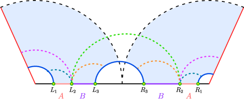
Figure 12: Diagrammatic representation of various phases of the EWCS (depicted as dashed curves) between subsystems $A$ and $B$ when the RT surface for $A\cup B$ is represented by the solid blue curves.

In this EE phase, we consider the subsystem $A$ to be close to boundary while B is far away. Hence, the EE for this phase corresponds to the sum of the lengths of the HM surface between points $L_{2}$ and $R_{3}$ and two island surfaces, shown as solid blue curves in fig. 12. The length of the HM surface and island surface is computed in eq. 15 and eq. 14 respectively. So by utilizing these equations, the EE for this phase may be written as

$$S_{2}=\frac{1}{4G_{N}}\log\left[\frac{u_{h}}{u_{L_{3}}u_{R_{3}}}\left(\Delta_{L_{3}}+\Delta_{R_{3}}+2\sqrt{\Delta_{L_{3}}\Delta_{R_{3}}}\cosh\frac{t}{u_{h}}\right)\right]+\frac{1}{2G_{N}}(2\rho_{\epsilon}-\rho_{B}).$$ (89)

As illustrated in fig. 12, there are four different phases of the reflected entropy or the bulk EWCS. In the following subsections, we explain the computation of the reflected entropy and bulk EWCS.

Phase-I

The reflected entropy or the bulk EWCS in this phase is similar to the first case of the section 4.1, shown as dashed green curve in fig. 12. Therefore, the bulk EWCS is given by eq. 77.

Phase-II

Reflected entropy:

In this reflected entropy phase, we assume that the subsystem $A$ is large enough, hence the six points twist correlator in numerator of eq. 71 may be factorized into a two-point and four one-point twist correlators in the BCFT₂ as follows

$$\langle\sigma_{g_{A}}(u_{L_{1}})\sigma_{g_{B}g_{A}^{-1}}(u_{L_{2}})\sigma_{g_{B}^{-1}}(u_{L_{3}})\sigma_{g_{B}}(u_{R_{3}})\sigma_{g_{A}g_{B}^{-1}}(u_{R_{2}})\sigma_{g_{A}^{-1}}(u_{R_{1}})\rangle_{\mathrm{BCFT}^{\bigotimes mn}}$$

$$=\langle\sigma_{g_{A}}(u_{L_{1}})\rangle_{\mathrm{BCFT}^{\bigotimes mn}}\langle\sigma_{g_{A}^{-1}}(u_{R_{1}})\rangle_{\mathrm{BCFT}^{\bigotimes mn}}\langle\sigma_{g_{B}^{-1}}(u_{L_{3}})\sigma_{g_{B}}(u_{R_{3}})\rangle_{\mathrm{CFT}^{\bigotimes mn}}$$

$$~{}~{}~{}~{}~{}~{}~{}~{}~{}~{}~{}~{}\times\langle\sigma_{g_{B}g_{A}^{-1}}(u_{L_{2}})\rangle_{\mathrm{BCFT}^{\bigotimes mn}}\langle\sigma_{g_{A}g_{B}^{-1}}(u_{R_{2}})\rangle_{\mathrm{BCFT}^{\bigotimes mn}},$$ (90)

where as the subsystem $A$ is close to the boundary, the BOE channel is favoured for the twist field correlator corresponding to the end points of $A$ while for the twist field correlator corresponding to the points ${L_{3}}$ and ${R_{3}}$ the OPE channel is favoured. The twist field correlator in the denominator of eq. 71 is also factorized similarly. Now by using eq. 71 the reflected entropy for this phase may be written as

$$S_{R}(A:B)=\lim_{{m,n}\to 1}\frac{1}{1-n}\log\langle\sigma_{g_{B}g_{A}^{-1}}(u_{L_{2}})\rangle_{\mathrm{BCFT}^{\bigotimes mn}}\langle\sigma_{g_{A}g_{B}^{-1}}(u_{R_{2}})\rangle_{\mathrm{BCFT}^{\bigotimes mn}}.$$ (91)

By utilizing eq. 7 and the expression of the one point function for the BCFT₂ on a black hole background Geng:2022dua , we may obtain the reflected entropy between the two adjacent subsystems as

$$S_{R}(A:B)=4\log g_{B}+\frac{2c}{3}\log\left(\frac{2}{\epsilon}\right).$$ (92)

EWCS:

The corresponding bulk EWCS is proportional to the sum of the lengths of two island surfaces, one beginning at point $L_{2}$ and ending at the EOW brane and the other starting at point $R_{2}$ and ending at the nearby EOW brane in the right TFD copy. These surfaces are depicted as dashed magenta curves in fig. 12. Now by utilizing the length of the island surface given in eq. 14, we may obtain the corresponding EWCS as

$$E_{W}(A:B)=\frac{1}{2G_{N}}(\rho_{\epsilon}-\rho_{B}).$$ (93)

Note that the reflected entropy computed in eq. 92 matches exactly with twice of the EWCS upon using eq. 16 and Brown-Henneaux relation.

Phase-III

Reflected entropy:

For this phase we consider that the subsystem $A$ is smaller than $B$, hence the six-point twist correlator in the numerator of eq. 71 may be factorized into three two-point twist correlators as follows

$$\langle\sigma_{g_{A}}(u_{L_{1}})\sigma_{g_{B}g_{A}^{-1}}(u_{L_{2}})\sigma_{g_{B}^{-1}}(u_{L_{3}})\sigma_{g_{B}}(u_{R_{3}})\sigma_{g_{A}g_{B}^{-1}}(u_{R_{2}})\sigma_{g_{A}^{-1}}(u_{R_{1}})\rangle_{\mathrm{BCFT}^{\bigotimes mn}}$$

$$=\langle\sigma_{g_{A}}(u_{L_{1}})\sigma_{g_{B}g_{A}^{-1}}(u_{L_{2}})\rangle_{\mathrm{BCFT}^{\bigotimes mn}}\langle\sigma_{g_{A}g_{B}^{-1}}(u_{R_{2}})\sigma_{g_{A}^{-1}}(u_{R_{1}})\rangle_{\mathrm{BCFT}^{\bigotimes mn}}\langle\sigma_{g_{B}^{-1}}(u_{L_{3}})\sigma_{g_{B}}(u_{R_{3}})\rangle_{\mathrm{BCFT}^{\bigotimes mn}}.$$ (94)

The last twist field correlator of the above equation cancels with a similar correlator originating from the factorization of the denominator in eq. 71. The remaining twist field correlators may be computed by transforming these to the twist field correlators defined on the conformally flat cylindrical background where the doubling trick is implemented Cardy:2004hm . The expression for the reflected entropy for this phase may then be written as follows

$$S_{R}(A:B)= \lim_{{m,n}\to 1}\frac{1}{1-n}\log\frac{\langle\sigma_{g_{A}}(u_{\star}({L_{1}}))\sigma_{g^{-1}_{A}}(-u_{\star}({L_{1}}))\sigma_{g_{B}g_{A}^{-1}}(u_{\star}({L_{2}}))\rangle_{\mathrm{CFT}^{\bigotimes mn}}}{\langle\sigma_{g_{m}}(u_{\star}({L_{1}}))\sigma_{g^{-1}_{m}}(-u_{\star}({L_{1}}))\rangle^{n}_{\mathrm{CFT}^{\bigotimes m}}}$$

$$+\lim_{{m,n}\to 1}\frac{1}{1-n}\log\frac{\langle\sigma_{g_{A}g_{B}^{-1}}(u_{\star}({R_{2}}))\sigma_{g_{A}^{-1}}(u_{\star}({R_{1}}))\sigma_{g_{A}}(-u_{\star}({R_{1}}))\rangle_{\mathrm{CFT}^{\bigotimes mn}}}{\langle\sigma_{g_{m}^{-1}}(u_{\star}({R_{1}}))\sigma_{g_{m}}(-u_{\star}({R_{1}}))\rangle^{n}_{\mathrm{CFT}^{\bigotimes m}}}.$$ (95)

Now by utilizing eq. 7 and the form of the flat plane three point twist correlator in section 4, the reflected entropy between two adjacent subsystems may be obtained as

$$S_{R}(A:B)= \frac{c}{3}\log\left[\frac{4u_{h}(\sqrt{\Delta_{L_{1}}}-\sqrt{\Delta_{L_{2}}})(-u_{h}+\Delta_{L_{1}}\Delta_{L_{2}})}{u_{L_{1}}u_{L_{2}}\epsilon}\right]$$

$$+\frac{c}{3}\log\left[\frac{4(\sqrt{\Delta_{R_{1}}}-\sqrt{\Delta_{R_{2}}})(-u_{h}+\Delta_{R_{1}}\Delta_{R_{2}})}{u_{R_{1}}u_{R_{2}}\epsilon}\right].$$ (96)

EWCS:

The bulk EWCS for this phase is proportional to the sum of the length of two geodesics one of which connects the point $L_{2}$ to an arbitrary point $(u_{L_{1}},\rho_{E},t)$ on the left island surface and second connects the point $R_{2}$ to an arbitrary point $(u_{R_{1}},\rho_{F},\tilde{t})$ on the right island surface. These geodesics are shown as dark green dashed curves in fig. 12. Now by using the embedding coordinates of points $L_{2}$ and $(u_{L_{1}},\rho_{E},t)$ in section 2.2.2, the length of the first geodesic may be written as

$$L=\log\left[\left(\frac{2u_{h}(\sqrt{\Delta_{L_{1}}}-\sqrt{\Delta_{L_{2}}})^{2}+u_{L_{1}}u_{L_{2}}}{u_{L_{1}}u_{L_{2}}}\right)\cosh\rho_{E}-\sinh\rho_{E}\right]+\rho_{\epsilon}.$$ (97)

The EWCS is obtained by extremizing the above expression with respect to $\rho_{E}$. The extremum value of $\rho_{E}$ is then given as

$$\rho_{E}=\frac{1}{2}\log\left(\frac{2u_{h}(\sqrt{\Delta_{L_{1}}}-\sqrt{\Delta_{L_{2}}})^{2}+u_{L_{1}}u_{L_{2}}}{u_{h}(\sqrt{\Delta_{L_{1}}}-\sqrt{\Delta_{L_{2}}})^{2}}\right).$$ (98)

Substituting this in eq. 97 and adding contribution from the right TFD copy, we may obtain the corresponding EWCS as

$$\small E_{W}(A:B)= \frac{1}{4G_{N}}\log\left[\frac{2e^{\rho_{\epsilon}}u_{h}(\sqrt{\Delta_{L_{1}}}-\sqrt{\Delta_{L_{2}}})(-u_{h}+\Delta_{L_{1}}\Delta_{L_{2}})}{u_{L_{1}}u_{L_{2}}}\right]$$

$$+\frac{1}{4G_{N}}\log\left[\frac{2e^{\rho_{\epsilon}}(\sqrt{\Delta_{R_{1}}}-\sqrt{\Delta_{R_{2}}})(-u_{h}+\Delta_{R_{1}}\Delta_{R_{2}})}{u_{R_{1}}u_{R_{2}}}\right].$$ (99)

Here also the above expression of the EWCS is matches exactly with half of the reflected entropy obtained in section 4 by utilizing eq. 16 and Brown-Henneaux relation.

Phase-IV

The reflected entropy or the bulk EWCS in this phase is similar to the first case of the section 4.1, shown as dashed orange curves in fig. 12. Therefore, the bulk EWCS is given by section 4.

4.3 Entanglement entropy phase 3

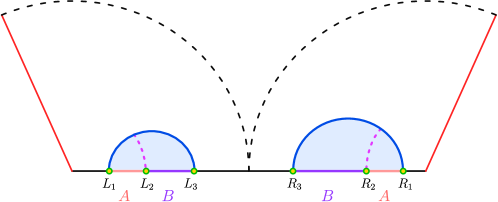
Figure 13: Schematic diagram of the EWCS (represented by dashed curves) between subsystems $A$ and $B$ when the RT surface for $AcupB$ is as depicted by the solid blue curves.

For this EE phase we assume that both the subsystems are very small and close to each other away from the boundary. Hence, the EE for this phase is proportional to the length of two dome-type RT surfaces, shown as solid blue curves in fig. 13. Now by utilizing the embedding coordinates of points $L_{1}$ and $L_{3}$ in section 2.2.2, the geodesic length of the dome-type RT surface may be written as

$$L=\log\left(\frac{u_{h}}{u_{L_{1}}u_{L_{3}}}(\sqrt{\Delta_{L_{1}}}-\sqrt{\Delta_{L_{3}}})^{2}\right)+2\rho_{\epsilon}.$$ (100)

Adding the contribution from the right TFD copy, the EE for this phase may be obtained as

$$S_{3}=\frac{1}{4G_{N}}\log\left(\frac{e^{2\rho_{\epsilon}}u_{h}}{u_{L_{1}}u_{L_{3}}}(\sqrt{\Delta_{L_{1}}}-\sqrt{\Delta_{L_{3}}})^{2}\right)+\frac{1}{4G_{N}}\log\left(\frac{e^{2\rho_{\epsilon}}u_{h}}{u_{R_{1}}u_{R_{3}}}(\sqrt{\Delta_{R_{1}}}-\sqrt{\Delta_{R_{3}}})^{2}\right).$$ (101)

For this EE phase we observe only one phase for the reflected entropy or the bulk EWCS, shown as dashed magenta curves in fig. 13. Here also the subsystems are away from the boundary, hence the OPE channel for the BCFT₂ correlator is favoured.

Reflected entropy:

For the reflected entropy computation in this phase, the six-point twist correlator in the numerator of eq. 71 may be factorized into two three-point twist correlators as

$$\langle\sigma_{g_{A}}(u_{L_{1}})\sigma_{g_{B}g_{A}^{-1}}(u_{L_{2}})\sigma_{g_{B}^{-1}}(u_{L_{3}})\sigma_{g_{B}}(u_{R_{3}})\sigma_{g_{A}g_{B}^{-1}}(u_{R_{2}})\sigma_{g_{A}^{-1}}(u_{R_{1}})\rangle_{\mathrm{CFT}^{\bigotimes mn}}$$

$$=\langle\sigma_{g_{A}}(u_{L_{1}})\sigma_{g_{B}g_{A}^{-1}}(u_{L_{2}})\sigma_{g^{-1}_{B}}(u_{L_{3}})\rangle_{\mathrm{CFT}^{\bigotimes mn}}\langle\sigma_{g^{-1}_{A}}(u_{R_{1}})\sigma_{g_{A}g_{B}^{-1}}(u_{R_{2}})\sigma_{g_{B}}(u_{R_{3}})\rangle_{\mathrm{CFT}^{\bigotimes mn}}.$$ (102)

The denominator of eq. 71 factorizes into two two-point twist correlators in the CFT₂. Hence the reflected entropy in this phase may be expressed as

$$S_{R}(A:B)= \lim_{{m,n}\to 1}\frac{1}{1-n}\log\frac{\langle\sigma_{g_{A}}(u_{L_{1}})\sigma_{g_{B}g_{A}^{-1}}(u_{L_{2}})\sigma_{g^{-1}_{B}}(u_{L_{3}})\rangle_{\mathrm{CFT}^{\bigotimes mn}}}{\langle\sigma_{g_{m}}(u_{L_{1}})\sigma_{g^{-1}_{m}}(u_{L_{3}})\rangle^{n}_{\mathrm{CFT}^{\bigotimes m}}}$$

$$+\lim_{{m,n}\to 1}\frac{1}{1-n}\log\frac{\langle\sigma_{g^{-1}_{A}}(u_{R_{1}})\sigma_{g_{A}g_{B}^{-1}}(u_{R_{2}})\sigma_{g_{B}}(u_{R_{3}})\rangle_{\mathrm{CFT}^{\bigotimes mn}}}{\langle\sigma_{g_{m}^{-1}}(u_{R_{1}})\sigma_{g_{m}}(u_{R_{3}})\rangle^{n}_{\mathrm{CFT}^{\bigotimes m}}}.$$ (103)

Now by utilizing eq. 7 and the form of three point twist correlator in the previous expression, the reflected entropy for this phase may be obtained as

$$S_{R}(A:B)= \frac{c}{3}\log\left[\frac{4u_{h}(\sqrt{\Delta_{L_{1}}}-\sqrt{\Delta_{L_{2}}})(\sqrt{\Delta_{L_{2}}}-\sqrt{\Delta_{L_{3}}})}{\epsilon\,u_{L_{2}}(\sqrt{\Delta_{L_{1}}}-\sqrt{\Delta_{L_{3}}})}\right]$$

$$+\frac{c}{3}\log\left[\frac{4(\sqrt{\Delta_{R_{1}}}-\sqrt{\Delta_{R_{2}}})(\sqrt{\Delta_{R_{2}}}-\sqrt{\Delta_{R_{3}}})}{\epsilon\,u_{R_{2}}(\sqrt{\Delta_{R_{1}}}-\sqrt{\Delta_{R_{3}}})}\right].$$ (104)

EWCS:

The bulk EWCS for this phase corresponds to the sum of the length of two geodesic, depicted as dashed magenta curves in fig. 13. Now, using the embedding coordinates of the points $L_{1}$, $L_{2}$ and $L_{3}$ in eq. 22 and adding contribution from the right TFD copy, the bulk EWCS may be obtained as

$$E_{W}(A:B)= \frac{1}{4G_{N}}\log\left[\frac{2e^{\rho_{\epsilon}}u_{h}(\sqrt{\Delta_{L_{1}}}-\sqrt{\Delta_{L_{2}}})(\sqrt{\Delta_{L_{2}}}-\sqrt{\Delta_{L_{3}}})}{u_{L_{2}}(\sqrt{\Delta_{L_{1}}}-\sqrt{\Delta_{L_{3}}})}\right]$$

$$+\frac{1}{4G_{N}}\log\left[\frac{2e^{\rho_{\epsilon}}(\sqrt{\Delta_{R_{1}}}-\sqrt{\Delta_{R_{2}}})(\sqrt{\Delta_{R_{2}}}-\sqrt{\Delta_{R_{3}}})}{u_{R_{2}}(\sqrt{\Delta_{R_{1}}}-\sqrt{\Delta_{R_{3}}})}\right].$$ (105)

Note that upon utilizing eq. 16 and Brown-Henneaux relation, the above expression of the bulk EWCS matches exactly with the half of the reflected entropy computed in section 4.3.

4.4 Entanglement entropy phase 4

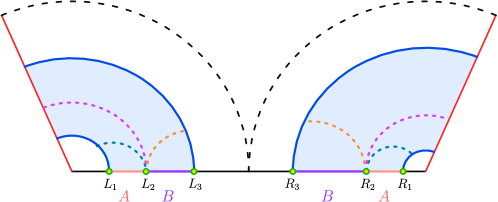
Figure 14: Schematic depicting the different phases of the EWCS (represented by various colored dashed curves) between subsystems $A$ and $B$ when the RT surface for $A\cup B$ is shown by the solid blue curves.

In this EE phase, we consider that both the subsystems $A$ and $B$ are very close to the boundary. So, the EE is proportional to the sum of the lengths of four island surfaces, shown as solid blue curves in fig. 14. Now by using eq. 14, the EE in this phase may be obtained as

$$S_{4}=\frac{1}{G_{N}}(\rho_{\epsilon}-\rho_{B}).$$ (106)

For this EE phase, there are three possible phases of the reflected entropy or the bulk EWCS, shown as dashed curves in fig. 14. In the following subsections, we describe the computation of the reflected entropy and the bulk EWCS.

Phase-I

The reflected entropy or the bulk EWCS in this phase is similar to the second case of the section 4.2, shown as dashed orange curves in fig. 14. Therefore, the bulk EWCS is given by eq. 93.

Phase-II

Reflected entropy:

In this phase, we assume subsystem $B$ is smaller than $A$. Therefore, the six-point twist field correlator in the numerator of eq. 71 may be factorized into two one-point twist field correlator and two two-point twist field correlator in BCFT₂ as

$$\langle\sigma_{g_{A}}(u_{L_{1}})\sigma_{g_{B}g_{A}^{-1}}(u_{L_{2}})\sigma_{g_{B}^{-1}}(u_{L_{3}})\sigma_{g_{B}}(u_{R_{3}})\sigma_{g_{A}g_{B}^{-1}}(u_{R_{2}})\sigma_{g_{A}^{-1}}(u_{R_{1}})\rangle_{\mathrm{BCFT}^{\bigotimes mn}}$$

$$=\langle\sigma_{g_{A}}(u_{L_{1}})\rangle_{\mathrm{BCFT}^{\bigotimes mn}}\langle\sigma_{g_{B}g_{A}^{-1}}(u_{L_{2}})\sigma_{g_{B}^{-1}}(u_{L_{3}})\rangle_{\mathrm{BCFT}^{\bigotimes mn}}$$

$$\quad\quad\quad\times\langle\sigma_{g_{A}^{-1}}(u_{R_{1}})\rangle_{\mathrm{BCFT}^{\bigotimes mn}}\langle\sigma_{g_{A}g_{B}^{-1}}(u_{R_{2}})\sigma_{g_{B}}(u_{R_{3}})\rangle_{\mathrm{BCFT}^{\bigotimes mn}}.$$ (107)

The two one-point twist field correlators of the above equation cancels with the denominator of eq. 71. To compute the remaining two two-point twist field correlator it is necessary to transform these to the twist field correlators defined on the conformally flat cylindrical background. Now using the doubling trick Cardy:2004hm and similar factorization in the denominator of eq. 71, the final expression for the reflected entropy in this case may be written as Li:2021dmf

$$S_{R}(A:B)= \lim_{{m,n}\to 1}\frac{1}{1-n}\log\frac{\langle\sigma_{g_{B}g_{A}^{-1}}(u_{\star}({L_{2}}))\sigma_{g_{B}^{-1}}(u_{\star}({L_{3}}))\sigma_{g_{B}}(-u_{\star}({L_{3}}))\rangle_{\mathrm{CFT}^{\bigotimes mn}}}{\langle\sigma_{g_{m}^{-1}}(u_{\star}({L_{3}}))\sigma_{g_{m}}(-u_{\star}({L_{3}}))\rangle^{n}_{\mathrm{CFT}^{\bigotimes m}}}$$

$$+\lim_{{m,n}\to 1}\frac{1}{1-n}\log\frac{\langle\sigma_{g_{A}g_{B}^{-1}}(u_{\star}({R_{2}}))\sigma_{g_{B}^{-1}}(u_{\star}({R_{3}}))\sigma_{g_{B}}(-u_{\star}({R_{3}}))\rangle_{\mathrm{CFT}^{\bigotimes mn}}}{\langle\sigma_{g{}_{m}}(u_{\star}({R_{3}}))\sigma_{g_{m}^{-1}}(-u_{\star}({R_{3}}))\rangle^{n}_{\mathrm{CFT}^{\bigotimes m}}}.$$ (108)

Utilizing eq. 7 and form of three-point function, the final expression for the reflected entropy may be obtained as

$$S_{R}(A:B)= \frac{c}{3}\log\left[\frac{4u_{h}(\sqrt{\Delta_{L_{2}}}-\sqrt{\Delta_{L_{3}}})(-u_{h}+\Delta_{L_{2}}\Delta_{L_{3}})}{\epsilon\,u_{L_{2}}u_{L_{3}}}\right]$$

$$+\frac{c}{3}\log\left[\frac{4(\sqrt{\Delta_{R_{2}}}-\sqrt{\Delta_{R_{3}}})(-u_{h}+\Delta_{R_{2}}\Delta_{R_{3}})}{\epsilon\,u_{R_{2}}u_{R_{3}}}\right].$$ (109)

EWCS:

The bulk EWCS for this phase is given by the sum of the lengths of two geodesics in which one connects the point $L_{2}$ to an arbitrary point $(u_{L_{3}},\rho_{Y},t)$ on the island surface and another joins the point $R_{2}$ to an arbitrary point $(u_{R_{3}},\rho_{Z},\tilde{t})$ on the island surface for the right TFD copy. These geodesics are shown as orange dashed curves in fig. 14. Now by utilizing the embedding coordinates of points $L_{2}$ and $(u_{L_{3}},\rho_{Y},t)$ in section 2.2.2, the length of the first geodesic may be written as

$$L=\log\left[\left(\frac{2u_{h}(\sqrt{\Delta_{L_{2}}}-\sqrt{\Delta_{L_{3}}})^{2}+u_{L_{2}}u_{L_{3}}}{u_{L_{2}}u_{L_{3}}}\right)\cosh\rho_{Y}-\sinh\rho_{Y}\right]+\rho_{\epsilon}.$$ (110)

To obtain the EWCS, we need to extremize the above expression with respect to $\rho_{Y}$. The extremum value of $\rho_{Y}$ is given as

$$\rho_{Y}=\frac{1}{2}\log\left(\frac{2u_{h}(\sqrt{\Delta_{L_{2}}}-\sqrt{\Delta_{L_{3}}})^{2}+u_{L_{2}}u_{L_{3}}}{u_{h}(\sqrt{\Delta_{L_{2}}}-\sqrt{\Delta_{L_{3}}})^{2}}\right),$$ (111)

Substituting the above in eq. 110 and adding the contribution for the right TFD copy, the corresponding bulk EWCS may be obtained as

$$E_{W}(A:B)= \frac{1}{4G_{N}}\log\left[\frac{2e^{\rho_{\epsilon}}u_{h}(\sqrt{\Delta_{L_{2}}}-\sqrt{\Delta_{L_{3}}})(-u_{h}+\Delta_{L_{2}}\Delta_{L_{3}})}{u_{L_{2}}u_{L_{3}}}\right]$$

$$+\frac{1}{4G_{N}}\log\left[\frac{2e^{\rho_{\epsilon}}(\sqrt{\Delta_{R_{2}}}-\sqrt{\Delta_{R_{3}}})(-u_{h}+\Delta_{R_{2}}\Delta_{R_{3}})}{u_{R_{2}}u_{R_{3}}}\right].$$ (112)

Here also the reflected entropy obtained in section 4 matches exactly with twice of the EWCS upon utilizing eq. 16 and Brown-Henneaux relation.

Phase-III

The reflected entropy or the bulk EWCS in this phase is similar to the third case of the section 4.2, shown as dark green dashed curves in fig. 14. Therefore, the bulk EWCS is given by section 4.

4.5 Page curve

In this subsection we illustrate the analogue of the Page curves for the reflected entropy for two adjacent subsystems in a BCFT₂ on an AdS₂ black hole background.

4.5.1 Case-I

The EE phase transition between phase-2 and phase-4 may be obtained by utilizing a small brane angle (corresponding to a small boundary entropy) and taking subsystem $B$ away from the boundary, as shown in fig. 15(a). The Page time $T^{\text{adj}}_{{2\rightarrow 4}}$ for this transition is given as

$$T^{\text{adj}}_{{2\rightarrow 4}}=u_{h}\cosh^{-1}\left(\frac{u^{2}_{h}-u_{h}\left(e^{2\rho_{B}}+1\right)(\Delta_{L_{3}}+\Delta_{R_{3}})+\Delta_{L_{3}}\Delta_{R_{3}}}{2u_{h}e^{2\rho_{B}}\sqrt{\Delta_{L_{3}}\Delta_{R_{3}}}}\right).$$ (113)

We now investigate the Page curve for the reflected entropy in these EE phases, depicted in fig. 15(b). Initially in the EE phase-2 the reflected entropy increases with time as the bulk EWCS is the HM surface, then remains constant until Page time as the growth rate of the bulk EWCS which lands on the HM surface is almost similar to that of the HM surface. After the Page time, in the EE phase-4 it saturates to another constant value. From the Page curve of the reflected entropy we observe that initially the Markov gap is zero as the bulk EWCS phase has no non-trivial boundaries but after some time for the same bulk EWCS phase this gap becomes non-zero as the mutual information undergoes a phase transition. After that this gap increases to a value greater than $\frac{2c}{3}\log{2}$ as the bulk EWCS phase has two non-trivial boundaries. Furthermore, after the Page time, the Markov gap saturates to the lower bound mentioned in eq. 23.

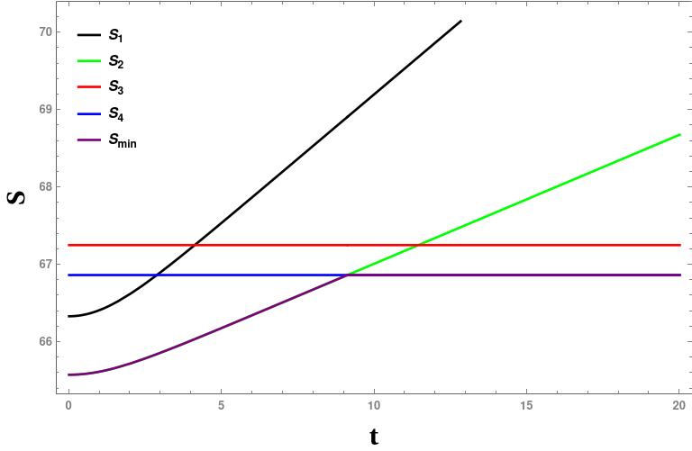
((a))

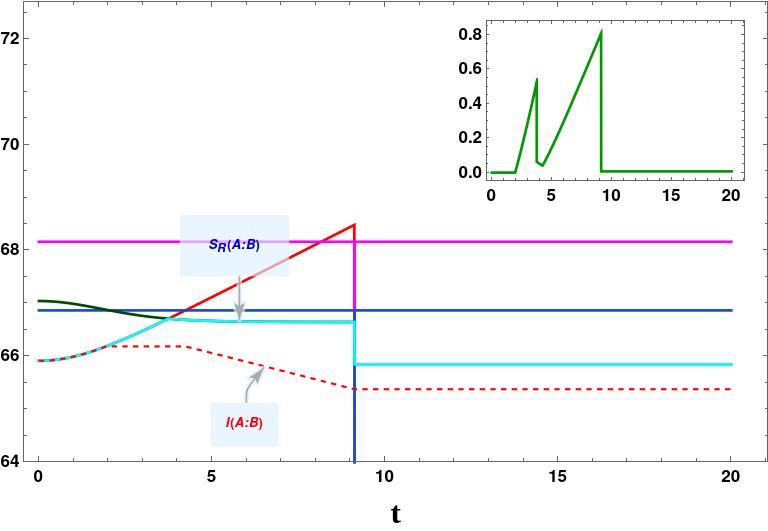
((b))

Figure 15: (a) Page curve of the EE for subsystems $A\cup B$. Here purple colour shows the minimum EE among all the phases. (b) Page curve of the reflected entropy between subsystems $A$ and $B$. Here cyan colour represents minimum $S_{R}$ and red dashed line is mutual information (All graphs are in units of $c$). The inset plot shows the deviation from saturation of the Markov gap eq. 23. The Page curves for the EE and $S_{R}$ is obtained with $u_{h}=1,\Delta_{L_{1}}=0.9,\Delta_{L_{2}}=3\times 10^{-2},\Delta_{L_{3}}=2\times 10^{-4},\Delta_{R_{1}}=0.8,\Delta_{R_{2}}=2\times 10^{-2},\Delta_{R_{3}}=2\times 10^{-4},\rho_{B}=-0.3,\rho_{\epsilon}=100$.

4.5.2 Case-II

The EE transition between phase-2 and phase-3 may be obtained by taking a small brane angle and subsystem $B$ is relatively away form the boundary than the previous case, as depicted in fig. 16(a). The Page time for this transition is given as

$$T^{\text{adj}}_{{2\rightarrow 3}}=u_{h}\cosh^{-1}\left(\frac{u_{h}e^{2\rho_{B}}\left(\sqrt{\Delta_{L_{1}}}-\sqrt{\Delta_{L_{3}}}\right)^{2}\left(\sqrt{\Delta_{R_{1}}}-\sqrt{\Delta_{R_{3}}}\right)^{2}}{2u_{L_{1}}u_{R_{1}}\sqrt{\Delta_{L_{3}}\Delta_{R_{3}}}}-\frac{(\Delta_{L_{3}}+\Delta_{R_{3}})}{2\sqrt{\Delta_{L_{3}}\Delta_{R_{3}}}}\right).$$ (114)

The Page curve of the reflected entropy for these EE phases is shown in fig. 16(b). The reflected entropy in phase-2 first increases as the bulk EWCS is the HM surface, then remains constant until Page time as the bulk EWCS lands on the EOW brane. Finally after the Page time, it saturates to another constant value in phase-3. Initially the Markov gap should be zero as the bulk EWCS has no non-trivial boundary however it is observed to be non-zero which contradicts the geometric interpretation of the Markov gap described in eq. 23 suggesting a critical re-examination of this issue in the context of the AdS/BCFT scenario. Subsequently with time this gap increases to a value greater than $\frac{2c}{3}\log{2}$ as two non-trivial boundaries of the bulk EWCS appear in the corresponding phase. Furthermore after the Page time, this gap saturates to the lower bound mentioned in eq. 23 which was expected as the computation of the reflected entropy reduces to the usual CFT which involves the contribution from the OPE channel of the corresponding BCFT correlators.

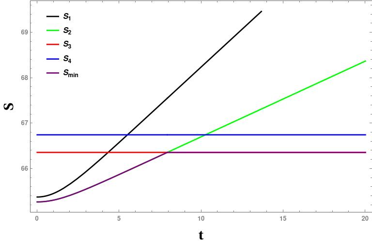
((a))

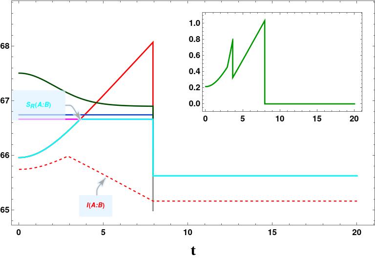
((b))

Figure 16: (a) Page curve of the EE for subsystems $A\cup B$. Here purple colour shows the minimum EE among all the phases. (b) Page curve of the reflected entropy between subsystems $A$ and $B$. Here cyan colour represents minimum $S_{R}$ and red dashed line is mutual information (All graphs are in units of $c$). The inset plot shows the deviation from saturation of the Markov gap eq. 23. The Page curves for the EE and $S_{R}$ is obtained with $u_{h}=1,\Delta_{L_{1}}=0.4,\Delta_{L_{2}}=5.8\times 10^{-2},\Delta_{L_{3}}=4\times 10^{-5},\Delta_{R_{1}}=0.2,\Delta_{R_{2}}=.915\times 10^{-2},\Delta_{R_{3}}=5\times 10^{-5},\rho_{B}=-0.12,\rho_{\epsilon}=100$.

4.5.3 Case-III

The EE transition between phase-1 and phase-2 at time $T^{\text{adj}}_{{1\rightarrow 2}}$ which is same as $T^{\text{disj}}_{{1\rightarrow 2}}$, and phase-2 and phase-3 at time $T^{\text{adj}}_{{2\rightarrow 3}}$ may be obtained by taking a relatively large brane angle and subsystem $B$ is far away from the boundary than the previous two cases as depicted in fig. 17(a). The Page times for these EE transition $T^{\text{adj}}_{{1\rightarrow 2}}$ and $T^{\text{adj}}_{{2\rightarrow 3}}$ are given in eq. 68 and eq. 114 respectively. In the EE phase-1, the reflected entropy increases initially as the bulk EWCS is the HM surface and then slowly decreases until Page time $T^{\text{adj}}_{{1\rightarrow 2}}$ as the growth rate of the bulk EWCS which lands on the HM surface is lower than that of the HM surface. After the Page time in the EE phase-2, it again increases as the bulk EWCS is again the HM surface and then remains constant until Page time $T^{\text{adj}}_{{2\rightarrow 3}}$. Finally in the EE phase-3, it saturates to a constant value. The reflected entropy Page curve is shown in fig. 17(b). The Page curve of the reflected entropy indicates that in the EE phase-1, initially the Markov gap is zero as there are no non-trivial boundaries of the bulk EWCS, however as earlier this gap becomes non zero with time due to a phase transition in the mutual information. Subsequently as earlier this gap increases to a value greater than $\frac{2c}{3}\log{2}$ as two non-trivial boundaries of the bulk EWCS appear in this phase. Furthermore after the Page time in the EE phase-2, this gap is always greater than $\frac{2c}{3}\log{2}$. Finally, in the EE phase-3, this gap saturates to the lower bound given in eq. 23 which was also expected (c.f. section 4.5.2).

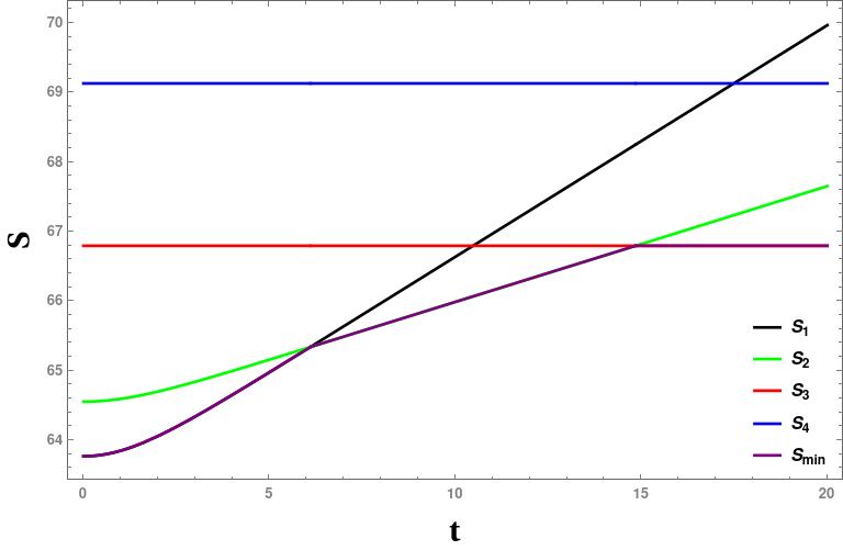
((a))

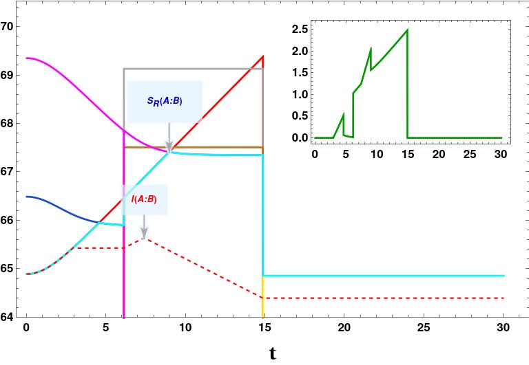
((b))

Figure 17: (a) Page curve of the EE for subsystems $A\cup B$. Here purple colour shows the minimum EE among all the phases. (b) Page curve of the reflected entropy between subsystems $A$ and $B$. Here cyan colour represents minimum $S_{R}$ and red dashed line is mutual information (All graphs are in units of $c$). The inset plot shows the deviation from saturation of the Markov gap eq. 23. The Page curves for the EE and $S_{R}$ is obtained with $u_{h}=1,\Delta_{L_{1}}=0.6,\Delta_{L_{2}}=15\times 10^{-4},\Delta_{L_{3}}=5\times 10^{-10},\Delta_{R_{1}}=0.592223,\Delta_{R_{2}}=9.9\times 10^{-4},\Delta_{R_{3}}=4.5\times 10^{-10},\rho_{B}=-3.7,\rho_{\epsilon}=100$.

4.5.4 Case-IV

The EE transition between the EE phase-1 and phase-3 may be obtained by using a small brane angle and taking the subsystem $B$ is close to the boundary than first two cases as shown in fig. 18(a). The Page time for this transition is given as

$$T^{\text{Adj.}}_{{1\rightarrow 3}}=\cosh^{-1}\left(\frac{\Delta_{L_{1}}+\Delta_{R_{1}}}{\sqrt{\Delta_{L_{1}}\Delta_{R_{1}}}}+\frac{\Delta_{L_{3}}+\Delta_{R_{3}}}{\sqrt{\Delta_{L_{3}}\Delta_{R_{3}}}}-A^{2}\right),$$ (115)

where

$$A^{2}= \left(\frac{\Delta_{L_{1}}}{\Delta_{R_{1}}}+\frac{\Delta_{R_{1}}}{\Delta_{L_{1}}}\right)+\left(\frac{\Delta_{L_{3}}}{\Delta_{R_{3}}}+\frac{\Delta_{R_{3}}}{\Delta_{L_{3}}}\right)-8\Delta_{L_{1}}\Delta_{L_{3}}\Delta_{R_{1}}\Delta_{R_{3}}\left(\frac{\Delta_{L_{1}}+\Delta_{L_{3}}}{\sqrt{\Delta_{L_{1}}\Delta_{L_{3}}}}+\frac{\Delta_{R_{1}}+\Delta_{R_{3}}}{\sqrt{\Delta_{R_{1}}\Delta_{R_{3}}}}\right)$$

$$+20+\frac{2\Delta_{L_{1}}(-\Delta_{L_{3}}+2\Delta_{R_{1}}+\Delta_{R_{3}})+2\Delta_{L_{3}}(\Delta_{R_{1}}+2\Delta_{R_{3}})-2\Delta_{R_{1}}\Delta_{R_{3}}}{\sqrt{\Delta_{L_{1}}\Delta_{L_{3}}\Delta_{R_{1}}\Delta_{R_{3}}}}.$$ (116)

From the Page curve of the reflected entropy, we observe that in the EE phase-1, the reflected entropy increases initially as the bulk EWCS is the HM surface and then slowly decreases until Page time as the growth rate of the bulk EWCS which lands on the HM surface is lower than that of the HM surface. After the Page time, in the EE phase-3, it saturates to a constant value. Here also initially the Markov gap should be zero as the bulk EWCS has no non-trivial boundaries however it is observed to be non zero which again suggests further critical analysis of the geometric interpretation. Subsequently till the Page time $T^{\text{adj}}_{{1\rightarrow 3}}$, it is always greater than $\frac{2c}{3}\log{2}$ as the bulk EWCS has two non-trivial boundaries. Furthermore after the Page time, it saturates to the lower bound given in eq. 23 which was also expected (c.f. section 4.5.2).

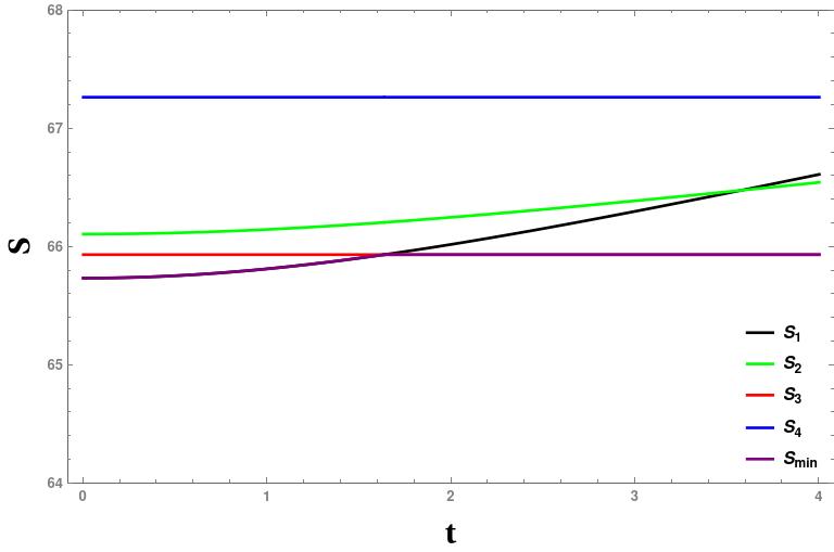
((a))

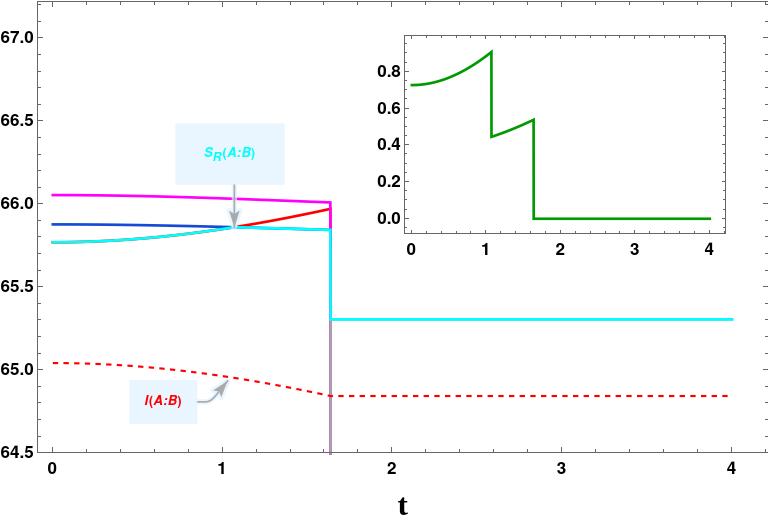
((b))

Figure 18: (a) Page curve of the EE for subsystems $A\cup B$. Here purple colour shows the minimum EE among all the phases. (b) Page curve of the reflected entropy between subsystems $A$ and $B$. Here cyan colour represents minimum $S_{R}$ and red dashed line is mutual information (All graphs are in units of $c$). The inset plot shows the deviation from saturation of the Markov gap eq. 23. The Page curves for the EE and $S_{R}$ is obtained with $u_{h}=1,\Delta_{L_{1}}=0.15,\Delta_{L_{2}}=1.8\times 10^{-2},\Delta_{L_{3}}=2\times 10^{-3},\Delta_{R_{1}}=0.1,\Delta_{R_{2}}=1.5\times 10^{-2},\Delta_{R_{3}}=1\times 10^{-3},\rho_{B}=-0.9,\rho_{\epsilon}=100$.

5 Summary and discussion

In this article, we have investigated the mixed state entanglement structure through the reflected entropy, in the KR braneworld model with the radiation bath located in a gravitational background. In particular, we considered an AdS₃ black string geometry truncated by a EOW brane for which the lower dimensional effective perspective consists of a gravitating radiation bath. In this connection, the dual BCFT₂ is defined on an eternal AdS₂ black hole background. We have obtained the reflected entropy for various bipartite mixed state configurations involving two disjoint and adjacent subsystems in the BCFT₂. Furthermore, we have elucidated the phase structure for the reflected entropy arising from various factorizations of the twist field correlators in the large central charge limit after identifying the EE phases. Subsequently, we have computed the corresponding EWCS in the dual bulk AdS₃ black string geometry for the bipartite mixed states under consideration. It is further demonstrated that our holographic computations match identically with the field theory replica technique results in the large central charge limit for all the phases.

Following the above, we have also obtained the Page curves for the EE and within each phase of the EE, we observed rich phase structure for the holographic reflected entropy depending on the boundary entropy, the location of the subsystems and their relative separation from the boundary. Furthermore, we have also compared the reflected entropy with the holographic mutual information in order to investigate the Markov gap. For all the phases of the reflected entropy, we have shown the deviation of the Markov gap from its saturation value. Interestingly, we observed that for the phases of the bulk EWCS involving the HM surface in the bulk geometry, the Markov gap is non-zero even when there are no non-trivial boundaries of the EWCS, which is not obvious from the standard geometric interpretation provided in Hayden:2021gno . As a result, it will be interesting to investigate this interpretation in the braneworld geometry.

From the Page curve of the reflected entropy we observed that there are sudden jumps or drops at the Page time whose origin may be attributed to the specific choice of the Rényi entanglement entropy saddle i.e., fully connected and fully disconnected replica wormhole saddles. These discontinuities may be smoothened out by considering all possible Rényi entanglement entropy saddles Penington:2019kki . However we may still miss some Rényi reflected entropy saddles. Thus to obtain a proper (continuous and smooth) Page curve for the reflected entropy as in Akers:2022max , one should include contributions from all Rényi reflected entropy saddles in each Rényi entanglement entropy saddle in the corresponding gravitational path integral which is computationally challenging and beyond the scope of the present work.

There are several future directions to explore. It will be interesting to investigate other mixed state entanglement and correlation measures such as entanglement negativity, entanglement of purification, balance partial entanglement in this braneworld model. One may also generalize our study to higher dimensions and to multipartite entanglement and correlations. This model may also be generalized for two boundary BCFT with black holes induced on the each of the two corresponding EOW branes. It would be interesting to investigate the interaction between these two black holes in this scenario. Another significant generalization of this braneworld model could be the study of mixed state entanglement for two CFTs defined on a black hole background communicating through a shared interface. We leave these interesting open issue for future consideration.

Appendix A Geodesics between two minimal surfaces

The EWCS for some configurations may be obtained by computing the geodesic distance between two geodesics. In the embedding coordinates, the length of the geodesics ending on the bulk points $X_{i}$ and $X_{j}$ is given by

$$\sigma(X_{i},X_{j}) =\cosh^{-1}\xi_{ij},~{}~{}~{}~{}~{}~{}~{}~{}~{}~{}\xi_{ij}=-X_{i}\cdot X_{j}.$$ (117)

A.1 Geodesic between a fixed boundary point and a bulk geodesic

A spacelike geodesic anchored on two boundary points $X_{1}$ and $X_{3}$ may be parametrized by an affine parameter $\lambda$ as follows

$$X_{13}^{A}(\lambda)=\frac{X^{A}_{1}e^{-\lambda}+X^{A}_{3}e^{\lambda}}{\sqrt{-2X_{1}\cdot X_{3}}}.$$ (118)

By utilizing eq. 117, the geodesic length between a fixed boundary point $X_{2}$ and a geodesic $X_{13}(\lambda)$ may be written as

$$\sigma(X_{13},X_{2})=\cosh^{-1}\left[\frac{\xi_{12}e^{-\lambda}+\xi_{23}e^{-\lambda}}{\sqrt{2\xi_{13}}}\right].$$ (119)

Now by extremizing this length over $\lambda$ and substituting back the extremum value in eq. 119 we may obtained the EWCS between a fixed boundary point and a bulk geodesic as

$$E_{W}=\frac{1}{4G_{N}}\cosh^{-1}\left(\sqrt{\frac{2\xi_{12}\xi_{23}}{\xi_{13}}}\right).$$ (120)

A.2 Geodesic between one bulk point and three boundary point

The spacelike geodesic $X_{14}(\lambda)$ anchored on two bulk points $X_{1}$ and $X_{4}$ is given as

$$X_{14}(\lambda)=e^{\lambda}\left(\frac{X_{4}}{\sqrt{2\xi_{14}}}-\frac{X_{1}}{(2\xi_{14})^{3/2}}\right)+e^{-\lambda}\left(\frac{X_{1}}{\sqrt{2\xi_{14}}}-\frac{X_{4}}{(2\xi_{14})^{3/2}}\right),$$ (121)

and a spacelike geodesic $X_{23}(\lambda_{p})$ anchored between two boundary points $X_{2}$ and $X_{3}$ is given as

$$X_{23}(\lambda_{p})=\frac{e^{-\lambda_{p}}X_{2}+e^{\lambda_{p}}X_{3}}{\sqrt{2\xi_{23}}}.$$ (122)

Now by utilizing the eq. 117, the length of the geodesic between $X_{14}(\lambda)$ and $X_{23}(\lambda_{p})$ may be written as

$$\sigma({X_{14},X_{23}})=\cosh^{-1}\left(-X_{14}\cdot X_{23}\right).$$ (123)

By extremizing this length over $\lambda$ and $\lambda_{p}$ and putting back their extremum value in eq. 123,the EWCS may be obtained as

$$E_{W}=\cosh^{-1}\left(\frac{2\xi_{14}\xi_{34}-\sqrt{\frac{(\xi_{12}-2\xi_{14}\xi_{24})(2\xi_{13}\xi_{14}-\xi_{34})(\xi_{13}-2\xi_{14}\xi_{34})}{2\xi_{12}\xi_{14}-\xi_{24}}}-\xi_{13}}{2\xi_{14}^{3/2}\sqrt{{\xi_{23}}}\sqrt{\frac{2\xi_{14}\xi_{34}-\xi_{13}}{2\xi_{12}\xi_{14}-\xi_{24}}}}\right).$$ (124)

References

- (1) S. W. Hawking, “Particle Creation by Black Holes,” Commun. Math. Phys. 43 (1975) 199–220. [Erratum: Commun.Math.Phys. 46, 206 (1976)].
- (2) S. W. Hawking, “Breakdown of Predictability in Gravitational Collapse,” Phys. Rev. D 14 (1976) 2460–2473.
- (3) G. Penington, “Entanglement Wedge Reconstruction and the Information Paradox,” JHEP 09 (2020) 002, arXiv:1905.08255 [hep-th].
- (4) A. Almheiri, N. Engelhardt, D. Marolf, and H. Maxfield, “The entropy of bulk quantum fields and the entanglement wedge of an evaporating black hole,” JHEP 12 (2019) 063, arXiv:1905.08762 [hep-th].
- (5) A. Almheiri, R. Mahajan, J. Maldacena, and Y. Zhao, “The Page curve of Hawking radiation from semiclassical geometry,” JHEP 03 (2020) 149, arXiv:1908.10996 [hep-th].
- (6) A. Almheiri, R. Mahajan, and J. Maldacena, “Islands outside the horizon,” arXiv:1910.11077 [hep-th].
- (7) G. Penington, S. H. Shenker, D. Stanford, and Z. Yang, “Replica wormholes and the black hole interior,” JHEP 03 (2022) 205, arXiv:1911.11977 [hep-th].
- (8) A. Almheiri, T. Hartman, J. Maldacena, E. Shaghoulian, and A. Tajdini, “The entropy of Hawking radiation,” Rev. Mod. Phys. 93 no. 3, (2021) 035002, arXiv:2006.06872 [hep-th].
- (9) S. Ryu and T. Takayanagi, “Holographic derivation of entanglement entropy from AdS/CFT,” Phys. Rev. Lett. 96 (2006) 181602, arXiv:hep-th/0603001.
- (10) S. Ryu and T. Takayanagi, “Aspects of Holographic Entanglement Entropy,” JHEP 08 (2006) 045, arXiv:hep-th/0605073.
- (11) V. E. Hubeny, M. Rangamani, and T. Takayanagi, “A Covariant holographic entanglement entropy proposal,” JHEP 07 (2007) 062, arXiv:0705.0016 [hep-th].
- (12) T. Faulkner, A. Lewkowycz, and J. Maldacena, “Quantum corrections to holographic entanglement entropy,” JHEP 11 (2013) 074, arXiv:1307.2892 [hep-th].
- (13) N. Engelhardt and A. C. Wall, “Quantum Extremal Surfaces: Holographic Entanglement Entropy beyond the Classical Regime,” JHEP 01 (2015) 073, arXiv:1408.3203 [hep-th].
- (14) D. N. Page, “Information in black hole radiation,” Phys. Rev. Lett. 71 (1993) 3743–3746, arXiv:hep-th/9306083.
- (15) D. N. Page, “Average entropy of a subsystem,” Phys. Rev. Lett. 71 (1993) 1291–1294, arXiv:gr-qc/9305007.
- (16) D. N. Page, “Time Dependence of Hawking Radiation Entropy,” JCAP 09 (2013) 028, arXiv:1301.4995 [hep-th].
- (17) A. Almheiri, T. Hartman, J. Maldacena, E. Shaghoulian, and A. Tajdini, “Replica Wormholes and the Entropy of Hawking Radiation,” JHEP 05 (2020) 013, arXiv:1911.12333 [hep-th].
- (18) X. Dong, X.-L. Qi, Z. Shangnan, and Z. Yang, “Effective entropy of quantum fields coupled with gravity,” JHEP 10 (2020) 052, arXiv:2007.02987 [hep-th].
- (19) K. Kawabata, T. Nishioka, Y. Okuyama, and K. Watanabe, “Replica wormholes and capacity of entanglement,” JHEP 10 (2021) 227, arXiv:2105.08396 [hep-th].
- (20) M. Rozali, J. Sully, M. Van Raamsdonk, C. Waddell, and D. Wakeham, “Information radiation in BCFT models of black holes,” JHEP 05 (2020) 004, arXiv:1910.12836 [hep-th].
- (21) H. Z. Chen, R. C. Myers, D. Neuenfeld, I. A. Reyes, and J. Sandor, “Quantum Extremal Islands Made Easy, Part I: Entanglement on the Brane,” JHEP 10 (2020) 166, arXiv:2006.04851 [hep-th].
- (22) H. Z. Chen, R. C. Myers, D. Neuenfeld, I. A. Reyes, and J. Sandor, “Quantum Extremal Islands Made Easy, Part II: Black Holes on the Brane,” JHEP 12 (2020) 025, arXiv:2010.00018 [hep-th].
- (23) F. Deng, J. Chu, and Y. Zhou, “Defect extremal surface as the holographic counterpart of Island formula,” JHEP 03 (2021) 008, arXiv:2012.07612 [hep-th].
- (24) K. Suzuki and T. Takayanagi, “BCFT and Islands in two dimensions,” JHEP 06 (2022) 095, arXiv:2202.08462 [hep-th].
- (25) G. Grimaldi, J. Hernandez, and R. C. Myers, “Quantum extremal islands made easy. Part IV. Massive black holes on the brane,” JHEP 03 (2022) 136, arXiv:2202.00679 [hep-th].
- (26) H. Geng and A. Karch, “Massive islands,” JHEP 09 (2020) 121, arXiv:2006.02438 [hep-th].
- (27) H. Geng, A. Karch, C. Perez-Pardavila, S. Raju, L. Randall, M. Riojas, and S. Shashi, “Information Transfer with a Gravitating Bath,” SciPost Phys. 10 no. 5, (2021) 103, arXiv:2012.04671 [hep-th].
- (28) H. Geng, S. Lüst, R. K. Mishra, and D. Wakeham, “Holographic BCFTs and Communicating Black Holes,” JHEP 08 (2021) 003, arXiv:2104.07039 [hep-th].
- (29) H. Geng, A. Karch, C. Perez-Pardavila, S. Raju, L. Randall, M. Riojas, and S. Shashi, “Entanglement phase structure of a holographic BCFT in a black hole background,” JHEP 05 (2022) 153, arXiv:2112.09132 [hep-th].
- (30) H. Geng, A. Karch, C. Perez-Pardavila, S. Raju, L. Randall, M. Riojas, and S. Shashi, “Inconsistency of islands in theories with long-range gravity,” JHEP 01 (2022) 182, arXiv:2107.03390 [hep-th].
- (31) T. Takayanagi, “Holographic Dual of BCFT,” Phys. Rev. Lett. 107 (2011) 101602, arXiv:1105.5165 [hep-th].
- (32) M. Fujita, T. Takayanagi, and E. Tonni, “Aspects of AdS/BCFT,” JHEP 11 (2011) 043, arXiv:1108.5152 [hep-th].
- (33) A. Karch and L. Randall, “Locally localized gravity,” JHEP 05 (2001) 008, arXiv:hep-th/0011156.
- (34) A. Karch and L. Randall, “Open and closed string interpretation of SUSY CFT’s on branes with boundaries,” JHEP 06 (2001) 063, arXiv:hep-th/0105132.
- (35) S. Raju, “Lessons from the information paradox,” Phys. Rept. 943 (2022) 1–80, arXiv:2012.05770 [hep-th].
- (36) H. Geng, L. Randall, and E. Swanson, “BCFT in a black hole background: an analytical holographic model,” JHEP 12 (2022) 056, arXiv:2209.02074 [hep-th].
- (37) G. Vidal and R. F. Werner, “Computable measure of entanglement,” Phys. Rev. A 65 (2002) 032314, arXiv:quant-ph/0102117.
- (38) M. B. Plenio, “Logarithmic Negativity: A Full Entanglement Monotone That is not Convex,” Phys. Rev. Lett. 95 no. 9, (2005) 090503, arXiv:quant-ph/0505071.
- (39) P. Calabrese, J. Cardy, and E. Tonni, “Entanglement negativity in quantum field theory,” Phys. Rev. Lett. 109 (2012) 130502, arXiv:1206.3092 [cond-mat.stat-mech].
- (40) P. Calabrese, J. Cardy, and E. Tonni, “Entanglement negativity in extended systems: A field theoretical approach,” J. Stat. Mech. 1302 (2013) P02008, arXiv:1210.5359 [cond-mat.stat-mech].
- (41) P. Calabrese, J. Cardy, and E. Tonni, “Finite temperature entanglement negativity in conformal field theory,” J. Phys. A 48 no. 1, (2015) 015006, arXiv:1408.3043 [cond-mat.stat-mech].
- (42) S. Dutta and T. Faulkner, “A canonical purification for the entanglement wedge cross-section,” JHEP 03 (2021) 178, arXiv:1905.00577 [hep-th].
- (43) H.-S. Jeong, K.-Y. Kim, and M. Nishida, “Reflected Entropy and Entanglement Wedge Cross Section with the First Order Correction,” JHEP 12 (2019) 170, arXiv:1909.02806 [hep-th].
- (44) B. M. Terhal, M. Horodecki, D. W. Leung, and D. P. DiVincenzo, “The entanglement of purification,” Journal of Mathematical Physics 43 no. 9, (2002) 4286–4298, https://doi.org/10.1063/1.1498001. https://doi.org/10.1063/1.1498001.
- (45) T. Takayanagi and K. Umemoto, “Entanglement of purification through holographic duality,” Nature Phys. 14 no. 6, (2018) 573–577, arXiv:1708.09393 [hep-th].
- (46) K. Tamaoka, “Entanglement Wedge Cross Section from the Dual Density Matrix,” Phys. Rev. Lett. 122 no. 14, (2019) 141601, arXiv:1809.09109 [hep-th].
- (47) Q. Wen, “Balanced Partial Entanglement and the Entanglement Wedge Cross Section,” JHEP 04 (2021) 301, arXiv:2103.00415 [hep-th].
- (48) T. Li, J. Chu, and Y. Zhou, “Reflected Entropy for an Evaporating Black Hole,” JHEP 11 (2020) 155, arXiv:2006.10846 [hep-th].
- (49) T. Li, M.-K. Yuan, and Y. Zhou, “Defect extremal surface for reflected entropy,” JHEP 01 (2022) 018, arXiv:2108.08544 [hep-th].
- (50) Y. Shao, M.-K. Yuan, and Y. Zhou, “Entanglement Negativity and Defect Extremal Surface,” arXiv:2206.05951 [hep-th].
- (51) J. Basak Kumar, D. Basu, V. Malvimat, H. Parihar, and G. Sengupta, “Reflected entropy and entanglement negativity for holographic moving mirrors,” JHEP 09 (2022) 089, arXiv:2204.06015 [hep-th].
- (52) D. Basu, H. Parihar, V. Raj, and G. Sengupta, “Defect extremal surfaces for entanglement negativity,” Phys. Rev. D 108 no. 10, (2023) 106005, arXiv:2205.07905 [hep-th].
- (53) M. Afrasiar, J. Kumar Basak, A. Chandra, and G. Sengupta, “Islands for entanglement negativity in communicating black holes,” Phys. Rev. D 108 no. 6, (2023) 066013, arXiv:2205.07903 [hep-th].
- (54) M. Afrasiar, J. K. Basak, A. Chandra, and G. Sengupta, “Reflected entropy for communicating black holes. Part I. Karch-Randall braneworlds,” JHEP 02 (2023) 203, arXiv:2211.13246 [hep-th].
- (55) M. Afrasiar, J. K. Basak, A. Chandra, and G. Sengupta, “Reflected Entropy for Communicating Black Holes II: Planck Braneworlds,” arXiv:2302.12810 [hep-th].
- (56) D. Basu, J. Lin, Y. Lu, and Q. Wen, “Ownerless island and partial entanglement entropy in island phases,” arXiv:2305.04259 [hep-th].
- (57) A. Kumari, V. Raj, and G. Sengupta, “Odd entanglement entropy in boundary conformal field theories and holographic moving mirrors,” arXiv:2310.11242 [hep-th].
- (58) P. Hayden, O. Parrikar, and J. Sorce, “The Markov gap for geometric reflected entropy,” JHEP 10 (2021) 047, arXiv:2107.00009 [hep-th].
- (59) V. Chandrasekaran, M. Miyaji, and P. Rath, “Including contributions from entanglement islands to the reflected entropy,” Phys. Rev. D 102 no. 8, (2020) 086009, arXiv:2006.10754 [hep-th].
- (60) S. Vardhan, J. Kudler-Flam, H. Shapourian, and H. Liu, “Mixed-state entanglement and information recovery in thermalized states and evaporating black holes,” JHEP 01 (2023) 064, arXiv:2112.00020 [hep-th].
- (61) C. Akers, T. Faulkner, S. Lin, and P. Rath, “The Page curve for reflected entropy,” JHEP 06 (2022) 089, arXiv:2201.11730 [hep-th].
- (62) Y. Ling, P. Liu, Y. Liu, C. Niu, Z.-Y. Xian, and C.-Y. Zhang, “Reflected entropy in double holography,” JHEP 02 (2022) 037, arXiv:2109.09243 [hep-th].
- (63) J. Kumar Basak, D. Basu, V. Malvimat, H. Parihar, and G. Sengupta, “Islands for entanglement negativity,” SciPost Phys. 12 no. 1, (2022) 003, arXiv:2012.03983 [hep-th].
- (64) Y. Lu and J. Lin, “The Markov gap in the presence of islands,” JHEP 03 (2023) 043, arXiv:2211.06886 [hep-th].
- (65) J. D. Brown and M. Henneaux, “Central Charges in the Canonical Realization of Asymptotic Symmetries: An Example from Three-Dimensional Gravity,” Commun. Math. Phys. 104 (1986) 207–226.
- (66) Y. Kusuki and K. Tamaoka, “Entanglement Wedge Cross Section from CFT: Dynamics of Local Operator Quench,” JHEP 02 (2020) 017, arXiv:1909.06790 [hep-th].
- (67) C. Akers, T. Faulkner, S. Lin, and P. Rath, “Reflected entropy in random tensor networks,” arXiv:2112.09122 [hep-th].
- (68) B. Czech, J. L. Karczmarek, F. Nogueira, and M. Van Raamsdonk, “The Gravity Dual of a Density Matrix,” Class. Quant. Grav. 29 (2012) 155009, arXiv:1204.1330 [hep-th].
- (69) A. L. Fitzpatrick, J. Kaplan, and M. T. Walters, “Universality of Long-Distance AdS Physics from the CFT Bootstrap,” JHEP 08 (2014) 145, arXiv:1403.6829 [hep-th].
- (70) P. Banerjee, S. Datta, and R. Sinha, “Higher-point conformal blocks and entanglement entropy in heavy states,” JHEP 05 (2016) 127, arXiv:1601.06794 [hep-th].
- (71) J. L. Cardy, “Boundary conformal field theory,” arXiv:hep-th/0411189.