Optimal Categorical Instrumental Variables

Abstract

This paper discusses estimation with a categorical instrumental variable in settings with potentially few observations per category. The proposed categorical instrumental variable estimator (CIV) leverages a regularization assumption that implies existence of a latent categorical variable with fixed finite support achieving the same first stage fit as the observed instrument. In asymptotic regimes that allow the number of observations per category to grow at arbitrary small polynomial rate with the sample size, I show that when the cardinality of the support of the optimal instrument is known, CIV is root-$n$ asymptotically normal, achieves the same asymptotic variance as the oracle IV estimator that presumes knowledge of the optimal instrument, and is semiparametrically efficient under homoskedasticity. Under-specifying the number of support points reduces efficiency but maintains asymptotic normality.
Keywords: Causal inference, semiparametric efficiency, shrinkage, KMeans.

1 Introduction

Optimal instrumental variable estimators aim to improve statistical precision by maximizing the strength of the first stage. In the absence of functional form assumptions, optimal instruments need to be nonparametrically estimated which can introduce bias from over-fitting. In response to these challenges, a growing literature considers complexity-reducing assumptions on the first stage reduced form that – when leveraged appropriately – allow for second stage estimators with the same asymptotic variance as the infeasible oracle estimator that presumes knowledge of the optimal instrument. Increasingly popular in practice is the post-lasso IV estimator of Belloni et al., (2012) that assumes approximate sparsity of the first stage reduced form (see, e.g., Gilchrist and Sands,, 2016; Dhar et al.,, 2022). However, while approximate sparsity may be a well-suited assumption for economic settings with continuous instruments, it is often ill-suited when instruments are categorical. Simulations with categorical instruments in Angrist and Frandsen, (2022) and in this paper highlight that even in settings with many more observations than instruments, lasso-based IV estimators can have substantially worse finite sample behavior than even two stage least squares (TSLS).

This paper proposes a new optimal instrumental variable estimator for settings with a large number of categorical instruments. To approximate the practical settings in which the number of observations per category is small, I characterize the proposed categorical instrumental variable estimator (CIV) in asymptotic regimes that allow the expected number of observations per category to grow at arbitrarily small polynomial rate with the sample size. To obtain root-$n$ normality in these challenging settings, I consider a first-stage regularization assumption designed specifically for categorical instruments: Fixed finite support of the optimal instrument. When the cardinality of the support of the optimal instrument is known, I show that CIV achieves the same asymptotic variance as the infeasible oracle two stage least squares estimator that presumes knowledge of the optimal instrument, and is semiparametrically efficient under homoskedasticity. Further, under-specifying the number of support points maintains asymptotic normality but results in efficiency loss.

The key idea of the categorical instrumental variable estimator is to leverage a latent categorical variable with fewer categories that achieves the same population-level fit in the first stage. Under the assumption that the support of the latent categorical variable is fixed with finite cardinality, it is possible to estimate a mapping from the observed categories to the latent categories. This estimated mapping can then be used to simplify the optimal instrumental variable estimator to a finite dimensional regression problem. Asymptotic properties of the CIV estimator then follow if the first-stage mapping can be estimated at a sufficient rate. I provide sufficient conditions for estimation of the mapping at exponential rate using a $K$-Conditional-Means ($K$CMeans) estimator. The proposed $K$CMeans estimator is exact and computes very quickly with time polynomial in the number of observed categories, thus avoiding heuristic solution approaches otherwise associated with $K$Means-type problems.

The focus on categorical instrumental variables is motivated by the many examples in empirical economics, including leading examples in the many and weak instruments literature, featuring categorical instruments. In their analysis of returns to education, for example, Angrist and Krueger, (1991) consider interactions between quarter of birth indicators and year and place of birth indicators, resulting in an instrument with 180 categories. Extensions of their design consider the fully saturated first stage of all interactions between the three sets of indicators resulting in 1530 categories, each representing a unique combination of quarter, year, and place of birth (see, e.g., Mikusheva and Sun,, 2022; Angrist and Frandsen,, 2022). Another key empirical application is the popular “judge IV design” (see, e.g., Kling,, 2006; Maestas et al.,, 2013; Aizer and Doyle Jr,, 2015; Bhuller et al.,, 2020). In these contexts, judge identity is often used as an instrument, yet, the number of cases per judge in the sample can be small or moderate.

The advantage of the proposed CIV estimator over alternative optimal IV estimators is that the underlying regularization assumption places restrictions on the data generating process that have straightforward economic interpretations when applied to categorical instruments. In particular, the regularization assumption presumes existence of an unobserved combination of categories that fully captures relevant variation from the instruments. In the Angrist and Krueger, (1991) application, for example, motivating the quarter of birth instrument by mandatory attendance laws suggests an optimal instrument with just two support points: Whether or not a student was constrained or unconstrained by the schooling policy in their state. The ideal instrument in the setting of Angrist and Krueger, (1991) is thus complete information on the compulsory schooling laws in place across all states in the data. CIV aims to achieve the same statistical efficiency as an estimator leveraging such extensive legislative data but without the need to work through legal texts directly. Instead, the first stage estimates the compulsory schooling cutoffs. Similarly, in judge IV applications, the number of support points of the optimal instrument corresponds to the number of latent types of judges. For example, when restricting the optimal instrument to three support points, judges are categorized as being “strict,” “moderate,” or “lenient.”

Related Literature. The paper primarily draws from and contributes to three strands of literature. First, the literature on many instruments that develops estimators robust to asymptotic regimes in which the number of instruments is proportional to the sample size (e.g., Bekker,, 1994; Angrist and Krueger,, 1995; Chao and Swanson,, 2005; Hansen et al.,, 2008; Hausman et al.,, 2012). Most closely related is Bekker and Van der Ploeg, (2005) who provide limiting distributions of two-stage least squares (TSLS), limited information maximum likelihood (LIML), and heteroskedasticity-adjusted estimators under group asymptotics that consider replications of categorical instruments with a constant number of observations per category. In less stringent asymptotic regimes where the number of categories grows at a slower rate than the sample size, their results imply first-order equivalence of the LIML and the oracle IV estimator in the presence of heteroskedasticity when observations are equally distributed across categories and effects are constant. Despite the favorable statistical properties of LIML in settings with categorical instrumental variables and homogeneous effects, its application to causal effects estimation in economics is limited by its strong reliance on constant effects in the linear IV model. Kolesár, (2013) shows that under the nonparametric causal model of Imbens and Angrist, (1994), the LIML estimand cannot generally be interpreted as a positively (weighted) average of causal effects. In the terminology of Blandhol et al., (2022), LIML thus does not generally admit a weakly causal interpretation. In contrast, the proposed CIV estimator falls in the class of two-step estimators of Kolesár, (2013) and therefore admits a weakly causal interpretation in the presences of unobserved heterogeneity.

Second, I draw from the literature on optimal instrumental variable estimators. Optimal instruments are conditional expectations that – in the absence of functional form assumptions – can be nonparametrically estimated (e.g., Amemiya,, 1974; Chamberlain,, 1987; Newey,, 1990). Newey, (1990) considers approximation of optimal instruments using polynomial sieve regression and characterizes the growth rate of series terms relative to the sample size that allows for root-$n$ consistency. In the setting of categorical variables, the restrictions imply that the number of categories should grow slower than root-$n$ to avoid the many instruments bias. CIV contributes to the literature on optimal IV estimation that leverages regularization assumptions on the first stage to allow for a larger number of considered instruments. In homoskedastic linear IV models, Donald and Newey, (2001) propose instrument selection criteria, Chamberlain and Imbens, (2004) consider regularization via a random coefficient assumption, and Okui, (2011) suggests first stage estimation via Ridge regression ($\ell_{2}$ regularization). In linear IV models with heteroskedasticity Carrasco, (2012) consider $\ell_{2}$ regularization (including Tikhonov regularization) and provide conditions for asymptotic efficiency of the resulting IV estimator in settings when the number of instruments is allowed to grow at faster rate than the sample size. Belloni et al., (2012) apply the lasso and post-lasso ($\ell_{1}$ regularization) to estimate optimal instruments in the setting with very many instruments. The authors provide sufficient conditions for the asymptotic efficiency of the resulting IV estimator, most notably, an approximate sparsity assumption, which presumes that a slowly increasing unknown subset of instruments suffices to approximate the optimal instrument relative to the reduced form estimation error. A common theme in the regularization approaches of these previous approaches is shrinkage of the first stage coefficients to zero. In the setting of categorical instruments, this corresponds to existence of one large latent base category (i.e., the constant) and only a few small deviating latent categories. Settings in which differing latent categories are approximately proportional are not admitted in these shrinkage-to-zero approaches as observed categories cannot be arbitrarily merged. CIV complements these existing optimal instrument estimators by leveraging an alternative regularization assumption that admits approximately proportional latent categories via arbitrary combination of observed categories.

Finally, I draw from the literature on estimation with finite support restrictions in longitudinal data settings including Hahn and Moon, (2010), Bonhomme and Manresa, (2015), Bester and Hansen, (2016) and Su et al., (2016). Hahn and Moon, (2010) show that finite support assumptions substantially decrease the incidental parameter problem associated with increasingly many fixed effects. Bester and Hansen, (2016) consider grouped fixed effects when the grouping is known. Bonhomme and Manresa, (2015) and Su et al., (2016), among others, consider settings with unknown groups and parameters. I adapt the $K$Means fixed effects estimator of Bonhomme and Manresa, (2015) for estimation of the optimal categorical instrumental variable. In doing so, I make two contributions to the theoretical analysis of $K$Means. First, I construct and characterize a $K$-Conditional-Means estimator suitable for cross-sectional regression. Leveraging arguments from Wang and Song, (2011), this estimator has the advantage of achieving global in-sample optimality in time polynomial in the number of observed categories, by-passing the NP-hard problem of $K$Means in multiple dimensions. I thus do not need to abstract away from optimization error as is usually necessary in applications of $K$Means. Second, I show that the $K$CMeans estimand can serve as an approximation to a conditional expectation function when the number of allowed-for support points is under-specified. In the instrumental variable setting considered in this paper, this property is leveraged to allow for root-$n$ consistent estimation given only a lower-bound on the support points of the optimal instrument.

Outline. The remainder of the paper is organized as follows: Section 2 introduces the CIV estimator in the simple setting without additional covariates and discusses its motivating assumptions. Section 3 states the CIV estimator with covariates and presents the main theoretical result of the paper. Section 4 provides a simulation exercise to contrast the finite sample performance of CIV with competing estimators. Section 5 revisits the returns to education analysis of Angrist and Krueger, (1991). Section 6 concludes.

Notation. It is useful to clarify some notation. In the following sections, I characterize the law $P_{n}$ of the random vector $(Y,D,X^{\top},Z^{(n)},Z^{(0)},U)$ associated with a single observation. Here, $Y$ denotes the outcome, $D$ is the scalar-valued endogenous variable of interest, $X$ is a $J$ dimensional vector of control variables, $Z^{(n)}$ is the observed instrumental variable, $Z^{(0)}$ is a latent instrumental variable, and $U$ are all other determinants of $Y$ other than $(D,X^{\top})$. Throughout, I maintain focus on a scalar-valued $D$ for ease of exposition but highlight that any fixed number of endogenous variables can easily be accommodated under the presented framework. The joint law $P_{n}$ is allowed to change with the sample size $n\in\mathbbm{N}$ to approximate settings with relatively few observations per observed category. To permit the study of semiparametric efficiency, however, I keep the marginal law of $(Y,D,X^{\top},Z^{(0)},U)$ fixed. Explicit references to $P_{n}$ are largely omitted for brevity. Further, for a random vector $S$, let $\mathcal{S}$ denote its support and $|\mathcal{S}|$ the cardinality of the support. For an i.i.d. sample $\{S_{i}\}_{i=1}^{n}$ from $S$, define the operators $\mathbbm{E}_{n}S\equiv\frac{1}{n}\sum_{i=1}^{n}S_{i}$ and $\mathbbm{G}_{n}S\equiv\frac{1}{\sqrt{n}}\sum_{i=1}^{n}(S_{i}-\mathrm{E}S)$. For a measurable set $\mathcal{A}$, the indicator function $\mathbbm{1}_{\mathcal{A}}(S)$ is equal to one if $S\in\mathcal{A}$ and zero otherwise. For a function $f:\mathcal{A}\to\mathbbm{R}$, let $f(\mathcal{A})$ denote its image. The $\ell_{2}$-norm is denoted by $\|\cdot\|$ where for a matrix $M$ the norm is $\|M\|=\operatorname{tr}(M^{\top}M)^{1/2}$.

2 The Categorical Instrumental Variable Estimator

This section introduces the categorical instrumental variable estimator and discusses its key motivating assumptions. I focus on the setting without control variables in this section, leaving the general specification for Section 3 that provides the formal asymptotic analysis.

The instrumental variable model is

$$Y=D\tau_{0}+U,\quad\mathrm{E}[U|Z]\overset{a.s.}{=}0,$$

where $\tau_{0}$ is the parameter of interest. In the linear model with homogeneous effects considered here, the coefficient corresponds to the change in the outcome caused by a marginal change in endogenous variable of interest.

The mean-independence of $U$ and $Z$ implies the moment condition $\mathrm{E}\big{(}Y-D\tau_{0}\big{)}\big{(}m(Z)-\mathrm{E}m(Z)\big{)}=0$ for any measurable function $m:\mathcal{Z}^{(0)}\to\mathbbm{R}$. If in addition $\mathrm{Cov}(D,m(Z))\neq 0$, a solution to the moment condition is given by

$$\tau_{0}=\frac{\mathrm{Cov}(Y,m(Z))}{\mathrm{Cov}(D,m(Z))}.$$ (1)

Replacing the covariances with their sample analogues, the instrumental variable model thus suggests potentially infinitely many estimators for $\tau_{0}$ as indexed by the function $m$, each consistent and root-$n$ asymptotically normal under regularity assumptions. To decide between these alternative estimators, econometricians have turned to study their efficiency.

Suppose the econometrician observes an i.i.d. sample $\{(Y_{i},D_{i},Z_{i})\}_{i=1}^{n}$ from $(Y,D,Z)$ and $U$ is homoskedastic – i.e., $\mathrm{E}[U^{2}|Z]\overset{a.s.}{=}\sigma^{2}$. If $f$ is chosen to be the conditional expectation $m_{0}(z)\equiv\mathrm{E}[D|Z=z]$, then the corresponding oracle estimator

$$\hat{\tau}^{*}=\frac{\mathbbm{E}_{n}\big{(}Y-\mathbbm{E}_{n}Y\big{)}\big{(}m_{0}(Z)-\mathbbm{E}_{n}D\big{)}}{\mathbbm{E}_{n}\big{(}D-\mathbbm{E}_{n}D\big{)}\big{(}m_{0}(Z)-\mathbbm{E}_{n}D\big{)}},$$ (2)

achieves the semiparametric efficiency bound for estimating $\tau_{0}$: $\sigma^{2}/\mathrm{Var}(m_{0}(Z))$ (see, e.g., Chamberlain,, 1987). The transformed instruments $m_{0}(Z)$ are thus often termed “optimal instruments.”

Formulating estimators based on the moment solution (1) has additional benefit of falling in the class of “two-step” estimators as defined by Kolesár, (2013). The author shows that even if the underlying structural model is not additively separable in the structural error $U$ as presumed here, two-step estimators admit interpretation as a convex combination of causal effects under the LATE assumptions of Imbens and Angrist, (1994). This starkly contrast the LIML estimator and its variants, which do not generally permit a weakly causal interpretation in the LATE framework (Kolesár,, 2013). Estimation based on (1) and the optimal instrument $m_{0}$ thus has both important economic and statistical benefits.

In economic applications, the conditional expectation $m_{0}$ is rarely known. The oracle estimator $\hat{\tau}^{*}$ is thus typically infeasible in practice. A growing literature focuses on estimating the optimal instruments such that the asymptotic distribution of the resulting estimator for $\tau_{0}$ achieves the same asymptotic variance as the infeasible estimator. For example, Newey, (1990) considers nearest-neighbor and series regression to approximate $m_{0}$. In settings with growing numbers of instruments, Belloni et al., (2012) and Carrasco, (2012) consider regularized regression estimators.

This paper is concerned with estimation of optimal instruments in settings where the observed instrument is categorical. To provide a better asymptotic approximation to settings with relatively few observations per category, I allow the number of categories to grow with the sample size. Letting $Z^{(n)}$ denote the observed instrument to highlight this dependence on the sample size index $n\in\mathbbm{N}$, Assumption 1 formally specifies the rate at which the number of categories is allowed to grow. In particular, the number of categories can increase such that the expected number of observations per category (i.e., $n\times\Pr(Z^{(n)}=z)$) grows at arbitrarily slow polynomial rate with the sample size.

Assumption 1.

$\exists\lambda_{z}\in(0,1],a_{z}>0,\>\forall z\in\bigcup\mathcal{Z}^{(n)}$ such that $(P_{n})_{n\in\mathbbm{N}}$ satisfies

$$\forall z\in\bigcup\mathcal{Z}^{(n)},\quad\Pr(Z^{(n)}=z)n^{1-\lambda_{z}}\to a_{z}.$$

If all $\lambda_{z}\in(0.5,1]$ the number of categories grows sufficiently slowly such that the optimal instrument can be estimated by simple least squares of $D$ on the (increasing) set of indicators $(\mathbbm{1}_{z}(Z^{(n)}))_{z\in\mathcal{Z}^{(n)}}$. The interesting cases are thus if for some categories $\lambda_{z}\in(0,0.5]$. Since $\lambda_{z}$ can be arbitrarily close to $0$, this regime can be viewed as approximating settings in which the number of observations per category is small or moderate. These settings seem of particular practical importance in economic applications.

To accommodate efficient estimation in these more challenging settings with growing number of categories, I make a complexity-reducing assumption on the structure of the optimal instrument. Assumption 2 asserts that the optimal instrument, denoted $Z^{(0)}$, has finite support of cardinality $K_{0}\in\mathbbm{N}$. Unlike the observed instrument $Z^{(n)}$, the cardinality of the support of optimal instrument is thus fixed as the sample size increases.

Assumption 2.

1. $\exists K_{0}\in\mathbbm{N}$ such that $|\mathcal{Z}^{(0)}|=K_{0}$.

2. $\forall n\in\mathbbm{N},$ $P_{n}$ is such that $\exists m_{0}^{(n)}:\mathcal{Z}^{(n)}\to\mathcal{Z}^{(0)},\>m_{0}^{(n)}(Z^{(n)})\overset{a.s.}{=}Z^{(0)}.$

Assumption 2 implies that all relevant information about the endogenous variable included in observed instrument $Z^{(n)}$ is summarized by the latent instrument $Z^{(0)}$. That is, there exists a deterministic map from values of $Z^{(n)}$ to values of the optimal instrument $Z^{(0)}$ – or – a partition $(\mathcal{Z}^{(n,0)}_{k})_{k=1}^{K_{0}}$ of $\mathcal{Z}^{(n)}$ such that the optimal instrument is constant within each $\mathcal{Z}^{(n,0)}_{k}$: $m_{0}^{(n)}(z)=m_{0}^{(n)}(z^{\prime}),\forall z,z^{\prime}\in\mathcal{Z}^{(n,0)}_{k}$. When this map is known, efficient estimation of $\tau_{0}$ simplifies to TSLS of $Y$ on $D$ using the (non-increasing) set of indicators $(\mathbbm{1}_{\mathcal{Z}^{(n,0)}_{k}}(Z^{(n)}))_{k\in\{1,\ldots,K_{0}\}}$ as instruments. In practice, the map is unknown and needs to be estimated.

To estimate the optimal instrument, I propose a $K$-Conditional-Means ($K$CMeans) estimator given by

$$\hat{m}_{K}^{(n)}\equiv\operatorname*{arg\,min}_{\begin{subarray}{c}m:\mathcal{Z}^{(n)}\to\mathcal{M}\\ |m(\mathcal{Z}^{(n)})|\leq K\end{subarray}}\>\mathbbm{E}_{n}(D-m(Z^{(n)}))^{2},$$ (3)

where $\mathcal{M}\subset\mathbbm{R}$ is compact and $K\in\mathbbm{R}$ is the number of support points allowed-for by the researcher. In contrast to (unconditional) $K$Means which clusters observations into $K$ groups, $K$CMeans creates a partition of the support of the categorical variable $Z^{(n)}$ allowing its application to reduced form regression problems as required here. In practice, $K$CMeans is solved via a dynamic programming algorithm adapted from the algorithm for $K$Means discussed in Wang and Song, (2011). An important feature of this approach is that $K$CMeans can be solved to a global minimum in time polynomial in $|\mathcal{Z}^{(n)}|$, avoiding the heuristic solution approaches to $K$Means problems in multiple dimensions. I thus do not need to abstract away from optimization error as is common in other applications of $K$Means estimators (see, e.g., Bonhomme and Manresa,, 2015).

The categorical instrumental variable (CIV) estimator is then simply given by

$$\hat{\tau}=\frac{\mathbbm{E}_{n}\left(Y-\mathbbm{E}_{n}Y\right)\left(\hat{m}_{K}^{(n)}(Z)-\mathbbm{E}_{n}\hat{m}_{K_{0}}^{(n)}(Z)\right)}{\mathbbm{E}_{n}\left(D-\mathbbm{E}_{n}D\right)\left(\hat{m}_{K}^{(n)}(Z)-\mathbbm{E}_{n}\hat{m}_{K_{0}}^{(n)}(Z)\right)}.$$ (4)

When $K_{0}$ is known and $\hat{m}_{K_{0}}^{(n)}$ is the $K$CMeans estimator (3) with $K=K_{0}$, CIV is a feasible analogue to the infeasible oracle estimator $\hat{\tau}^{*}$ in (2). As discussed in detail in Section 3 and given the therein stated assumptions, $\hat{\tau}$ has the same asymptotic distribution as the infeasible estimator and is semiparametrically efficient under homoskedasticity.

The result of semiparametric efficiency of CIV depends on the correct choice of $K=K_{0}$. In applications, economic insight can occasionally provide concrete suggestions for a value of $K_{0}$. For example, Section 5 provides a rational for why $K_{0}=2$ in the application of Angrist and Krueger, (1991). In other applications, knowledge of $K_{0}$ is less certain. In judge IV applications, for example, a researcher may consider the classification of judges as “lenient” and “strict” as only an approximation to the true latent types of judges. In these settings where a concrete suggestions for $K_{0}$ is not available, the CIV estimator that uses $\hat{m}_{K}^{(n)}$ as an approximate optimal instrument maintains root-$n$ normality for any $K\in\{2,\ldots,K_{0}\}$ provided that the approximate optimal instrument remains relevant. In particular, for $K\in\{2,\ldots,K_{0}\}$, $\hat{m}_{K}^{(n)}$ estimates the approximate optimal instrument

$$m_{K}^{(n)}\equiv\operatorname*{arg\,min}_{\begin{subarray}{c}m:\mathcal{Z}^{(n)}\to\mathcal{M}\\ |m(\mathcal{Z}^{(n)})|\leq K\end{subarray}}\>\mathrm{E}(Z^{(0)}-m(Z^{(n)}))^{2}.$$ (5)

As stated in Theorem 1, when $m_{K}^{(n)}(Z^{(n)})$ satisfies the usual instrumental variable rank condition, the corresponding CIV estimator remains asymptotically normal even when $K<K_{0}$. Albeit at a loss of statistical efficiency, this implies that knowledge of a lower-bound on $K_{0}$ is often sufficient for inference (e.g., choosing $K=2$).

3 Asymptotic Theory

This section provides a formal discussion of the CIV estimator. After defining the $K$CMeans and CIV estimators in the presence of additional exogenous variables of fixed dimension, I state the main result of the paper in Theorem 1. Corollary 1 provides the statement of semiparametric efficiency for known $K_{0}$.

Assumption 3 defines the instrumental variable model with $Z^{(0)}$ being the unobserved optimal instrument previously characterized by Assumption 2. The parameter of interest is the vector $\theta_{0}\equiv(\tau_{0},\beta_{0}^{\top})^{\top}$.

Assumption 3.

1. $Y=D\tau_{0}+X^{\top}\beta_{0}+U,\>\mathrm{E}[U|X,Z^{(0)}]\overset{a.s.}{=}0$.

2. $\mathrm{E}[D|X,Z^{(0)}]\overset{a.s.}{=}Z^{(0)}+X^{\top}\pi_{0}$.

For $K\in\mathbbm{N}$, define the CIV estimator as

$$\hat{\theta}^{K}\equiv\left(\mathbbm{E}_{n}\hat{F}_{K}W^{\top}\right)^{\text{-}1}\mathbbm{E}_{n}\hat{F}_{K}Y$$

where $\hat{F}_{K}\equiv(\hat{g}_{K}(Z,X),X^{\top})^{\top}$ with $\hat{g}_{K}(Z,X)\equiv\hat{m}_{K}^{(n)}(Z)+X^{\top}\hat{\pi}$ and

$$\hat{m}_{K}^{(n)}\equiv\operatorname*{arg\,min}_{\begin{subarray}{c}m:\mathcal{Z}^{(n)}\to\mathcal{M}\\ |m(\mathcal{Z}^{(n)})|\leq K\end{subarray}}\>\mathbbm{E}_{n}(D-X^{\top}\hat{\pi}-m(Z^{(n)}))^{2},$$ (6)

with $\hat{\pi}$ being a root-$n$ consistent first-step estimator for $\pi_{0}$.

Assumption 4 (a) places uniform moment restrictions on the conditional expectation function residual $V\equiv D-Z^{(0)}-X^{\top}\pi_{0}$. Assumptions 4 (b) and (c) ensures that the tail probabilities of $V$ and the exogenous variables $X$ decay at some polynomial rate. Analogously to Bonhomme and Manresa, (2015), Assumption 4 along with a dependence restriction (see Assumption 5 (d)) allows for application of exponential inequalities that are key to bound the probability of misclassifying values of $Z^{(n)}$ in estimation of the (approximate) optimal instruments.

Assumption 4.

$\exists L_{1}<\infty,\epsilon_{1},b_{1},b_{2}>0$ such that for all $n\in\mathbbm{N}$, $P_{n}$ satisfies

1. $\mathrm{E}[V^{4}|Z^{(n)}]\overset{a.s.}{\leq}L_{1}$, and $\mathrm{E}[\|X\|^{2+\epsilon_{1}}|Z^{(n)}]\overset{a.s.}{\leq}L_{1}$.

2. $\exists b_{1},b_{2}:$ $\Pr(|V|>v|Z^{(n)})\overset{a.s.}{\leq}\exp\left\{1-\left(\frac{v}{b_{1}}\right)^{b_{2}}\right\},\forall v>0$.

3. $\forall j\in\{1,\ldots,J\},\exists\tilde{b}_{1j},\tilde{b}_{2j}:$ $\Pr(|X_{j}|>x|Z^{(n)})\overset{a.s.}{\leq}\exp\left\{1-\left(\frac{x}{\tilde{b}_{1j}}\right)^{\tilde{b}_{2j}}\right\},\forall x>0$.

Finally, Assumption 5 (a) places moment restrictions on the second stage error used, in particular, for consistent estimation of standard errors, Assumption 5 (b) requires compactness of the the first stage coefficients, and Assumption 5 (c) requires $\hat{\pi}$ to be a root-$n$ consistent estimator for $\pi_{0}$. Assumption 5 (d) then asserts that the econometrician observes independent samples from $(Y,D,Z^{(n)},X^{\top})$.

Assumption 5.

1. $\exists L_{2}<\infty,\epsilon_{2}>2$ such that $\frac{1}{L_{2}}\leq\mathrm{E}U^{4}\leq L_{2}$, and $\sum_{j=1}^{J}\mathrm{E}|X_{j}U|^{2+\epsilon_{2}}\leq L_{2}$.

2. $\mathcal{Z}^{(0)}\subset\mathcal{M}$ and $\pi_{0}\in\Pi$ where $\mathcal{M}\subset\mathbbm{R}$ and $\Pi\subset\mathbbm{R}^{J}$ are compact.

3. $\|\hat{\pi}-\pi_{0}\|=O_{p}(n^{-1/2}).$

4. The data is an i.i.d. sample {$(Y_{i},D_{i},Z^{(n)}_{i},X_{i}^{\top})\}_{i=1}^{n}$ from $(Y,D,Z^{(n)},X^{\top})$.

Theorem 1 states the main result of the paper. In particular, it shows that when the infeasible oracle estimator

$$\tilde{\theta}^{K} \equiv\left(\mathbbm{E}_{n}F_{K}W^{\top}\right)^{\text{-}1}\mathbbm{E}_{n}F_{K}Y,$$

where $F_{K}\equiv(g_{K}(Z^{(n)},X),X^{\top})^{\top}$ with $g_{K}(Z^{(n)},X)\equiv m^{(n)}_{K}(Z^{(n)})+X^{\top}\pi_{0}$, is root-$n$ asymptotically normal, then 1-5 are sufficient conditions for the CIV estimator $\hat{\theta}^{K}$ to be root-$n$ asymptotically normal with the same asymptotic covariance matrix as long as $K\in\{2,\ldots,K_{0}\}$.

Theorem 1.

Let assumptions 1-5 hold. If in addition $\mathrm{E}F_{K}W^{\top}$ for $K\leq K_{0}$ has minimum eigenvalue bounded away from zero, then, as $n\to\infty$,

$$\sqrt{n}\Sigma_{K}^{-\frac{1}{2}}(\hat{\theta}^{K}-\theta_{0})\overset{d}{\to}N(0,\mathbbm{I}_{J}),$$

where $\Sigma_{K}=\mathrm{E}[F_{K}W^{\top}]^{-1}\mathrm{E}[U^{2}F_{K}F_{K}^{\top}]\mathrm{E}[WF_{K}^{\top}]^{-1}$. This result continues to hold if $\Sigma_{K}$ is replaced with the consistent estimator

$$\hat{\Sigma}_{K}\equiv\mathbbm{E}_{n}[\hat{F}_{K}W^{\top}]^{-1}\mathbbm{E}_{n}[\hat{U}^{2}\hat{F}_{K}\hat{F}_{K}^{\top}]\mathbbm{E}_{n}[W\hat{F}_{K}^{\top}]^{-1},$$

where $\hat{U}\equiv Y-W^{\top}\hat{\theta}^{K}$.

Proof.

See Appendix A. ∎

For the CIV estimator that uses $K=K_{0}$, Corollary 1 further provides a semiparametric efficiency result under homoskedasticity.

Corollary 1.

Let the assumptions of Theorem 1 hold. If in addition $\mathrm{E}[U^{2}|X,Z^{(0)}]\overset{a.s.}{=}\sigma^{2}$, then the asymptotic covariance $\Sigma_{K_{0}}$ of $\hat{\theta}^{K_{0}}$ achieves the semiparametric efficiency bound:

$$\Sigma_{K_{0}}=\sigma^{2}\mathrm{E}[h_{0}(Z^{(0)},X)h_{0}(Z^{(0)},X)^{\top}]^{-1},$$

where $h_{0}(Z^{(0)},X)\equiv\mathrm{E}[W|X,Z^{(0)}].$

Proof.

See Appendix A.4. ∎

4 Monte Carlo Simulation

This section discusses a Monte Carlo simulation exercise to illustrate finite sample behavior of the proposed CIV estimator and highlight key challenges of alternative optimal IV estimators for estimation with categorical instrumental variables.

For $i=1,\ldots,n$, the data generating process is given by

$$Y_{i} =D_{i}\pi_{0}(X_{i})+X_{i}\beta_{0}+U_{i},$$

$$D_{i} =m_{0}(Z_{i})+X_{i}\gamma_{0}+V_{i},$$

where $(U_{i},V_{i})\sim\mathcal{N}(0,\left[\begin{smallmatrix}1&0.6\\ 0.6&\sigma_{V}^{2}\end{smallmatrix}\right])$, $D_{i}$ is a scalar-valued endogenous variable, $X_{i}\sim\textrm{Bernoulli}(\frac{1}{2})$ is a binary covariate and $\beta_{0}=\gamma_{0}=0$, and $Z_{i}$ is the categorical instrument taking values in $\mathcal{Z}=\{1,\ldots,40\}$ with equal probability. To introduce correlation between $Z_{i}$ and $X_{i}$, I further set $\Pr(Z_{i}\text{ is odd}|X_{i}=0)=\Pr(Z_{i}\text{ is even}|X_{i}=1)=0$. The optimal instrument $m_{0}$ is constructed by first partitioning $\mathcal{Z}$ into $K_{0}$ equal subsets and then assigning evenly-spaced values in the interval $[0,C]$. I choose the scalars $\sigma_{V}^{2}$ and $C$ such that the variance of the first stage variable is fixed to 1 and the concentration parameter in the smallest considered sample is $\mu^{2}=180$. As in the simulation considered in Kolesár, (2013), the data generating process allows for individual treatment effects $\pi_{0}(X_{i})$ to differ with covariates. Here, $\pi_{0}(X_{i})=\tau_{0}+0.5(1-2X_{i})$ so that the expected treatment effect is simply $\mathrm{E}\pi_{0}(X)=\tau_{0}.$ As a consequence, the second stage is heteroskedastic and – unlike two-step IV estimators like CIV – the LIML estimator is inconsistent for the average treatment effect.

I compare properties of ten estimators in the simulation: An infeasible oracle estimator $\tilde{\theta}^{K_{0}}$ with known optimal instrument, CIV with $K=2$ and $K=4$, TSLS and LIML that use the observed instruments, and five machine-learning based IV estimators that use lasso with cross-validated or plug-in penalty parameters, ridge regression, gradient tree boosting, or random forests to estimate the optimal instrument in the first stage.

Table 1 provides the bias, median absolute error (MAE), and rejection probabilities of a 5% significance test for two DGPs in which $\tau_{0}=0$ and the optimal instrument has $K_{0}=2$ and $K_{0}=4$ support points, respectively. Results are computed on sample sizes with 20, 25, 100, and 150 expected observations per observed instrument. As expected in the strong instruments setting considered here, the oracle estimator achieves small bias and nominal false rejection rates across all designs and sample sizes. Its feasible analogues that attempt to estimate the optimal instrument in a first step, on the other hand, vary substantially across designs and sample sizes.

Focusing first on the top panel where $K_{0}=2$, the CIV estimator restricted to two support points achieves near-oracle performance at a moderate number of observations per category. This is in strong contrast to the alternative optimal instrument estimators in this setting. In particular, even at the much larger sample size with 150 observations per category, TSLS has a false rejection rate of 0.16, far above the 5% nominal level. Further, none of the considered machine-learning based optimal instrument estimators improve upon TSLS. Given that there are only 40 first stage instruments in a total sample size of up to 6000 ($=40\times 150$), it may be surprising that application of the the lasso does not result in better empirical performance. However, note that the shrinkage assumptions (implicitly) leveraged by any of the machine-learning based estimators are not suitable approximations of the categorical instrumental variable design considered here. Only the CIV estimator with over-specified number of support points has slightly lower bias and false rejection rates, yet, remains inferior to the CIV estimator with correct number of groups. Note that indeed, the theory provided in this paper does not provide results for CIV estimators with $K>K_{0}$.

In contrast to CIV with over-specified number of support points, the bottom panel of Table 1 where $K_{0}=4$ shows that estimated confidence intervals for CIV with under-specified number of support points can achieve correct coverage. While the first-stage estimation problem is substantially more challenging with $K_{0}=4$ as all support points are closer together, CIV with both $K=2$ and $K=4$ achieves near-oracle performance for the larger sample sizes. This is again in strong contrast to any of the competing optimal instrument estimators, whose biases are an order of magnitude larger and whose false rejection probabilities are almost triple those of the two CIV estimators.

Finally, as expected given the heterogeneous second-stage effects, LIML is heavily biased for the average treatment effect throughout.

$K_{0}=2$	$\mathrm{E}N_{z}=20$				$\mathrm{E}N_{z}=25$				$\mathrm{E}N_{z}=100$				$\mathrm{E}N_{z}=150$
	Bias	MAE	rp(0.05)		Bias	MAE	rp(0.05)		Bias	MAE	rp(0.05)		Bias	MAE	rp(0.05)
Oracle	-0.002	0.060	0.05		-0.005	0.053	0.05		-0.004	0.028	0.05		-0.001	0.023	0.04
CIV (K=2)	0.033	0.063	0.07		0.015	0.054	0.05		-0.004	0.028	0.05		-0.001	0.023	0.04
CIV (K=4)	0.103	0.107	0.29		0.079	0.088	0.22		0.016	0.034	0.10		0.013	0.028	0.11
Lasso-IV (cv)	0.176	0.193	0.58		0.156	0.158	0.54		0.037	0.046	0.23		0.027	0.036	0.22
Lasso-IV (plug-in)	0.278	0.324	0.52		0.254	0.287	0.52		0.064	0.069	0.39		0.025	0.034	0.20
Ridge-IV (cv)	0.122	0.120	0.37		0.098	0.104	0.32		0.025	0.039	0.16		0.019	0.030	0.16
xgboost-IV	0.123	0.120	0.37		0.098	0.104	0.32		0.025	0.039	0.16		0.019	0.030	0.16
ranger-IV	0.132	0.128	0.41		0.109	0.115	0.35		0.033	0.043	0.20		0.025	0.034	0.21
TSLS	0.123	0.120	0.37		0.098	0.104	0.32		0.025	0.039	0.16		0.019	0.030	0.16
LIML	-0.140	0.144	0.09		-0.142	0.137	0.14		-0.142	0.142	0.75		-0.139	0.140	0.90
$K_{0}=4$	$\mathrm{E}N_{z}=20$				$\mathrm{E}N_{z}=25$				$\mathrm{E}N_{z}=100$				$\mathrm{E}N_{z}=150$
	Bias	MAE	rp(0.05)		Bias	MAE	rp(0.05)		Bias	MAE	rp(0.05)		Bias	MAE	rp(0.05)
Oracle	0.006	0.063	0.05		0.009	0.057	0.05		0.002	0.029	0.05		-0.001	0.021	0.04
CIV (K=2)	0.094	0.102	0.19		0.079	0.084	0.16		0.009	0.031	0.07		0.001	0.024	0.04
CIV (K=4)	0.115	0.120	0.32		0.097	0.099	0.28		0.012	0.030	0.09		0.003	0.022	0.05
Lasso-IV (cv)	0.261	0.163	0.46		0.137	0.136	0.44		0.037	0.048	0.24		0.021	0.033	0.17
Lasso-IV (plug-in)	0.213	0.266	0.52		0.180	0.213	0.48		0.026	0.044	0.18		0.015	0.031	0.13
Ridge-IV (cv)	0.125	0.127	0.39		0.108	0.110	0.35		0.030	0.041	0.19		0.017	0.029	0.13
xgboost-IV	0.125	0.127	0.39		0.109	0.110	0.35		0.030	0.041	0.19		0.017	0.029	0.13
ranger-IV	0.128	0.129	0.40		0.112	0.112	0.36		0.032	0.043	0.20		0.019	0.031	0.15
TSLS	0.125	0.127	0.39		0.109	0.110	0.35		0.030	0.041	0.19		0.017	0.029	0.13
LIML	-0.138	0.139	0.10		-0.130	0.132	0.13		-0.139	0.138	0.72		-0.141	0.142	0.92

• Notes. Simulation results are based on 1000 replications using the DGP described in Section 4. The top and bottom panels correspond to DGPs with $K_{0}=2$ and $K_{0}=4$, respectively. For each replication, $\mathrm{E}\pi_{0}(X)=0$ but potentially $\mathbbm{E}_{n}\pi_{0}(X)\neq 0$. Results are thus normalized by $\mathbbm{E}_{n}\pi_{0}(X).$ $\mathrm{E}N_{z}$ denotes the expected number of observations per observed category, MAE denotes the median absolute error, and rp(0.05) denotes the false rejection probability at a 5% significance level. “Oracle” denotes the infeasible oracle estimator $\tilde{\theta}^{K_{0}}$ with known optimal instrument, “CIV ($K=2$)” and “CIV ($K=4$)” correspond to the proposed categorical IV estimators restricted to 2 and 4 support points in the first stage, “Lasso-IV (cv)” and “Lasso-IV (plug-in)” denotes IV estimators that use lasso to estimate the optimal instrument using penalty parameters chosen via 10-fold cross-validation or via the plug-in rule of Belloni et al., (2012) , “Ridge-IV (cv)” denotes an IV estimator that uses ridge regression to estimate the optimal instrument using a penalty parameter chosen via 10-fold cross-validation, “xgboost-IV” and “ranger-IV” denote IV estimators that use gradient tree boosting as implemented by the xgboost package and random forests as implemented by the ranger package to estimate the optimal instrument, “TSLS” denotes the two-stage least squares estimator using the observed instruments, and “LIML” denotes the limited information maximum likelihood estimator using the observed instruments.

Table 1: Simulation Results

For additional insights on the empirical performance of the considered estimators, Figure 1 plots power curves for the hypothesis test $H_{0}:\tau_{0}=0$ at significance level $\alpha=0.05$ in the design with $K_{0}=2$. Panels (a) and (b) keep the second stage coefficients constant, while panels (c) and (d) mirror the heterogeneous second stage effect design above. For brevity, the figure focuses on only a subset of estimators considered previously: CIV with $K=2$, the oracle estimator, TSLS, LIML, and the lasso-based IV estimator with cross-validated penalty level. Appendix B provides the figures corresponding to the remaining estimators.

When there is no treatment effect heterogeneity (panels (a) and (b)), the LIML estimator achieves near oracle performance at even the smallest sample size considered. This mirrors the insights of Donald and Newey, (2001) and Bekker and Van der Ploeg, (2005), as well as the excellent empirical performance of the LIML estimator in the simulations of Angrist and Frandsen, (2022). CIV with $K=2$ results in similar rejection rates for the moderate sample with 25 expected observations per category. In contrast to LIML, however, CIV retains its near-oracle performance when second stage effects are heterogeneous (panels (c) and (d)). In all considered cases, TSLS and Lasso-IV (cv) are heavily biased.

Figure 1: Power Curves with and without Treatment Effect Heterogeneity

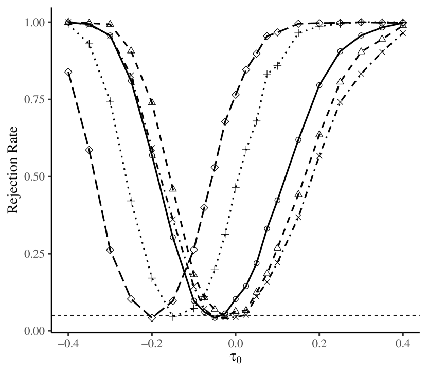
(a) constant $\pi_{0}$, $\mathrm{E}N_{z}=20$

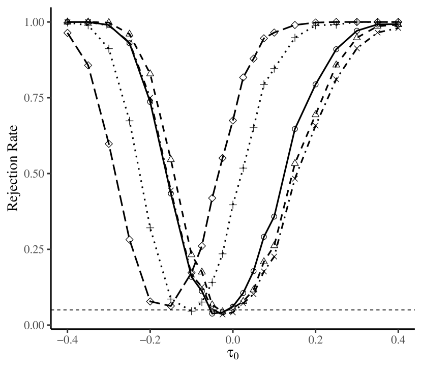
(b) constant $\pi_{0}$, $\mathrm{E}N_{z}=25$

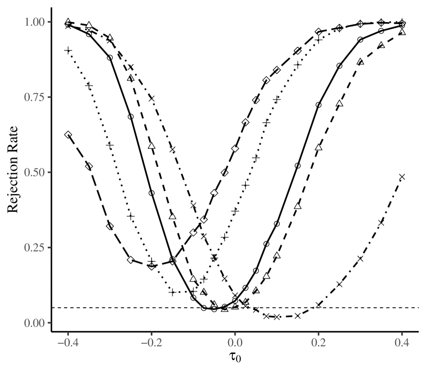
(c) heterogeneous $\pi_{0}$, $\mathrm{E}N_{z}=20$

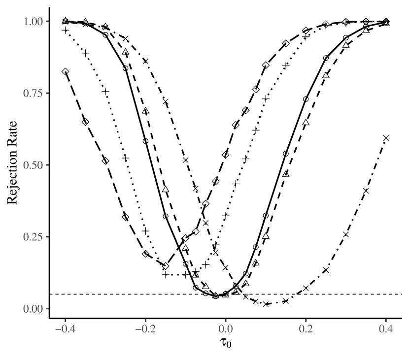
(d) heterogeneous $\pi_{0}$, $\mathrm{E}N_{z}=25$

Notes. Simulation results are based on 1000 replications using the DGP described in Section 4 with $K_{0}=2$. Panels (a) and (b) are with constant effects so that $\pi_{0}(X_{i})=\tau_{0}$. Panels (c) and (d) allow for covariate-dependent effects with $\pi_{0}(X_{i})=1-2X_{i}+\tau_{0}$. The power curves plot the rejection rate of testing $H_{0}:\tau_{0}=0$ at significance level $\alpha=0.05$. CIV denotes the categorical IV estimator with known $K_{0}$. “CIV” correspond to the proposed categorical IV estimator with $K=2$, “Oracle” denotes the infeasible oracle estimator $\tilde{\theta}^{K_{0}}$ with known optimal instrument, “TSLS” denotes the two-stage least squares estimator using the observed instruments, “LIML” denotes the limited information maximum likelihood estimator using the observed instruments, and “Lasso-IV (cv)” denotes IV estimator that use lasso to estimate the optimal instrument using a cross-validated penalty parameter.

5 Application to Returns to Schooling

This paper joins the large literature on many or weak instrument estimators using the Angrist and Krueger, (1991, AK91 hereafter) application as an empirical illustration (among many others, see, e.g., Bound et al.,, 1995; Angrist and Krueger,, 1995; Angrist et al.,, 1999; Donald and Newey,, 2001; Hansen et al.,, 2008; Angrist and Frandsen,, 2022; Mikusheva and Sun,, 2022). Despite the many applications of IV estimators to the AK91 setting, the purely categorical nature of the considered instruments is not commonly taken advantage of. I revisit the returns to schooling analysis of AK91 in a sample of 329,509 American men born between 1930 and 1939. The authors use quarter of birth (QOB) indicators as instruments for the highest grade completed. This approach is motivated by two arguments. First, quarter of birth is plausibly exogenous with other determinants of wages. Second, children born in later quarters attain the minimum dropout age after having completed more schooling. While the QOB instrument thus appears a valid approach to instrument for years of schooling, it averages over potential heterogeneity in educational policy. A larger number of categorical instruments arises when interactions between QOB and indicators for year of birth and place of birth (POB) are formed. These interactions capture the fact that mandatory schooling laws differ across cohorts and states. In particular, the interactions account for the possibility that two students born in the same QOB may differ on whether they can dropout depending on the particular policy in place in their state. I focus on interactions of QOB with the 51 values of POB to compare estimators in random subsamples of the original data.

The setting of AK91 is an interesting application of the CIV estimator proposed here as the economic motivation of the QOB-instrument directly suggests existence of a latent binary optimal instrument: A student’s dropout decision either is or is not constrained by the mandatory attendance law in place in their state. While it would thus be ideal to know of the specific educational policies across all states, the CIV estimator provides an approach to estimate this map from interactions of QOB and POB to the latent binary instrument that captures whether or not a student was constrained in their schooling decision. In particular, consider a sample $\{(Y_{i},D_{i},\text{QOB}_{i},\text{POB}_{i})\}_{i=1}^{n}$ of $n$ students with log-weekly wage $Y_{i}$, $D_{i}$ years of education, and born in $\text{QOB}_{i}$ and $\text{POB}_{i}$. The CIV estimator with $K=2$ directly applies if

$$\mathrm{E}[D_{i}|\text{QOB}_{i},\text{POB}_{i}]=m_{0}(\text{QOB}_{i},\text{POB}_{i})+\sum_{j=1}^{51}\mathbbm{1}_{j}(\text{POB}_{i})\pi_{0j},$$ (7)

where $m_{0}$ is the map to the optimal instrument in Assumption 4 (b), the optimal instrument captures the difference in schooling for a constrained or unconstrained student, and $(\pi_{0j})_{j=1}^{51}$ in the second term capture level-differences in years of schooling across states. Note that the restriction of $m_{0}$ to two support points implies that the expected increment in years of schooling implied by the constraint of a mandatory attendance law is constant across states. If there is additional heterogeneity in the first stage effect of being constrained, CIV with $K=2$ serves as an approximation to the optimal instrument estimator but remains root-$n$ normal at the cost of statistical efficiency (see Theorem 1).

Table 2 presents estimation results of the coefficient of log-weekly wage on years of schooling in the original AK91 data using eight estimators: OLS, TSLS, three CIV estimators with $K=2$, $K=3$, and $K=4$, LIML, and two specifications of the post-Lasso TSLS estimator proposed by Belloni et al., (2012). The two lasso-based IV estimators differ in how the indicators for the categorical instruments are constructed: While Lasso-IV (1) includes three QOB indicators (dropping the indicator for the first QOB) and 150 indicators for interactions between QOB and POB, Lasso-IV (2) directly includes 153 indicators for the interactions between the QOB and POB values. Lasso-IV (1) and Lasso-IV (2) thus differ in how they define the constant, or, “base-case”. Of course, such differences in indicator specification results in numerically identical estimates for any of the other considered estimators.

Column (6) of Table 2 provides estimation results using the full sample of 329,509 observations. In this sample size, TSLS, LIML, and all three CIV estimators provide qualitatively similar estimation results: All coefficient estimates are near 0.1 and statistically significant at a 5% nominal level. Similar performances of TSLS and the CIV estimators at this very large sample size are reassuring since one may reasonably expect the many instruments problem to be avoided given only the 150 excluded instruments, and closeness of the LIML estimator may suggest only little heterogeneity in the second stage effects. Among this set of estimators, the qualitative conclusions thus seem robust. In contrast, the results of the lasso-based IV estimators depend strongly on the specification of the indicators in the first stage. While Lasso-IV (1) is statistically insignificant, Lasso-IV (2) returns the largest point estimate paired with the smallest standard error of all considered IV estimators. Since the choice of indicator specification is often arbitrary, lasso-based IV estimation in this setting leaves the researcher with two qualitatively very different results. Much akin the approach of Donald and Newey, (2001) who consider an ordered list of instruments in increasing importance from which to choose from, applications of lasso-based estimators for categorical variables require careful consideration of the constructed sets of indicators.

The true coefficient in the AK91 application is unknown. To nevertheless provide some insights into the finite-sample trade-offs between the different estimators, I re-compute the estimators on random subsamples of the original data. Column (1)-(5) provide the corresponding mean coefficient and mean standard error estimates across 250 replications along with the median absolute difference to the corresponding full-sample coefficient estimate.

Compared to the TSLS estimator, CIV estimator with $K=2$ is slightly less biased towards OLS for smaller sample sizes while maintaining roughly equal deviations from its corresponding full-sample estimate, suggesting that $K=2$ provides some well-suited regularization to the first stage. For CIV with $K=3$ and $K=4$, estimates are slightly closer to the TSLS estimate further suggesting that the first stage model in (7) along with $K=2$ may indeed be a good approximation of the optimal instrument structure. In contrast to TSLS and the CIV estimators, the LIML estimator is highly variable for small and moderate sample sizes. Indeed, at 10% or 30% of the original data, the median absolute deviation of LIML is substantially larger. Finally, the two lasso-based estimators suffer from the differing qualitative conclusions for all sample sizes: While Lasso-IV (1) is highly variable in particular for small sample sizes, Lasso-IV (2) is very stable, statistically significant, and large. In addition, at smaller sample sizes, Lasso-IV (1) occasionally does not select any instruments in the first stage, resulting in non-defined estimates. In particular, Lasso-IV (1) does not select any instruments in 58% of replications when $n=32,950$, in 20% of replications when $n=98,852$, and in 11% of replications when $n=131,803$.

Table 2: Angrist and Krueger, (1991) Estimation Results

	$n=$	$32,950$	$98,852$	$131,803$	$197,705$	$296,558$	Full Sample
		(1)	(2)	(3)	(4)	(5)	(6)
OLS	Mean Coef.	0.067	0.067	0.067	0.067	0.067	0.067
	Mean S.E.	(0.001)	(0.001)	(0.001)	(0.0005)	(0.0004)	(0.0004)
	MAE	[0.001]	[0.0004]	[0.0002]	[0.0002]	[0.0001]	-
TSLS	Mean Coef.	0.073	0.083	0.091	0.095	0.098	0.099
	Mean S.E.	(0.015)	(0.014)	(0.012)	(0.011)	(0.011)	(0.010)
	MAE	[0.026]	[0.016]	[0.008]	[0.006]	[0.003]	-
CIV ($K=2$)	Mean Coef.	0.076	0.087	0.095	0.098	0.100	0.102
	Mean S.E.	(0.023)	(0.019)	(0.016)	(0.014)	(0.013)	(0.012)
	MAE	[0.026]	[0.016]	[0.01]	[0.007]	[0.004]	-
CIV ($K=3$)	Mean Coef.	0.073	0.084	0.093	0.096	0.099	0.109
	Mean S.E.	(0.019)	(0.016)	(0.014)	(0.013)	(0.012)	(0.012)
	MAE	[0.035]	[0.026]	[0.016]	[0.013]	[0.01]	-
CIV ($K=4$)	Mean Coef.	0.074	0.084	0.092	0.095	0.097	0.095
	Mean S.E.	(0.017)	(0.015)	(0.013)	(0.012)	(0.011)	(0.011)
	MAE	[0.021]	[0.012]	[0.007]	[0.006]	[0.004]	-
Lasso-IV (1)	Mean Coef.	0.090	0.079	0.088	0.093	0.094	0.091
	Mean S.E.	(0.429)	(0.306)	(0.153)	(0.107)	(0.078)	(0.061)
	MAE	[0.043]	[0.028]	[0.018]	[0.011]	[0.008]	-
Lasso-IV (2)	Mean Coef.	0.131	0.138	0.137	0.137	0.137	0.137
	Mean S.E.	(0.008)	(0.004)	(0.003)	(0.002)	(0.002)	(0.002)
	MAE	[0.007]	[0.002]	[0.001]	[0.001]	[0.0005]	-
LIML	Mean Coef.	0.355	0.117	0.118	0.115	0.115	0.115
	Mean S.E.	(13.918)	(0.025)	(0.018)	(0.015)	(0.013)	(0.012)
	MAE	[0.073]	[0.026]	[0.013]	[0.007]	[0.004]	-

• Notes. Subsampling estimation results are based on 250 replications. “Mean Coef.” and “Mean S.E.” denote the mean coefficient and standard error estimate across subsampling replications. “MAE” denotes the median absolute difference to the full sample coefficient estimate.“OLS”, “TSLS”, and “LIML” denote least squares, two-stage least squares, and limited information maximum likelihood, respectively. “CIV ($K=2$)”, “CIV ($K=3$)” , “CIV ($K=4$)” denotes the proposed categorical IV estimators restricted to 2, 3, and 4 support points in the first stage. “Lasso-IV (1)” and “Lasso-IV (2)” denote post-lasso IV estimators proposed by Belloni et al., (2012) using two indicator constructions: “Lasso-IV (1)” uses the set of indicators for QOB and the interaction terms QOB$\times$POB, “Lasso-IV (2)” uses the set of indicators for the fully interacted set QOB$\times$POB. Lasso-IV (1) does not select any instruments in 58% of replications when $n=32,950$, in 20% of replications when $n=98,852$, and in 11% of replications when $n=131,803$. The corresponding point estimates are omitted from computation of the summary statistics of Lasso-IV (1).

6 Conclusion

This paper considers estimation with categorical instrumental variables when the number of observations per category is relatively small. The proposed categorical instrumental variable estimator is motivated by a first-stage regularization assumption that restricts the unknown optimal instrument to have fixed finite support. In asymptotic regimes that allow the number of observations to grow at arbitrarily slow polynomial rate with the sample, I show that when the number of support points of the optimal instrument is known, CIV achieves the same asymptotic variance as the infeasible oracle two stage least squares estimator that presumes knowledge of the optimal instrument and is semiparametrically efficient under homoskedasticity. Further, under-specifying the number of support points maintains asymptotic normality but results in efficiency loss. A simulation exercise illustrates the finite sample performance of the proposed CIV estimator and highlights pitfalls associated with lasso-based IV estimators in the setting of categorical instruments. Further, the application to Angrist and Krueger, (1991) illustrates how the finite support assumption leveraged by CIV may be motivated in practice using the underlying economic setting.

The key advantage of the proposed CIV estimator is the appeal of the finite support assumption over alternative first stage regularization assumptions such as (approximate) sparsity in settings with categorical instruments. As showcased in the simulation and application, sparsity can have unintended implications in settings with categorical instruments with substantial practical consequences. In particular, the assumption leveraged in this paper does not restriction the proportion of observations across latent categories. CIV thus appears a suitable and easily applicable alternative to existing estimators in important empirical settings similar to Angrist and Krueger, (1991) or judge IV designs.

Appendix A Proofs

The proof of Theorem 1 and Corollary 1 proceeds in four steps: First, I begin the proof with a set of lemmas to characterize the asymptotic properties of the first stage estimator $\hat{m}_{K}^{(n)}$. The proof of lemmas 2-4 heavily leverages the arguments of Bonhomme and Manresa, (2015). Novel arguments provided here include the characterization of the approximation $m^{(n)}_{K}$ of $m^{(n)}_{0}$ for $K\leq K_{0}$ in Lemma 1 which leverages the dynamic programming characterization of KMeans in $\mathbbm{R}$ of Wang and Song, (2011), and accommodations to unbalanced categorical variables including Lemma 5. Second, I characterize the asymptotic distribution of $\hat{\theta}^{K}$. Third, I prove consistency of the covariance estimator $\hat{\Sigma}_{K}$ in Lemma 7. Finally, I prove semiparametric efficiency of $\hat{\theta}^{K_{0}}$ under homoskedasticity.

Notation. For notational brevity, the proof defines $Z\equiv Z^{(n)}$, $\mathcal{Z}\equiv\mathcal{Z}^{(n)}$, $m_{K}\equiv m_{K}^{(n)}$, and $\hat{m}_{K}^{(n)}\equiv\hat{m}_{K}$, omitting the explicit dependence on $n$.

A.1 Convergence of $\hat{m}_{K}$

I begin by highlighting two important properties of the optimal instrument $Z^{(0)}$. Note that by Assumption 2, it follows from the definition of the support of a random variable that

$$\exists\underline{p}>0:\>\Pr(Z^{(0)}=d_{z})\geq\underline{p},\forall d_{z}\in\mathcal{Z}^{(0)}.$$ (8)

Further, since $\mathcal{Z}^{(0)}$ is a finite collection of points in $\mathbbm{R}$,

$$\exists c>0:\>(d_{z}-\tilde{d}_{z})^{2}\geq c,\forall d_{z}\neq\tilde{d}_{z}\in\mathcal{Z}^{(0)}.$$ (9)

Lemma 1 shows that the approximation of $Z^{(0)}$ with $K\in\{2,\ldots,K_{0}\}$ unique support points also satisfies (8) and (9).

Lemma 1.

Let the assumptions of Theorem 1 hold. Then, $\forall K\in\{2,\ldots,K_{0}\}$, $m_{K}$ satisfies

1. $\Pr(m_{K}(Z)=\alpha)\geq\underline{p},\forall\alpha\in m_{K}(\mathcal{Z})$, and

2. $(\alpha-\tilde{\alpha})^{2}\geq c,\forall\alpha\neq\tilde{\alpha}\in m_{K}(\mathcal{Z}),$

where $\underline{p}$ and $c$ are positive constants from conditions (8) and (9).

Proof.

Note that by Assumption 2 (b) we have $Z^{(0)}=m_{0}(Z)$ so that the result follows directly for $K=K_{0}$ by Assumption 2. Further, note that $m_{K}$ is equivalently defined by

$$m_{K}\equiv\operatorname*{arg\,min}_{\begin{subarray}{c}m:\mathcal{Z}\to\mathcal{M}\\ |m(\mathcal{Z})|\leq K\end{subarray}}\>\mathrm{E}(m_{0}(Z)-m(Z))^{2}.$$

Let $\alpha^{0}_{1}\leq\ldots\leq\alpha^{0}_{K_{0}}$ and $\alpha^{K}_{1}\leq\ldots\leq\alpha^{K}_{K}$ denote the support points of $m_{0}(Z)$ and $m_{K}(Z)$, respectively, in non-decreasing order, and let $p^{0}_{1},\ldots,p^{0}_{K}$ and $p^{K}_{1},\ldots,p^{K}_{K}$ denote the corresponding point masses.

Let $G[k,M]$ denote the minimum objective function in the sub-problem of approximating the first $2\leq k\leq K_{0}$ support points of $m_{0}(Z)$ by $1<M\leq k$ clusters – i.e.,

$$G[k,M]\equiv\min_{\begin{subarray}{c}m:\mathcal{Z}\to\mathcal{M}\\ |m(\mathcal{Z})|\leq M\end{subarray}}\mathrm{E}\left[\left(m_{0}(Z)-m(Z)\right)^{2}\big{|}m_{0}(Z)\leq\alpha^{0}_{k}\right],$$

so that $G[K_{0},K]$ is the minimum objective function of the original problem. Now following the arguments of Wang and Song, (2011), let $M\leq j\leq k$ denote the smallest support point in the $M$th cluster of the solution to $G[k,M]$. Then $G[j-1,M-1]$ must be the minimum objective function of clustering the first $j-1$ support points into $M-1$ cluster as otherwise $G[k,M]$ would not be optimal. As a consequence, the problem admits the following sub-structure:

$$G[k,M]=\min_{M\leq j\leq k} \>\bigg{\{}G[j-1,M-1]\Pr(m_{0}(Z)\leq\alpha^{0}_{j-1}|m_{0}(Z)\leq\alpha^{0}_{k})$$

$$+\min_{a_{M}^{K}\in\mathbbm{M}}\bigg{[}\mathrm{E}\left[\left(m_{0}(Z)-a_{M}^{K}\right)^{2}\big{|}\alpha^{0}_{j}\leq m_{0}(Z)\leq\alpha^{0}_{k}\right]$$

$$\qquad\quad\quad\times\Pr(m_{0}(Z)\geq\alpha^{0}_{j}|m_{0}(Z)\leq\alpha^{0}_{k})\bigg{]}\bigg{\}},$$

for all $2\leq M\leq k\leq K_{0}$, where the second term characterizes the optimal within-cluster points. The desired properties of $m_{K}$ now follow directly from the sub-structure.

First, for any $\ell\geq 2$, we have

$$|\alpha^{K}_{\ell-1}-\alpha^{K}_{\ell}|\geq|\alpha^{0}_{j_{\ell}-1}-\alpha^{0}_{j_{\ell}}|\geq c,$$

where $j_{\ell}$ is the index of the smallest support point in the $\ell$th cluster and the second inequality follows from (8).

Second, it is clear from the sub-structure that support points are combined so that

$$\min\{p_{k}^{K}\}_{k=1}^{K}\geq\min\{p_{k}^{0}\}_{k=1}^{K_{0}}\geq\underline{p},$$

where the second inequality follows from (9). ∎

Note that, because $|\mathcal{Z}|$ is finite for every $n\in\mathbbm{N}$ by Assumption 1 and $m_{K}$ takes $K$ unique values, each such function $m:\mathcal{Z}\to\mathcal{M},|m(\mathcal{Z})|\leq K$ is fully characterized by a set of coefficients $(\alpha_{k})_{k=1}^{K}$ and a map $\gamma:\mathcal{Z}\to\{1,\ldots,K\}$. It is thus possible to re-cast $m_{K}$ as

$$(\alpha^{K},\gamma^{K})\equiv\operatorname*{arg\,min}_{(\alpha,\gamma)\in\mathcal{M}^{K}\times\Gamma^{K}}\>\mathrm{E}(Z^{(0)}-\alpha_{\gamma(Z)}))^{2}.$$

where $\Gamma^{K}=\{\gamma:\mathcal{Z}\to\{1,\ldots,K\}\}$ so that

$$m_{K}(z)=\alpha^{K}_{\gamma}(z),\>\forall z\in\mathcal{Z}.$$

Similarly, for the corresponding estimator $\hat{m}_{K}$ we have

$$(\hat{\alpha}^{K},\hat{\gamma}^{K})\equiv\operatorname*{arg\,min}_{(\alpha,\gamma)\in\mathcal{M}^{K}\times\Gamma^{K}}\>\mathbbm{E}_{n}(D-X^{\top}\hat{\pi}-\alpha_{\gamma(Z)})^{2},$$ (10)

so that

$$\hat{m}_{K}(z)=\hat{\alpha}^{K}_{\hat{\gamma}^{K}(z)},\>\forall z\in\mathcal{Z}.$$

This representation of $m_{K}$ and $\hat{m}_{K}$ follows the group fixed effects estimator of Bonhomme and Manresa, (2015). I adopt it here because it allows for separate analysis of estimation properties of the partition and the coefficients.

Lemma 2.

Let the assumptions of Theorem 1 hold. Then, $\forall K\in\{2,\ldots,K_{0}\}$, we have

$$\mathbbm{E}_{n}\left(m_{K}(Z)-\hat{\alpha}^{K}_{\hat{\gamma}^{K}(Z)}\right)^{2}=o_{p}(1).$$

Proof.

Fix an arbitrary $K\in\{2,\ldots,K_{0}\}$ and define

$$\hat{Q}_{K}(\alpha,\gamma,\pi)=\mathbbm{E}_{n}\left(D-\alpha_{\gamma(Z)}-X^{\top}\pi\right)^{2}=\mathbbm{E}_{n}\left(m_{K}(Z)+X^{\top}\pi_{0}+V_{K}-\alpha_{\gamma(Z)}-X^{\top}\pi\right)^{2}$$

and

$$\tilde{Q}_{K}(\alpha,\gamma,\pi)=\mathbbm{E}_{n}\left(m_{K}(Z)-\alpha_{\gamma(Z)}+X^{\top}(\pi_{0}-\pi)\right)^{2}+\mathbbm{E}_{n}V_{K}^{2},$$

where

$$V_{K}\equiv V+m_{0}(Z)-m_{K}(Z).$$

For any $(\alpha,\gamma)\in\mathcal{M}^{K}\times\Gamma^{K}$,

$$\hat{Q}_{K}(\alpha,\gamma,\hat{\pi})-\tilde{Q}_{K}(\alpha,\gamma,\hat{\pi}) =2\mathbbm{E}_{n}V_{K}(m_{0}(Z)-\alpha_{\gamma(Z)}+X^{\top}(\pi_{0}-\hat{\pi}))$$

$$=2\mathbbm{E}_{n}V_{K}m_{0}(Z)-2\mathbbm{E}_{n}V_{K}\alpha_{\gamma(Z)}+2\mathbbm{E}_{n}V_{K}X^{\top}(\pi_{0}-\hat{\pi})$$

$$=2\mathbbm{E}_{n}V_{K}m_{0}(Z)-2\mathbbm{E}_{n}V_{K}\alpha_{\gamma(Z)}+o_{p}(1),$$

where the last equation follows from Assumption 4 (a) and Assumption 5 (c). Further,

$$\mathbbm{E}_{n}V_{K}\alpha_{\gamma(Z)} =\mathbbm{E}_{n}\left[\sum_{z\in\mathcal{Z}}\mathbbm{1}_{z}(Z)V_{K}\alpha_{\gamma(z)}\right]=\frac{1}{K_{Z}}\sum_{z\in\mathcal{Z}}\alpha_{\gamma(z)}\left(\frac{K_{Z}}{n}\sum_{i=1}^{n}\mathbbm{1}_{z}(Z_{i})V_{iK}\right),$$

so by Cauchy-Schwarz

$$\left(\frac{1}{K_{Z}}\sum_{z\in\mathcal{Z}}\alpha_{\gamma(z)}\left(\frac{K_{Z}}{n}\sum_{i=1}^{n}\mathbbm{1}_{z}(Z_{i})V_{iK}\right)\right)^{2}\leq\left(\frac{1}{K_{Z}}\sum_{z\in\mathcal{Z}}\alpha_{\gamma(z)}^{2}\right)\left(\frac{1}{K_{Z}}\sum_{z\in\mathcal{Z}}\left(\frac{K_{Z}}{n}\sum_{i=1}^{n}\mathbbm{1}_{z}(Z_{i})V_{iK}\right)^{2}\right).$$

The first term is $O_{p}(1)$ by Assumption 5 (b). For the second term, we have

$$\frac{1}{K_{Z}}\sum_{z\in\mathcal{Z}}\left(\frac{K_{Z}}{n}\sum_{i=1}^{n}\mathbbm{1}_{z}(Z_{i})V_{iK}\right)^{2}=\frac{K_{Z}}{n^{2}}\sum_{z\in\mathcal{Z}}\sum_{i=1}^{n}\sum_{j=1}^{n}V_{iK}V_{jK}\mathbbm{1}_{z}(Z_{i})\mathbbm{1}_{z}(Z_{j}).$$

Taking expectations results in

$$\mathrm{E}\left[\frac{K_{Z}}{n^{2}}\sum_{z\in\mathcal{Z}}\sum_{i=1}^{n}\sum_{j=1}^{n}V_{iK}V_{jK}\mathbbm{1}_{z}(Z_{i})\mathbbm{1}_{z}(Z_{j})\right]$$

$$\overset{[1]}{=} \frac{K_{Z}}{n}\mathrm{E}V_{K}^{2}$$

$$\overset{[2]}{\leq} \frac{K_{Z}}{n}(L_{2}+\|m_{0}-m_{K}\|_{\infty}^{2})\overset{[3]}{=}o(1),$$

where [1] follows from Assumption 5 (d) and the fact that $\mathrm{E}V_{K}=0$, [2] follows from Assumption 3 (b) and Assumption 5 (a), and [3] is a consequence of Assumption 5 (b), Assumption 1 and the fact that $\sum_{z\in\mathcal{Z}}\Pr(Z=z)=1$ which implies $K_{Z}=o(n)$. It then follows that

$$\sup_{\begin{subarray}{c}(\alpha,\gamma)\in\mathcal{M}^{K}\times\Gamma^{K}\end{subarray}}\big{|}\hat{Q}_{K}(\alpha,\gamma,\hat{\pi})-\tilde{Q}_{K}(\alpha,\gamma,\hat{\pi})\big{|}=o_{p}(1).$$ (11)

Consider now

$$\begin{aligned} \tilde{Q}_{K}(\hat{\alpha}^{K},\hat{\gamma}^{K},\hat{\pi})&\overset{[1]}{=}\hat{Q}_{K}(\hat{\alpha}^{K},\hat{\gamma}^{K},\hat{\pi})+o_{p}(1)\overset{[2]}{\leq}\hat{Q}_{K}(\alpha^{K},\gamma^{K},\hat{\pi})+o_{p}(1)\overset{[3]}{=}\tilde{Q}_{K}(\alpha^{K},\gamma^{K},\hat{\pi})+o_{p}(1),\end{aligned}$$ (12)

where [1] and [3] follow from (11), and [2] follows from the definition of $(\hat{\alpha}^{K},\hat{\gamma}^{K})$.

The desired result then follows from

$$o_{p}(1) =\tilde{Q}_{K}(\hat{\alpha}^{K},\hat{\gamma}^{K},\hat{\pi})-\tilde{Q}_{K}(\alpha^{K},\gamma^{K},\hat{\pi})$$

$$=\mathbbm{E}_{n}(m_{K}(Z)-\hat{\alpha}^{K}_{\hat{\gamma}^{K}(Z)})^{2}+\mathbbm{E}_{n}(m_{K}(Z)-\hat{\alpha}^{K}_{\hat{\gamma}^{K}(Z)})(X^{\top}(\pi_{0}-\hat{\pi}))$$

$$=\mathbbm{E}_{n}(m_{K}(Z)-\hat{\alpha}^{K}_{\hat{\gamma}^{K}(Z)})^{2}+o_{p}(1),$$

where the last equality follows from Cauchy-Schwarz applied to the second term

$$\left(\mathbbm{E}_{n}(m_{K}(Z)-\hat{\alpha}^{K}_{\hat{\gamma}^{K}(Z)})(X^{\top}(\pi_{0}-\hat{\pi}))\right)^{2} =\mathbbm{E}_{n}(m_{K}(Z)-\hat{\alpha}^{K}_{\hat{\gamma}^{K}(Z)})^{2}\mathbbm{E}_{n}\|X\|^{2}\|\pi_{0}-\hat{\pi}\|^{2}$$

$$\overset{[1]}{=}O_{p}(1)o_{p}(1)=o_{p}(1),$$

where [1] follows from Assumption 4 (a) and Assumption 5 (b)-(c).

∎

Since the estimator $(\hat{\alpha}^{K},\hat{\gamma}^{K})$ of $m_{K}$ is invariant to relabeling of the coefficients $\hat{\alpha}^{K}$ and clustering $\hat{\gamma}^{K}$, it is useful to consider the Hausdorff distance $d_{H}$ in $\mathbbm{R}^{K}$ to characterize the asymptotic properties of the estimators $\hat{\alpha}^{K}$. In particular, define

$$d_{H}(a,b)^{2}=\max\bigg{\{} \max_{k\in\{1,\ldots,K\}}\left(\min_{\tilde{k}\in\{1,\ldots,K\}}\left(\alpha_{\tilde{k}}-b_{k}\right)^{2}\right),\max_{\tilde{k}\in\{1,\ldots,K\}}\left(\min_{k\in\{1,\ldots,K\}}\left(\alpha_{\tilde{k}}-b_{k}\right)^{2}\right)\bigg{\}}.$$

Define $\alpha^{K}=(\alpha_{1}^{K},\ldots,\alpha_{K}^{K})$ to be a vector of the $K$ support points of $m_{K}$ and let $\gamma^{K}$ be the corresponding clustering so that

$$m_{K}(Z)=\alpha^{K}_{\gamma^{K}(Z)}.$$

Lemma 3.

Let the assumptions of Theorem 1 hold. Then, $\forall K\in\{2,\ldots,K_{0}\}$,

$$d_{H}(\hat{\alpha}^{K},\alpha^{K})=o_{p}(1).$$

Proof.

The proof proceeds in two steps. I first show that for all $k\in\{1,\ldots,K\}$,

$$\min_{\tilde{k}\in\{1,\ldots,K\}}\left(\hat{\alpha}^{K}_{\tilde{k}}-\alpha^{K}_{k}\right)^{2}=o_{p}(1).$$ (13)

Let $k\in\{1,\ldots,K\}$. We have

$$\mathbbm{E}_{n}\left(\min_{\tilde{k}\in\{1,\ldots,K\}}\mathbbm{1}\{\gamma^{K}(Z)=k\}(\hat{\alpha}^{K}_{\tilde{k}}-\alpha^{K}_{k})^{2}\right)=\left(\mathbbm{E}_{n}\mathbbm{1}\{\gamma^{K}(Z)=k\}\right)\left(\min_{\tilde{k}\in\{1,\ldots,K\}}(\hat{\alpha}^{K}_{\tilde{k}}-\alpha^{K}_{k})^{2}\right).$$

Since the first term of the right-hand side is non-vanishing by Lemma 1 (a), it suffices to show that the left-hand side is $o_{p}(1)$ for all $k\in\{1,\ldots,K\}$. In particular,

$$\mathbbm{E}_{n}\left(\min_{\tilde{k}\in\{1,\ldots,K\}}\mathbbm{1}\{\gamma^{K}(Z)=k\}(\hat{\alpha}^{K}_{\tilde{k}}-\alpha^{K}_{k})^{2}\right)\leq \mathbbm{E}_{n}\left(\mathbbm{1}\{\gamma^{K}(Z)=k\}(\hat{\alpha}^{K}_{\hat{\gamma}^{K}(Z)}-\alpha^{K}_{k})^{2}\right)$$

$$\leq \mathbbm{E}_{n}(\hat{\alpha}^{K}_{\hat{\gamma}^{K}(Z)}-\alpha^{K}_{\gamma^{K}(Z)})^{2}$$

$$= \mathbbm{E}_{n}(\hat{\alpha}^{K}_{\hat{\gamma}^{K}(Z)}-m_{K}(Z))^{2}$$

$$= o_{p}(1),$$

where the final equality follows from Lemma 2.

Next, I show that for all $\tilde{k}\in\{1,\ldots,K\}$,

$$\min_{k\in\{1,\ldots,K\}}\left(\hat{\alpha}^{K}_{\tilde{k}}-\alpha^{K}_{k}\right)^{2}=o_{p}(1).$$ (14)

Define

$$\sigma_{K}(k)\equiv\operatorname*{arg\,min}_{\tilde{k}\in\{1,\ldots,K\}}\left(\hat{\alpha}^{K}_{\tilde{k}}-\alpha^{K}_{k}\right)^{2}.$$

By the triangle inequality, it holds that

$$\left|\hat{\alpha}^{K}_{\sigma_{K}(k)}-\hat{\alpha}^{K}_{\sigma_{K}(\tilde{k})}\right| \geq\left|\alpha^{K}_{k}-\alpha^{K}_{\tilde{k}}\right|-\left|\hat{\alpha}^{K}_{\sigma_{K}(k)}-\alpha^{K}_{k}\right|-\left|\hat{\alpha}^{K}_{\sigma_{K}(\tilde{k})}-\alpha^{K}_{\tilde{k}}\right|$$

where $\left|\hat{\alpha}^{K}_{\sigma_{K}(k)}-\alpha^{K}_{k}\right|$ and $\left|\hat{\alpha}^{K}_{\sigma_{K}(\tilde{k})}-\alpha^{K}_{\tilde{k}}\right|$ are $o_{p}(1)$ by the first result (13), and $\left|\alpha^{K}_{k}-\alpha^{K}_{\tilde{k}}\right|>0$ by Lemma 1 (b). Thus $\sigma_{K}(k)\neq\sigma_{K}(\tilde{k})$ with probability approaching one, implying that the inverse $\sigma_{K}^{-1}$ is well-defined.

Now, with probability approaching one, we have

$$\min_{k\in\{1,\ldots,K\}}\left(\hat{\alpha}^{K}_{\tilde{k}}-\alpha^{K}_{k}\right)^{2} \leq\left(\hat{\alpha}^{K}_{\tilde{k}}-\alpha^{K}_{\sigma_{K}^{-1}(\tilde{k})}\right)^{2}$$

$$\overset{[1]}{=}\min_{h\in\{1,\ldots,K\}}\left(\hat{\alpha}^{K}_{h}-\alpha^{K}_{\sigma_{K}^{-1}(\tilde{k})}\right)^{2}$$

$$\overset{[2]}{=}o_{p}(1),$$

where [1] follows from $\tilde{k}=\sigma_{K}(\sigma_{K}^{-1}(\tilde{k}))$, and [2] follows from the first result (13).

Combining (13) and (14) completes the proof.

∎

The proof of Lemma 3 shows that for every $K\in\{2,\ldots,K_{0}\}$ there exists a permutation $\sigma_{K}:\{1,\ldots,K\}\to\{1,\ldots,K\}$ such that $\left(\hat{\alpha}^{K}_{\sigma_{K}(k)}-\alpha^{K}_{k}\right)^{2}=o_{p}(1).$ It is thus possible take $\sigma_{K}(k)=k$ by simply relabeling the elements of $\hat{\alpha}^{K}$. The remainder of the proof adopts this convention.

Further, let an $\eta$-neighborhood around a vector $\alpha^{K}$ be defined as $\mathcal{N}_{\alpha^{K}}(\eta)\equiv\{\alpha\in\mathcal{M}^{K}:\|\alpha-\alpha^{K}\|<\eta\}.$

Lemma 4.

For $\eta>0$ small enough, we have for all $K\in\{2,\ldots,K_{0}\}$ and $\delta>0$

$$\sup_{(\alpha,\pi)\in\mathcal{N}_{(\alpha^{K},\pi^{0})}(\eta)}\mathbbm{E}_{n}\mathbbm{1}\{\hat{\gamma}^{K}(Z;\alpha,\pi)\not=\gamma^{K}(Z)\}=o_{p}(n^{-\delta}).$$

Proof.

Fix an arbitrary $K\in\{2,\ldots,K_{0}\}$.

From the definition of $\hat{\gamma}$ in (10), we have for all $k\in\{1,\ldots,K\},z\in\mathcal{Z}$,

$$\mathbbm{1}\{\hat{\gamma}^{K}(z;\alpha,\pi)=k\}\leq\mathbbm{1}\left\{\mathbbm{E}_{n}\mathbbm{1}_{z}(Z)(Y-\alpha_{k}-X^{\top}\pi)^{2}\leq\mathbbm{E}_{n}\mathbbm{1}_{z}(Z)(Y-\alpha_{\gamma^{K}(z)}-X^{\top}\pi)^{2}\right\}.$$

As a consequence,

$$\begin{aligned} &\mathbbm{E}_{n}\mathbbm{1}\{\hat{\gamma}^{K}(Z;\alpha,\pi)\not=\gamma^{K}(Z)\}\\ =&\sum_{k=1}^{K}\mathbbm{E}_{n}\mathbbm{1}\{\gamma^{K}(Z)\not=k\}\mathbbm{1}\{\hat{\gamma}^{K}(Z;\alpha,\pi)=k\}\\ \leq&\mathbbm{E}_{n}\sum_{k=1}^{K}M^{K}_{Zk}(\alpha,\pi),\end{aligned}$$ (15)

where for all $z\in\mathcal{Z}$ and $k\in\{1,\ldots,K\}$

$$M^{K}_{zk}(\alpha,\pi) \equiv\mathbbm{1}\{\gamma^{K}(Z)\not=k\}\mathbbm{1}\left\{\mathbbm{E}_{n}\mathbbm{1}_{z}(Z)(D-\alpha_{k}-X^{\top}\pi)^{2}\leq\mathbbm{E}_{n}\mathbbm{1}_{z}(Z)(D-\alpha_{\gamma^{K}(z)}-X^{\top}\pi)^{2}\right\}$$

$$=\mathbbm{1}\{\gamma^{K}(Z)\not=k\}$$

$$\qquad\times\mathbbm{1}\left\{\mathbbm{E}_{n}\mathbbm{1}_{z}(Z)\left(2D(\alpha_{\gamma^{K}(z)}-\alpha_{k})-(\alpha_{\gamma^{K}(z)}-\alpha_{k})(\alpha_{\gamma^{K}(z)}+\alpha_{k}+2X^{\top}\pi)\right)\leq 0\right\}$$

$$=\mathbbm{1}\{\gamma^{K}(Z)\not=k\}$$

$$\qquad\times\mathbbm{1}\left\{\mathbbm{E}_{n}\mathbbm{1}_{z}(Z)(\alpha_{\gamma^{K}(z)}-\alpha_{k})\left(V_{K}+\alpha_{\gamma^{K}(z)}^{K}-\frac{(\alpha_{\gamma^{K}(z)}+\alpha_{k})}{2}+X^{\top}(\pi^{0}-\pi))\right)\leq 0\right\},$$

where I have substituted for $D=\alpha^{K}_{\gamma^{K}(Z)}+X^{\top}\pi^{0}+V_{K}$ and rearranged terms for simplification.

Now, whenever $(\alpha,\pi)\in\mathcal{N}_{(\alpha^{K},\pi^{0})}(\eta),$ it is possible to bound $M^{K}_{zk}(\alpha,\pi)$ by a quantity that does not depend on $(\alpha,\pi)$. In particular, note that

$$M^{K}_{zk}(\alpha,\pi) \leq\max_{\tilde{k}\not=k}\mathbbm{1}\left\{\mathbbm{E}_{n}\mathbbm{1}_{z}(Z)(\alpha_{\tilde{k}}-\alpha_{k})\left(V_{K}+\alpha_{\tilde{k}}^{K}-\frac{\alpha_{\tilde{k}}+\alpha_{k}}{2}+X^{\top}(\pi^{0}-\pi)\right)\leq 0\right\}.$$

Further, using that $V_{K}=V+m_{0}(Z)-m_{K}(Z)=V+\alpha^{0}_{\gamma^{0}(Z)}-\alpha^{K}_{\gamma^{K}(Z)}$, we have by simple application of the triangle inequality

$$\begin{aligned} &\bigg{|}\mathbbm{E}_{n}\mathbbm{1}_{z}(Z)(\alpha_{\tilde{k}}-\alpha_{k})\left(V+\alpha_{\tilde{k}}^{K}-\frac{\alpha_{\tilde{k}}+\alpha_{k}}{2}+X^{\top}(\pi^{0}-\pi)+m_{0}(z)-m_{K}(z)\right)\\ &\quad-\mathbbm{E}_{n}\mathbbm{1}_{z}(Z)(\alpha^{K}_{\tilde{k}}-\alpha^{K}_{k})\left(V+\alpha_{\tilde{k}}^{K}-\frac{\alpha^{K}_{\tilde{k}}+\alpha^{K}_{k}}{2}\right)\bigg{|}\\ \leq&\left|\mathbbm{E}_{n}\mathbbm{1}_{z}(Z)\left[(\alpha_{\tilde{k}}-\alpha_{k})-(\alpha^{K}_{\tilde{k}}-\alpha^{K}_{k})\right]V\right|\\ &\quad+\left|\mathbbm{E}_{n}\mathbbm{1}_{z}(Z)\left[(\alpha_{\tilde{k}}-\alpha_{k})\left(\alpha_{\tilde{k}}^{K}-\frac{\alpha_{\tilde{k}}+\alpha_{k}}{2}\right)-(\alpha^{K}_{\tilde{k}}-\alpha^{K}_{k})\left(\alpha_{\tilde{k}}^{K}-\frac{\alpha^{K}_{\tilde{k}}+\alpha^{K}_{k}}{2}\right)\right]\right|\\ &\quad+\left|\mathbbm{E}_{n}\mathbbm{1}_{z}(Z)(\alpha_{\tilde{k}}-\alpha_{k})X^{\top}(\pi^{0}-\pi)\right|\\ &\quad+\left|\mathbbm{E}_{n}\mathbbm{1}_{z}(Z)(\alpha_{\tilde{k}}-\alpha_{k})\top(m_{0}(z)-m_{K}(z))\right|.\end{aligned}$$ (16)

For the first term in (16), it holds that

$$\left|\mathbbm{E}_{n}\mathbbm{1}_{z}(Z)\left[(\alpha_{\tilde{k}}-\alpha_{k})-(\alpha^{K}_{\tilde{k}}-\alpha^{K}_{k})\right]V\right|$$

$$\overset{[1]}{\leq} \left(\mathbbm{E}_{n}\mathbbm{1}_{z}(Z)\right)\left[(\alpha_{\tilde{k}}-\alpha_{k})-(\alpha^{K}_{\tilde{k}}-\alpha^{K}_{k})\right]\left(\frac{1}{\mathbbm{E}_{n}\mathbbm{1}_{z}(Z)}\mathbbm{E}_{n}\mathbbm{1}_{z}(Z)V^{2}\right)^{\frac{1}{2}}$$

$$\overset{[2]}{\leq} 2\left(\mathbbm{E}_{n}\mathbbm{1}_{z}(Z)\right)\sqrt{\eta}\left(\frac{1}{\mathbbm{E}_{n}\mathbbm{1}_{z}(Z)}\mathbbm{E}_{n}\mathbbm{1}_{z}(Z)V^{2}\right)^{\frac{1}{2}},$$

where [1] follows from Jensen’s inequality, and [2] follows from $\alpha\in\mathcal{N}_{\alpha^{K}}(\eta)$. Similarly, for the second term in (16), it holds that

$$\left|\mathbbm{E}_{n}\mathbbm{1}_{z}(Z)\left[(\alpha_{\tilde{k}}-\alpha_{k})\left(\alpha_{\tilde{k}}^{K}-\frac{\alpha_{\tilde{k}}+\alpha_{k}}{2}\right)-(\alpha^{K}_{\tilde{k}}-\alpha^{K}_{k})\left(\alpha_{\tilde{k}}^{K}-\frac{\alpha^{K}_{\tilde{k}}+\alpha^{K}_{k}}{2}\right)\right]\right|$$

$$= \frac{1}{2}\left(\mathbbm{E}_{n}\mathbbm{1}_{z}(Z)\right)\left|\left[\left(\alpha_{\tilde{k}}-\alpha_{k}\right)-\left(\alpha^{K}_{\tilde{k}}-\alpha^{K}_{k}\right)\right]\left(\alpha_{\tilde{k}}^{K}-\alpha^{K}_{k}\right)+\left(\alpha_{\tilde{k}}-\alpha_{k}\right)\left[(\alpha^{K}_{\tilde{k}}+\alpha^{K}_{k})-(\alpha_{\tilde{k}}+\alpha_{k})\right]\right|$$

$$\leq \frac{1}{2}\left(\mathbbm{E}_{n}\mathbbm{1}_{z}(Z)\right)\bigg{(}\left|\left[\left(\alpha_{\tilde{k}}-\alpha_{k}\right)-\left(\alpha^{K}_{\tilde{k}}-\alpha^{K}_{k}\right)\right]\left(\alpha_{\tilde{k}}^{K}-\alpha^{K}_{k}\right)+\left(\alpha^{K}_{\tilde{k}}-\alpha^{K}_{k}\right)\left[(\alpha^{K}_{\tilde{k}}+\alpha^{K}_{k})-(\alpha_{\tilde{k}}+\alpha_{k})\right]\right|$$

$$\quad+\left|\left(\alpha_{\tilde{k}}-\alpha_{k}\right)\left[(\alpha^{K}_{\tilde{k}}+\alpha^{K}_{k})-(\alpha_{\tilde{k}}+\alpha_{k})\right]-\left(\alpha^{K}_{\tilde{k}}-\alpha^{K}_{k}\right)\left[(\alpha^{K}_{\tilde{k}}+\alpha^{K}_{k})-(\alpha_{\tilde{k}}+\alpha_{k})\right]\right|\bigg{)}$$

$$\overset{[1]}{\leq} \left(\mathbbm{E}_{n}\mathbbm{1}_{z}(Z)\right)\left(|\alpha^{K}_{\tilde{k}}-\alpha^{K}_{k}|\sqrt{\eta}+2\eta\right)$$

$$\overset{[2]}{\leq} \left(\mathbbm{E}_{n}\mathbbm{1}_{z}(Z)\right)C_{1}\sqrt{\eta},$$

with $C_{1}\equiv|\alpha^{K}_{\tilde{k}}-\alpha^{K}_{k}|+2$ a constant independent of $\eta,n$ and $(\alpha,\pi)$, and where [1] follows from $\alpha\in\mathcal{N}_{\alpha^{K}}(\eta)$, and [2] follows from $\sqrt{\eta}\geq\eta$ for $\eta\in[0,1]$. Finally, using analogous arguments as above, the third term in (16) can be bounded by

$$\left|\mathbbm{E}_{n}\mathbbm{1}_{z}(Z)(\alpha_{\tilde{k}}-\alpha_{k})X^{\top}(\pi^{0}-\pi)\right|\leq\left(\mathbbm{E}_{n}\mathbbm{1}_{z}(Z)\right)C_{2}\sqrt{\eta}\left(\frac{1}{\mathbbm{E}_{n}\mathbbm{1}_{z}(Z)}\mathbbm{E}_{n}\mathbbm{1}_{z}(Z)\|X\|^{2}\right),$$

where $C_{2}$ is a constant independent of $\eta,n$ and $(\alpha,\pi)$. And finally, the fourth term in (16) can be bounded by

$$\left|\mathbbm{E}_{n}\mathbbm{1}_{z}(Z)(\alpha_{\tilde{k}}-\alpha_{k})\top(m_{0}(z)-m_{K}(z))\right|\leq\left(\mathbbm{E}_{n}\mathbbm{1}_{z}(Z)\right)C_{3}\sqrt{\eta}\|m_{0}-m_{K}\|_{\infty},$$

where $C_{3}$ is a constant independent of $\eta,n$ and $(\alpha,\pi)$.

Therefore,

$$\begin{aligned} M^{K}_{zk}(\alpha,\pi)&\leq\max_{\tilde{k}\not=k}\mathbbm{1}\bigg{\{}\mathbbm{E}_{n}\mathbbm{1}_{z}(Z)(\alpha^{K}_{\tilde{k}}-\alpha^{K}_{k})\left(V+\alpha_{\tilde{k}}^{K}-\frac{\alpha^{K}_{\tilde{k}}+\alpha^{K}_{k}}{2}\right)\\ &\qquad\quad\leq 2\left(\mathbbm{E}_{n}\mathbbm{1}_{z}(Z)\right)\sqrt{\eta}\left(\frac{1}{\mathbbm{E}_{n}\mathbbm{1}_{z}(Z)}\mathbbm{E}_{n}\mathbbm{1}_{z}(Z)V^{2}\right)^{\frac{1}{2}}+\left(\mathbbm{E}_{n}\mathbbm{1}_{z}(Z)\right)C_{1}\sqrt{\eta}\\ &\qquad\qquad+\left(\mathbbm{E}_{n}\mathbbm{1}_{z}(Z)\right)C_{2}\sqrt{\eta}\left(\frac{1}{\mathbbm{E}_{n}\mathbbm{1}_{z}(Z)}\mathbbm{E}_{n}\mathbbm{1}_{z}(Z)\|X\|^{2}\right)\\ &\qquad\qquad+\left(\mathbbm{E}_{n}\mathbbm{1}_{z}(Z)\right)C_{3}\sqrt{\eta}\|m_{0}-m_{K}\|_{\infty}\bigg{\}}\\ &=\max_{\tilde{k}\not=k}\mathbbm{1}\bigg{\{}\frac{1}{\mathbbm{E}_{n}\mathbbm{1}_{z}(Z)}\mathbbm{E}_{n}\mathbbm{1}_{z}(Z)V(\alpha^{K}_{\tilde{k}}-\alpha^{K}_{k})\\ &\qquad\quad\leq 2\sqrt{\eta}\left(\frac{1}{\mathbbm{E}_{n}\mathbbm{1}_{z}(Z)}\mathbbm{E}_{n}\mathbbm{1}_{z}(Z)V^{2}\right)^{\frac{1}{2}}+C_{1}\sqrt{\eta}\\ &\qquad\qquad+C_{2}\sqrt{\eta}\left(\frac{1}{\mathbbm{E}_{n}\mathbbm{1}_{z}(Z)}\mathbbm{E}_{n}\mathbbm{1}_{z}(Z)\|X\|^{2}\right)\\ &\qquad\qquad+C_{3}\sqrt{\eta}\|m_{0}-m_{K}\|_{\infty}-\frac{1}{2}\left(\alpha^{K}_{\tilde{k}}-\alpha^{K}_{k}\right)^{2}\bigg{\}},\end{aligned}$$ (17)

where the right-hand side does not depend on $(\alpha,\pi)$.

Hence, for $\eta<1$ we have

$$\sup_{(\alpha,\pi)\in\mathcal{N}_{(\alpha^{K},\pi^{0})}(\eta)}M^{K}_{zk}(\alpha,\pi)\leq\tilde{M}^{K}_{zk},$$

where $\tilde{M}^{K}_{zk}$ denotes the final term in (17). Combining with (15) then implies

$$\sup_{(\alpha,\pi)\in\mathcal{N}_{(\alpha^{K},\pi^{0})}(\eta)}\mathbbm{E}_{n}\mathbbm{1}\{\hat{\gamma}^{K}(Z;\alpha,\pi)\not=\gamma^{K}(Z)\}\leq\sum_{k=1}^{K}\mathbbm{E}_{n}\tilde{M}^{K}_{Zk},$$

and therefore for any $\epsilon>0$ and $\delta>0$,

$$\Pr\left(\sup_{(\alpha,\pi)\in\mathcal{N}_{(\alpha^{K},\pi^{0})}(\eta)}\mathbbm{E}_{n}\mathbbm{1}\{\hat{\gamma}^{K}(Z;\alpha,\pi)\not=\gamma^{K}(Z)\}>\epsilon n^{-\delta}\right)$$

$$\leq \Pr\left(\sum_{k=1}^{K}\mathbbm{E}_{n}\tilde{M}^{K}_{Zk}>\epsilon n^{-\delta}\right)$$

$$\overset{[1]}{\leq} \frac{\mathrm{E}\left[\sum_{k=1}^{K}\mathbbm{E}_{n}\tilde{M}^{K}_{Zk}\right]}{\epsilon n^{-\delta}}$$

$$\leq \frac{\sum_{k=1}^{K}\mathbbm{E}_{n}\Pr(\tilde{M}^{K}_{Zk}=1)}{\epsilon n^{-\delta}}$$

where [1] follows from Markov’s inequality. It thus suffices to show that $\forall z\in\mathcal{Z}$, $k\in\{1,\ldots,K\}$, and $\delta>0$,

$$\Pr\left(\tilde{M}^{K}_{zk}=1\right)=o(n^{-\delta}).$$ (18)

For this purpose, let $L^{K}=\max\{L_{1},\sqrt{L_{1}},\|m_{0}-m_{K}\|_{\infty}\}$ and consider

$$\begin{aligned} \Pr\left(\tilde{M}^{K}_{zk}\right)&\overset{[1]}{\leq}\sum_{\tilde{k}\neq k}\Pr\bigg{(}\frac{1}{\mathbbm{E}_{n}\mathbbm{1}_{z}(Z)}\mathbbm{E}_{n}\mathbbm{1}_{z}(Z)V(\alpha^{K}_{\tilde{k}}-\alpha^{K}_{k})\\ &\qquad\quad\leq 2\sqrt{\eta}\left(\frac{1}{\mathbbm{E}_{n}\mathbbm{1}_{z}(Z)}\mathbbm{E}_{n}\mathbbm{1}_{z}(Z)V^{2}\right)^{\frac{1}{2}}+C_{1}\sqrt{\eta}\\ &\qquad\qquad+C_{2}\sqrt{\eta}\left(\frac{1}{\mathbbm{E}_{n}\mathbbm{1}_{z}(Z)}\mathbbm{E}_{n}\mathbbm{1}_{z}(Z)\|X\|^{2}\right)\\ &\qquad\qquad+C_{3}\sqrt{\eta}\|m_{0}-m_{K}\|_{\infty}-\frac{1}{2}\left(\alpha^{K}_{\tilde{k}}-\alpha^{K}_{k}\right)^{2}\bigg{)}\\ &\overset{[2]}{\leq}\sum_{\tilde{k}\neq k}\Pr\bigg{(}\frac{1}{\mathbbm{E}_{n}\mathbbm{1}_{z}(Z)}\mathbbm{E}_{n}\mathbbm{1}_{z}(Z)V(\alpha^{K}_{\tilde{k}}-\alpha^{K}_{k})\leq\sqrt{\eta}(C_{1}+L^{K}(2+JC_{2}+C_{3}))-\frac{1}{2}\left(\alpha^{K}_{\tilde{k}}-\alpha^{K}_{k}\right)^{2}\bigg{)}\\ &\qquad\quad+K\Pr\left(\frac{1}{\mathbbm{E}_{n}\mathbbm{1}_{z}(Z)}\mathbbm{E}_{n}\mathbbm{1}_{z}(Z)V^{2}>L^{K}\right)\\ &\qquad\quad+K\Pr\left(\frac{1}{\mathbbm{E}_{n}\mathbbm{1}_{z}(Z)}\mathbbm{E}_{n}\mathbbm{1}_{z}(Z)\|X\|^{2}>JL^{K}\right)\\ &\qquad\quad+K\Pr\left(\|m_{0}-m_{K}\|_{\infty}>L^{K}\right),\end{aligned}$$ (19)

where [1] follows from the union bound, and [2] follows from the triangle inequality. I now consider each term separately.

Focusing on the first term, fix $\eta\geq 0$ such that $\eta\leq\min\{1,\tilde{\eta}^{K}\}$ where

$$\tilde{\eta}^{K}<\left(\frac{c}{C_{1}+L^{K}(2+JC_{2}+C_{3})}\right)^{2}$$

with $c$ defined by (8). Denote

$$\tilde{c}_{\tilde{k},k}\equiv\sqrt{\eta}(C_{1}+L^{K}(2+JC_{2}+C_{3}))-\frac{1}{2}\left(\alpha^{K}_{\tilde{k}}-\alpha^{K}_{k}\right)^{2}.$$

Note that the choice of $\eta$ above implies that $\tilde{c}_{\tilde{k},k}<0$ for all combinations $\tilde{k}\neq k$. Further, fix $\tilde{\lambda}>0$ such that $\tilde{\lambda}<\lambda_{z}$ as defined by Assumption 1 (a) and consider

$$\begin{aligned} &\Pr\bigg{(}\frac{1}{\sum_{i=1}^{n}\mathbbm{1}_{z}(Z_{i})}\sum_{i=1}^{n}\mathbbm{1}_{z}(Z_{i})V_{i}(\alpha^{K}_{\tilde{k}}-\alpha^{K}_{g})\leq\tilde{c}_{\tilde{k},k}\bigg{)}\\ =&\Pr\bigg{(}\frac{1}{\sum_{i=1}^{n}\mathbbm{1}_{z}(Z_{i})}\sum_{i=1}^{n}\mathbbm{1}_{z}(Z_{i})V_{i}(\alpha^{K}_{\tilde{k}}-\alpha^{K}_{k})\leq\tilde{c}_{\tilde{k},k}\bigg{|}\sum_{i=1}^{n}\mathbbm{1}_{z}(Z_{i})>n^{\tilde{\lambda}}\bigg{)}\Pr\left(\sum_{i=1}^{n}\mathbbm{1}_{z}(Z_{i})>n^{\tilde{\lambda}}\right)\\ &+\Pr\bigg{(}\frac{1}{\sum_{i=1}^{n}\mathbbm{1}_{z}(Z_{i})}\sum_{i=1}^{n}\mathbbm{1}_{z}(Z_{i})V_{i}(\alpha^{K}_{\tilde{k}}-\alpha^{K}_{k})\leq\tilde{c}_{\tilde{k},k}\bigg{|}\sum_{i=1}^{n}\mathbbm{1}_{z}(Z_{i})\leq n^{\tilde{\lambda}}\bigg{)}\Pr\left(\sum_{i=1}^{n}\mathbbm{1}_{z}(Z_{i})\leq n^{\tilde{\lambda}}\right)\\ \leq&\Pr\bigg{(}\frac{1}{\sum_{i=1}^{n}\mathbbm{1}_{z}(Z_{i})}\sum_{i=1}^{n}\mathbbm{1}_{z}(Z_{i})V_{i}(\alpha^{K}_{\tilde{k}}-\alpha^{K}_{k})\leq\tilde{c}_{\tilde{k},k}\bigg{|}\sum_{i=1}^{n}\mathbbm{1}_{z}(Z_{i})>n^{\tilde{\lambda}}\bigg{)}\\ &+\Pr\left(\sum_{i=1}^{n}\mathbbm{1}_{z}(Z_{i})\leq n^{\tilde{\lambda}}\right),\end{aligned}$$ (20)

where the inequality follows from probabilities being bounded by 1. For the first term, it holds for any $\delta>0$ that

$$\begin{aligned} &\Pr\bigg{(}\frac{1}{\sum_{i=1}^{n}\mathbbm{1}_{z}(Z_{i})}\sum_{i=1}^{n}\mathbbm{1}_{z}(Z_{i})V_{i}(\alpha^{K}_{\tilde{k}}-\alpha^{K}_{k})\leq\tilde{c}_{\tilde{k},k}\>\bigg{|}\sum_{i=1}^{n}\mathbbm{1}_{z}(Z_{i})>n^{\tilde{\lambda}}\bigg{)}\\ \overset{[1]}{=}&\Pr\bigg{(}\frac{1}{N_{z}}\sum_{i=1}^{N_{z}}V_{iz}(\alpha^{K}_{\tilde{k}}-\alpha^{K}_{k})\leq\tilde{c}_{\tilde{k},k}\>\bigg{|}N_{z}>n^{\tilde{\lambda}}\bigg{)}\\ \overset{[2]}{\leq}&\Pr\bigg{(}\left|\frac{1}{N_{z}}\sum_{i=1}^{N_{z}}V_{iz}\right|\geq\frac{|\tilde{c}_{\tilde{k},k}|}{|\alpha^{K}_{\tilde{k}}-\alpha^{K}_{k}|}\>\bigg{|}N_{z}>n^{\tilde{\lambda}}\bigg{)}\\ \overset{[3]}{\leq}&\Pr\bigg{(}\left|\frac{1}{\lfloor n^{\tilde{\lambda}}\rfloor}\sum_{i=1}^{\lfloor n^{\tilde{\lambda}}\rfloor}V_{iz}\right|\geq\frac{|\tilde{c}_{\tilde{k},k}|}{|\alpha^{K}_{\tilde{k}}-\alpha^{K}_{k}|}\>\bigg{)}\\ \overset{[4]}{=}&o(n^{-\delta}),\end{aligned}$$ (21)

where [1] takes $V_{iz}\equiv(V_{i}|Z_{i}=z)$ and $N_{z}\equiv\sum_{i=1}^{n}\mathbbm{1}_{z}(Z_{i})$, [2] follows from $\tilde{c}_{\tilde{k},k}<0$ and the fact that $|\alpha^{K}_{\tilde{k}}-\alpha^{K}_{k}|>0,\forall\tilde{k}\neq k$ by Lemma 1 (b), and [3] follows from $\Pr(|\frac{1}{n}\sum_{i=1}^{n}V_{iz}|\geq b)\leq\Pr(|\frac{1}{\tilde{n}}\sum_{i=1}^{\tilde{n}}V_{iz}|\geq b),\forall\tilde{n}\leq n,b>0$, and $N_{z}\mathchoice{\mathrel{\hbox to0.0pt{$\displaystyle\perp$\hss}\mkern 2.0mu{\displaystyle\perp}}}{\mathrel{\hbox to0.0pt{$\textstyle\perp$\hss}\mkern 2.0mu{\textstyle\perp}}}{\mathrel{\hbox to0.0pt{$\scriptstyle\perp$\hss}\mkern 2.0mu{\scriptstyle\perp}}}{\mathrel{\hbox to0.0pt{$\scriptscriptstyle\perp$\hss}\mkern 2.0mu{\scriptscriptstyle\perp}}}(\sum_{i=1}^{\lfloor n^{\tilde{\lambda}}\rfloor}V_{iz})$. Finally, [4] follows by application of Lemma B.5 in Bonhomme and Manresa, (2015) where I take $T\equiv\lfloor n^{\tilde{\lambda}}\rfloor$, $z_{t}\equiv V_{iz}$, and $z\equiv\frac{|\tilde{c}_{\tilde{k},k}|}{|\alpha^{K}_{\tilde{k}}-\alpha^{K}_{k}|}.$ The lemma applies by Assumption 4 (b) and Assumption 5 (d).

To bound the second term in (20), I prove a simple concentration inequality in Lemma 5, whose application implies for any $\delta>0$,

$$\Pr\left(\sum_{i=1}^{n}\mathbbm{1}_{z}(Z_{i})\leq n^{a_{z}\tilde{\lambda}}\right)=o(n^{-\delta}),\quad\forall z\in\operatorname*{supp}Z.$$ (22)

Lemma 5.

Let $X_{n}$ be a Binomial random variable with $n$ trials and success probability $p_{n}=an^{\lambda-1}$ for fixed $a>0$ and $\lambda\in(0,1)$. Then, $\forall\delta>0$ and $\tilde{\lambda}>0:\lambda>\tilde{\lambda},$

$$\Pr\left(X_{n}\leq an^{\tilde{\lambda}}\right)=o(n^{-\delta}).$$

Proof.

By Chernoff’s inequality,

$$\Pr\left(X_{n}\leq an^{\tilde{\lambda}}\right)$$

$$\leq \exp\left\{-n\left[an^{\tilde{\lambda}-1}\log\left(\frac{an^{\tilde{\lambda}-1}}{an^{\lambda-1}}\right)+\left(1-an^{\tilde{\lambda}-1}\right)\log\left(\frac{1-an^{\tilde{\lambda}-1}}{1-an^{\lambda-1}}\right)\right]\right\}$$

$$= \exp\left\{-n\left[-an^{\tilde{\lambda}-1}(\lambda-\tilde{\lambda})\log(n)+\left(1-an^{\tilde{\lambda}-1}\right)\left(\log\left(1-an^{\tilde{\lambda}-1}\right)-\log\left(1-an^{\lambda-1}\right)\right)\right]\right\}.$$

It is possible to bound the terms involving the logarithm via the following simple inequalities:

$$\log(n)\leq\gamma(n^{1/\gamma}-1),\quad \forall n,\gamma>0,$$

$$\frac{-x}{1-x}\leq\log(1-x)\leq-x,\quad \forall x\in[0,1).$$

Therefore, fixing $\gamma>0:\lambda>\tilde{\lambda}+\frac{1}{\gamma}$,

$$\Pr\left(X_{n}\leq an^{\tilde{\lambda}}\right)$$

$$\leq \exp\left\{-n\left[-an^{\tilde{\lambda}-1}(\lambda-\tilde{\lambda})\gamma\left(n^{1/\gamma}-1\right)+\left(1-an^{\tilde{\lambda}-1}\right)\left(an^{\lambda-1}-\frac{an^{\tilde{\lambda}-1}}{1-an^{\tilde{\lambda}-1}}\right)\right]\right\}$$

$$= \exp\left\{-\left[an^{\lambda}+an^{\tilde{\lambda}}(\lambda-\tilde{\lambda})\gamma-an^{\tilde{\lambda}+1/\gamma}(\lambda+\tilde{\lambda})\gamma-a^{2}n^{\lambda-\tilde{\lambda}-1}-an^{\tilde{\lambda}}\right]\right\}$$

$$= \exp\left\{-n^{\lambda}\left[a+an^{\tilde{\lambda}-\lambda}(\lambda-\tilde{\lambda})\gamma-an^{\tilde{\lambda}+1/\gamma-\lambda}(\lambda-\tilde{\lambda})\gamma-a^{2}n^{\tilde{\lambda}-1}-an^{\tilde{\lambda}-\lambda}\right]\right\},$$

where the term in brackets tends to $a>0$ as $n\to\infty$. Finally, note that for any $\delta,\lambda>0$,

$$\exp\left\{-n^{\lambda}\right\}=o(n^{-\delta}),$$

which completes the proof.

∎

Combining (20)-(22) then implies for any $\delta>0$,

$$\Pr\bigg{(}\frac{1}{\sum_{i=1}^{n}\mathbbm{1}_{z}(Z_{i})}\sum_{i=1}^{n}\mathbbm{1}_{z}(Z_{i})V_{i}(\alpha^{K}_{\tilde{k}}-\alpha^{K}_{k})\leq\tilde{c}_{\tilde{k},k}\bigg{)}=o(n^{-\delta}).$$ (23)

Focusing now on the second term in (19) and following similar arguments as before, we have for any $\delta>0$

$$\Pr\left(\frac{1}{\sum_{i=1}^{n}\mathbbm{1}_{z}(Z_{i})}\sum_{i=1}^{n}\mathbbm{1}_{z}(Z_{i})V_{i}^{2}>L^{K}\right)$$

$$\leq \Pr\left(\frac{1}{\lfloor n^{\lambda-\tilde{\lambda}}\rfloor}\sum_{i=1}^{\lfloor n^{\lambda-\tilde{\lambda}}\rfloor}V_{iz}^{2}>L^{K}\right)+\Pr\left(\sum_{i=1}^{n}\mathbbm{1}_{z}(Z_{i})\leq n^{\lambda-\tilde{\lambda}}\right)$$

$$\leq \Pr\left(\left|\frac{1}{\lfloor n^{\lambda-\tilde{\lambda}}\rfloor}\sum_{i=1}^{\lfloor n^{\lambda-\tilde{\lambda}}\rfloor}V_{iz}^{2}-\mathrm{E}V_{z}^{2}\right|>L^{K}-\mathrm{E}V_{z}^{2}\right)+o(n^{-\delta}).$$

We can again apply Lemma B.5 in Bonhomme and Manresa, (2015) where I take $T\equiv\lfloor n^{\tilde{\lambda}}\rfloor$, $z_{t}\equiv V^{2}_{iz}-\mathrm{E}V^{2}_{z}$, and $z\equiv L^{K}-\mathrm{E}V^{2}_{z}$. Note that $L^{K}-\mathrm{E}V^{2}_{z}>0$ is implied by Assumption 4 (a). As a consequence, for any $\delta>0$

$$\Pr\left(\frac{1}{\sum_{i=1}^{n}\mathbbm{1}_{z}(Z_{i})}\sum_{i=1}^{n}\mathbbm{1}_{z}(Z_{i})V_{i}^{2}>L^{K}\right)=o(n^{-\delta}).$$ (24)

Similarly for the third term in (19) we have for any $\delta>0$

$$\Pr\left(\frac{1}{\sum_{i=1}^{n}\mathbbm{1}_{z}(Z_{i})}\sum_{i=1}^{n}\mathbbm{1}_{z}(Z_{i})\|X_{i}\|^{2}>JL^{K}\right)$$

$$\leq \Pr\left(\frac{1}{\lfloor n^{\lambda-\tilde{\lambda}}\rfloor}\sum_{i=1}^{\lfloor n^{\lambda-\tilde{\lambda}}\rfloor}\|X_{iz}\|^{2}>JL^{K}\right)+o(n^{-\delta})$$

$$\leq \Pr\left(\exists j\in\{1,\ldots,J\}:\>\frac{1}{\lfloor n^{\lambda-\tilde{\lambda}}\rfloor}\sum_{i=1}^{\lfloor n^{\lambda-\tilde{\lambda}}\rfloor}X_{ijz}^{2}>L^{K}\right)+o(n^{-\delta})$$

$$\leq \sum_{j=1}^{J}\Pr\left(\frac{1}{\lfloor n^{\lambda-\tilde{\lambda}}\rfloor}\sum_{i=1}^{\lfloor n^{\lambda-\tilde{\lambda}}\rfloor}X_{ijz}^{2}>L^{K}\right)+o(n^{-\delta})$$

$$\leq \sum_{j=1}^{J}\Pr\left(\left|\frac{1}{\lfloor n^{\lambda-\tilde{\lambda}}\rfloor}\sum_{i=1}^{\lfloor n^{\lambda-\tilde{\lambda}}\rfloor}X_{ijz}^{2}-\mathrm{E}X_{jz}^{2}\right|>L^{K}-\mathrm{E}X_{jz}^{2}\right)+o(n^{-\delta}).$$

We can then again apply Lemma B.5 in Bonhomme and Manresa, (2015) where I take $T\equiv\lfloor n^{\tilde{\lambda}}\rfloor$, $z_{t}\equiv X_{ijz}^{2}-\mathrm{E}X_{jz}^{2}$, and $z\equiv L^{K}-\mathrm{E}X_{jz}^{2}$. Note that $L^{K}-\mathrm{E}X_{jz}^{2}>0$ is implied by Assumption 4 (a). The lemma applies by Assumption 4 (c) and Assumption 5 (d). As a consequence, for any $\delta>0$

$$\Pr\left(\frac{1}{\sum_{i=1}^{n}\mathbbm{1}_{z}(Z_{i})}\sum_{i=1}^{n}\mathbbm{1}_{z}(Z_{i})\|X_{i}\|^{2}>JL^{K}\right)=o(n^{-\delta}).$$ (25)

Finally, not that for the fourth term in (19) we simply have $\Pr\left(\|m_{0}-m_{K}\|_{\infty}>L^{K}\right)=0$ by definition of $L^{K}$. Combining with (19), (23), (24), and (25) shows (18) and thus completes the proof.

∎

Next, I show that $\hat{m}_{K}$ converges at exponential rate to the infeasible least squares estimator of $D-X^{\top}\hat{\pi}$ on the set of indicators $\{\mathbbm{1}_{k}(\gamma^{K}(Z)\}_{k=1}^{K}$. In particular, for $K\in\mathbbm{N}$, define

$$\tilde{\alpha}^{K}\equiv\operatorname*{arg\,min}_{\alpha\in\mathcal{M}^{K}}\>\mathbbm{E}_{n}(D-X^{\top}\hat{\pi}-\alpha_{\gamma^{K}(Z)})^{2},$$ (26)

with $\hat{\pi}$ being a consistent first-step estimator for $\theta_{0}$.

Lemma 6.

Let the assumptions of Theorem 1 hold. Then, for all $K\in\{2,\ldots,K_{0}\}$ and $\delta>0$,

$$\mathbbm{E}_{n}(\hat{\alpha}^{K}_{\hat{\gamma}^{K}(Z)}-\tilde{\alpha}^{K}_{\gamma^{K}(Z)})^{2}=o_{p}(n^{-\delta}).$$

Proof.

Fix an arbitrary $K\in\{2,\ldots,K_{0}\}$. Define

$$\bar{Q}(\alpha,\pi)\equiv\mathbbm{E}_{n}(D-X^{\top}\pi-\alpha_{\gamma^{K}(Z)})^{2},\qquad\text{and}\qquad\hat{Q}(\alpha,\pi)\equiv\mathbbm{E}_{n}(D-X^{\top}\pi-\alpha_{\hat{\gamma}^{K}(Z;\alpha,\pi)})^{2}.$$

For $\eta$ satisfying the condition of Lemma 4, it holds for any $\delta>0$ that

$$\sup_{(\alpha,\pi)\in\mathcal{N}_{(\alpha^{K},\pi^{0})}(\eta)}\>\left|\bar{Q}(\alpha,\pi)-\hat{Q}(\alpha,\pi)\right|$$

$$= \sup_{(\alpha,\pi)\in\mathcal{N}_{(\alpha^{K},\pi^{0})}(\eta)}\>\bigg{|}\mathbbm{E}_{n}\mathbbm{1}\{\hat{\gamma}^{K}(Z;\alpha,\pi)\not=\gamma^{K}(Z)\}(D-X^{\top}\pi-\alpha_{\hat{\gamma}^{K}(Z;\alpha,\pi)})^{2}$$

$$\qquad+\mathbbm{E}_{n}\mathbbm{1}\{\hat{\gamma}^{K}(Z;\alpha,\pi)=\gamma^{K}(Z)\}(D-X^{\top}\pi-\alpha_{\gamma^{K}(Z)})^{2}-\mathbbm{E}_{n}(D-X^{\top}\pi-\alpha_{\gamma^{K}(Z)})^{2}\bigg{|}$$

$$= \sup_{(\alpha,\pi)\in\mathcal{N}_{(\alpha^{K},\pi^{0})}(\eta)}\>\bigg{|}\mathbbm{E}_{n}\mathbbm{1}\{\hat{\gamma}^{K}(Z;\alpha,\pi)\neq\gamma^{K}(Z)\}$$

$$\qquad\times\left[(D-X^{\top}\pi-\alpha_{\hat{\gamma}^{K}(Z;\alpha,\pi)})^{2}-(D-X^{\top}\pi-\alpha_{\gamma^{K}(Z)})^{2}\right]\bigg{|}$$

$$\leq \sup_{(\alpha,\pi)\in\mathcal{N}_{(\alpha^{K},\pi^{0})}(\eta)}\>\mathbbm{E}_{n}\mathbbm{1}\{\hat{\gamma}^{K}(Z;\alpha,\pi)\neq\gamma^{K}(Z)\}$$

$$\qquad\times\left|\left[(D-X^{\top}\pi-\alpha_{\hat{\gamma}^{K}(Z;\alpha,\pi)})^{2}-(D-X^{\top}\pi-\alpha_{\gamma^{K}(Z)})^{2}\right]\right|$$

$$\overset{[1]}{\leq} \sup_{(\alpha,\pi)\in\mathcal{N}_{(\alpha^{K},\pi^{0})}(\eta)}\>\left(\mathbbm{E}_{n}\mathbbm{1}\{\hat{\gamma}^{K}(Z;\alpha,\pi)\neq\gamma^{K}(Z)\}\right)^{1/2}$$

$$\qquad\times\left(\mathbbm{E}_{n}\left|\left[(D-X^{\top}\pi-\alpha_{\hat{\gamma}^{K}(Z;\alpha,\pi)})^{2}-(D-X^{\top}\pi-\alpha_{\gamma^{K}(Z)})^{2}\right]\right|^{2}\right)^{1/2}$$

$$\leq \left(\sup_{(\alpha,\pi)\in\mathcal{N}_{(\alpha^{K},\pi^{0})}(\eta)}\>\mathbbm{E}_{n}\mathbbm{1}\{\hat{\gamma}^{K}(Z;\alpha,\pi)\neq\gamma^{K}(Z)\}\right)^{1/2}$$

$$\qquad\times\left(\sup_{(\alpha,\pi)\in\mathcal{N}_{(\alpha^{K},\pi^{0})}(\eta)}\>\mathbbm{E}_{n}\left|2(D-X^{\top}\pi)(\alpha_{\gamma^{K}(Z)}-\alpha_{\hat{\gamma}^{K}(Z;\alpha,\pi)})+\alpha_{\hat{\gamma}^{K}(Z;\alpha,\pi)}^{2}-\alpha_{\gamma^{K}(Z)}^{2}\right|^{2}\right)^{1/2}$$

$$\overset{[2]}{=} o_{p}(n^{-\delta}),$$

where [1] follows from Cauchy-Schwarz, and [1] follows from Lemma 4 and the fact that the second term is $O_{p}(1)$ under Assumption 4 (a) and Assumption 5 (b).

Now, for both $\hat{\alpha}^{K}$ and the infeasible least squares coefficients $\tilde{\alpha}^{K}$, it holds for any $\delta>0$ that

$$\bar{Q}(\hat{\alpha}^{K},\hat{\pi})-\hat{Q}(\hat{\alpha}^{K},\hat{\pi})=o_{p}(n^{-\delta}),\qquad\bar{Q}(\tilde{\alpha}^{K},\hat{\pi})-\hat{Q}(\tilde{\alpha}^{K},\hat{\pi})=o_{p}(n^{-\delta}).$$ (27)

To see this, fix $\varepsilon>0$ and consider

$$\Pr\left(\left|\bar{Q}(\hat{\alpha}^{K},\hat{\pi})-\hat{Q}(\hat{\alpha}^{K},\hat{\pi})\right|>\varepsilon n^{-\delta}\right)$$

$$\overset{[1]}{=} \Pr\left(\left|\bar{Q}(\hat{\alpha}^{K},\hat{\pi})-\hat{Q}(\hat{\alpha}^{K},\hat{\pi})\right|>\varepsilon n^{-\delta}\big{|}(\hat{\alpha}^{K},\hat{\pi})\in\mathcal{N}_{(\alpha^{K},\pi^{0})}(\eta)\right)\Pr\left((\hat{\alpha}^{K},\hat{\pi})\in\mathcal{N}_{(\alpha^{K},\pi^{0})}(\eta)\right)$$

$$\qquad+\Pr\left(\left|\bar{Q}(\hat{\alpha}^{K},\hat{\pi})-\hat{Q}(\hat{\alpha}^{K},\hat{\pi})\right|>\varepsilon n^{-\delta}\big{|}(\hat{\alpha}^{K},\hat{\pi})\not\in\mathcal{N}_{(\alpha^{K},\pi^{0})}(\eta)\right)\Pr\left((\hat{\alpha}^{K},\hat{\pi})\not\in\mathcal{N}_{(\alpha^{K},\pi^{0})}(\eta)\right)$$

$$\overset{[2]}{\leq} \Pr\left(\left|\bar{Q}(\hat{\alpha}^{K},\hat{\pi})-\hat{Q}(\hat{\alpha}^{K},\hat{\pi})\right|>\varepsilon n^{-\delta}\big{|}(\hat{\alpha}^{K},\hat{\pi})\in\mathcal{N}_{(\alpha^{K},\pi^{0})}(\eta)\right)+\Pr\left((\hat{\alpha}^{K},\hat{\pi})\not\in\mathcal{N}_{(\alpha^{K},\pi^{0})}(\eta)\right)$$

$$\overset{[3]}{\leq} \Pr\left(\sup_{(\alpha,\pi)\in\mathcal{N}_{(\alpha^{K},\pi^{0})}(\eta)}\left|\bar{Q}(\alpha,\pi)-\hat{Q}(\alpha,\pi)\right|>\varepsilon n^{-\delta}\right)+o(1)$$

$$\overset{[4]}{=} o(1),$$

where [1] follows from the law of total probability, [2] follows from probabilities being bounded by one, [3] follows from consistency of $\hat{\alpha}^{K}$ by Lemma 3 and consistency of $\hat{\pi}$ by Assumption 5 (c), and [4] follows from (27). The arguments for the infeasible least squares coefficients are analogous.

As a consequence,

$$0\leq \bar{Q}(\hat{\alpha}^{K},\hat{\pi})-\bar{Q}(\tilde{\alpha}^{K},\hat{\pi})=\hat{Q}(\hat{\alpha}^{K},\hat{\pi})-\hat{Q}(\tilde{\alpha}^{K},\hat{\pi})+o_{p}(n^{-\delta})\leq o_{p}(n^{-\delta}),$$ (28)

where the inequalities follow from the definition of $\hat{\alpha}^{K}$ and $\tilde{\alpha}^{K}$ (minimizing, $\hat{Q}$ and $\bar{Q}$, respectively), and the equality follows from (27).

Note further that

$$\begin{aligned} &\bar{Q}(\hat{\alpha}^{K},\hat{\pi})-\bar{Q}(\tilde{\alpha}^{K},\hat{\pi})\\ =&\mathbbm{E}_{n}\left(\hat{\alpha}^{K}_{\gamma^{K}(Z)}-\tilde{\alpha}^{K}_{\gamma^{K}(Z)}\right)^{2}+2\mathbbm{E}_{n}\left(D-X^{\top}\hat{\pi}-\tilde{\alpha}^{K}_{\gamma^{K}(Z)}\right)\left(\hat{\alpha}^{K}_{\gamma^{K}(Z)}-\tilde{\alpha}^{K}_{\gamma^{K}(Z)}\right)\\ =&\mathbbm{E}_{n}\left(\hat{\alpha}^{K}_{\gamma^{K}(Z)}-\tilde{\alpha}^{K}_{\gamma^{K}(Z)}\right)^{2},\end{aligned}$$ (29)

where the equality follows from

$$\mathbbm{E}_{n}\left(D-X^{\top}\hat{\pi}-\tilde{\alpha}^{K}_{\gamma^{K}(Z)}\right)\left(\hat{\alpha}^{K}_{\gamma^{K}(Z)}-\tilde{\alpha}^{K}_{\gamma^{K}(Z)}\right)$$

$$= \mathbbm{E}_{n}\sum_{k=1}^{K}\mathbbm{1}\{\gamma^{K}(Z)=k\}\left(D-X^{\top}\hat{\pi}-\tilde{\alpha}^{K}_{k}\right)\left(\hat{\alpha}^{K}_{k}-\tilde{\alpha}^{K}_{k}\right)$$

$$= \sum_{k=1}^{K}\left(\hat{\alpha}^{K}_{k}-\tilde{\alpha}^{K}_{k}\right)\mathbbm{E}_{n}\mathbbm{1}\{\gamma^{K}(Z)=k\}\left(D-X^{\top}\hat{\pi}-\tilde{\alpha}^{K}_{k}\right)$$

$$= \sum_{k=1}^{K}\left(\hat{\alpha}^{K}_{k}-\tilde{\alpha}^{K}_{k}\right)\times 0$$

because the infeasible least squares coefficients $(\tilde{\alpha}^{K}_{k})_{k=1}^{K}$ correspond to the sample average of $D-X^{\top}\hat{\pi}$ with $\gamma^{K}(Z)=k$. Combining (28) and (29) then implies

$$\mathbbm{E}_{n}\left(\hat{\alpha}^{K}_{\gamma^{K}(Z)}-\tilde{\alpha}^{K}_{\gamma^{K}(Z)}\right)^{2}=o_{p}(n^{-\delta}).$$ (30)

Now, for any $\delta>0$,

$$\begin{aligned} &\mathbbm{E}_{n}\left(\hat{\alpha}^{K}_{\hat{\gamma}^{K}(Z)}-\tilde{\alpha}^{K}_{\gamma^{K}(Z)}\right)^{2}\\ =&\mathbbm{E}_{n}\mathbbm{1}\{\hat{\gamma}^{K}(Z;\hat{\alpha}^{K},\hat{\pi})\not=\gamma^{K}(Z)\}\left(\hat{\alpha}^{K}_{\hat{\gamma}^{K}(Z;\alpha,\pi)}-\tilde{\alpha}^{K}_{\gamma^{K}(Z)}\right)^{2}\\ &\quad+\mathbbm{E}_{n}\mathbbm{1}\{\hat{\gamma}^{K}(Z;\hat{\alpha}^{K},\hat{\pi})=\gamma^{K}(Z)\}\left(\hat{\alpha}^{K}_{\gamma^{K}(Z)}-\tilde{\alpha}^{K}_{\gamma^{K}(Z)}\right)^{2}\\ \overset{[1]}{\leq}&\left(\mathbbm{E}_{n}\mathbbm{1}\{\hat{\gamma}^{K}(Z;\hat{\alpha}^{K},\hat{\pi})\not=\gamma^{K}(Z)\}\right)^{1/2}\left(\mathbbm{E}_{n}\left(\hat{\alpha}^{K}_{\hat{\gamma}^{K}(Z;\hat{\alpha}^{K},\hat{\pi})}-\tilde{\alpha}^{K}_{\gamma^{K}(Z)}\right)^{4}\right)^{1/2}+o_{p}(n^{-\delta})\end{aligned}$$ (31)

where [1] follows from Cauchy-Schwarz and (30). By Assumption 5 (b), $\mathbbm{E}_{n}\left(\hat{\alpha}^{K}_{\hat{\gamma}^{K}(Z;\hat{\alpha}^{K},\hat{\pi})}-\tilde{\alpha}^{K}_{\gamma^{K}(Z)}\right)^{4}=O_{p}(1)$. Finally, taking $\eta$ satisfying the condition of Lemma 4 and fixing $\varepsilon>0$, it holds that

$$\Pr\left(\mathbbm{E}_{n}\mathbbm{1}\{\hat{\gamma}^{K}(Z;\hat{\alpha}^{K},\hat{\pi})\not=\gamma^{K}(Z)\}>\varepsilon n^{-\delta}\right)$$

$$\overset{[1]}{\leq} \Pr\left(\mathbbm{E}_{n}\mathbbm{1}\{\hat{\gamma}^{K}(Z;\hat{\alpha}^{K},\hat{\pi})\not=\gamma^{K}(Z)\}>\varepsilon n^{-\delta}|(\hat{\alpha}^{K},\hat{\pi})\in\mathcal{N}_{(\alpha^{K},\pi^{0})}(\eta)\right)+\Pr\left((\hat{\alpha}^{K},\hat{\pi})\not\in\mathcal{N}_{(\alpha^{K},\pi^{0})}(\eta)\right)$$

$$\overset{[2]}{\leq} \Pr\left(\sup_{(\alpha,\pi)\in\mathcal{N}_{(\alpha^{K},\pi^{0})}(\eta)}\mathbbm{E}_{n}\mathbbm{1}\{\hat{\gamma}^{K}(Z;\alpha,\pi)\not=\gamma^{K}(Z)\}\right)+o(1)$$

$$\overset{[3]}{\leq} o(1),$$

where [1] follows from the law of total probability and bounding probabilities by one, [2] follows from Lemma 3 and Assumption 5 (c), and [3] follows from Lemma 4. Combining with (31) then completes the proof.

∎

A.2 Asymptotic Distribution of $\hat{\theta}_{K}$

It is now possible to proof Theorem 1. As before, fix an arbitrary $K\in\{2,\ldots,K_{0}\}$.

Note that

$$\hat{F}_{K}-F_{K}=\left(\Delta_{n}(Z,X),\>\mathbf{0}_{J}^{\top}\right)^{\top},$$ (32)

where

$$\Delta_{n}(Z,X)\equiv\hat{m}_{K}(Z)-m_{K}(Z)+X^{\top}(\hat{\pi}-\pi_{0})$$

so that it suffices to focus on the first component of the difference $\hat{F}_{K}-F_{K}$.

By Assumption 3 (a), we have

$$\sqrt{n}\left(\left(\mathbbm{E}_{n}\hat{F}_{K}W^{\top}\right)^{-1}\mathbbm{E}_{n}\hat{F}_{K}Y-\theta_{0}\right)=\left(\mathbbm{E}_{n}\hat{F}_{K}W^{\top}\right)^{-1}\sqrt{n}\mathbbm{E}_{n}\hat{F}_{K}U.$$ (33)

For the first component of the first term, note that

$$\begin{aligned} \left\|\mathbbm{E}_{n}\Delta_{n}(Z,X)W^{\top}\right\|&\overset{[1]}{\leq}\left\|\mathbbm{E}_{n}(\hat{m}_{K}(Z)-m_{K}(Z))W^{\top}\right\|+\left\|(\hat{\pi}-\pi_{0})^{\top}\mathbbm{E}_{n}XW^{\top}\right\|\\ &\overset{[2]}{\leq}(\mathbbm{E}_{n}(\hat{m}_{K}(Z)-m_{K}(Z))^{2})^{1/2}(\mathbbm{E}_{n}\|W\|^{2})^{1/2}+\sum_{j=1}^{J}\left|\hat{\pi}_{j}-\pi_{j0}\right|\left\|\mathbbm{E}_{n}X_{j}W\right\|\\ &\overset{[3]}{=}O_{p}(1)\left(\mathbbm{E}_{n}(\hat{m}_{K}(Z)-m_{K}(Z))^{2})^{1/2}+\sum_{j=1}^{J}\left|\hat{\pi}_{j}-\pi_{j0}\right|\right)\\ &\overset{[4]}{=}o_{p}(1),\end{aligned}$$ (34)

where [1] follows from the triangle inequality, [2] follows from Cauchy-Schwarz, [3] follows from Assumption 4 (a) and Assumption 5 (b), and [4] follows from Lemma 2 and Assumption 5 (c). Hence,

$$\mathbbm{E}_{n}\hat{F}_{K}W^{\top}=\mathbbm{E}_{n}F_{K}W^{\top}+o_{p}(1)=\mathrm{E}F_{K}W^{\top}+o_{p}(1)$$

and consequently

$$\left(\mathbbm{E}_{n}\hat{F}_{K}W^{\top}\right)^{-1}=\left(\mathrm{E}F_{K}W^{\top}\right)^{-1}+o_{p}(1)$$ (35)

by the assumption of minimum eigenvalues bounded away from zero (as assumed in the statement of the theorem).

Let $\tilde{m}_{K}(Z)\equiv\tilde{\alpha}^{K}_{\gamma^{K}(Z)}$ be the infeasible least squares estimator defined in (26). For the first component of the second term in (33), note that

$$\left|\sqrt{n}\mathbbm{E}_{n}\Delta_{n}(Z,X)U\right| \overset{[1]}{\leq}\left|\sqrt{n}\mathbbm{E}_{n}(\hat{m}_{K}(Z)-\tilde{m}_{K}(Z))U\right|+\left|\sum_{k=1}^{K}(\tilde{\alpha}^{K}_{k}-\alpha^{K}_{k})\mathbbm{G}_{n}\mathbbm{1}_{k}(\gamma^{K}(Z))U\right|$$

$$\overset{[2]}{=}\left|\sqrt{n}\mathbbm{E}_{n}(\hat{m}_{K}(Z)-\tilde{m}_{K}(Z))U\right|+\left(\max_{k\in\{1,\ldots,K\}}|\tilde{\alpha}^{K}_{k}-\alpha^{K}_{k}|\right)\left|\sum_{k=1}^{K}\mathbbm{G}_{n}\mathbbm{1}_{k}(\gamma^{K}(Z))U\right|$$

$$\overset{[3]}{=}\left|\sqrt{n}\mathbbm{E}_{n}(\hat{m}_{K}(Z)-\tilde{m}_{K}(Z))U\right|+\left(\max_{k\in\{1,\ldots,K\}}|\tilde{\alpha}^{K}_{k}-\alpha^{K}_{k}|\right)O_{p}(1)$$

$$\overset{[4]}{=}\left|\sqrt{n}\mathbbm{E}_{n}(\hat{m}_{K}(Z)-\tilde{m}_{K}(Z))U\right|+o_{p}(1)$$

$$\overset{[5]}{\leq}(n\mathbbm{E}_{n}(\hat{m}_{K}(Z)-\tilde{m}_{K}(Z))^{2})^{1/2}(\mathbbm{E}_{n}U^{2})^{1/2}+o_{p}(1)$$

$$\overset{[6]}{=}o_{p}(1),$$

where [1] follows from the triangle inequality, [2] follows from Hölder’s inequality, [3] follows from $\sum_{k=1}^{K}\mathbbm{G}_{n}\mathbbm{1}_{k}(\gamma^{K}(Z))U=\mathbbm{G}_{n}U$ and application of the central limit theorem, [4] follows from consistency of the infeasible least squares estimator, [5] follows from Cauchy-Schwarz, and [5] follows from Lemma 6 and Assumption 5 (a). Hence,

$$\sqrt{n}\mathbbm{E}_{n}\hat{F}_{K}U=\mathbbm{G}_{n}F_{K}U+o_{p}(1).$$

Combining, we have by Slutsky and the central limit theorem

$$\left(\mathbbm{E}_{n}\hat{F}_{K}W^{\top}\right)^{-1}\sqrt{n}\mathbbm{E}_{n}\hat{F}_{K}U=\left(\mathbbm{E}_{n}F_{K}W^{\top}\right)^{-1}\mathbbm{G}_{n}F_{K}U+o_{p}(1)\overset{d}{\to}N(0,\Sigma_{K}),$$ (36)

where $\Sigma_{K}$ is given in Theorem 1. Pre-multiplication with $\Sigma_{K}^{-1/2}$ then gives the first desired result.

The proof of Theorem 1 concludes with Lemma 7 which states that $\hat{\Sigma}_{K}$ is a consistent estimator for the covariance matrix $\Sigma_{K}$.

A.3 Consistency of $\hat{\Sigma}_{K}$

Lemma 7.

Let the assumptions of Theorem 1 hold. Then, $\forall K\in\{2,\ldots,K_{0}\}$,

$$\hat{\Sigma}_{K}=\Sigma_{K}+o_{p}(1).$$

Proof.

Fix an arbitrary $K\in\{2,\ldots,K_{0}\}$. Given (35) and boundedness away from zero of the minimum eigenvalues of $\mathrm{E}U^{2}F_{K}F_{K}^{\top}$ by Assumption 3 (a) and relevance (as assumed in the statement of Theorem 1), it suffices to show

$$\mathbbm{E}_{n}\hat{U}^{2}\hat{F}_{K}\hat{F}_{K}^{\top}=\mathbbm{E}_{n}U^{2}F_{K}F_{K}^{\top}+o_{p}(1)=\mathrm{E}U^{2}F_{K}F_{K}^{\top}+o_{p}(1)$$

to establish consistency of the covariance estimator $\hat{\Sigma}_{K}$. Note that by the triangle inequality,

$$\begin{aligned} &\left\|\mathbbm{E}_{n}\hat{U}^{2}\hat{F}_{K}\hat{F}_{K}^{\top}-\mathbbm{E}_{n}U^{2}F_{K}F_{K}^{\top}\right\|\\ \leq&\left\|\mathbbm{E}_{n}\hat{U}^{2}\hat{F}_{K}\hat{F}_{K}^{\top}-\mathbbm{E}_{n}U^{2}\hat{F}_{K}\hat{F}_{K}^{\top}\right\|+\left\|\mathbbm{E}_{n}U^{2}\hat{F}_{K}\hat{F}_{K}^{\top}-\mathbbm{E}_{n}U^{2}F_{K}F_{K}^{\top}\right\|.\end{aligned}$$ (37)

I begin by showing that both of the terms in (37) are $o_{p}(1)$.

For the first term in (37), consider

$$\left\|\mathbbm{E}_{n}\hat{U}^{2}\hat{F}_{K}\hat{F}_{K}^{\top}-\mathbbm{E}_{n}U^{2}\hat{F}_{K}\hat{F}_{K}^{\top}\right\|\leq\left\|\mathbbm{E}_{n}\left((\hat{\theta}^{K}-\theta_{0})^{\top}W\right)^{2}\hat{F}_{K}\hat{F}_{K}^{\top}\right\|+\left\|\mathbbm{E}_{n}\left((\hat{\theta}^{K}-\theta_{0})^{\top}W\right)U\hat{F}_{K}\hat{F}_{K}^{\top}\right\|,$$ (38)

by the triangle inequality. For the first term in (38),

$$\left\|\mathbbm{E}_{n}\left((\hat{\theta}^{K}-\theta_{0})^{\top}W\right)^{2}\hat{F}_{K}\hat{F}_{K}^{\top}\right\| \leq\sum_{j=1}^{J+1}(\hat{\theta}^{K}_{j}-\theta_{0j})^{2}\left\|\mathbbm{E}_{n}W_{j}^{2}\hat{F}_{K}\hat{F}_{K}^{\top}\right\|$$

$$\leq\sum_{j=1}^{J+1}\left(\sqrt{n}(\hat{\theta}^{K}_{j}-\theta_{0j})\right)^{2}\left(\frac{1}{n}\max_{i\leq n}W_{ij}^{2}\right)\left\|\mathbbm{E}_{n}\hat{F}_{K}\hat{F}_{K}^{\top}\right\|$$

$$\overset{[1]}{=}O_{p}(1)\sum_{j=1}^{J+1}\left(\frac{1}{n}\max_{i\leq n}W_{ij}^{2}\right)\left\|\mathbbm{E}_{n}\hat{F}_{K}\hat{F}_{K}^{\top}\right\|,$$

where [1] follows from (36). Similarly for the second term in (38),

$$\left\|\mathbbm{E}_{n}\left((\hat{\theta}^{K}-\theta_{0})^{\top}W\right)U\hat{F}_{K}\hat{F}_{K}^{\top}\right\| \leq\sum_{j=1}^{J+1}\left|\sqrt{n}(\hat{\theta}^{K}_{j}-\theta_{0j})\right|\left(\frac{1}{\sqrt{n}}\max_{i\leq n}|W_{ij}U_{i}|\right)\left\|\mathbbm{E}_{n}\hat{F}_{K}\hat{F}_{K}^{\top}\right\|$$

$$=O_{p}(1)\sum_{j=1}^{J+1}\left(\frac{1}{\sqrt{n}}\max_{i\leq n}|W_{ij}U_{i}|\right)\left\|\mathbbm{E}_{n}\hat{F}_{K}\hat{F}_{K}^{\top}\right\|.$$

To show (38) is $o_{p}(1)$, it thus suffices to show that for all $j\in\{1,\ldots,J+1\}$

$$\frac{1}{n}\max_{i\leq n}W_{ij}^{2}=o_{p}(1),\quad\frac{1}{\sqrt{n}}\max_{i\leq n}|W_{ij}U_{i}|=o_{p}(1),$$ (39)

and

$$\quad\left\|\mathbbm{E}_{n}\hat{F}_{K}\hat{F}_{K}^{\top}\right\|=O_{p}(1).$$ (40)

To show (39), I leverage a simple inequality: For random variables $S_{1},\ldots,S_{n}$ that for $r>1$ satisfy $\mathbbm{E}_{n}|S|^{r}=O_{p}(1)$, we have

$$\max_{i\leq n}|S_{i}|\leq n\mathbbm{E}_{n}|S|\leq n^{1/r}\left(\mathbbm{E}_{n}|S|^{r}\right)^{1/r}=O_{p}(n^{1/r}),$$ (41)

where the second inequality follows from Jensen’s inequality. By Assumption 4 (a) and Assumption 5 (a), application of (41) implies (39).

To show (40), I prove

$$\mathbbm{E}_{n}\hat{F}_{K}\hat{F}_{K}^{\top}=\mathbbm{E}_{n}F_{K}F_{K}^{\top}+o_{p}(1)=\mathrm{E}F_{K}F_{K}^{\top}+o_{p}(1)$$

so that (40) follows from boundedness of $\|\mathrm{E}F_{K}F_{K}^{\top}\|$ by Assumption 4 (a) and Assumption 5 (b). Note that by triangle inequality

$$\left\|\mathbbm{E}_{n}\hat{F}_{K}\hat{F}_{K}^{\top}-\mathbbm{E}_{n}\hat{F}_{K}F_{K}^{\top}+\mathbbm{E}_{n}\hat{F}_{K}F_{K}^{\top}-\mathbbm{E}_{n}F_{K}F_{K}^{\top}\right\|\leq\left\|\mathbbm{E}_{n}\hat{F}_{K}(\hat{F}_{K}-F_{K})^{\top}\right\|+\left\|\mathbbm{E}_{n}(\hat{F}_{K}-F_{K})F_{K}^{\top}\right\|.$$

By (32), it suffices to consider $\left\|\mathbbm{E}_{n}\hat{F}_{K}\Delta_{n}(Z,X)\right\|$ and $\left\|\mathbbm{E}_{n}F_{K}\Delta_{n}(Z,X)\right\|$. Note that by (34), $\left\|\mathbbm{E}_{n}X\Delta_{n}(Z,X)\right\|=o_{p}(1)$, and by analogous arguments, $\left\|\mathbbm{E}_{n}F_{K}\Delta_{n}(Z,X)\right\|=o_{p}(1)$. It thus suffices to consider only the first component of $\left\|\mathbbm{E}_{n}\hat{F}_{K}\Delta_{n}(Z,X)\right\|$. In particular,

$$\left|\mathbbm{E}_{n}(\hat{m}_{K}(Z)+X^{\top}\hat{\pi})\Delta_{n}(Z,X)\right|$$

$$\overset{[1]}{\leq} \left(\mathbbm{E}_{n}\hat{m}_{K}(Z)^{2}\right)^{1/2}\left(\left(\mathbbm{E}_{n}(\hat{m}_{K}(Z)-m_{K}(Z))^{2}\right)^{1/2}+\sum_{j=1}^{J}|\hat{\pi}_{j}-\pi_{0j}|\left(\mathbbm{E}_{n}X_{j}^{2}\right)^{1/2}\right)$$

$$\qquad+\left(\mathbbm{E}_{n}(\hat{m}_{K}(Z)-m_{K}(Z))^{2}\right)^{1/2}\left(\sum_{j=1}^{J}|\hat{\pi}_{j}|\left(\mathbbm{E}_{n}X_{j}^{2}\right)^{1/2}\right)+\sum_{j,\ell=1}^{J}|\hat{\pi}_{j}-\hat{\pi}_{0j}||\hat{\pi}_{\ell}|\mathbbm{E}_{n}|X_{j}X_{\ell}|$$

$$\overset{[2]}{=} O_{p}(1)\left(\left(\mathbbm{E}_{n}(\hat{m}_{K}(Z)-m_{K}(Z))^{2}\right)^{1/2}+\sum_{j=1}^{J}|\hat{\pi}_{j}-\pi_{0j}|\right)$$

$$\overset{[3]}{=} o_{p}(1),$$

where [1] applies the triangle inequality and Cauchy-Schwarz, [2] follows from Assumption 4 (a) and 5 (b), and [3] follows from Lemma 2 and Assumption 5 (c). This shows (38) is $o_{p}(1)$.

For the second term in (37), consider

$$\begin{aligned} \left\|\mathbbm{E}_{n}U^{2}(\hat{F}_{K}\hat{F}_{K}^{\top}-F_{K}F_{K}^{\top})\right\|&\leq 2\left\|\mathbbm{E}_{n}U^{2}F_{K}(\hat{F}_{K}-F_{K})^{\top}\right\|+\left\|\mathbbm{E}_{n}U^{2}(\hat{F}_{K}-F_{K})(\hat{F}_{K}-F_{K})^{\top}\right\|\\ &\leq 2\left\|\mathbbm{E}_{n}U^{2}F_{K}\Delta_{n}(Z,X)\right\|+\left\|\mathbbm{E}_{n}U^{2}\Delta_{n}(Z,X)^{2}\right\|\end{aligned}$$ (42)

which follows from the triangle inequality and (32). For the first term in (42), we have

$$\begin{aligned} &\left\|\mathbbm{E}_{n}U^{2}F_{K}\Delta_{n}(Z,X)\right\|\\ \overset{[1]}{\leq}&\left\|\mathbbm{E}_{n}U^{2}F_{K}(\hat{m}_{K}(Z)-\tilde{m}_{K}(Z))\right\|+\left\|\mathbbm{E}_{n}U^{2}F_{K}(\tilde{m}_{K}(Z)-m_{K}(Z))\right\|+\sum_{j=1}^{J}|\hat{\pi}_{j}-\pi_{j0}|\left\|\mathbbm{E}_{n}U^{2}F_{K}X_{j}\right\|\\ \overset{[2]}{\leq}&\left(\frac{1}{\sqrt{n}}\max_{i\leq n}U_{i}^{2}\right)\left(n\mathbbm{E}_{n}\left(\hat{m}_{K}(Z)-\tilde{m}_{K}(Z)\right)^{2}\right)^{1/2}\left\|\mathbbm{E}_{n}F_{K}F_{K}^{\top}\right\|+\sum_{k=1}^{K}|\tilde{\alpha}^{K}_{k}-\alpha^{K}_{k}|\left\|\mathbbm{E}_{n}U^{2}F_{K}\right\|\\ &\qquad+\sum_{j=1}^{J}|(\sqrt{n}(\hat{\pi}_{j}-\pi_{j0})|\left(\frac{1}{\sqrt{n}}\max_{i\leq n}|X_{ij}|\right)\left\|\mathbbm{E}_{n}U^{2}F_{K}\right\|\\ \overset{[3]}{=}&O_{p}(1)\left(\left(n\mathbbm{E}_{n}\left(\hat{m}_{K}(Z)-\tilde{m}_{K}(Z)\right)^{2}\right)^{1/2}+\left(\frac{1}{\sqrt{n}}\max_{i\leq n}|X_{ij}|\right)+\sum_{k=1}^{K}|\tilde{\alpha}^{K}_{k}-\alpha^{K}_{k}|\right)\\ \overset{[4]}{=}&o_{p}(1),\end{aligned}$$ (43)

where [1] applies the triangle inequality, [2] applies Cauchy-Schwarz, [3] follows under Assumption 4 (a) and 5 (b) and application of (41), and [4] follows from Lemma 6 application of (41), and consistency of the infeasible least squares estimator. For the second term in (42), we have by the triangle inequality

$$\left\|\mathbbm{E}_{n}U^{2}\Delta_{n}(Z,X)^{2}\right\|$$

$$\leq \left\|\mathbbm{E}_{n}U^{2}(\hat{m}_{K}(Z)-m_{K}(Z))^{2}\right\|+2\left\|\mathbbm{E}_{n}U^{2}(\hat{m}_{K}(Z)-m_{K}(Z))X^{\top}(\hat{\pi}-\pi_{0})\right\|$$

$$\qquad+\left\|(\hat{\pi}-\pi_{0})^{\top}\left(\mathbbm{E}_{n}U^{2}XX^{\top}\right)(\hat{\pi}-\pi_{0})\right\|.$$

Note that by arguments analogous to those in (LABEL:eq:derivation_U2FDelta), we have

$$\left\|\mathbbm{E}_{n}U^{2}(\hat{m}_{K}(Z)-m_{K}(Z))^{2}\right\|$$

$$\leq \left\|\mathbbm{E}_{n}U^{2}(\hat{m}_{K}(Z)-\tilde{m}_{K}(Z))^{2}\right\|+2\left\|\mathbbm{E}_{n}U^{2}(\hat{m}_{K}(Z)-\tilde{m}_{K}(Z))(\tilde{m}_{K}(Z)-m_{K}(Z))\right\|$$

$$\qquad+\left\|\mathbbm{E}_{n}U^{2}(\tilde{m}_{K}(Z)-m_{K}(Z))^{2}\right\|$$

$$\leq \left(\frac{1}{\sqrt{n}}\max_{i\leq n}U_{i}^{2}\right)\left(n\mathbbm{E}_{n}(\hat{m}_{K}(Z)-\tilde{m}_{K}(Z))^{2}\right)^{1/2}$$

$$\qquad+2\sum_{k=1}^{K}|\tilde{\alpha}_{k}^{K}-\alpha_{k}^{K}|\left(\mathbbm{E}_{n}U^{4}\right)^{1/2}\left(\mathbbm{E}_{n}(\hat{m}_{K}(Z)-\tilde{m}_{K}(Z))^{2}\right)^{1/2}$$

$$\qquad+\sum_{k=1}^{K}|\tilde{\alpha}_{k}^{K}-\alpha_{k}^{K}|\mathbbm{E}_{n}U^{2}$$

$$= O_{p}(1)\left(\left(n\mathbbm{E}_{n}(\hat{m}_{K}(Z)-\tilde{m}_{K}(Z))^{2}\right)^{1/2}+\sum_{k=1}^{K}|\tilde{\alpha}_{k}^{K}-\alpha_{k}^{K}|\right)$$

$$= o_{p}(1),$$

and similarly

$$\left\|\mathbbm{E}_{n}U^{2}(\hat{m}_{K}(Z)-m_{K}(Z))X^{\top}(\hat{\pi}-\pi_{0})\right\|$$

$$\leq \sum_{j=1}^{J}|\sqrt{n}(\hat{\pi}_{j}-\pi_{0j})|\left(\frac{1}{\sqrt{n}}\max_{i\leq n}|X_{ij}|\right)\left(\mathbbm{E}_{n}U^{4}\right)^{1/2}\left(\mathbbm{E}_{n}(\hat{m}_{K}(Z)-m_{K}(Z))^{2}\right)^{1/2}$$

$$= O_{p}(1)\sum_{j=1}^{J}\left(\frac{1}{\sqrt{n}}\max_{i\leq n}|X_{ij}|\right)$$

$$= o_{p}(1).$$

Finally, applying the same arguments again, we have

$$\left\|(\hat{\pi}-\pi_{0})^{\top}\left(\mathbbm{E}_{n}U^{2}XX^{\top}\right)(\hat{\pi}-\pi_{0})\right\|$$

$$\leq \sum_{j,\ell=1}^{J}|\hat{\pi}_{j}-\pi_{0j}||\hat{\pi}_{\ell}-\pi_{0\ell}|\left|\mathbbm{E}_{n}U^{2}X_{j}X_{\ell}\right|$$

$$\leq J\sum_{j=1}^{J}\left|\sqrt{n}(\hat{\pi}_{j}-\pi_{0j})\right|^{2}\left(\frac{1}{\sqrt{n}}\max_{i\leq n}|X_{ij}|\right)^{2}\left\|\mathbbm{E}_{n}U^{2}\right\|$$

$$= O_{p}(1)\left(\frac{1}{\sqrt{n}}\max_{i\leq n}|X_{ij}|\right)^{2}$$

$$= o_{p}(1).$$

This shows that (42) is $o_{p}(1)$ and hence that (37) is $o_{p}(1)$.

The proof is concluded by noting that under Assumption 5 (a) and (b) we have

$$\mathbbm{E}_{n}U^{2}F_{K}F_{K}=\mathrm{E}U^{2}F_{K}F_{K}+o_{p}(1).$$

∎

A.4 Semiparametric Efficiency of $\hat{\theta}_{K_{0}}$

Finally, I prove Corollary 1:

Proof.

Consider the expression of the asymptotic covariance $\Sigma_{K}$ of Theorem 1 for $K=K_{0}$. Then,

$$\begin{aligned} \Sigma_{K_{0}}&=\mathrm{E}[F_{K_{0}}W^{\top}]^{-1}\mathrm{E}[U^{2}F_{K_{0}}F_{K_{0}}^{\top}]\mathrm{E}[WF_{K_{0}}^{\top}]^{-1}\\ &\overset{[1]}{=}\mathrm{E}[h_{0}(Z^{(0)},X)h_{0}(Z^{(0)},X)^{\top}]^{-1}\mathrm{E}[U^{2}h_{0}(Z^{(0)},X)h_{0}(Z^{(0)},X)^{\top}]\mathrm{E}[h_{0}(Z^{(0)},X)h_{0}(Z^{(0)},X)^{\top}]^{-1}\\ &\overset{[2]}{=}\sigma^{2}\mathrm{E}[h_{0}(Z^{(0)},X)h_{0}(Z^{(0)},X)^{\top}]^{-1},\end{aligned}$$ (44)

where [1] follows from the first component of $F_{K_{0}}$ being equal to

$$m_{0}^{(n)}(Z^{(n)})+X^{\top}\pi_{0}=Z^{(0)}+X^{\top}\pi_{0}=E[D|X,Z^{(0)}]$$

by Assumption 2 (b) and Assumption 3 (b), and [2] follows from homoskedasticity. The proof concludes with the note that the final term in (44) is the semiparametric efficiency bound for $\theta_{0}$ for a fixed law $P$ of $(Y,D,X^{\top},Z^{(0)},U)$. See, e.g., Chamberlain, (1987). ∎

Appendix B Additional Simulation Results

This appendix provides simulation results complementary to the results in Section 4. In particular, Figure 2 provides results for the additional machine learning-based IV estimators for the same DGP as Figure 1 in the main text.

Figure 2: Power Curves with and without Treatment Effect Heterogeneity (Contd.)

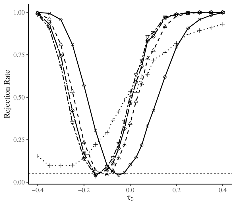
(a) constant $\pi_{0}$, $\mathrm{E}N_{z}=20$

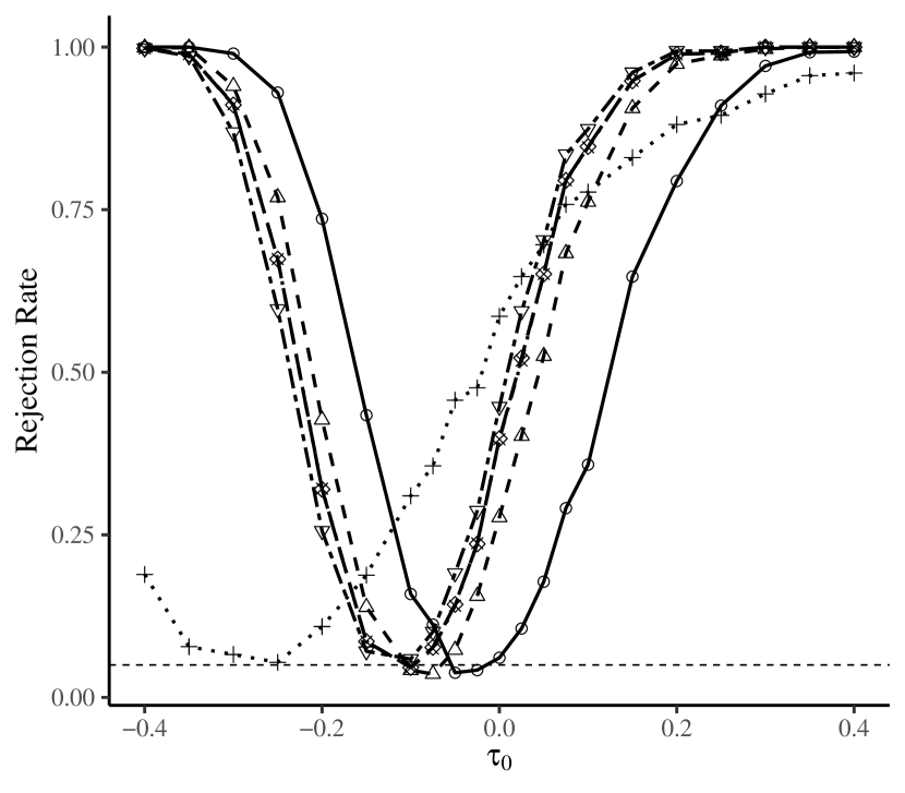
(b) constant $\pi_{0}$, $\mathrm{E}N_{z}=25$

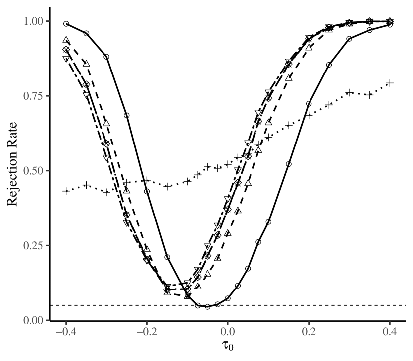
(c) heterogeneous $\pi_{0}$, $\mathrm{E}N_{z}=20$

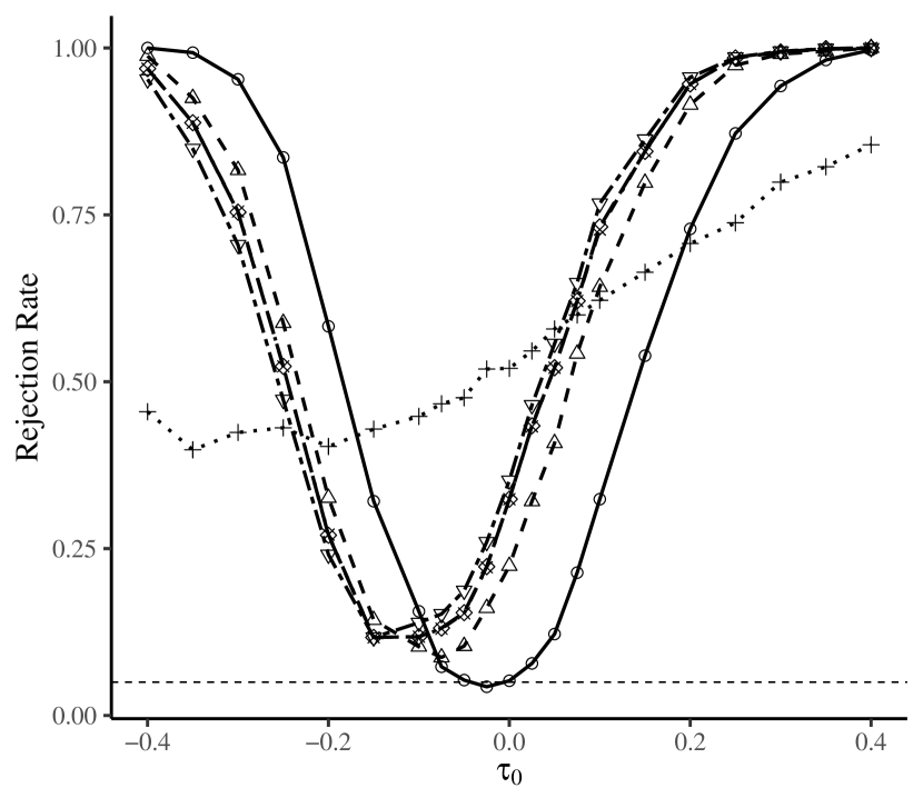
(d) heterogeneous $\pi_{0}$, $\mathrm{E}N_{z}=25$

Notes. Simulation results are based on 1000 replications using the DGP described in Section 4 with $K_{0}=2$. Panels (a) and (b) are with constant effects so that $\pi_{0}(X_{i})=\tau_{0}$. Panels (c) and (d) allow for covariate-dependent effects with $\pi_{0}(X_{i})=1-2X_{i}+\tau_{0}$. The power curves plot the rejection rate of testing $H_{0}:\tau_{0}=0$ at significance level $\alpha=0.05$. CIV denotes the categorical IV estimator with known $K_{0}$. “CIV ($K=2$)” and “CIV ($K=4$)” correspond to the proposed categorical IV estimators restricted to 2 and 4 support points in the first stage, “Lasso-IV (plug-in)” denotes IV estimator that uses lasso to estimate the optimal instrument using penalty parameters chosen via the plug-in rule of Belloni et al., (2012) , “Ridge-IV (cv)” denotes an IV estimator that uses ridge regression to estimate the optimal instrument using a penalty parameter chosen via 10-fold cross validation, and “xgboost-IV” and “ranger-IV” denote IV estimators that use gradient tree boosting as implemented by the xgboost package and random forests as implemented by the ranger package to estimate the optimal instrument, respectively.

References

- Aizer and Doyle Jr, (2015) Aizer, A. and Doyle Jr, J. J. (2015). Juvenile incarceration, human capital, and future crime: Evidence from randomly assigned judges. Quarterly Journal of Economics, 130(2):759–803.
- Amemiya, (1974) Amemiya, T. (1974). Multivariate regression and simultaneous equation models when the dependent variables are truncated normal. Econometrica, pages 999–1012.
- Angrist and Frandsen, (2022) Angrist, J. D. and Frandsen, B. (2022). Machine labor. Journal of Labor Economics, 40(S1):S97–S140.
- Angrist et al., (1999) Angrist, J. D., Imbens, G. W., and Krueger, A. B. (1999). Jackknife instrumental variables estimation. Journal of Applied Econometrics, 14(1):57–67.
- Angrist and Krueger, (1991) Angrist, J. D. and Krueger, A. B. (1991). Does compulsory school attendance affect schooling and earnings? Quarterly Journal of Economics, 106(4):979–1014.
- Angrist and Krueger, (1995) Angrist, J. D. and Krueger, A. B. (1995). Split-sample instrumental variables estimates of the return to schooling. Journal of Business & Economic Statistics, 13(2):225–235.
- Bekker, (1994) Bekker, P. A. (1994). Alternative approximations to the distributions of instrumental variable estimators. Econometrica: Journal of the Econometric Society, pages 657–681.
- Bekker and Van der Ploeg, (2005) Bekker, P. A. and Van der Ploeg, J. (2005). Instrumental variable estimation based on grouped data. Statistica Neerlandica, 59(3):239–267.
- Belloni et al., (2012) Belloni, A., Chen, D., Chernozhukov, V., and Hansen, C. (2012). Sparse models and methods for optimal instruments with an application to eminent domain. Econometrica, 80(6):2369–2429.
- Bester and Hansen, (2016) Bester, C. A. and Hansen, C. B. (2016). Grouped effects estimators in fixed effects models. Journal of Econometrics, 190(1):197–208.
- Bhuller et al., (2020) Bhuller, M., Dahl, G. B., Løken, K. V., and Mogstad, M. (2020). Incarceration, recidivism, and employment. Journal of Political Economy, 128(4):1269–1324.
- Blandhol et al., (2022) Blandhol, C., Bonney, J., Mogstad, M., and Torgovitsky, A. (2022). When is TSLS actually LATE? BFI Working Paper, (2022-16).
- Bonhomme and Manresa, (2015) Bonhomme, S. and Manresa, E. (2015). Grouped patterns of heterogeneity in panel data. Econometrica, 83(3):1147–1184.
- Bound et al., (1995) Bound, J., Jaeger, D. A., and Baker, R. M. (1995). Problems with instrumental variables estimation when the correlation between the instruments and the endogenous explanatory variable is weak. Journal of the American Statistical Association, 90(430):443–450.
- Carrasco, (2012) Carrasco, M. (2012). A regularization approach to the many instruments problem. Journal of Econometrics, 170(2):383–398.
- Chamberlain, (1987) Chamberlain, G. (1987). Asymptotic efficiency in estimation with conditional moment restrictions. Journal of Econometrics, 34(3):305–334.
- Chamberlain and Imbens, (2004) Chamberlain, G. and Imbens, G. (2004). Random effects estimators with many instrumental variables. Econometrica, 72(1):295–306.
- Chao and Swanson, (2005) Chao, J. C. and Swanson, N. R. (2005). Consistent estimation with a large number of weak instruments. Econometrica, 73(5):1673–1692.
- Chernozhukov et al., (2018) Chernozhukov, V., Chetverikov, D., Demirer, M., Duflo, E., Hansen, C., Newey, W., and Robins, J. (2018). Double/debiased machine learning for treatment and structural parameters: Double/debiased machine learning. The Econometrics Journal, 21(1).
- Chetverikov and Manresa, (2022) Chetverikov, D. and Manresa, E. (2022). Spectral and post-spectral estimators for grouped panel data models. arXiv preprint arXiv:2212.13324.
- Dhar et al., (2022) Dhar, D., Jain, T., and Jayachandran, S. (2022). Reshaping adolescents’ gender attitudes: Evidence from a school-based experiment in india. American Economic Review, 112(3):899–927.
- Donald and Newey, (2001) Donald, S. G. and Newey, W. K. (2001). Choosing the number of instruments. Econometrica, 69(5):1161–1191.
- Gilchrist and Sands, (2016) Gilchrist, D. S. and Sands, E. G. (2016). Something to talk about: Social spillovers in movie consumption. Journal of Political Economy, 124(5):1339–1382.
- Hahn and Moon, (2010) Hahn, J. and Moon, H. R. (2010). Panel data models with finite number of multiple equilibria. Econometric Theory, 26(3):863–881.
- Hansen et al., (2008) Hansen, C., Hausman, J., and Newey, W. (2008). Estimation with many instrumental variables. Journal of Business & Economic Statistics, 26(4):398–422.
- Hausman et al., (2012) Hausman, J. A., Newey, W. K., Woutersen, T., Chao, J. C., and Swanson, N. R. (2012). Instrumental variable estimation with heteroskedasticity and many instruments. Quantitative Economics, 3(2):211–255.
- Imbens and Angrist, (1994) Imbens, G. and Angrist, J. D. (1994). Identification and estimation of local average treatment effects. Econometrica, pages 467–475.
- Kling, (2006) Kling, J. R. (2006). Incarceration length, employment, and earnings. American Economic Review, 96(3):863–876.
- Kolesár, (2013) Kolesár, M. (2013). Estimation in an instrumental variables model with treatment effect heterogeneity. Working paper.
- Maestas et al., (2013) Maestas, N., Mullen, K. J., and Strand, A. (2013). Does disability insurance receipt discourage work? using examiner assignment to estimate causal effects of ssdi receipt. American economic review, 103(5):1797–1829.
- Mikusheva and Sun, (2022) Mikusheva, A. and Sun, L. (2022). Inference with many weak instruments. Review of Economic Studies, 89(5):2663–2686.
- Mugnier, (2022) Mugnier, M. (2022). Make the difference! computationally trivial estimators for grouped fixed effects models. arXiv preprint arXiv:2203.08879.
- Newey, (1990) Newey, W. K. (1990). Efficient instrumental variables estimation of nonlinear models. Econometrica, pages 809–837.
- Okui, (2011) Okui, R. (2011). Instrumental variable estimation in the presence of many moment conditions. Journal of Econometrics, 165(1):70–86.
- Su et al., (2016) Su, L., Shi, Z., and Phillips, P. C. (2016). Identifying latent structures in panel data. Econometrica, 84(6):2215–2264.
- Wang and Song, (2011) Wang, H. and Song, M. (2011). Ckmeans.1d.dp: optimal k-means clustering in one dimension by dynamic programming. The R journal, 3(2):29.
- Wüthrich and Zhu, (2021) Wüthrich, K. and Zhu, Y. (2021). Omitted variable bias of lasso-based inference methods: A finite sample analysis. Review of Economics and Statistics, pages 1–47.