Pricing and hedging for a sticky diffusion

Abstract

We consider a financial market model featuring a risky asset with a sticky geometric Brownian motion price dynamic and a constant interest rate $r\in\mathbb{R}$. We prove that the model is arbitrage-free if and only if $r=0$. In this case, we find the unique riskless replication strategy, derive the associated pricing equation. We also identify a class of replicable payoffs that coincides with the replicable payoffs in the standard Black-Scholes model. Last, we numerically evaluate discrete-time hedging and the hedging error incurred from misrepresenting price stickiness.

keywords and phrases: sticky diffusion, no-arbitrage condition, option pricing, risk-neutral valuation, riskless replication, hedging time-granularity

MSC 2020: Primary 91G20, 91G30; Secondary 60J60

1 Introduction

The seminal work of Black and Scholes [7] stands as the founding result in the theory of derivatives valuation. It also forms the basis of most pricing models in mathematical finance. This model proposes a riskless replication (or hedging) strategy of the payoff of a European contingent claim through a self-financing portfolio composed of the risky underlying asset(s) and the riskless asset. The claim’s price is the cost of the replication strategy. This allows effective market risk exposure management and equitable pricing of these financial products.

In this paper, we consider a variant of the Black-Scholes model where the price-dynamic $S$ of the risky asset is a sticky geometric Brownian motion. The process $S$ is a diffusion that behaves like a geometric Brownian motion away for certain price threshold(s), where it spends a positive amount time upon contact. We refer to this model as the sticky Black-Scholes model.

We establish that absence of arbitrage (NA) holds in the model if and only if $r=0$. In this case, we find the unique riskless replication strategy, derive the associated pricing equation and prove that, in this model, one can consider all payoff functions that are replicable for the standard Black-Scholes model. Last, we conduct numerical evaluations of discrete-time hedging and analyze the hedging error incurred when ignoring or misrepresenting price stickiness (model mismatch) as realized volatility or local volatility in a smooth model. Notably, this model aligns with observed price dynamics during a corporate takeover (see [5]).

First discovered by Feller [16], a sticky diffusion is a Markov process with continuous sample paths that spends a positive amount of time at some threshold(s). It is characterized by atom(s) in its speed measure [8] and can be expressed as time-delays of a non-sticky diffusion [1, 15, 23]. The time-delay is proportional to the local time of the diffusion at the sticky threshold.

In finance, sticky diffusions have been used to model short rates near zero [19, 25] and winning streak dynamics [17]. For other applications, see [9, 11, 12, 24, 26].

Outline:

In Section 2, we define the sticky Black-Scholes model. In Section 3 we recall some fundamental results related to arbitrage and risk-neutral valuation. In Section 4, we show that the sticky Black-Scholes model is arbitrage-free if and only if $r=0$. In Section 5, we derive the unique riskless replication strategy, the resulting pricing equation and identify a class of replicable payoffs. In section 6, we numerically evaluate properties of discrete-time hedging and the impact of model mismatch.

2 The Model

The Black-Scholes model makes the following assumptions:

1. infinite liquidity, divisibility of assets, and borrowing/lending capacity,

2. frictionless market (no transaction costs, no borrowing or lending rate),

3. possibility of continuous-time trading,

4. constant interest rate $r$,

5. geometric Brownian motion price dynamics.

The sticky Black-Scholes model consists in replacing (v) with ”the price process of the risky asset $S$ is a sticky geometric Brownian motion.” Thus, the prices of the risky and non-risky assets $(S,S^{0})$ solve the system the system (see [23]):

$$\frac{\,\mathrm{d}S_{t}}{S_{t}} =\mathbbm{1}_{S_{t}\neq\zeta}\left(\mu\,\mathrm{d}t+\sigma\,\mathrm{d}B_{t}\right),$$ (1)

$$\mathbbm{1}_{S_{t}=\zeta}\,\mathrm{d}t =\frac{\rho}{2}\,\mathrm{d}L^{\zeta}_{t}(S),$$

$$\frac{\,\mathrm{d}S^{0}_{t}}{S^{0}_{t}} =r\,\mathrm{d}t,$$

where $\mu,r\in\mathbb{R}$, $\sigma,\rho,\zeta>0$, and $B$ is a standard Brownian motion.

The process $S$ is a semimartingale with the explicit Doob-Meyer decomposition:

$$S_{t}=\mu\int_{0}^{t}S_{s}\mathbbm{1}_{S_{s}\neq\zeta}\,\mathrm{d}s+\sigma\int_{0}^{t}S_{s}\mathbbm{1}_{S_{s}\neq\zeta}\,\mathrm{d}B_{s}.$$ (2)

The process $S$ is the diffusion on $\operatorname{\mathbb{R}}_{+}$ defined through $s$ and $m$ (see [8, Chapter II] or [20, Chapter VII, §3]) where $s,m$ are defined for all $x>0$ by

$$s^{\prime}(x) =e^{-\frac{2\mu}{\sigma^{2}}\int^{x}\frac{1}{\zeta}\,\mathrm{d}\zeta}, m(\mathrm{d}x) =\frac{1}{s^{\prime}(x)}\frac{2}{\sigma^{2}x^{2}}\,\mathrm{d}x+\frac{\rho}{s^{\prime}(\zeta)}\delta_{\zeta}(\mathrm{d}x).$$ (3)

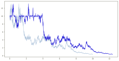
Figure 1: (left):  simulated sample path of the $(\mu=0,\sigma=0.25,\rho=1,\zeta=10)$ sticky (dark blue) and the $(\mu=0,\sigma=0.25)$ non-sticky (light blue) geometric Brownian motion. (right):  empiric density of the sticky (cyan) and transition density of the non-sticky (red) geometric Brownian motion. Sampling was done with the STMCA moment-matching random walk [4]

The process $S$ has an alternative path-wise representation akin to that of the geometric Brownian motion. Indeed, from the Itô lemma [3, Lemma 4.5], the process $(X,X^{0})=(\log S,\log S^{0})$ solves:

$$\,\mathrm{d}X_{t} =\left(\mu-\frac{\sigma^{2}}{2}\right)\mathbbm{1}_{X_{t}\neq\log\zeta}\,\mathrm{d}t+\sigma\mathbbm{1}_{X_{t}\neq\log\zeta}\,\mathrm{d}B_{t},$$ (4)

$$\mathbbm{1}_{X_{t}=\log\zeta}\,\mathrm{d}t =\frac{\rho}{2\zeta}\,\mathrm{d}L^{\log\zeta}_{t}(X),$$

$$\,\mathrm{d}X_{t}^{0} =r\,\mathrm{d}t.$$

Consequently, we derive the following expressions for the price dynamics:

$$S_{t} =S_{0}\exp\left(\left(\mu-\frac{\sigma^{2}}{2}\right)\int_{0}^{t}\mathbbm{1}_{S_{t}\neq\zeta}\,\mathrm{d}t+\sigma\int_{0}^{t}\mathbbm{1}_{S_{t}\neq\zeta}\,\mathrm{d}B_{t}\right),$$ (5)

$$\mathbbm{1}_{S_{t}=\zeta}\,\mathrm{d}t =\frac{\rho}{2}\,\mathrm{d}L^{\zeta}_{t}(S),$$

$$S^{0}_{t} =S^{0}_{0}\exp\left(rt\right).$$

Remark 2.1.

If $\rho=0$, then $S$ is a geometric Brownian motion. Indeed, in this case, $(s,m)$ defined in (3) are the scale function and speed measure of the geometric Brownian motion (see [8, p.132]). This can also be seen from (1), where if $\rho=0$, the process $S$ has a geometric Brownian dynamic away from $\zeta$ and spends almost surely no time at $\zeta$.

The process $(S,S^{0})$ is a $2$-dimensional sticky diffusion that, when $r\neq 0$, cannot be reduced to a time-change. The stickiness affecting the dynamic of the risky asset $S$ slows down its motion, while the log-value of the zero bond $\log(S^{0})$ steadily increases with rate $r$. This characteristic results in the violation the no-arbitrage hypothesis for the model when $r\not=0$.

3 Generic Results on Arbitrage and Valuation

This section presents fundamental results on arbitrage, payoff replication, and pricing.

Throughout the rest of the paper:

1. If $H$ is a predictable process and $S$ is a semi-martingale, the stochastic integral process is denoted by $(H\cdot S)$, expressed as:

   $$(H\cdot S)_{t}=\int_{0}^{t}H_{s}\,\mathrm{d}S_{s}.$$ (6)

2. If $\operatorname{Q},\operatorname{P}$ are two probability measures defined on the same measurable space $(\Omega,\operatorname{\mathcal{F}})$, $\operatorname{Q}\sim\operatorname{P}$ signifies their equivalence, i.e., $\operatorname{Q}\sim\operatorname{P}$ if and only if for all $A\in\operatorname{\mathcal{F}}$:

   $$\operatorname{P}(A)=0\quad\iff\quad\operatorname{Q}(A)=0.$$ (7)

3. For any probability measure $\operatorname{P}$, we denote with $\operatorname{E}^{\operatorname{P}}$ the expectation under $\operatorname{P}$.

The semi-martingale $S$ represents the price process of an asset traded in a market satisfying conditions (i)-(iii). We consider $S$ to be defined on a filtered probability space $(\Omega,(\operatorname{\mathcal{F}}_{t})_{t\geq 0},\operatorname{P})$ and adapted to $(\operatorname{\mathcal{F}}_{t})_{t\geq 0}$.

A trading strategy is a predictable process $\theta$ with respect to $(\operatorname{\mathcal{F}}_{t})_{t\geq 0}$, i.e., for all stopping times $\tau$, $\theta_{\tau}$ is $\operatorname{\mathcal{F}}_{\tau-}$-measurable.

An elementary trading strategy is a trading strategy of the form:

$$\theta_{t}=\sum_{i=0}^{n}\theta^{(i)}\mathbbm{1}_{t\in[\tau_{i},\tau_{i+1})}$$ (8)

with $n\in\operatorname{\mathbb{N}}$, $(\tau_{i})_{i\leq n}$ a family of Markovian stopping times, and $(\theta^{(i)})_{i}$ a family of random variables such that, for all $i$, $\theta^{(i)}$ is $\operatorname{\mathcal{F}}_{\tau_{i}}$-measurable.

An admissible trading strategy is an adapted predictable process $\theta$ with finite variation such that for some $M>0$ and all $t\geq 0$, $(\theta\cdot S)_{t}>-M$ almost surely.

Definition 3.1 (see [14], p.83-87).

The probability measure measure $\operatorname{Q}$ is called equivalent martingale measure if $\operatorname{Q}\sim\operatorname{P}$ and $S$ is a martingale on $(\Omega,(\operatorname{\mathcal{F}}_{t})_{t\geq 0},\operatorname{Q})$.

Definition 3.2 (arbitrage, Definition 2.1 of [18]).

An admissible strategy $\theta$ is an arbitrage opportunity on $[0,T]$ if $(\theta\cdot S)_{T}\geq 0$ almost surely and $\operatorname{P}\{(\theta\cdot S)_{T}>0\}>0$. A market is arbitrage-free (or satisfies (NA)) if, for any admissible $\theta$ with $(\theta\cdot S)_{T}\geq 0$ almost surely, the probability $\operatorname{P}\{(\theta\cdot S)_{T}>0\}=0$.

Theorem 3.3 (Theorem 6.5.1 of [14]).

Let $S$ be an $\operatorname{\mathbb{R}}^{d}$-valued semi-martingale defined on the probability space $(\Omega,(\operatorname{\mathcal{F}}_{t})_{t\geq 0},\operatorname{P})$. Then, $S$ satisfies (NA) iff there exists a probability measure $\operatorname{Q}\sim\operatorname{P}$ such that $S$ is a martingale on $(\Omega,(\operatorname{\mathcal{F}}_{t})_{t\geq 0},\operatorname{Q})$. We call $\operatorname{Q}$ a risk neutral measure.

The following result establishes a necessary condition for a semimartingale price model to be arbitrage-free. We will apply it to investigate absence of arbitrage in the sticky Black-Scholes model.

Theorem 3.4 (Theorem 3.5 of [13]).

Let $S$ be a d-dimensional, locally bounded semi-martingale $S$ that satisfies (NA). Then, the Doob-Meyer decomposition $S=M+A$ satisfies $\,\mathrm{d}A=\,\mathrm{d}\langle M\rangle h$, where h is a $d$-dimensional predictable process.

In absence of arbitrage and uniqueness of the equivalent martingale measure, the following result telegraphs the hedging mechanism of European contingent claims. It is also the result at the heart of the risk-neutral pricing framework. In this framework, the price at $t$ of a claim with a payoff of maturity $T>t$ is its expectancy under the risk-neutral probability $\operatorname{Q}$.

Theorem 3.5 (martingale representation theorem, Theorem 4.2.1 of [14]).

Let $W$ a standard Brownian motion defined of the probability space $(\Omega,(\operatorname{\mathcal{F}}_{t})_{t\geq 0},\operatorname{Q})$ with $(\operatorname{\mathcal{F}}_{t})_{t\geq 0}$ the natural filtration generated by $W$. We consider that $\operatorname{Q}$ is the unique equivalent martingale probability measure for $W$. Then, for all $f\in L^{1}(\Omega,\operatorname{\mathcal{F}}_{T},\operatorname{Q})$ there is a unique predictable process $\theta$ such that

$$f=\operatorname{E}^{\operatorname{Q}}(f)+\int_{0}^{T}\theta_{s}\,\mathrm{d}W_{s}$$ (9)

and for all $0\leq t\leq T$,

$$\operatorname{E}^{\operatorname{Q}}(f|\operatorname{\mathcal{F}}_{t})=\operatorname{E}^{\operatorname{Q}}(f)+\int_{0}^{t}\theta_{s}\,\mathrm{d}W_{s}$$ (10)

which implies that $(\theta\cdot W)$ is a uniformly integrable martingale.

Example 3.6.

We suppose the Black-Scholes model for a risky asset $S$ with risk-neutral measure $\operatorname{Q}$ and for simplicity and with $r=0$, where $S$ solves the SDE

$$\,\mathrm{d}S_{t}=\sigma S_{t}\,\mathrm{d}\widetilde{B}_{t},$$ (11)

with $\sigma>0$ and $\widetilde{B}$ being a $\operatorname{Q}$-Brownian motion. We consider a European contingent claim with maturity $T>0$ and terminal payoff $h(S_{T})\in L^{1}(\Omega,\operatorname{\mathcal{F}}_{T},\operatorname{Q})$. The filtration $(\operatorname{\mathcal{F}}_{t})_{t\geq 0}$ is generated by the driving Brownian motion. According to Theorem 3.5, there exists a unique predictable process $\theta$,

$$h(S_{T})=\operatorname{E}^{\operatorname{Q}}(h(S_{T}))+\int_{0}^{T}\theta_{s}\,\mathrm{d}\widetilde{B}_{s}=\operatorname{E}^{\operatorname{Q}}(h(S_{T}))+\int_{0}^{T}\theta_{s}\,\mathrm{d}S_{s},$$ (12)

where for all $t\leq T$, $\delta_{t}:=\theta_{t}/(\sigma_{t}S_{t})$. From [7], $\delta_{t}=v_{x}(t,S_{t})$, where $v(t,x)=\operatorname{E}^{\operatorname{Q}}(S_{T}|S_{t}=x)$. It is thus possible to replicate the payoff $h(S_{T})$ with a self-financing portfolio containing at $t$, $v_{x}(t,S_{t})$ parts of $S_{t}$.

Remark 3.7.

In the context of Example 3.6, European Call and Put contingent claims can be considered. This is evident as $S$ is a positive martingale in $L^{1}(\Omega,\operatorname{\mathcal{F}}_{T},\operatorname{Q})$, leading to the inequalities

$$\operatorname{E}^{\operatorname{Q}}\big{[}(S_{T}-K)+\big{]} \leq\operatorname{E}^{\operatorname{Q}}(S_{T})=S_{0}<\infty,$$

$$\operatorname{E}^{\operatorname{Q}}\big{[}(K-S_{T})+\big{]} \leq K<\infty.$$

Thus, $(S_{T}-K)_{+},(K-S_{T})_{+}\in L^{1}(\Omega,\operatorname{\mathcal{F}}_{T},\operatorname{Q})$.

4 Arbitrage

In this section we study arbitrage possibilities in the sticky Black-Scholes model. We first consider the case $r=0$, where we show that (NA) is verified by identifying the unique risk-neutral probability. We then establish that, when $r\neq 0$, the condition (NA) is not met. These provide sufficient and necessary conditions for the model to satisfy (NA).

Proposition 4.1.

Consider the sticky Black-Scholes model $(S,S^{0})$ as defined in Section 2 with $r=0$. The (NA) condition is verified and there is a unique risk-neutral probability $\operatorname{Q}$, defined via $\,\mathrm{d}\operatorname{Q}=\operatorname{\mathcal{E}}(\theta)_{T}\,\mathrm{d}\operatorname{P}$, where

$$\operatorname{\mathcal{E}}(\theta)_{t}=\exp\Big{(}\int_{0}^{t}\frac{\mu}{\sigma}\,\mathrm{d}B_{s}-\frac{1}{2}\int_{0}^{t}\Big{(}\frac{\mu}{\sigma}\Big{)}^{2}\,\mathrm{d}s\Big{)}.$$ (13)

Furthermore, $S$ solves

$$\,\mathrm{d}S_{t}/S_{t} =\sigma\mathbbm{1}_{S_{t}\neq\zeta}\,\mathrm{d}\widetilde{B}_{t},$$ (14)

$$\mathbbm{1}_{S_{t}=\zeta}\,\mathrm{d}t =\big{(}\rho/2\big{)}\,\mathrm{d}L^{\zeta}_{t}(S),$$

where $\widetilde{B}=(B_{t}-(\mu/\sigma)t)_{t\geq 0}$ is a $\operatorname{Q}$-standard Brownian motion.

Proof.

From the Girsanov theorem [3, Lemma 4.4], $S$ solves (14) under $\operatorname{Q}$.

The process $S$ is a local martingale since it is a stochastic integral with respect to a standard Brownian motion. Thus, from [20, Ch.IV, Corollary 1.25], to prove that $S$ is a martingale, it suffices to show that $\operatorname{E}^{\operatorname{Q}}(\langle S\rangle_{t})<\infty$.

From (5),

$$\operatorname{E}^{\operatorname{Q}}\big{(}\langle S\rangle_{t}\big{)}=\operatorname{E}^{\operatorname{Q}}\Big{(}\int_{0}^{t}\sigma^{2}S^{2}_{s}\mathbbm{1}_{S_{s}\not=\zeta}\,\mathrm{d}s\Big{)}\leq\sigma^{2}\int_{0}^{t}\operatorname{E}^{\operatorname{Q}}\big{(}S^{2}_{s}\big{)}\,\mathrm{d}s\\ =\sigma^{2}S^{2}_{0}\int_{0}^{t}\operatorname{E}^{\operatorname{Q}}\Big{(}\exp\Big{(}-\sigma^{2}\int_{0}^{s}\mathbbm{1}_{X_{u}\neq\zeta^{\prime}}\,\mathrm{d}u+2\sigma\int_{0}^{s}\mathbbm{1}_{X_{u}\neq\zeta^{\prime}}\,\mathrm{d}B_{u}\Big{)}\Big{)}\,\mathrm{d}s\leq S^{2}_{0}(e^{\sigma^{2}t}-1)$$ (15)

which for all $t\geq 0$, is finite. Thus, $S$ is a $Q$-martingale and, from Theorem 3.3, (NA) holds.

The uniqueness of the risk-neutral probability is guaranteed by [20, Chapter VIII, §1]. ∎

Theorem 4.2.

The sticky Black-Scholes model satisfies (NA) if and only if $r=0$.

Proof.

Let $\widetilde{S}:=S/S^{0}$. From (1) and the Itô lemma,

$$\,\mathrm{d}(e^{-rt}S_{t})=e^{-rt}\,\mathrm{d}S_{t}-re^{-rt}S_{t}\,\mathrm{d}t=\Big{(}\mu\mathbbm{1}_{S_{t}\not=\zeta}-r\Big{)}\widetilde{S}_{t}\,\mathrm{d}t+\sigma\mathbbm{1}_{S_{t}\not=\zeta}\widetilde{S}_{t}\,\mathrm{d}B_{t}.$$ (16)

Thus, $\widetilde{S}$ admits the following Doob-Meyer decomposition

$$\widetilde{S}_{t} =A_{t}+M_{t}, A_{t} :=S_{0}+\int_{0}^{t}\mu\widetilde{S}_{s}\mathbbm{1}_{S_{s}\not=\zeta}\,\mathrm{d}s-rt, M_{t} :=+\int_{0}^{t}\sigma\widetilde{S}_{s}\mathbbm{1}_{S_{s}\not=\zeta}\,\mathrm{d}B_{s},$$ (17)

where $A$ is a bounded variation process and $M$ is a local martingale. We observe that

$$\,\mathrm{d}A_{t} =-r\widetilde{S}_{t}\,\mathrm{d}t+\mu\widetilde{S}_{t}\mathbbm{1}_{S_{t}\not=\zeta}\,\mathrm{d}t, \,\mathrm{d}\langle M\rangle_{t} =\sigma^{2}\widetilde{S}^{2}_{t}\mathbbm{1}_{S_{t}\not=\zeta}\,\mathrm{d}t.$$ (18)

We note that the condition $\,\mathrm{d}A_{t}\ll\,\mathrm{d}\langle M\rangle_{t}$ holds if and only if $r=0$. From Theorem 3.4, this yields that if $r\neq 0$, (NA) is not satisfied. Conversely, when $r=0$, as established in Proposition 4.1, the (NA) condition is met. This completes the proof. ∎

Remark 4.3.

The issue that arises for the sticky Black-Scholes model when $r\neq 0$ is comparable to the one discussed in [22] for a diffusion with skew returns. There exists a local time term that cannot be offset by the quadratic variation of the martingale part $M$. Indeed, from (1) and (17), we have

$$A_{t}=\int_{0}^{t}(\mu\widetilde{S}_{s}-r)\mathbbm{1}_{S_{s}\not=\zeta}\,\mathrm{d}s-r\zeta\int_{0}^{t}\mathbbm{1}_{S_{s}=\zeta}\,\mathrm{d}s=\int_{0}^{t}(\mu\widetilde{S}_{s}-r)\mathbbm{1}_{S_{s}\not=\zeta}\,\mathrm{d}s-\frac{\rho r\zeta}{2}L^{\zeta}_{t}(S).$$ (19)

Remark 4.4.

We note that stickiness persists in the risk-neutral space. In particular, if the asset price $S$ is a sticky geometric Brownian motion, sticky at $\zeta>0$ with stickiness $\rho>0$, then, the risk-neutral dynamic (14) of $S$ is also a sticky geometric Brownian motion, sticky at $\zeta>0$ with stickiness $\rho>0$.

5 Pricing $\&$ hedging

We now derive the payoff replication strategy and the associated pricing equation in the context of the sticky Black-Scholes model.

These derivations are valid only in the case where $r=0$. When $r\neq 0$, the (NA) condition is not met and, as per Theorem 3.3, there is no equivalent probability measure for which discounted prices are martingales. In this case, Theorem 3.5 and the use of risk-neutral pricing techniques do not apply.

For the remainder of this section, we assume $r=0$. We consider the sticky Black-Scholes model defined in Section 2 with $r=0$, defined on the probability space $(\Omega,(\operatorname{\mathcal{F}}_{t})_{t\geq 0},\operatorname{P}_{x})$ so that $S_{0}=x$, $\operatorname{P}_{x}$-almost surely. Let $\operatorname{Q}_{x}$ be the equivalent martingale probability measure derived in Proposition 4.1.

Theorem 5.1 (pricing equation).

Let $V_{t}$ be the value at $t$ of a European contingent claim with terminal payoff $h(S_{T})$ so that $h(S_{T})\in L^{1}(\Omega,\operatorname{\mathcal{F}}_{T},\operatorname{Q}_{x})$. Then, $V_{t}=v(t,S_{t})$, where $v$ solves

$$\begin{dcases}v_{t}=-\frac{\sigma^{2}x^{2}}{2}v_{xx},&\forall(t,x)\in(0,T)\times(0,\infty),\\ \frac{\sigma^{2}\zeta^{2}}{2}v_{xx}(t,\zeta)=\frac{1}{\rho}\big{(}v_{x}(t,\zeta+)-v_{x}(t,\zeta-)\big{)},\\ v(T,x)=h(x).\end{dcases}$$ (20)

Proof.

From Theorem 3.3, there exists a probability measure $\operatorname{Q}_{x}$ under which the 2-dimensional process $(S/S^{0},S^{0}/S^{0})$ is a martingale. From Proposition 4.1, $\operatorname{Q}_{x}$ is unique and defined via

$$\mathrm{d}\operatorname{Q}_{x}/\mathrm{d}\operatorname{P}_{x}=\operatorname{\mathcal{E}}(\theta)_{t} :=\exp\Big{(}\int_{0}^{t}\theta_{s}B_{s}-\frac{1}{2}\int_{0}^{t}\theta^{2}_{s}\operatorname{d}\!{s}\Big{)}, \theta_{t} =\frac{\mu-r}{\sigma}.$$ (21)

The infinitesimal generator of $S$ under $\operatorname{Q}_{x}$ is defined for all $f\in\operatorname{dom}(\operatorname{L})$ by $\operatorname{L}f=((x\sigma)^{2}/2)f^{\prime\prime}$, where

$$\operatorname{dom}(\operatorname{L})=\Big{\{}f\in C_{b}^{0}(\operatorname{\mathbb{R}}_{+})\cap C^{2}(\operatorname{\mathbb{R}}_{+}\setminus\{\zeta\}):\frac{(\zeta\sigma)^{2}}{2}f^{\prime\prime}(\zeta)=(1/\rho)\big{(}f^{\prime}(\zeta+)-f^{\prime}(\zeta-)\big{)}\Big{\}},$$ (22)

$f^{\prime}$ is the right derivative of $f$ and $f^{\prime\prime}$ is the right-derivative of $f^{\prime}$.

For all $t\in[0,T]$ and $x>0$, let $v,u$ be the functions defined by

$$v(t,x) =\operatorname{E}^{\operatorname{Q}_{x}}(h(S_{T-t})), u(t,x) =v(T-t,x)=\operatorname{E}^{\operatorname{Q}_{x}}(h(S_{t})).$$ (23)

From Theorem 3.5, the price at $t$ of the European contingent claim of payoff $h$ and maturity $T$ is $v(t,S_{t})$.

We observe that $u(0,\cdot)=h$ and that $u$ solves the backward equation

$$\begin{dcases}u_{t}=\frac{\sigma^{2}x^{2}}{2}u_{xx},&\forall(t,x)\in(0,T)\times(0,\infty),\\ \frac{\sigma^{2}\zeta^{2}}{2}u_{xx}(t,\zeta)=\frac{1}{\rho}\big{(}u_{x}(t,\zeta+)-u_{x}(t,\zeta-)\big{)},\\ u(0,x)=h(x).\end{dcases}$$ (24)

This results in $v(t,x)=u(T-t,x)$ solving (20). This finishes the proof. ∎

Proposition 5.2 (replication strategy).

Let $v$ be the function defined in Theorem 5.1. The unique replication strategy $\delta$ for the payoff $h(S_{T})$ (refer to Theorem 3.5) is $\delta=(v_{x}(t,S_{t});\;t\in[0,T])$.

Proof.

Let $\operatorname{Q}$ be the unique probability measure for which $S$ is a martingale and $\widetilde{B}$ be the $\operatorname{Q}$-standard Brownian motion, defined in Proposition 4.1. Since $h(S_{T})\in L^{1}(\Omega,\operatorname{\mathcal{F}}_{T},\operatorname{Q}_{x})$, Theorem 3.5 guarantees a unique payoff replication strategy $\theta$ such that for all $t\leq T$,

$$\operatorname{E}^{\operatorname{Q}}(h(S_{T})|\operatorname{\mathcal{F}}_{t})=\operatorname{E}^{\operatorname{Q}}(h(S_{T}))+\int_{0}^{t}\theta_{s}\,\mathrm{d}\widetilde{B}_{s}.$$ (25)

In the standard Black-Scholes model, we could deduce from the replication strategy $\theta$ on the driving Brownian motion, a replication strategy $\delta$ on the price-process $S$ (see Example 3.6). We suppose we can do the same thing for $S$ sticky and that there exists a trading strategy $\delta$ such that for all $t\leq T$, $\theta_{t}\,\mathrm{d}\widetilde{B}_{t}=\delta_{t}\,\mathrm{d}S_{t}$.

Then, the value of the replication portfolio at all $t\leq T$ is

$$V_{t}:=v(t,S_{t})=\delta_{t}S_{t}+\delta^{0}_{t}S^{0}_{t}.$$ (26)

Let $\operatorname{L}$ be the infinitesimal generator of $S$ and $\operatorname{dom}(\operatorname{L})$ its domain, specified in (22). We observe that all $f\in\operatorname{dom}(\operatorname{L})$ are difference of convex functions. To elaborate, we define $\phi$ for all $x>0$ by

$$\phi(x)=f(x)-\frac{\rho(\zeta\sigma)^{2}}{2}f^{\prime\prime}(\zeta)(x-\zeta)_{+}.$$ (27)

Observing that $\phi\in C^{2}(\operatorname{\mathbb{R}}_{+})$, we can express $\phi$ as a sum of integrals based on the sign of $\phi^{\prime\prime}$. This structure implies that $\phi$ is a difference of two convex functions. Given that $x\rightarrow(x-\zeta)_{+}$ is convex, the function $f$ is also difference of convex functions.

From Theorem 5.1, for all $t<T$, $v(t,\cdot)\in\operatorname{dom}(\operatorname{L})$. From the Itô-Tanaka formula (see [20]),

$$\,\mathrm{d}V_{t}=\,\mathrm{d}v(t,S_{t})=v_{t}(t,S_{t})\,\mathrm{d}t+v_{x}(t,S_{t})\,\mathrm{d}S_{t}\\ +\frac{1}{2}v_{xx}(t,S_{t})\,\mathrm{d}\langle S\rangle_{t}+\frac{1}{2}\big{(}v_{x}(t,\zeta+)-v_{x}(t,\zeta-)\big{)}\,\mathrm{d}L^{\zeta}_{t}(S).$$ (28)

From (14),

$$\,\mathrm{d}\langle S\rangle_{t} =\sigma^{2}S^{2}_{t}\mathbbm{1}_{S_{t}\not=\zeta}\,\mathrm{d}t, \mathbbm{1}_{S_{t}=\zeta}\,\mathrm{d}t =\big{(}\rho/2\big{)}\,\mathrm{d}L^{\zeta}_{t}(S).$$ (29)

This combined with (20) yields

$$\frac{1}{2}\big{(}v_{x}(t,\zeta+)-v_{x}(t,\zeta-)\big{)}\,\mathrm{d}L^{\zeta}_{t}(S)=\frac{\rho\sigma^{2}\zeta^{2}}{4}u_{xx}(t,\zeta)\,\mathrm{d}L^{\zeta}_{t}(S)=-v_{t}(t,\zeta)\mathbbm{1}_{S_{t}=\zeta}\,\mathrm{d}t.$$ (30)

Consequently,

$$\,\mathrm{d}V_{t}=v_{t}(t,S_{t})\mathbbm{1}_{S_{t}\not=\zeta}\,\mathrm{d}t+v_{x}(t,S_{t})\,\mathrm{d}S_{t}+\frac{\sigma^{2}S^{2}_{t}}{2}v_{xx}(t,S_{t})\mathbbm{1}_{S_{t}\not=\zeta}\,\mathrm{d}t\\ +v_{t}(t,S_{t})\mathbbm{1}_{S_{t}=\zeta}\,\mathrm{d}t+\frac{1}{2}\big{(}v_{x}(t,\zeta+)-v_{x}(t,\zeta-)\big{)}\,\mathrm{d}L^{\zeta}_{t}(S)\\ =v_{x}(t,S_{t})\,\mathrm{d}S_{t}+\Big{(}v_{t}(t,S_{t})+\frac{\sigma^{2}S^{2}_{t}}{2}v_{xx}(t,S_{t})\Big{)}\mathbbm{1}_{S_{t}\not=\zeta}\,\mathrm{d}t.$$ (31)

From (26),(31) and since for all $t$, $S^{0}_{t}=1$,

$$\delta_{t}\,\mathrm{d}S_{t}=v_{x}(t,S_{t})\,\mathrm{d}S_{t}+\Big{(}v_{t}(t,S_{t})+\frac{\sigma^{2}S^{2}_{t}}{2}v_{xx}(t,S_{t})\Big{)}\mathbbm{1}_{S_{t}\not=\zeta}\,\mathrm{d}t.$$ (32)

Thus, the choice of hedging strategy $\delta_{t}=v_{x}(t,S_{t})$ results in the pricing PDE (20). This validates that for all $t\leq T$, $\theta_{t}\,\mathrm{d}\widetilde{B}_{t}=\delta_{t}\,\mathrm{d}S_{t}$ and finishes the proof. ∎

Remark 5.3.

The riskless replication strategy $\delta=(v_{x}(t,S_{t}))_{t}$ in the sticky Black-Scholes model is typically discontinuous at a sticky threshold. Indeed, from (24), if $v_{xx}(t,\zeta)\not=0$, then $v_{x}(t,\zeta+)-v_{x}(t,\zeta-)\not=0$.

For the rest of this section, for each $\rho\geq 0$, let $S^{(\rho)}$ be the solution of (1) and $\mathsf{H}_{\rho}$ be the class of replicable, in the sense of Theorem 3.5, payoff functions on $S^{(\rho)}$, given by

$$\mathsf{H}_{\rho}:=\big{\{}h\;\text{measurable}:\;h(S^{(\rho)}_{T})\in L^{1}(\Omega,\operatorname{\mathcal{F}}_{T},\operatorname{Q});\;\rho|h(\zeta)|<\infty\big{\}}.$$ (33)

We first prove that higher stickiness leads to lower prices for European derivative with convex payoffs. Then, we prove a result that justifies the usage of classical payoffs in the context of the sticky Black-Scholes model.

Lemma 5.4 (price monotonicity).

Let $\operatorname{Opt}[h](S^{(\rho)},x,T)$ be the price at $t=0$ of the contingent claim on the underlying asset $S^{(\rho)}$ with payoff function $h$, maturity $T>0$ and spot price $S^{(\rho)}_{0}=x$. If $h$ is convex, then

1. for all $x,T>0$, the application $[\rho\rightarrow\operatorname{Opt}[h](S^{(\rho)},x,T)]$ is decreasing,

2. for all $x>0$, $\rho\geq 0$, the application $[T\rightarrow\operatorname{Opt}[h](S^{(\rho)},x,T)]$ is increasing,

Proof.

Let $S^{(0)}$ be defined on the probability space $(\Omega,(\operatorname{\mathcal{F}}_{t})_{t\geq 0},\operatorname{P}_{x})$ such that $S^{(0)}=x$, $\operatorname{P}_{x}$-almost surely. Let $\operatorname{Q}_{x}$ be the risk neutral equivalent measure defined in Proposition 4.1. From Proposition 5.2,

$$\operatorname{Opt}[h](S^{(0)},x,T) =\operatorname{E}^{\operatorname{Q}_{x}}(h(S^{(0)}_{T})).$$ (34)

For all $\rho\geq 0$, let $\gamma_{\rho}$ be the random time change defined through its right-inverse $\gamma_{\rho}^{-1}(t)=t+(\rho/2)L^{\zeta}_{t}(S^{(0)})$. We observe that

1. if $\rho^{\prime}<\rho$, $0\leq\gamma_{\rho}(T)\leq\gamma_{\rho^{\prime}}(T)\leq T$,

2. from [21, p.278-279], $(S^{(0)}_{\gamma_{\rho}(t)})_{t\geq 0}=(S^{(\rho)}_{t})_{t\geq 0}$ in law,

3. $\gamma_{\rho}^{-1},\gamma_{\rho}$ are Markovian stopping times,

4. since $S^{(0)}$ is a $\operatorname{Q}_{x}$-martingale $(h(S^{(0)}_{t}))_{t\geq 0}$ is a $\operatorname{Q}_{x}$-submartingale.

Thus, from the stopping theorem, if $\rho^{\prime}<\rho$,

$$\operatorname{Opt}[h](S^{(\rho^{\prime})},x,T)=\operatorname{E}^{\operatorname{Q}}_{x}(h(S^{(\rho^{\prime})}_{T}))=\operatorname{E}^{\operatorname{Q}}_{x}(h(S^{(0)}_{\gamma_{\rho^{\prime}}(T)}))\\ \leq\operatorname{E}^{\operatorname{Q}}_{x}(h(S^{(0)}_{\gamma_{\rho}(T)}))=\operatorname{E}^{\operatorname{Q}}_{x}(h(S^{(\rho)}_{T}))=\operatorname{Opt}[h](S^{(\rho)},x,T).$$ (35)

With similar arguments, if $0\leq T\leq T^{\prime}$,

$$\operatorname{Opt}[h](S^{(\rho)},x,T)=\operatorname{E}^{\operatorname{Q}}_{x}(h(S^{(\rho)}_{T}))\leq\operatorname{E}^{\operatorname{Q}}_{x}(h(S^{(\rho)}_{T^{\prime}}))=\operatorname{Opt}[h](S^{(\rho)},x,T^{\prime}).$$ (36)

This finishes the proof. ∎

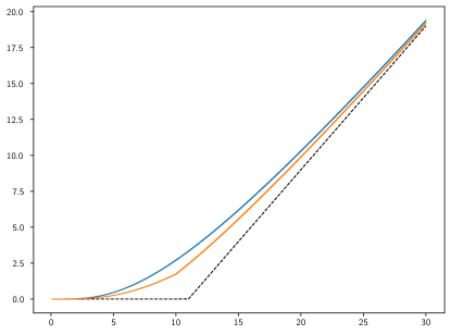
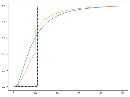
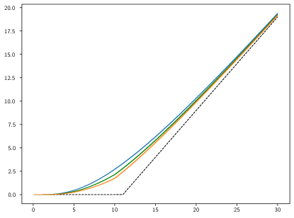
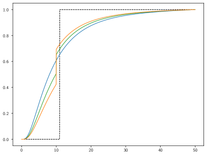
Figure 2: Price and delta of the Black-Scholes and sticky Black-Scholes. Finite-elements approximations of the price (left) and delta (right) curves of a Call option of strike $K=11$ and $T=10$ in the $(r,\sigma)=(0,0.25)$ standard Black-Scholes model (blue), the $(r,\sigma,\rho,\zeta)=(0,0.25,1.0,10.0)$ sticky Black-Scholes model (green) and the $(r,\sigma,\rho,\zeta)=(0,0.25,2.0,10.0)$ sticky Black-Scholes model (orange).

Proposition 5.5.

For all $0<\rho<\rho^{\prime}$, we have

$$\mathsf{H}_{0}\cap\{h\;\text{measurable}:\;|h(\zeta)|<\infty\}\subset\mathsf{H}_{\rho}\subset H_{\rho^{\prime}}.$$ (37)

Proof.

From Lemma 5.4, for all convex $h$, $\rho^{\prime}>\rho>0$ and $x>0$,

$$\operatorname{E}^{\operatorname{Q}_{x}}\big{(}h(S_{t}^{(\rho^{\prime})})\big{)}\leq\operatorname{E}^{\operatorname{Q}_{x}}\big{(}h(S_{t}^{(\rho)})\big{)}.$$ (38)

Thus, if $h$ is convex and in $H_{\rho}$, it is also in $H_{\rho^{\prime}}$. The second inclusion is then proven by considering differences of convex functions and smooth approximations of functions in $\mathsf{H}_{\rho}$.

For the first inclusion we repeat the same procedure by carefully excluding the case $|h(\zeta)|=\infty$. If $|h(\zeta)|=\infty$, since the occupation time of $\zeta$ by $S$ is positive with positive probability, we have that $\operatorname{E}^{\operatorname{Q}_{x}}\big{(}|h(S^{(\rho)}_{t})|\big{)}=\infty$. ∎

Remark 5.6.

Proposition 5.5 ensures that the $L^{1}$-condition of Theorem 3.5 on the payoff $h(S^{(\rho)}_{t})$ is met for all replicable payoff functions for the standard Black-Scholes model $\mathsf{H}_{0}$ such that $|h(\zeta)|<\infty$. In particular, from Remark 3.7, this holds for Call and Put payoffs.

6 Numerical experiments

This section is dedicated to numerical experiments aimed at evaluating practical aspects of hedging a contingent claim on an asset with a sticky price dynamic. We investigate two key properties. The first property involves the hedging time granularity of the sticky Black-Scholes model, referred to as “the impact on replication when the agent hedges in discrete time.” The second property is model mismatch, or “the impact on replication when an agent ignores or misrepresents price stickiness.”

In the rest of this section we consider the assets dynamic (1) with $r=0$, $\sigma=0.25$ and various degrees of stickiness $\rho\in\{0,1,2\}$ at the threshold $\zeta=10$. We recall that a stickiness value of $\rho=0$ corresponds to the standard Black-Scholes dynamic. The claim of interest will be a Call option with strike $K$ that delivers $(S_{T}-K)_{+}$ at maturity $T=10$.

Data: Stock price time-series $(S_{t})_{t\geq 0}$, Strike price $K$, Time to maturity $T$, Volatility $\sigma$, Stickiness $\rho$, Hedging window $\Delta t$

Result: Deltas and Portfolio Values over time

Compute/approximate the price function u_price$(x,K,T-t,\sigma,\rho)$;

Compute/approximate the delta function u_delta$(x,K,T-t,\sigma,\rho)$;

Initialize $cash$ to u_price$(S_{0},K,T,\sigma,\rho)$;

Initialize $t$ to $0$;

Initialize $initial\_delta$ to $0$;

while $t<T$ do

       Update time: $t\leftarrow t+\Delta t$;

       Calculate current option value: $price\leftarrow$ u_price$(S_{t},K,T-t,\sigma,\rho)$;

       Calculate current option delta: $delta\leftarrow$ u_delta$(S_{t},K,T-t,\sigma,\rho)$;

       Update cash: $cash\leftarrow cash-(delta-initial\_delta)\times S_{t}$;

       Update $initial\_delta$: $initial\_delta\leftarrow delta$;

       Update portfolio value: $portfolio\_value\leftarrow cash+(delta\times S_{t})-price$;

       Append $delta$ to the list of deltas;

       Append $portfolio\_value$ to the list of portfolio values;

      

return List of deltas, List of portfolio values;

Algorithm 1 Delta Hedging of an Option

6.1 Hedging time-granularity

The message of the Black-Scholes model is as follows: It is possible to replicate the payoff of a European option using a self-financing portfolio composed of quantities of the risky and non-risky assets. In particular, the option seller can hedge their risk by holding a portfolio that, at each time $t$, comprises $\delta_{t}=v_{x}(t,S_{t})$ parts of the risky asset.

However, a practical challenge arises since achieving this requires continuous rebalancing of the portfolio composition over time. This, as mentioned in [6], proves impossible in real-world scenarios as it necessitates an infinite number of operations. One way to address this is to introduce a hedging window $h>0$, resulting in hedging times $(t_{i})_{i}$ such that $t_{i+1}-t_{i}=h$. The agent can then rebalance the portfolio at each time $t_{i}$ so that for all $i$, they hold $v_{x}(t_{i},S_{t_{i}})$ parts of the risky asset on $[t_{i},t_{i+1})$. The resulting discretized version of the continuous-time hedging strategy $\delta$ is the strategy $\delta^{(N)}$ defined for all $t$ by

$$\delta^{(N)}_{t}=\delta_{[Nt]/N},$$ (39)

where $[x]=\sup\{k\in\operatorname{\mathbb{N}}:k\leq x\}$.

The PnLs at $t$ of the strategies $\delta$ and $\delta^{(N)}$ are

$$V_{t}(\delta)-V_{0}(\delta) =\int_{0}^{t}\delta_{s}\,\mathrm{d}S_{s}, V_{t}(\delta^{(N)})-V_{0}(\delta) =\int_{0}^{t}\delta^{(N)}_{s}\,\mathrm{d}S_{s},$$ (40)

where from Proposition 5.2, the option premium is $V_{0}(\delta)=\operatorname{E}^{\operatorname{Q}}\big{(}h(S_{T})\big{)}$ and $V_{t}(\delta)=\operatorname{E}^{\operatorname{Q}}\big{(}h(S_{T})|\operatorname{\mathcal{F}}_{t}\big{)}=\operatorname{E}^{\operatorname{Q}}_{S_{t}}\big{(}h(S_{T-t})\big{)}$.

This discrete replication strategy, outlined in Algorithm 1, results in replication errors known as the tracking error, defined by

$$\varepsilon^{(N)}_{t}:=V_{t}(\delta^{(N)})-V_{t}(\delta).$$ (41)

In [6], the metric used to assess the replication quality is the mean squared tracking error, defined by

$$\mathsf{R}_{T}^{(N)}:=\sqrt{\operatorname{E}^{\operatorname{Q}}\big{[}(\varepsilon^{(N)}_{T})^{2}\big{]}}.$$ (42)

Instead of this, we will quantify the replication properties of each model with the pair $\big{(}\operatorname{E}^{\operatorname{Q}}[\epsilon^{(N)}_{t}],\big{(}\operatorname{Var}^{\operatorname{Q}}[\epsilon^{(N)}_{t}]\big{)}^{1/2}\big{)}$, where $\operatorname{E}^{\operatorname{Q}}[\epsilon^{(N)}_{t}]$ is the expected replication PnL and $\big{(}\operatorname{Var}^{\operatorname{Q}}[\epsilon^{(N)}_{t}]\big{)}^{1/2}$ is the replication PnL standard deviation. The reason is that $\mathsf{R}_{t}^{(N)}$ is more adapted to the case where $\operatorname{E}^{\operatorname{Q}}\big{[}\varepsilon^{(N)}_{t}\big{]}=0$. If an agent is unsure about the pricing/replication model he applies, he is likely to miscalculate the option premium and end up with non-zero PnL, making the metric $\mathsf{R}_{t}^{(N)}$ irrelevant. This is the object of Section 6.2. Another reason for this choice is that the pair $\big{(}\operatorname{E}^{\operatorname{Q}}[\epsilon^{(N)}_{t}],\big{(}\operatorname{Var}^{\operatorname{Q}}[\epsilon^{(N)}_{t}]\big{)}^{1/2}\big{)}$ contains the information in $\mathsf{R}_{t}^{(N)}$. Indeed, the three quantities are linked with the relation:

$$\operatorname{Var}^{\operatorname{Q}}[\epsilon^{(N)}_{t}]=\big{(}\mathsf{R}_{t}^{(N)}\big{)}^{2}-\big{(}\operatorname{E}^{\operatorname{Q}}[\epsilon^{(N)}_{t}]\big{)}^{2}.$$ (43)

Stickiness $\rho=0$
N	premium	$\widehat{\mu}_{\operatorname*{MC}}$	$\widehat{\sigma}^{(N)}_{\operatorname*{MC}}$
2000	3.03923	-0.03438	0.06251
1000	3.03923	-0.03481	0.08605
250	3.03923	-0.03687	0.16781
100	3.03923	-0.04529	0.26832
10	3.03923	-0.00601	0.69078

Stickiness $\rho=1$
N	premium	$\widehat{\mu}_{\operatorname*{MC}}$	$\widehat{\sigma}^{(N)}_{\operatorname*{MC}}$
2000	2.43607	-0.02426	0.08783
1000	2.43607	-0.01573	0.17748
250	2.43607	-0.01959	0.29477
100	2.43607	-0.02013	0.40177
10	2.43607	-0.00182	0.80982

Stickiness $\rho=2$
N	premium	$\widehat{\mu}_{\operatorname*{MC}}$	$\widehat{\sigma}^{(N)}_{\operatorname*{MC}}$
2000	1.9976	-0.01487	0.04602
1000	1.9976	-0.01502	0.18474
250	1.9976	-0.03455	0.38181
100	1.9976	-0.03731	0.51832
10	1.9976	0.01637	0.96878

Table 1: Premiums and Monte Carlo estimation of the expected replication error (1000 simulated trajectories) for a Call $(K,T)=(10,10)$ for various stickiness and hedging windows. $N_{\operatorname*{MC}}=1000$.

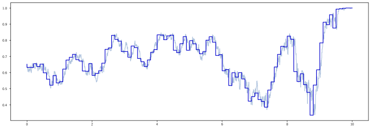
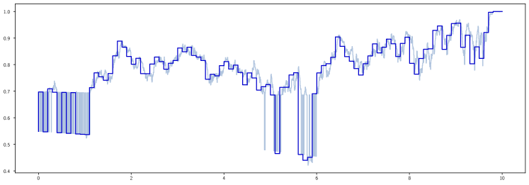
Figure 3: (top): Parts of risky asset in the payoff replication strategy for one sample path of $S$ with $\rho=0$, for (dark blue) $N=100$ and (light blue) $N=2000$. (bottom): Same, but with $\rho=1$.

We assess the discrete-time hedging error of the sticky Black-Scholes model as follows. We sample trajectories of the sticky geometric Brownian motion. Then, we apply Algorithm 1 to hedge a call option for various hedging windows. Last, we compute the empiric mean and standard deviation of the PnL with

$$\widehat{\mu}^{(N)}_{\operatorname*{MC}} =\frac{1}{N_{\operatorname*{MC}}}\sum_{i=1}^{N_{\operatorname*{MC}}}\varepsilon_{T}(\omega_{i}), \widehat{\sigma}^{(N)}_{\operatorname*{MC}} =\frac{1}{\sqrt{N_{\operatorname*{MC}}}}\sqrt{\sum_{i=1}^{N_{\operatorname*{MC}}}\big{(}\varepsilon_{T}(\omega_{i})-\widehat{\mu}_{\operatorname*{MC}}\big{)}^{2}}.$$ (44)

We do not have closed form expressions for the replication strategy and the induced prices for the sticky Black-Scholes model. We thus use finite differences approximations of the solution of (20). Simulation results are summarized in Table 1.

From numerical simulations, we observe the following:

1. Decrease in replication errors with higher hedging frequency $N$. Also, convergence seems to occur at the same rate as for the standard Black-Scholes model. In [6], it is proven that the rate of convergence for the Black-Scholes model is $\mathcal{O}(N^{-1/2})$.

2. Higher stickiness leads to higher tracking errors for coarse hedging time-windows. We attribute this behavior to the inherent discontinuity of the delta function at the sticky threshold. As depicted in Figure 2, higher stickiness at $\zeta$ corresponds to more substantial jumps in the delta, resulting in sudden shifts in portfolio composition whenever the price process $S$ crosses the sticky threshold. Consequently, the discrete-time hedging portfolio manifests substantial deviations in portfolio composition from the ideal configuration whenever the price crosses the sticky threshold. This is illustrated in Figure 3, where spikes and oscillations in the portfolio composition for fine-grained hedging do not appear in coarser regimes.

6.2 Model mismatch: constant volatility

Now, let’s assume that an agent intends to hedge a contingent claim on an underlying asset with a sticky geometric Brownian motion price dynamic with parameters $(\sigma,\rho,\zeta)$. The agent considers the following models:

Model 1:

The standard Black-Scholes model with volatility $\sigma$.

Model 2a:

The standard Black-Scholes model with volatility $\Sigma_{n}(X)$, where for some $T^{\prime}>0$, $\Sigma_{n}(X)$ is the estimator of the realized volatility on $[-T^{\prime},0)$ of the current sample path defined by

$$\Sigma_{n}(X)=\frac{1}{\sqrt{T^{\prime}}}\sqrt{\sum_{i=1}^{[nT^{\prime}]}\big{(}\log S_{-\frac{i}{n}}-\log S_{-\frac{i+1}{n}}\big{)}^{2}}.$$ (45)

Model 2b:

The standard Black-Scholes model with volatility $\Sigma_{n}(X)$, where $\Sigma_{n}(X)$ is the estimator of the realized volatility on $[0,T]$ of the current sample path defined by

$$\Sigma_{n}(X)=\frac{1}{\sqrt{T}}\sqrt{\sum_{i=1}^{n}\big{(}\log S_{\frac{i}{n}}-\log S_{\frac{i-1}{n}}\big{)}^{2}}.$$ (46)

Model 3:

The sticky Black-Scholes model with parameters $(\sigma,\rho,\zeta)$.

Model 1
$\rho$	prem.	fair p.	$\widehat{\mu}_{\operatorname*{MC}}$	$\widehat{\sigma}^{(N)}_{\operatorname*{MC}}$	adj.
0	3.073	3.0392	-0.0018	0.057	3.071
1	3.073	2.4360	0.6224	0.515	2.451
2	3.073	1.9976	1.0551	0.727	2.018

Model 2a
$\rho$	prem.	fair p.	$\widehat{\mu}_{\operatorname*{MC}}$	$\widehat{\sigma}^{(N)}_{\operatorname*{MC}}$	adj.
0	3.076	3.0392	0.0016	0.077	3.074
1	2.670	2.4360	0.2172	0.508	2.453
2	2.359	1.9976	0.3238	0.735	2.035

Model 2b
$\rho$	prem.	fair p.	$\widehat{\mu}_{\operatorname*{MC}}$	$\widehat{\sigma}^{(N)}_{\operatorname*{MC}}$	adj.
0	3.076	3.0392	-0.0004	0.032	3.076
1	2.670	2.4360	0.1420	0.166	2.528
2	2.356	1.9976	0.2207	0.197	2.135

Model 3
$\rho$	prem.	fair p.	$\widehat{\mu}_{\operatorname*{MC}}$	$\widehat{\sigma}^{(N)}_{\operatorname*{MC}}$	adj.
0	3.039	3.0392	-0.0343	0.062	3.073
1	2.436	2.4360	-0.0242	0.087	2.459
2	1.997	1.9976	-0.0014	0.046	1.998

Table 2: Theoretical premiums in each model, fair prices, mean PnLs and tracking errors for a Call $(K,T)=(10,10)$ on an assets with price-processes $\sigma=0.25$ sticky at $\zeta=10$ for various degrees of stickiness $\rho$ in each model. The hedging frequency is $N=2000$ and the number of simulated sample paths of each process is $N_{\operatorname*{MC}}=1000$.

According to Theorem 3.5, the fair price of the option with payoff $h$ at $T$ is $\operatorname{E}^{\operatorname{Q}}[h(S_{T})]$. From Proposition 5.1, this fair price is equivalent to the premium in Model 3, i.e.,

$$\text{Fair Price}=\big{(}\text{Premium in Model 3}\big{)}=\operatorname{E}^{\operatorname{Q}}[h(S_{T})].$$ (47)

Therefore, the premium is miscalculated in Models 1, 2a, and 2b. To address the premium miscalculation in each model, we introduce the following metric, which is the mean PnL corrected by the true premium:

$$\text{Adjusted}:=\text{Fair Price}-\widehat{\mu}_{\operatorname*{MC}}.$$ (48)

This adjustment compensates for the error made by the agent when using an incorrect model to compute premiums for contingent claims.

We observe the following:

1. Model 2b is unrealistic in practice as it necessitates a priori knowledge of future observations.

2. In Models 1 and 2a, the difference between the theoretical option premium and the expected replication PnL is approximately equivalent to the premium in Model 3. This is due to two facts. First, the agent ultimately holds $h(S_{T})$ at maturity. Second, given that the price dynamics are martingales on $(\Omega,(\operatorname{\mathcal{F}}_{t})_{t\geq 0},\operatorname{Q})$, from (9) the self-financing portfolio is also a martingale. Hence, the expected PnL of any self-financing portfolio is $0$ and the expected PnL of the option seller is

   $$\text{Premium}-\operatorname{E}^{\operatorname{Q}}[h(S_{T})],$$ (49)

   which equals $0$ only when pricing with the correct model, Model 3.

3. Among Models 1, 2a, and 3, it is Model 3 that exhibits the lowest hedging error, indicating superior replication properties (see Table 2).

6.3 Model mismatch: smooth SDE

We now suppose the agent misrepresents price stickiness as local volatility in a smooth SDE model.

It is possible to approximate in law diffusions with sticky features by smooth diffusions. We can define such an approximating sequence $Y^{n}$ as follows. For all $n$: let $Y^{n}$ solve $\,\mathrm{d}Y^{n}_{t}=\sigma_{n}(Y^{n}_{t})\,\mathrm{d}B^{n}_{t}$ with $B^{n}$ a standard Brownian motion and $\sigma_{n}$ smooth, such that

$$\frac{2}{\sigma_{n}^{2}(x)}\,\mathrm{d}x\xrightarrow[n\rightarrow\infty]{\text{weakly}}m(\mathrm{d}x):=\frac{2}{\sigma^{2}x^{2}}\,\mathrm{d}x+\rho\delta_{\zeta}(\mathrm{d}x),$$ (50)

where $m$ is the speed measure of $S$ for the risk-neutral probability $\operatorname{Q}$. Let also $v^{(n)}(t,x):=\operatorname{E}_{x}\big{(}h(Y^{n}_{T-t})\big{)}$ be the price curve for the model with diffusion coefficient $\sigma_{n}$. Since $\sigma_{n}$ is smooth, for all $t>0$, $x\rightarrow v^{(n)}(t,x)$ and $x\rightarrow v^{(n)}(t,x)$ are also smooth. From [10], $Y^{n}\longrightarrow X$ in law. This yields that, for all $x,t>0$,

$$\lim_{n\rightarrow\infty}v^{(n)}(t,x)=\operatorname{E}_{x}\big{(}h(X_{T-t})\big{)}.$$ (51)

Stickiness $\rho=0$
N	premium	$\widehat{\mu}_{\operatorname*{MC}}$	$\widehat{\sigma}^{(N)}_{\operatorname*{MC}}$
2000	3.03923	-0.03438	0.06251
1000	3.03923	-0.03481	0.08605
250	3.03923	-0.03687	0.16781
100	3.03923	-0.04529	0.26832
10	3.03923	-0.00601	0.69078

Stickiness $\rho=1$
N	premium	$\widehat{\mu}_{\operatorname*{MC}}$	$\widehat{\sigma}^{(N)}_{\operatorname*{MC}}$
2000	2.43607	-0.02311	0.17189
1000	2.43607	-0.01909	0.19802
250	2.43607	-0.02165	0.29681
100	2.43607	-0.02050	0.38760
10	2.43607	-0.01681	0.78004

Stickiness $\rho=2$
N	premium	$\widehat{\mu}_{\operatorname*{MC}}$	$\widehat{\sigma}^{(N)}_{\operatorname*{MC}}$
2000	1.9976	-0.00126	0.24402
1000	1.9976	-0.00939	0.28132
250	1.9976	-0.02760	0.40503
100	1.9976	-0.02075	0.52987
10	1.9976	0.00303	0.94837

Table 3: Same as Table 1 but for the locally linearly interpolated price curve around $\zeta$.

In Section 6.1, we approximated the delta function using an interpolation of the finite-difference scheme that preserved the discontinuity. We now use an approximation that does not preserve the discontinuity. Thus, the delta for the two approximations differ only locally around the threshold of stickiness. We observe, on numerical experiments, that the second method results in some irreductible hedging error (see Table 3). This indicates that it is not possible to hedge consistently a sticky diffusion using a smooth model. A hedging strategy, that is a smooth function of the spot price, cannot replicate the discontinuity of the true sticky hedging strategy (see Remark 5.3).

7 Conclusion

In conclusion, we proved that the sticky Black-Scholes model is consistent with the arbitrage-free pricing theory if and only if $r=0$. In that case we proved pricing and replication strategies. We proved that, in this model, we can replicate any Black-Scholes replicable payoff function. Numerical experiments indicate that the discrete-time hedging mean squared tracking error converges, at the rate $\mathcal{O}(N^{1/2})$, to $0$. This is the same rate as for the standard Black-Scholes model. We also observe that ignoring or misrepresenting stickiness leads to irreductible tracking errors. This highlights the importance to propose hedging strategies that properly take into account such features.

Acknowledgments

The author thanks Sara Mazzonetto and Denis Villemonais for insightful discussions and references on the subject.

References

- Amir [1991] Madjid Amir. Sticky Brownian motion as the strong limit of a sequence of random walks. Stochastic Process. Appl., 39(2):221–237, 1991.
- Anagnostakis [2022] Alexis Anagnostakis. Étude trajectorielle de diffusions singulières. PhD thesis, 2022. Thèse de doctorat dirigée par Lejay, Antoine et Villemonais, Denis Mathématiques Université de Lorraine 2022.
- Anagnostakis [2023] Alexis Anagnostakis. Functional convergence to the local time of a sticky diffusion. Electronic Journal of Probability, 28(88):1–26, 2023.
- Anagnostakis et al. [2023] Alexis Anagnostakis, Antoine Lejay, and Denis Villemonais. General diffusion processes as limit of time-space Markov chains. The Annals of Applied Probability, 33(5):3620 – 3651, 2023.
- Bass [2014] Richard F. Bass. A stochastic differential equation with a sticky point. Electron. J. Probab., 19:no. 32, 22, 2014.
- Bertsimas et al. [2001] Dimitris Bertsimas, Leonid Kogan, and Andrew W. Lo. When is time continuous? In Quantitative analysis in financial markets. Collected papers of the New York University Mathematical Finance Seminar. Vol. II, pages 71–102. Singapore: World Scientific, 2001.
- Black and Scholes [1973] Fischer Black and Myron Scholes. The pricing of options and corporate liabilities. Journal of Political Economy, 81(3):637–654, 1973.
- Borodin and Salminen [1996] Andrei N. Borodin and Paavo Salminen. Handbook of Brownian motion—facts and formulae. Probability and its Applications. Birkhäuser Verlag, Basel, 1996.
- Bou-Rabee and Holmes-Cerfon [2020] Nawaf Bou-Rabee and Miranda C. Holmes-Cerfon. Sticky Brownian motion and its numerical solution. SIAM Rev., 62(1):164–195, 2020.
- Brooks and Chacon [1982] J. K. Brooks and R. V. Chacon. Weak convergence of diffusions, their speed measures and time changes. Adv. Math., 46:200–216, 1982.
- Calsina and Farkas [2012] Àngel Calsina and József Z. Farkas. Steady states in a structured epidemic model with Wentzell boundary condition. J. Evol. Equ., 12(3):495–512, 2012.
- Davies and Truman [1994] M. J. Davies and A. Truman. Brownian motion with a sticky boundary and point sources in quantum mechanics. volume 20, pages 173–193. 1994. Lagrange geometry, Finsler spaces and noise applied in biology and physics.
- Delbaen and Schachermayer [1995] Freddy Delbaen and Walter Schachermayer. The existence of absolutely continuous local martingale measures. Ann. Appl. Probab., 5(4):926–945, 1995.
- Delbaen and Schachermayer [2006] Freddy Delbaen and Walter Schachermayer. The mathematics of arbitrage. Springer Finance. Berlin: Springer, 2006.
- Engelbert and Peskir [2014] Hans-Jürgen Engelbert and Goran Peskir. Stochastic differential equations for sticky Brownian motion. Stochastics, 86(6):993–1021, 2014.
- Feller [1952] Wiliam Feller. The parabolic differential equations and the associated semigroups of transformation. Ann. Math. (2), 55:468–519, 1952.
- Feng et al. [2020] Runhuan Feng, Pingping Jiang, and Hans Volkmer. Modeling financial market movement with winning streaks: Sticky maximum process. ERN: Asset Pricing Models (Topic), 2020.
- Guasoni [2006] Paolo Guasoni. No arbitrage under transaction costs, with fractional Brownian motion and beyond. Math. Finance, 16(3):569–582, 2006.
- Nie and Linetsky [2019] Yutian Nie and Vadim Linetsky. Sticky reflecting ornstein-uhlenbeck diffusions and the vasicek interest rate model with the sticky zero lower bound. Stochastic Models, 0(0):1–19, 2019.
- Revuz and Yor [1999] Daniel Revuz and Marc Yor. Continuous martingales and Brownian motion, volume 293 of Grundlehren der Mathematischen Wissenschaften [Fundamental Principles of Mathematical Sciences]. Springer-Verlag, Berlin, third edition, 1999.
- Rogers and Williams [2000] L. C. G. Rogers and David Williams. Diffusions, Markov processes, and martingales. Vol. 2. Cambridge Mathematical Library. Cambridge University Press, Cambridge, 2000. Itô calculus, Reprint of the second (1994) edition.
- Rossello [2012] Damiano Rossello. Arbitrage in skew Brownian motion models. Insur. Math. Econ., 50(1):50–56, 2012.
- Salins and Spiliopoulos [2017] Michael Salins and Konstantinos Spiliopoulos. Markov processes with spatial delay: path space characterization, occupation time and properties. Stoch. Dyn., 17(6):21, 2017. Id/No 1750042.
- Stell [1991] George Stell. Sticky spheres and related systems. Journal of Statistical Physics, 63:1203–1221, 1991.
- Zhang and Tian [2022] Haoyan Zhang and Yingxu Tian. Hitting time problems of sticky brownian motion and their applications in optimal stopping and bond pricing. Methodology and Computing in Applied Probability, 24, 06 2022.
- Zhu [2013] John Y. Zhu. Optimal contracts with shirking. Rev. Econ. Stud., 80(2):812–839, 2013.