Total Angular Momentum Conservation in Ehrenfest Dynamics with a Truncated Basis of Adiabatic States

Abstract

We show that standard Ehrenfest dynamics does not conserve linear and angular momentum when using a basis of truncated adiabatic states. However, we also show that previously proposed effective Ehrenfest equations of motionAmano and Takatsuka (2005); Krishna (2007) involving the non-Abelian Berry force do maintain momentum conservation. As a numerical example, we investigate the Kramers’ doublet of the methoxy radical using generalized Hartree-Fock with spin-orbit coupling and confirm angular momentum is conserved with the proper equations of motion. Our work makes clear some of the limitations of the Born-Oppenheimer approximation when using ab initio electronic structure theory to treat systems with unpaired electronic spin degrees of freedom and we demonstrate that Ehrenfest dynamics can offer much improved, qualitatively correct results.

I Introduction

Given the speed and power of modern computational supercomputers, nonadiabatic dynamics is widely used today to study ultrafast photochemical and charge-transfer dynamics (as probed by state-of-the-art experiments).Nelson et al. (2014) When connecting with experiments, however, in practice nonadiabatic simulations must almost always make a quantum-classical approximationTully (1998); Egorov, Rabani, and Berne (1999); Kapral and Ciccotti (1999); Curchod, Rothlisberger, and Tavernelli (2013); Römer and Burghardt (2013a); Crespo-Otero and Barbatti (2018) in order to be computationaly feasible. The fundamental assumption of propagating nuclei classically and the electrons quantum mechanically inevitably raises the issue of how to correctly incorporate the feedback between the quantum and the classical subsystems. One of the most popular choices at present is the surface hopping approach, Tully (1990); Barbatti (2011); Wang, Akimov, and Prezhdo (2016); Subotnik et al. (2016) whereby a swarm of trajectories move along a single adiabatic surface, and stochastically hop between surfaces to account for nonadiabatic effects. As we have documented recently,Wu et al. (2022) the surface-hopping algorithm faces difficulties in the presence of spin-orbit coupling (SOC), which we will address in a separate paper. A second approach, orthogonal to the surface-hopping ansatz, is to include the interaction between the quantum and classical subsystems in a mean-field way, which gives rise to the standard Ehrenfest approachMicha (1983); Billing (1983); Sawada, Nitzan, and Metiu (1985); Li et al. (2005)–an approach which is always well-defined (with or without SOC).

The pros and cons of Ehrenfest dynamics are well-known within the community.Meyer and Miller (1979); Andrew et al. (2004); Parandekar and Tully (2005, 2006); Curchod and Martínez (2018); Esch and Levine (2020, 2021); Shu and Truhlar (2023) Ehrenfest is most advantageous if there are frequent transitions between nearly parallel states, and one can work with either a handful or a dense manifoldFedorov and Levine (2019) of such states. However, the mean-field approximation between the quantum and classical subsystems can break down when there is a strong coupling between the two subsystems (e.g. when two potential energy surfaces are very displaced from each other); in such a case, methods such as multi-configurational Ehrenfest have been developed.Shalashilin (2009); Römer and Burghardt (2013b) Standard Ehrenfest also cannot account for decoherence nor achieve detailed balance,Parandekar and Tully (2005, 2006) which are important when studying systems in the condensed phase; various correction schemes have been proposed to address these deficiencies as wellZhu et al. (2004); Zhu, Jasper, and Truhlar (2004); Akimov, Long, and Prezhdo (2014); Esch and Levine (2020, 2021); Shu and Truhlar (2023). As a sidenote, we mention that, in this paper, we will concern ourselves strictly with what is known as “linear-response” Ehrenfest, where the electronic wavefunction is expanded in a basis of adiabatic/diabatic states; we will not concern ourselves with real-time Ehrenfest dynamics,Li et al. (2005); Isborn, Li, and Tully (2007) whereby the electronic wavefunction is propagated directly in the original atomic orbital basis.

Now, as a practical matter, there are several means by which one can judge the value of any dynamical approach. Almost always, the very first constraint on any good dynamics algorithm is energy conservation; in fact, checking for energy conservation is usually the very first means of making sure one’s code is free of bugs. Beyond energy conservation, in the absence of an external torque on the system, a second constraint is that the total angular momentum is also conserved. Interestingly, as opposed to energy conservation, angular momentum conservation is rarely emphasized in the context of nonadiabatic dynamics (though see below). Consider the most standard class of molecular dynamics, namely single-state dynamics within the Born-Oppenheimer (BO) approximation. For such dynamics, the electronic linear and angular momentum are usually neglected (or more formally folded into the nuclear degrees of freedom),Littlejohn, Rawlinson, and Subotnik (2023) and the nuclear linear and angular momentum are conserved due to translational symmetry and isotropy of space. However, as we recently showed,Bian et al. (2023) if one runs BO dynamics (without Berry force) along one of the degenerate doublet surfaces (in the presence of spin-orbit coupling) and keeps track of the fluctuating electronic angular momentum, one will inevitably compute a total angular momentum that fluctuates (i.e. one will predict a violation of angular momentum conservation).

Now, one means to resolve this paradox is not to use Born-Oppenheimer at all, but rather exact factorization,Abedi, Maitra, and Gross (2010, 2012); Vindel-Zandbergen, Matsika, and Maitra (2022) where angular momentum exchange was recently explored.Li, Requist, and Gross (2022) As pointed out in Ref. 36, however, an even simpler resolution to this paradox is that, within BO theory, one must include a Berry force (see below) acting on the nuclear motion. More precisely, for nonadiabatic systems with odd numbers of electrons plus SOC, the on-diagonal derivative coupling $\bm{d}$ is not zero, and so the nuclear kinetic momentum $\bm{\pi}_{\rm n}$ is not equivalent to the canonical momentum $\bm{P}_{\rm n}$ (recall that $\bm{\pi}_{\rm n}=\bm{P}_{\rm n}-i\hbar\bm{d}$). In order to minimize gauge problems, the usual approach is then to pick one adiabat from the Kramers’ pair to run along (say, $j$, which is computed from some approximate electronic structure technique) and then to propagate the nuclear kinetic momentum $\bm{\pi}_{\rm n}$; the latter step inevitably introduces the Abelian Berry force in the equation of motion for $\bm{\pi}_{\rm n}$, $\bm{F}^{{\rm Berry},I}_{j}=i\hbar(\nabla_{\rm n}\crossproduct\bm{d}_{jj})\cdot\frac{\bm{\pi}_{\rm n}}{M_{I}}$. As shown in Ref.36, including the pseudo-magnetic Berry force allows for a full exchange of angular momentum between electronic, nuclear, and spin degrees of freedom. Of course, there is still no guarantee that the dynamics are correct (i.e. following one adiabat of a pair), but at least the resulting dynamics are guaranteed to conserve the total angular momentum.

The background above raises crucial questions for the field of nonadiabatic dynamics. If one needs to go beyond BO dynamics, one can ask: do nonadiabatic dynamics algorithms conserve the total (electronic plus nuclear) momentum? In a recent paper, Shu et. alShu et al. (2020) have recently shown that the nuclear angular momentum is not conserved within an ab initio Ehrenfest scheme propagated in an adiabatic basis. In Ref. 41, the authors addressed this issue by projecting out the translational and rotational components of the derivative coupling that enters the force; see Eq. 18. While this scheme offers a practical way to conserve nuclear angular momentum, we will show below that the problems arising in Ref. 41 are at bottom created by using a truncated adiabatic basis, for which there is a rigorous (not ad hoc) solution. Deriving and understanding such a solution is the main focus of the present paper but in a nutshell, if BO dynamics require the Abelian Berry curvature in order to maintain momentum conservation, nonadiabatic Ehrenfest dynamics in a truncated basis require the non-Abelian Berry curvature Mead (1992) in order to achieve the same feat.

Finally, before concluding this section, a few words are appropriate regarding spin. The most obvious cases where we expect angular momentum conservation to be interesting, are systems with a flow of angular momentum between different degrees of freedom (including nuclear, electronic and spin degrees of freedom). For organic systems, the spin degree of freedom often operates on a much longer time scale than the electronic degree of freedom and sometimes even longer than the nuclear motion. In such cases, the validity of the BO approximation is dubious. Indeed, in this paper we will show that a simple rotation of the methoxy radical breaks the BO approximation because, within the BO approximation, the total spin vector rotates with the molecule instantaneously (which is incorrect). One would hope that the Ehrenfest equations of motion would perform far better, and indeed Ehrenfest does (correctly) slows down the spin change with the nuclear motion.

This paper is organized as follows. In Section II, we begin by demonstrating momentum conservation for Ehrenfest dynamics propagated over a complete electronic Hilbert space; this conclusion holds whether one performs the dynamics in a diabatic or adiabatic basis, and by comparing the calculations in the two different basis sets, one inevitably learns about the non-Abelian Berry curvature. In Sec. III, we then remove the assumption of a complete set of states and show that, according to standard Ehrenfest dynamics, neither linear and angular momentum are conserved in a truncated set of states. To restore momentum conservation in the presence of a truncated basis, we show that the equations of motion must include the non-Abelian Berry curvature and we present the relevant Hamiltonian from which Hamilton’s equations can be derived (where the final form agrees with the derivations in Refs. 1 and 2). In Sec. VI, in order to demonstrate the importance of momentum conservation, we perform two ab initio Ehrenfest calculations of the methoxy radical in the Kramers’ pair basis. We study both excitation of a vibration and excitation of angular momentum. These two cases make clear that including the non-Abelian Berry curvature can have a strong impact on the resulting spin dynamics and that, more generally, the BO approximation can badly break down in the presence of unpaired electrons. In Sec.VIII, we conclude and discuss future possible ab initio directions.

II Theory: Dynamics Within A Complete (Untruncated) Electronic Hilbert Space

We begin our analysis by assuming that we are working in a complete (untruncated) electronic vector space with zero curvature. This scenario represents a very ideal condition because the electronic Hilbert space is immense – requiring an enormous number (infinite) of one-particle electronic basis functions and then an even larger number (infinite) of many-body electronic wavefunctions (and just about any finite basis will exhibit a nonzero Berry curvatureMead (1992)). Nevertheless, the analysis below will still be useful insofar as teaching us how to understand how the Ehrenfest equations can take different form in different representations.

II.1 A Strictly Diabatic Representation

To begin our discussion, let us imagine that we are given an electronic Hamiltonian expressed in a strictly diabatic basis; in other words, the electronic basis does not depend at all on nuclear position. The Hamiltonian ($\tilde{\bm{H}}$) and the energy ($\tilde{E}$) are postulated to be of the form:

$$\tilde{\bm{H}} = \sum_{I}\frac{{\bm{P}}_{\rm n}^{I^{2}}}{2M_{I}}+\tilde{\bm{V}}$$ (1)

$$\tilde{E} = \sum_{I}\frac{{\bm{P}}_{\rm n}^{I^{2}}}{2M_{I}}+\mbox{Tr}\left(\tilde{\bm{\sigma}}\tilde{\bm{V}}\right)$$ (2)

where we denote the classical nuclear position $\bm{R}_{\rm n}$ and nuclear momentum $\bm{P}_{\rm n}$. Here and below we use the indices $IJ$ for nuclei and $\alpha\beta\gamma$ for the Cartesian indices $xyz$. The potential operator $\tilde{\bm{V}}=\tilde{\bm{T}}_{\rm e}+\tilde{\bm{V}}_{\rm ee}+\tilde{\bm{V}}_{\rm en}+\tilde{\bm{V}}_{\rm nn}$ includes the electronic kinetic energy, electron-electron interaction, and the electron-nuclear Coulomb interaction, and nuclear-nuclear repulsion term, respectively. We use the notation "~" to indicate operators in a diabatic basis. For the energy expression, the first term is the nuclear kinetic energy and the second term is the potential energy term that one computes by integrating over the electronic degree of freedom with the electronic density operator $\tilde{\bm{\sigma}}$ in a diabatic basis.

According to Hamilton’s equations, the equations of motions for nuclear position and momentum are:

$$\dot{R}^{I\alpha}_{\rm n} = \frac{\partial\tilde{E}}{\partial P^{I\alpha}_{\rm n}}=\frac{P^{I\alpha}_{\rm n}}{M_{I}}$$ (3)

$$\dot{P}^{I\alpha}_{\rm n} = -\frac{\partial\tilde{E}}{\partial R^{I\alpha}_{\rm n}}=-\mbox{Tr}\left(\tilde{\bm{\sigma}}\frac{\partial\tilde{\bm{V}}}{\partial R^{I\alpha}_{\rm n}}\right)$$ (4)

The associated density matrix operator evolves according to the Quantum Liouville equation,

$$\dot{\tilde{\bm{\sigma}}}=-\frac{i}{\hbar}\left[\tilde{\bm{V}},\tilde{\bm{\sigma}}\right]$$ (5)

Using Eqs. 3 and 4, it is straightforward to show that the total energy in diabatic representation (Eq. 2) is conserved $\frac{d\tilde{E}}{dt}=0$.

At this point, it will be helpful to define nuclear angular momentum:

$${J}^{\alpha}_{\rm n}\equiv\sum_{I\beta\gamma}\epsilon_{\alpha\beta\gamma}R^{I\beta}_{\rm n}M_{I}\dot{R}^{I\gamma}_{\rm n}$$ (6)

Here $\epsilon_{\alpha\beta\gamma}$ is the Levi-Civita symbol. Using Eq. 3 above, it follows that we can also write:

$${J}^{\alpha}_{\rm n}=\sum_{I\beta\gamma}\epsilon_{\alpha\beta\gamma}R^{I\beta}_{\rm n}P^{I\gamma}_{\rm n}$$ (7)

$$\dot{J}^{\alpha}_{\rm n}=\sum_{I\beta\gamma}\epsilon_{\alpha\beta\gamma}R^{I\beta}_{\rm n}\dot{P}^{I\gamma}_{\rm n}$$ (8)

With Eq.4 and Eq.5, we can now evaluate the time-derivative of the total linear and angular momentum

$$\dot{P}_{\rm tot}^{\alpha} = \dot{P}_{\rm n}^{\alpha}+\mbox{Tr}\left(\dot{\tilde{\bm{\sigma}}}{{\tilde{\bm{P}}}}_{\rm e}^{\alpha}\right)$$ (9)

$$= -\sum_{I}\mbox{Tr}\left(\tilde{\bm{\sigma}}\frac{\partial\tilde{\bm{V}}}{\partial R^{I\alpha}_{\rm n}}\right)-\frac{i}{\hbar}\mbox{Tr}\left(\tilde{\bm{\sigma}}[{{\tilde{\bm{P}}}}_{\rm e}^{\alpha},\tilde{\bm{V}}]\right)$$

$$\dot{J}_{\rm tot}^{\alpha} = \dot{J}_{\rm n}^{\alpha}+\mbox{Tr}\left(\dot{\tilde{\bm{\sigma}}}{{\tilde{\bm{J}}}}_{\rm e}^{\alpha}\right)$$ (10)

$$= \sum_{I\beta\gamma}\epsilon_{\alpha\beta\gamma}R^{I\beta}_{\rm n}\dot{P}^{I\gamma}_{\rm n}-\frac{i}{\hbar}\mbox{Tr}\left(\tilde{\bm{\sigma}}[{{\tilde{\bm{J}}}}_{\rm e}^{\alpha},\tilde{\bm{V}}]\right)$$

Finally, because we have assumed a complete electronic Hilbert space, for a finite system in real space, translational symmetry and the isotropy of space imply the following identities:

$$\Big{[}\tilde{\bm{P}}_{\rm n}+\tilde{\bm{P}}_{\rm e},\tilde{\bm{V}}\Big{]} = 0$$ (11)

$$\Big{[}\tilde{\bm{J}}_{\rm n}+\tilde{\bm{J}}_{\rm e},\tilde{\bm{V}}\Big{]} = 0$$ (12)

These equations lead to the following further identities:

$$-\frac{i}{\hbar}[{{\tilde{\bm{P}}}}_{\rm e}^{\alpha},\tilde{\bm{V}}] = \frac{i}{\hbar}[{{\tilde{\bm{P}}}}_{\rm n}^{\alpha},\tilde{\bm{V}}]=\frac{\partial\tilde{\bm{V}}}{\partial R^{\alpha}_{\rm n}}$$ (13)

$$-\frac{i}{\hbar}[{{\tilde{\bm{J}}}}_{\rm e}^{\alpha},\tilde{\bm{V}}] = \frac{i}{\hbar}[{{\tilde{\bm{J}}}}_{\rm n}^{\alpha},\tilde{\bm{V}}]=\sum_{I\beta\gamma}\epsilon_{\alpha\beta\gamma}R^{I\beta}_{\rm n}\frac{\partial\tilde{\bm{V}}}{\partial R^{I\gamma}_{\rm n}}$$ (14)

If we plug the commutators above into Eq. 9 and Eq.10, we find momentum conservation $\dot{P}_{\rm tot}^{\alpha}=\dot{J}_{\rm tot}^{\alpha}=0$.

II.2 Adiabatic Representation

The above equations of motion for Ehrenfest dynamics can be transformed into an adiabatic basis as well with the same conclusions, though we will find that the existence of a complete electronic basis is expressed differently than what we found in Eqs. 11-12. To proceed, let us define a unitary matrix that transforms the diabatic basis (with indices $abcd$) to adiabatic basis (with indices $ijkl$): $\ket{\psi_{k}}=\sum_{a}\ket{\phi_{a}}U_{ak}$. The density and potential operators in the adiabatic basis obtained after the diabatic-to-adiabatic transformation are,

$$\hat{\bm{\sigma}} = \bm{U}^{\dagger}\tilde{\bm{\sigma}}\bm{U}$$ (15)

$$\hat{\bm{V}} = \bm{U}^{\dagger}\tilde{\bm{V}}\bm{U}$$ (16)

To transform the equations of motions in the diabatic basis (Eq.3-5) to the adiabatic basis, let us write the equations of motion in terms of $\hat{\bm{\sigma}}$ and $\hat{\bm{V}}$. Specifically,

$$\dot{R}^{I\alpha}_{\rm n} = \frac{P^{I\alpha}_{\rm n}}{M_{I}}$$ (17)

$$\dot{P}^{I\alpha}_{\rm n} = -\mbox{Tr}\left(\bm{U}^{\dagger}\tilde{\sigma}\bm{U}\bm{U}^{\dagger}\frac{\partial\tilde{\bm{V}}}{\partial R^{I\alpha}_{\rm n}}\bm{U}\right)$$ (18)

$$= -\mbox{Tr}\left(\hat{\sigma}\frac{\partial\hat{\bm{V}}}{\partial R^{I\alpha}_{\rm n}}\right)+\frac{i}{\hbar}\mbox{Tr}\left(\hat{\bm{\sigma}}\left[{\bm{A}}^{I\alpha},\hat{\bm{V}}\right]\right)$$

$$\dot{\hat{\bm{\sigma}}} = \frac{d}{dt}\left(\bm{U}^{\dagger}\tilde{\bm{\sigma}}\bm{U}\right)=-\frac{i}{\hbar}\left[\hat{\bm{V}}-\sum_{I}\frac{{\bm{P}_{\rm n}^{I}}\cdot{{\bm{A}}^{I}}}{M_{I}},\hat{\bm{\sigma}}\right]$$ (19)

Here we have defined

$$A^{I\alpha}_{jk}=i\hbar\sum_{a}U^{\dagger}_{ja}\frac{\partial U_{ak}}{\partial R^{I\alpha}_{\rm n}}=i\hbar\bra{\psi_{j}}\ket{\frac{\partial\psi_{k}}{\partial R^{I\alpha}_{\rm n}}},$$ (20)

which is commonly known as the nonadiabatic coupling term or the Berry connection. It is also the negative of the nuclear momentum operator.

$$A^{I\alpha}_{jk}=-\bra{\psi_{j}}\hat{P}_{\rm n}^{I\alpha}\ket{\psi_{k}}$$ (21)

Eqs.17-19 are often considered the standard Ehrenfest equations of motion in an adiabatic basis.Doltsinis (2002); Curchod, Rothlisberger, and Tavernelli (2013)

To demonstrate momentum conservation within this adiabatic representation, we again evaluate the time-derivative of the total linear and angular momentum.

$$\dot{P}_{\rm tot}^{\alpha} = \sum_{I}\dot{P}_{\rm n}^{I\alpha}+\mbox{Tr}\left(\hat{\bm{\sigma}}\dot{\bm{P}}_{\rm e}^{\alpha}+\dot{\hat{\bm{\sigma}}}{\bm{P}}_{\rm e}^{\alpha}\right)$$ (22)

$$\dot{J}_{\rm tot}^{\alpha} = \sum_{I}\dot{J}_{\rm n}^{I\alpha}+\mbox{Tr}\left(\hat{\bm{\sigma}}\dot{\bm{J}}_{\rm e}^{\alpha}+\dot{\hat{\bm{\sigma}}}{\bm{J}}_{\rm e}^{\alpha}\right)$$ (23)

Note that when propagating the equations of motion in the adiabatic basis, one can choose an arbitrary phase of the adiabatic state as long as it is smooth in the configuration space. For instance, let us assume that, in the vicinity of configuration $\bm{R}_{0}$, the electronic state is chosen as

$$\psi_{k}(\bm{r};\bm{R}_{\rm n})=\phi_{k}(\bm{r}-\bm{R}_{\rm n})e^{\frac{i}{\hbar}\zeta_{k}(\bm{R}_{\rm n}-\bm{R}_{0})}$$ (24)

In such a case, one finds the relations below:

$$\Big{(}\sum_{I}\hat{P}^{I\alpha}_{\rm n}+\hat{P}^{\alpha}_{\rm e}\Big{)}\ket{\psi_{k}} = \sum_{I}\xi^{I\alpha}_{k}(\bm{R}_{\rm n})\ket{\psi_{k}}$$ (25)

$$\Big{(}\sum_{I}\hat{J}^{I\alpha}_{\rm n}+\hat{J}^{\alpha}_{\rm e}\Big{)}\ket{\psi_{k}} = \sum_{I\eta\gamma}\epsilon_{\alpha\eta\gamma}R^{I\eta}_{\rm n}\xi^{I\gamma}_{k}(\bm{R}_{\rm n})\ket{\psi_{k}}$$ (26)

where $\xi^{I\alpha}_{k}(\bm{R}_{\rm n})=\nabla_{I\alpha}\zeta_{k}(\bm{R}_{\rm n})$.

Thereafter, one can arrive at the following identities for the matrix elements of the electronic momentum and angular momentum operators:

$$\bra{\psi_{j}}\hat{P}^{\alpha}_{\rm e}\ket{\psi_{k}} = -\sum_{I}\bra{\psi_{j}}\hat{P}^{I\alpha}_{\rm n}\ket{\psi_{k}}+\sum_{I}\xi^{I\alpha}_{k}\delta_{jk}$$ (27)

$$= \sum_{I}A^{I\alpha}_{jk}+\xi^{I\alpha}_{k}\delta_{jk}$$

$$\bra{\psi_{j}}\hat{J}^{\alpha}_{\rm e}\ket{\psi_{k}} = -\sum_{I}\bra{\psi_{j}}\hat{J}^{I\alpha}_{\rm n}\ket{\psi_{k}}+\sum_{I\eta\gamma}\epsilon_{\alpha\eta\gamma}R^{I\eta}_{\rm n}\xi^{I\gamma}_{k}\delta_{jk}$$ (28)

$$= \sum_{I\eta\gamma}\epsilon_{\alpha\eta\gamma}R^{I\eta}_{\rm n}(A^{I\gamma}_{jk}+\xi^{I\gamma}_{k}\delta_{jk})$$

If we differentiate the matrix elements above with respect to time, we find:

$$\dot{P}^{\alpha}_{{\rm e},jk} = \sum_{I}\dot{A}^{I\alpha}_{jk}+\dot{\xi}^{I\alpha}_{k}\delta_{jk}$$ (29)

$$= \sum_{IJ\beta}\dot{R}^{J\beta}_{\rm n}\Bigg{(}\frac{\partial A^{I\alpha}_{jk}}{\partial R^{J\beta}_{\rm n}}+\xi^{J\beta,I\alpha}_{k}\delta_{jk}\Bigg{)}$$

$$\dot{J}^{\alpha}_{{\rm e},jk} = \sum_{I\eta\gamma}\epsilon_{\alpha\eta\gamma}\dot{R}^{I\eta}_{\rm n}(A^{I\gamma}_{jk}+\xi^{I\gamma}_{k}\delta_{jk})$$ (30)

$$+\sum_{IJ\eta\gamma\eta}\epsilon_{\alpha\eta\gamma}R^{I\eta}_{\rm n}\dot{R}^{J\beta}_{\rm n}\Bigg{(}\frac{\partial A^{I\gamma}_{jk}}{\partial R^{J\beta}_{\rm n}}+\xi^{J\beta,I\gamma}_{k}\delta_{jk}\Bigg{)}$$

Here we introduce the notation $\xi^{J\beta,I\alpha}_{k}(\bm{R}_{\rm n})=\nabla_{J\beta}\xi^{I\alpha}_{k}(\bm{R}_{\rm n})$.

II.2.1 Linear Momentum Conservation

To demonstrate conservation of linear momentum, let us now evaluate all terms in Eq. 22

• From Eq. 18, the first term in Eq. 22 ($\sum_{I}\dot{P}_{\rm n}^{I\alpha}$) is

  $$\begin{split}\sum_{I}\dot{P}_{\rm n}^{I\alpha}=&\sum_{I}-\mbox{Tr}\left(\hat{\bm{\sigma}}\frac{\partial\hat{\bm{V}}}{\partial R^{I\alpha}_{\rm n}}\right)+\frac{i}{\hbar}\mbox{Tr}\left(\hat{\bm{\sigma}}\left[{\bm{A}}^{I\alpha},\hat{\bm{V}}\right]\right)\\ =&\frac{i}{\hbar}\sum_{I}\mbox{Tr}\left(\left[\hat{\bm{V}},\hat{\bm{\sigma}}\right]{\bm{A}}^{I\alpha}\right),\end{split}$$ (31)

  where the first term above vanishes since we assume a translationally invariant potential energy surface.

• From Eq. 29, the second term in Eq. 22 [$\mbox{Tr}\left(\hat{\bm{\sigma}}\dot{\bm{P}}_{\rm e}^{\alpha}\right)$] is

  $$\mbox{Tr}\left(\hat{\bm{\sigma}}\dot{\bm{P}}_{\rm e}^{\alpha}\right)=\sum_{IJ\beta jk}\hat{\sigma}_{kj}\dot{R}^{J\beta}_{\rm n}\Bigg{(}\frac{\partial A^{I\alpha}_{jk}}{\partial R^{J\beta}_{\rm n}}+\xi^{J\beta,I\alpha}_{k}\delta_{jk}\Bigg{)}$$ (32)

• Using Eq.27 to express $\bm{P}^{\alpha}_{\rm e}$ in terms of $\bm{A}^{I\alpha}$, the last term [$\mbox{Tr}\left(\dot{\hat{\bm{\sigma}}}{\bm{P}}_{\rm e}^{\alpha}\right)$] in Eq.22 becomes

  $$\begin{split}\mbox{Tr}\left(\dot{\hat{\bm{\sigma}}}{\bm{P}}_{\rm e}^{\alpha}\right)&=\sum_{Ijk}\dot{\hat{\bm{\sigma}}}_{kj}\left(A^{I\alpha}_{jk}+\xi^{I\alpha}_{k}\delta_{jk}\right)\end{split}$$ (33)

  If we plug Eq. 19 into Eq.33, the second term in Eq.33 becomes,

  $$\sum_{Ijk}\dot{\hat{\bm{\sigma}}}_{kj}\xi^{I\alpha}_{k}\delta_{jk} = -\frac{i}{\hbar}\sum_{Ijk}\xi^{I\alpha}_{k}\Big{(}\hat{V}_{kk}\hat{\sigma}_{kj}-\hat{\sigma}_{kj}\hat{V}_{jj}\Big{)}\delta_{jk}$$ (34)

  $$+\frac{i}{\hbar}\sum_{IJ\beta jk}\dot{R}^{J\beta}_{\rm n}\hat{\sigma}_{kj}(\xi^{I\alpha}_{j}-\xi^{I\alpha}_{k})A^{J\beta}_{jk}$$

  $$= -\frac{i}{\hbar}\sum_{IJ\beta jk}\dot{R}^{J\beta}_{\rm n}\hat{\sigma}_{kj}(\xi^{I\alpha}_{k}-\xi^{I\alpha}_{j})A^{J\beta}_{jk}$$ (35)

  If we plug Eqs. 19 and 35 into Eq.33, w can then simplify the total expression in Eq.33

  $$\begin{split}\mbox{Tr}\left(\dot{\hat{\bm{\sigma}}}{\bm{P}}_{\rm e}^{\alpha}\right)=&-\frac{i}{\hbar}\sum_{I}\mbox{Tr}\left(\left[\hat{\bm{V}},\hat{\bm{\sigma}}\right]{\bm{A}}^{I\alpha}\right)\\ &+\frac{i}{\hbar}\mbox{Tr}\left(\hat{\bm{\sigma}}\sum_{IJ\beta}\dot{R}^{J\beta}_{\rm n}\left[{\bm{A}}^{I\alpha},{\bm{A}}^{J\beta}\right]\right)\\ &-\frac{i}{\hbar}\sum_{IJ\beta jk}\dot{R}^{J\beta}_{\rm n}\hat{\sigma}_{kj}(\xi^{I\alpha}_{k}-\xi^{I\alpha}_{j})A^{J\beta}_{jk}\end{split}$$ (36)

Using Eqs. 31, 32, and 36, we can finally evaluate the time-dependence of the total linear momentum in Eq.22. We notice that Eq. 31 cancels with the first term in Eq. 36, and we are left with

$$\dot{P}_{\rm tot}^{\alpha} = \sum_{IJ\beta}\mbox{Tr}\left(\hat{\bm{\sigma}}\dot{R}^{J\beta}_{\rm n}\left(\frac{\partial{\bm{A}}^{I\alpha}}{\partial R^{J\beta}_{\rm n}}+\frac{i}{\hbar}\left[{\bm{A}}^{I\alpha},{\bm{A}}^{J\beta}\right]\right)\right)+\sum_{IJ\beta jk}\hat{\sigma}_{kj}\dot{R}^{J\beta}_{\rm n}\Big{[}\xi^{J\beta,I\alpha}_{k}\delta_{jk}-\frac{i}{\hbar}(\xi^{I\alpha}_{k}-\xi^{I\alpha}_{j})A^{J\beta}_{jk}\Big{]}$$ (37)

$$= \sum_{IJ\beta}\mbox{Tr}\left(\hat{\bm{\sigma}}\dot{R}^{J\beta}_{\rm n}\left(-\frac{\partial{\bm{A}}^{J\beta}}{\partial R^{I\alpha}_{\rm n}}+\frac{\partial{\bm{A}}^{I\alpha}}{\partial R^{J\beta}_{\rm n}}+\frac{i}{\hbar}\left[{\bm{A}}^{I\alpha},{\bm{A}}^{J\beta}\right]\right)\right)$$ (38)

$$= -\sum_{IJ\beta}\mbox{Tr}\left(\hat{\bm{\sigma}}\dot{R}^{J\beta}_{\rm n}\bm{\Omega}^{I\alpha J\beta}\right)$$ (39)

Note that to go from Eq. 37 to Eq. 38, we used the following relation, which is proven in Sec. S1 of the SI,

$$\sum_{I}\frac{\partial A^{J\beta}_{jk}}{\partial R^{I\alpha}_{\rm n}}=-\sum_{I}\xi^{J\beta,I\alpha}_{k}\delta_{jk}+\frac{i}{\hbar}\sum_{I}(\xi^{I\alpha}_{k}-\xi^{I\alpha}_{j})A^{J\beta}_{jk}$$ (40)

The above analysis leads us to consider the famous non-Abelian Berry curvature $\bm{\Omega}^{I\alpha J\beta}$,Wilczek and Zee (1984); Mead (1992) which is defined as

$$\bm{\Omega}^{I\alpha J\beta}=\frac{\partial{{\bm{A}}^{J\beta}}}{\partial R^{I\alpha}_{\rm n}}-\frac{\partial{{\bm{A}}^{I\alpha}}}{\partial R^{J\beta}_{\rm n}}-\frac{i}{\hbar}\left[{{\bm{A}}^{I\alpha}},{{\bm{A}}^{J\beta}}\right]$$ (41)

As is well-known, the non-Abelian Berry curvature vanishes in the limit of a complete basis, as one can readily demonstrate by inserting a resolution of identity: $\sum_{l}\ket{\psi_{l}}\bra{\psi_{l}}$,

$$\frac{\partial{A^{J\beta}_{jk}}}{\partial R^{I\alpha}_{\rm n}}-\frac{\partial{A^{I\alpha}_{jk}}}{\partial R^{J\beta}_{\rm n}}=\frac{i}{\hbar}\sum_{l}\left(A_{jl}^{I\alpha}A_{lk}^{J\beta}-A_{jl}^{J\beta}A_{lk}^{I\alpha}\right)$$ (42)

To repeat, the total linear momentum is conserved when we perform the calculation with a complete electronic basis – and in an adiabatic representation, this conservation becomes clear because the non-Abelian Berry curvature vanishes.

II.2.2 Angular Momentum Conservation

Next, let us demonstrate the same conclusion for angular momentum conservation. We must evaluate all of the terms in Eq. 23.

• From the expression for $\dot{J}^{\alpha}_{\rm n}$ in Eq. 8 and the expression for $\dot{P}^{I\gamma}_{\rm n}$ in Eq. 18, we can write out the first term in Eq. 23,

  $$\begin{split}\sum_{I}\dot{J}_{\rm n}^{I\alpha}&=\sum_{I\beta\gamma}\epsilon_{\alpha\beta\gamma}R^{I\beta}_{\rm n}\mbox{Tr}\left(\hat{\bm{\sigma}}\left(-\frac{\partial\hat{\bm{V}}}{\partial R^{I\gamma}_{\rm n}}+\frac{i}{\hbar}\left[{\bm{A}}^{I\gamma},\hat{\bm{V}}\right]\right)\right)\\ &=\frac{i}{\hbar}\sum_{I\beta\gamma}\epsilon_{\alpha\beta\gamma}R^{I\beta}_{\rm n}\mbox{Tr}\left(\left[\hat{\bm{V}},\hat{\bm{\sigma}}\right]{\bm{A}}^{I\gamma}\right),\end{split}$$ (43)

  Above, the first term vanishes because we assume that space is isotropic.

• Before writing down the expression for the second term $\mbox{Tr}\left(\hat{\bm{\sigma}}\dot{\bm{J}}_{\rm e}^{\alpha}\right)$ in Eq. 23, let us simplify the expression for $\dot{\bm{J}}_{\rm e}^{\alpha}$ in Eq. 30. Specifically, we used the following the relation, which is proved in the section S1 of the Supporting Information,

  $$\begin{split}&\sum_{\gamma}\epsilon_{\alpha\eta\gamma}(A_{jk}^{I\gamma}+\xi^{I\gamma}_{k}\delta_{jk})\\ &=\sum_{J\beta\gamma}\epsilon_{\alpha\beta\gamma}R^{J\beta}_{\rm n}\Big{[}-\frac{\partial A^{I\eta}_{jk}}{\partial R^{J\gamma}_{\rm n}}+\frac{i}{\hbar}(\xi^{J\gamma}_{k}-\xi^{J\gamma}_{j})A^{I\eta}_{jk}-\delta_{jk}\xi^{I\eta,J\gamma}_{k}\Big{]}\end{split}$$ (44)

  If we substitute Eq.LABEL:eq:Jvanish into Eq.30 and change dummy index labels, we recover

  $$\begin{split}&\mbox{Tr}\left(\hat{\bm{\sigma}}\dot{\bm{J}}_{\rm e}^{\alpha}\right)=\sum_{IJ\eta\beta\gamma jk}\hat{\sigma}_{kj}\epsilon_{\alpha\eta\gamma}R^{I\eta}_{\rm n}\dot{R}^{J\beta}_{\rm n}\left[\frac{\partial{A}^{I\gamma}_{jk}}{\partial R^{J\beta}_{\rm n}}-\frac{\partial{A}^{J\beta}_{jk}}{\partial R^{I\gamma}_{\rm n}}+\frac{i}{\hbar}(\xi^{I\gamma}_{k}-\xi^{I\gamma}_{j})A^{J\beta}_{jk}\right]\end{split}$$ (45)

• Using Eq.28, the last term $\mbox{Tr}\left(\dot{\hat{\bm{\sigma}}}{\bm{J}}_{\rm e}^{\alpha}\right)$ in Eq.23 becomes

  $$\mbox{Tr}\left(\dot{\hat{\bm{\sigma}}}{\bm{J}}_{\rm e}^{\alpha}\right)=\sum_{I\eta\gamma jk}\epsilon_{\alpha\eta\gamma}R^{I\eta}_{\rm n}\dot{\hat{\sigma}}_{kj}(A^{I\gamma}_{jk}+\xi^{I\gamma}_{k}\delta_{jk})$$ (46)

  We begin by evaluating plugging Eq. 35 into the second term of Eq.46,

  $$\sum_{I\eta\gamma jk}\epsilon_{\alpha\eta\gamma}R^{I\eta}_{\rm n}\dot{\hat{\sigma}}_{kj}\xi^{I\gamma}_{k}\delta_{jk}$$ (47)

  $$= -\frac{i}{\hbar}\sum_{Jjk\beta\gamma\eta}\epsilon_{\alpha\eta\gamma}R^{I\eta}_{\rm n}\dot{R}^{J\beta}_{\rm n}\hat{\sigma}_{kj}(\xi^{I\gamma}_{k}-\xi^{I\gamma}_{j})A^{J\beta}_{jk}$$

  If we then plug Eqs. 19 and 47 into Eq.46 and simplify, we find

  $$\begin{split}&\mbox{Tr}\left(\dot{\hat{\bm{\sigma}}}{\bm{J}}_{\rm e}^{\alpha}\right)=\sum_{IJ\eta\gamma\beta}\epsilon_{\alpha\eta\gamma}R^{I\eta}_{\rm n}\Bigg{(}-\frac{i}{\hbar}\mbox{Tr}\left(\left[\hat{\bm{V}},\hat{\bm{\sigma}}\right]{\bm{A}}^{I\gamma}\right)+\frac{i}{\hbar}\dot{R}^{J\beta}_{\rm n}\mbox{Tr}\left(\hat{\bm{\sigma}}[{\bm{A}}^{I\gamma},{\bm{A}}^{J\beta}]\right)-\frac{i}{\hbar}\dot{R}^{J\beta}_{\rm n}\hat{\sigma}_{kj}(\xi^{I\gamma}_{k}-\xi^{I\gamma}_{j})A^{J\beta}_{jk}\Bigg{)}\end{split}$$ (48)

From Eqs. 43, 45, and 48, we can evaluate the time-derivative of angular momentum in Eq. 23. Specifically, we see that Eq.43 cancels with the first term in Eq. 48 and the phase-dependent terms (depending on $\xi$) in Eq.45 and Eq. 48 cancel as well. The remaining terms are

$$\begin{split}\dot{J}_{\rm tot}^{\alpha}=&\sum_{IJ\eta\gamma\beta}\epsilon_{\alpha\eta\gamma}\mbox{Tr}\left(\hat{\bm{\sigma}}R^{I\eta}_{\rm n}\dot{R}^{J\beta}_{\rm n}\left(\frac{\partial{\bm{A}}^{I\gamma}}{\partial R^{J\beta}_{\rm n}}-\frac{\partial{\bm{A}}^{J\beta}}{\partial R^{I\gamma}_{\rm n}}+\frac{i}{\hbar}\left[{\bm{A}}^{I\gamma},{\bm{A}}^{J\beta}\right]\right)\right)\\ =&-\sum_{IJ\eta\gamma\beta}\epsilon_{\alpha\eta\gamma}\mbox{Tr}\left(\hat{\bm{\sigma}}R^{I\eta}_{\rm n}\dot{R}^{J\beta}_{\rm n}{\bm{\Omega}}^{I\gamma J\beta}\right)\end{split}$$ (49)

As above, the non-Abelian Berry curvature appears and in this case, conservation of angular momentum is implied by the fact that the non-Abelian Berry curvature vanishes in the limit of a complete set of adiabatic states.

II.3 Independence of Choice of Gauge

Before concluding this section, it is crucial to emphasize that the results above do not depend in any way on the gauge $\xi$ in Eqs. 25-26. To the seasoned practitioner of Ehrenfest (or Ehrenfest based) dynamicsMiller (2009), this may not be surprising because Eqs. 17-19 hold in any basis whatsoever. At the risk of redundancy, for the sake of completeness, let us show this result explicitly by imagining that we rotate our old set of basis states to a new set of basis states with a unitary matrix $\ket{\psi_{\overline{j}}}=\sum_{k}\ket{\psi_{k}}\overline{U}_{k\overline{j}}$. In the new basis, the density matrix, the electronic Hamiltonian, and the Berry connection take the form:

$$\overline{\bm{\sigma}} = \overline{\bm{U}}^{\dagger}\hat{\bm{\sigma}}\overline{\bm{U}}$$ (50)

$$\overline{\bm{V}} = \overline{\bm{U}}^{\dagger}\hat{\bm{V}}\overline{\bm{U}}$$ (51)

$$\overline{\bm{A}} = \overline{\bm{U}}^{\dagger}{\bm{A}}\overline{\bm{U}}+i\hbar\overline{\bm{U}}^{\dagger}\nabla_{\rm n}\overline{\bm{U}}$$ (52)

Using Eqs. 50-52 in Eq. 18, we can readily show that the equation of motion for the nuclear momentum is unchanged:

$$\dot{P}^{I\alpha}_{\rm n} = -\mbox{Tr}\left(\overline{\bm{U}}^{\dagger}\hat{\bm{\sigma}}\overline{\bm{U}}\frac{\partial\hat{\bm{V}}}{\partial R^{I\alpha}_{\rm n}}\overline{\bm{U}}\right)$$ (53)

$$+\frac{i}{\hbar}\mbox{Tr}\left(\overline{\bm{\sigma}}\left[\overline{\bm{U}}^{\dagger}{\bm{A}}^{I\alpha}\overline{\bm{U}},\overline{\bm{V}}\right]\right)$$

$$= -\mbox{Tr}\left(\overline{\bm{\sigma}}\frac{\partial\overline{\bm{V}}}{\partial R^{I\alpha}_{\rm n}}\right)+\frac{i}{\hbar}\mbox{Tr}\left(\overline{\bm{\sigma}}\left[\overline{\bm{A}}^{I\alpha},\overline{\bm{V}}\right]\right)$$ (54)

Here, we used the relationship:

$$\nabla_{\rm n}\overline{\bm{V}}=\overline{\bm{U}}^{\dagger}\nabla_{\rm n}\hat{\bm{V}}\overline{\bm{U}}-\left[\overline{\bm{U}}^{\dagger}\nabla_{\rm n}\overline{\bm{U}},\overline{\bm{V}}\right]$$ (55)

Next, we can show that the equation of motion for the electronic density matrix propagation is also independent of basis. By definition,

$$\dot{\overline{\bm{\sigma}}} = \overline{\bm{U}}^{\dagger}\dot{\hat{\bm{\sigma}}}\overline{\bm{U}}+\dot{\bm{R}}_{\rm n}\left(\nabla_{\rm n}\overline{\bm{U}}^{\dagger}{\hat{\bm{\sigma}}}\overline{\bm{U}}+\overline{\bm{U}}^{\dagger}{\hat{\bm{\sigma}}}\nabla_{\rm n}{\overline{\bm{U}}}\right)$$ (56)

$$= \overline{\bm{U}}^{\dagger}\dot{\hat{\bm{\sigma}}}\overline{\bm{U}}-\left[\sum_{I}\frac{{\bm{P}_{\rm n}^{I}}}{M_{I}}\cdot\overline{\bm{U}}^{\dagger}\nabla_{\rm I}\overline{\bm{U}},\overline{\bm{\sigma}}\right]$$ (57)

Now, using Eqs. 50-52 together with Eq. 19, it follows that:

$$\overline{\bm{U}}^{\dagger}\dot{\hat{\bm{\sigma}}}\overline{\bm{U}} = -\frac{i}{\hbar}\left[\overline{\bm{V}}-\sum_{I}\frac{{\bm{P}_{\rm n}^{I}}}{M_{I}}\cdot\overline{\bm{U}}^{\dagger}{\bm{A}}^{I}\overline{\bm{U}},\overline{\bm{\sigma}}\right]$$ (59)

$$= -\frac{i}{\hbar}\left[\overline{\bm{V}}-\sum_{I}\frac{{\bm{P}_{\rm n}^{I}}}{M_{I}}\cdot\overline{\bm{A}}^{I},\overline{\bm{\sigma}}\right]$$

$$+\left[\sum_{I}\frac{{\bm{P}_{\rm n}^{I}}}{M_{I}}\cdot\overline{\bm{U}}^{\dagger}\nabla_{\rm I}\overline{\bm{U}},\overline{\bm{\sigma}}\right]$$

Thus, if we plug Eq. 59 into Eq. 57, we find the desired result:

$$\dot{\overline{\bm{\sigma}}}=-\frac{i}{\hbar}\left[\overline{\bm{V}}-\sum_{I}\frac{{\bm{P}_{\rm n}^{I}}}{M_{I}}\cdot\overline{\bm{A}}^{I},\overline{\bm{\sigma}}\right]$$ (60)

III A Realistic Window With a Truncated Number of Adiabatic Basis Functions

In the previous section, we showed that both linear and angular momentum are conserved for the Ehrenfest equations of motion (Eqs. 3-5) postulated in a complete electronic Hilbert space. In practice, however, a strictly diabatic basisMcLachlan (1961); Mead and Truhlar (1982); Jasper et al. (2004) and a complete set of adiabatic states is generally not available; one almost always works in a truncated basis of adiabatic electronic states. In such a case, when studying chemical systems using the formalism above, one might suppose that the linear and angular momentum will not be conserved according to Eqs.  39 and 49, and thus one might inevitably question the accuracy of such dynamics.

Now, in order to conserve momentum, it is fairly straightforward to guess a solution. Namely, the culprit that has appeared above is the non-Abelian Berry curvature and given Eq. 39, it is fairly straightforward to guess that we ought to damp the nuclear equation of motion by the non-Abelian Berry curvature:

$$\ddot{R}^{\alpha}_{\rm n}\rightarrow\ddot{R}^{\alpha}_{\rm n}+\sum_{IJ\beta}\mbox{Tr}\left(\hat{\bm{\sigma}}\dot{R}^{J\beta}_{\rm n}\bm{\Omega}^{I\alpha J\beta}\right)$$ (61)

or some variation thereof. Indeed, such equations have been derived by a Lagrangian formulation Amano and Takatsuka (2005) and a path integral formulationKrishna (2007). The interested reader can find a proper derivation therein, but for our purposes, the correct Ehrenfest equations of motion can be heuristically derived from the following effective (non-linear) Hamiltonian $\hat{H}$ in the adiabatic representation,

$$\begin{split}\hat{\bm{H}}=&\sum_{I}\frac{{\bm{P}^{I}_{\rm n}}^{2}}{2M_{I}}-\sum_{I}\frac{{\bm{P}^{I}_{\rm n}}\cdot{\bm{A}^{I}}}{M_{I}}+\sum_{I}\mbox{Tr}\left(\hat{\bm{\sigma}}{\bm{A}^{I}}\right)\cdot\frac{{\bm{A}^{I}}}{M_{I}}\\ &-\sum_{I}\frac{1}{2M_{I}}[\mbox{Tr}\left(\hat{\bm{\sigma}}\bm{A}^{I}\right)]^{2}+\hat{\bm{V}}\end{split}$$ (62)

The corresponding expectation value of the energy $E$ is

$$E=\sum_{I}\frac{{\bm{P}^{I}_{\rm n}}^{2}}{2M_{I}}+\mbox{Tr}\left[\hat{\bm{\sigma}}\left(\hat{\bm{V}}-\sum_{I}\frac{{\bm{P}^{I}_{\rm n}}\cdot{\bm{A}^{I}}}{M_{I}}\right)\right]+\sum_{I}\frac{1}{2M_{I}}[\mbox{Tr}\left(\hat{\bm{\sigma}}\bm{A}^{I}\right)]^{2}$$ (63)

The equations of motion for $(\bm{R}_{\rm n},\bm{P}_{\rm n})$ are:

$$\dot{\hat{\bm{\sigma}}} = -\frac{i}{\hbar}\left[\hat{\bm{V}}-\sum_{I}\frac{{\bm{P}^{I}_{\rm n}}\cdot{\bm{A}^{I}}}{M_{I}}+\sum_{I}\mbox{Tr}\left(\hat{\bm{\sigma}}{\bm{A}^{I}}\right)\cdot\frac{\bm{A}^{I}}{M_{I}},\hat{\bm{\sigma}}\right]$$ (64)

$$\dot{R}^{I\alpha}_{\rm n} = \frac{\partial E}{\partial P_{\rm n}^{I\alpha}}=\frac{P_{\rm n}^{I\alpha}}{M_{I}}-\mbox{Tr}\left(\hat{\bm{\sigma}}\frac{{\bm{A}}^{I\alpha}}{M_{I}}\right)$$ (65)

$$\dot{P}^{I\alpha}_{\rm n} = -\frac{\partial E}{\partial R^{I\alpha}_{\rm n}}$$

$$= -\mbox{Tr}\Big{(}\hat{\bm{\sigma}}\Big{(}\frac{\partial\hat{\bm{V}}}{\partial R^{I\alpha}_{\rm n}}-\sum_{J\beta}\frac{[P^{J\beta}_{\rm n}+\mbox{Tr}\left(\hat{\bm{\sigma}}{\bm{A}}^{J\beta}\right)]}{M_{J}}\frac{\partial{{\bm{A}}^{J\beta}}}{\partial R^{I\alpha}_{\rm n}}\Big{)}\Big{)}$$

According to Eq. 65, we find a difference between the kinetic and canonical momentum. If we now change variables from the canonical to the kinetic momentum,Cotton, Liang, and Miller (2017)

$$\pi^{I\alpha}_{\rm n}=P^{I\alpha}_{\rm n}-\mbox{Tr}\left(\hat{\bm{\sigma}}{\bm{A}}^{I\alpha}\right),$$ (67)

we can rewrite the equations of motion in terms of $(\bm{R}_{\rm n},\bm{\pi}_{\rm n})$:

$$\dot{\hat{\bm{\sigma}}} = \frac{-i}{\hbar}\left[\hat{\bm{V}}-\sum_{I\alpha}\frac{\bm{\pi}^{I\alpha}_{\rm n}}{M_{I}}\cdot\bm{A}^{I\alpha},\hat{\bm{\sigma}}\right]$$ (68)

$$\dot{R}^{I\alpha}_{\rm n} = \frac{\pi^{I\alpha}_{\rm n}}{M_{I}}$$ (69)

$$\dot{\pi}^{I\alpha}_{\rm n} = \dot{P}^{I\alpha}_{\rm n}-\mbox{Tr}\left(\hat{\bm{\sigma}}\dot{{\bm{A}}}^{I\alpha}\right)-\mbox{Tr}\left(\dot{\hat{\bm{\sigma}}}{\bm{A}}^{I\alpha}\right)$$ (71)

$$= -\mbox{Tr}\left(\hat{\bm{\sigma}}\frac{\partial\hat{\bm{V}}}{\partial R^{I\alpha}_{\rm n}}\right)+\sum_{J\beta}\frac{\pi^{J\beta}_{\rm n}}{M_{J}}\mbox{Tr}\left(\hat{\bm{\sigma}}\bm{\Omega}^{I\alpha J\beta}\right)$$

$$+\frac{i}{\hbar}\mbox{Tr}\left(\left[\hat{\bm{V}},\hat{\bm{\sigma}}\right]{\bm{A}}^{I\alpha}\right)$$

These are the equations of motion derived properly in Refs. 1; 2. Compared against the standard adiabatic Ehrenfest equations in Eqs. 17-19, the equation of motion for the kinetic momentum $\pi^{I\alpha}_{\rm n}$ takes on an additional term that depends on the non-Abelian Berry curvature (in analogy to what was guessed in Eq. 61). Of course, in the limit of a complete set of states, the non-Abelian Berry curvature goes to zero and Eqs. 68-71 reduce to the standard adiabatic Ehrenfest equations in Eqs. 17-19. For the sake of completeness (and at the slight risk of redundancy), let us now demonstrate that Eqs. 68-71 formally obey linear and angular momentum conservation.

III.1 Linear Momentum Conservation

We first examine the linear momentum conservation. Based on the expression for $\dot{\pi}_{\rm n}^{I\alpha}$ in Eq.71,

$$\dot{\bm{P}}_{\rm tot}^{\alpha} = \sum_{I}\dot{\pi}_{\rm n}^{I\alpha}+\mbox{Tr}\left(\dot{\hat{\bm{\sigma}}}{{\bm{P}}_{\rm e}^{\alpha}}\right)+\mbox{Tr}\left({\hat{\bm{\sigma}}}\dot{{\bm{P}}}_{\rm e}^{\alpha}\right)$$ (73)

$$= \sum_{I}\dot{P}_{\rm n}^{I\alpha}+\mbox{Tr}\Big{[}\dot{\hat{\bm{\sigma}}}({{\bm{P}}_{\rm e}^{\alpha}-\sum_{I}{\bm{A}}^{I\alpha}})\Big{]}$$

$$+\mbox{Tr}\Big{[}{\hat{\bm{\sigma}}}(\dot{\bm{P}}_{\rm e}^{\alpha}-\sum_{I}{\dot{\bm{A}}^{I\alpha}})\Big{]}$$

Now evaluate each term in Eq. 73.

• From Eq.III, the first term in Eq. 73 is

  $$\begin{split}\sum_{I}\dot{P}^{I\alpha}_{\rm n}&=-\sum_{I}\mbox{Tr}\left(\hat{\bm{\sigma}}\frac{\partial\hat{\bm{V}}}{\partial R^{I\alpha}_{\rm n}}\right)+\sum_{IJ\beta}\frac{\pi^{J\beta}_{\rm n}}{M_{J}}\mbox{Tr}\left(\hat{\bm{\sigma}}\frac{\partial\bm{A}^{J\beta}}{\partial R^{I\alpha}_{\rm n}}\right)\\ &=\sum_{IJ\beta}\dot{R}^{J\beta}_{n}\mbox{Tr}\left(\hat{\bm{\sigma}}\frac{\partial\bm{A}^{J\beta}}{\partial R^{I\alpha}_{\rm n}}\right)\end{split}$$ (74)

  for a translationally invariant potential energy surface.

• Rearranging Eq. 27 and using Eq. 35, the second term in Eq. 73 is

  $$\begin{split}\mbox{Tr}\Big{[}\dot{\hat{\bm{\sigma}}}({{\bm{P}}_{\rm e}^{\alpha}-\sum_{I}{\bm{A}}^{I\alpha}})\Big{]}&=\sum_{Ijk}\dot{\hat{\sigma}}_{kj}\xi^{I\alpha}_{k}\delta_{jk}\\ &=-\frac{i}{\hbar}\sum_{IJ\beta jk}\hat{\sigma}_{kj}\dot{R}^{J\beta}_{\rm n}(\xi^{I\alpha}_{k}-\xi^{I\alpha}_{j})A_{jk}^{J\beta}\end{split}$$ (75)

• Rearranging Eq. 29, the third term in Eq. 73 is

  $$\begin{split}\mbox{Tr}\Big{[}{\hat{\bm{\sigma}}}(\dot{\bm{P}}_{\rm e}^{\alpha}-\sum_{I}{\dot{\bm{A}}^{I\alpha}})\Big{]}&=\sum_{Ijk}\hat{\sigma}_{kj}\dot{\xi}^{I\alpha}_{k}\delta_{jk}\\ &=\sum_{IJ\beta jk}\hat{\sigma}_{kj}\dot{R}^{J\beta}_{\rm n}\xi^{J\beta,I\alpha}_{k}\delta_{jk}\end{split}$$ (76)

If we add Eq. 74, Eq. 75, and Eq. 76 together, the time-dependence of the total linear momentum in Eq. 73 becomes

$$\sum_{I}\dot{P}_{\rm tot}^{I\alpha}=\sum_{IJ\beta}\dot{R}^{J\beta}_{n}\mbox{Tr}\left(\hat{\bm{\sigma}}\frac{\partial\bm{A}^{J\beta}}{\partial R^{I\alpha}_{\rm n}}\right)+\sum_{IJ\beta jk}\hat{\sigma}_{kj}\dot{R}^{J\beta}_{\rm n}\Big{(}\xi^{J\beta,I\alpha}_{k}\delta_{jk}-\frac{i}{\hbar}(\xi^{I\alpha}_{k}-\xi^{I\alpha}_{j})A_{jk}^{J\beta}\Big{)}=0$$ (77)

Here we have used the relation in Eq.40. In the end, the proposed equations of motion (Eqs. 68-71) strictly conserve linear momentum within a truncated space of adiabatic states.

III.2 Angular Momentum Conservation

To investigate angular momentum conservation, we must be very careful now to use Eq. 6 instead of Eq. 7 for the nuclear angular momentum, as the two definitions are no longer equivalent. The derivative of the total angular momentum is now:

$$\dot{\bm{J}}_{\rm tot}^{\alpha} = \sum_{\eta\gamma}\epsilon_{\alpha\eta\gamma}R^{I\eta}_{\rm n}\dot{\pi}^{I\gamma}_{\rm n}+\mbox{Tr}\left(\hat{\bm{\sigma}}\dot{\bm{J}}_{\rm e}^{\alpha}+\dot{\hat{\bm{\sigma}}}{\bm{J}}_{\rm e}^{\alpha}\right)$$ (79)

$$= \sum_{I\eta\gamma}\epsilon_{\alpha\eta\gamma}R^{I\eta}_{\rm n}\dot{P}^{I\gamma}_{\rm n}+\mbox{Tr}\left[\hat{\bm{\sigma}}\left(\dot{\bm{J}}_{\rm e}^{\alpha}-\sum_{I\eta\gamma}\epsilon_{\alpha\eta\gamma}R^{I\eta}_{\rm n}\dot{{\bm{A}}}^{I\gamma}\right)\right]$$

$$+\mbox{Tr}\left[\dot{\hat{\bm{\sigma}}}\left({\bm{J}}_{\rm e}^{\alpha}-\sum_{I\eta\gamma}\epsilon_{\alpha\eta\gamma}R^{I\eta}_{\rm n}{{\bm{A}}}^{I\gamma}\right)\right]$$

As above, we must evaluate each term in Eq. 79.

• From Eq.III, the first term in Eq. 79 can be written as

  $$\sum_{I\eta\gamma}\epsilon_{\alpha\eta\gamma}R^{I\eta}_{\rm n}\dot{P}^{I\gamma}_{\rm n}=\sum_{IJjk\eta\beta\gamma}\epsilon_{\alpha\eta\gamma}R^{I\eta}_{\rm n}\dot{R}^{J\beta}_{\rm n}\hat{\sigma}_{kj}\frac{\partial{A}^{J\beta}_{jk}}{\partial R^{I\gamma}_{\rm n}}$$ (80)

  Here we recognize $-\sum_{I\eta\gamma}\epsilon_{\alpha\eta\gamma}\mbox{Tr}\left(\hat{\sigma}R^{I\eta}_{\rm n}\frac{\partial\hat{V}}{\partial R^{I\gamma}_{\rm n}}\right)=0$ due to the isotropy of space.

• Rearranging Eq. 45, we recover for the second term in Eq. 79

  $$\begin{split}&\mbox{Tr}\left[\hat{\bm{\sigma}}\left(\dot{\bm{J}}_{\rm e}^{\alpha}-\sum_{I\eta\gamma}\epsilon_{\alpha\eta\gamma}R^{I\eta}_{\rm n}\dot{{\bm{A}}}^{I\gamma}\right)\right]\\ =&\sum_{IJjk\eta\beta\gamma}\epsilon_{\alpha\eta\gamma}R^{I\eta}_{\rm n}\dot{R}^{J\beta}_{\rm n}\hat{\sigma}_{kj}\left[-\frac{\partial{A}^{J\beta}_{jk}}{\partial R^{I\gamma}_{\rm n}}+\frac{i}{\hbar}(\xi^{I\gamma}_{k}-\xi^{I\gamma}_{j})A^{J\beta}_{jk}\right]\end{split}$$ (81)

• According to Eqs. 46-47, the third term in Eq. 79 becomes

  $$\begin{split}&\mbox{Tr}\left[\dot{\hat{\bm{\sigma}}}\left({\bm{J}}_{\rm e}^{\alpha}-\sum_{I\eta\gamma}\epsilon_{\alpha\eta\gamma}R^{I\eta}_{\rm n}{{\bm{A}}}^{I\gamma}\right)\right]\\ =&-\frac{i}{\hbar}\sum_{IJ\eta\gamma\beta}\epsilon_{\alpha\eta\gamma}R^{I\eta}_{\rm n}\dot{R}^{J\beta}_{\rm n}\hat{\sigma}_{kj}(\xi^{I\gamma}_{k}-\xi^{I\gamma}_{j})A^{J\beta}_{jk}\end{split}$$ (82)

Comparing Eqs. 80-LABEL:eqn:Je_minus_A, we find that when adding them together, the first term of Eq. LABEL:eqn:Je_dot_minus_A_dot cancels with Eq. 80. The second term of Eq.LABEL:eqn:Je_dot_minus_A_dot cancels with Eq. LABEL:eqn:Je_minus_A, and hence $\sum_{I}\dot{J}_{\rm tot}^{I\alpha}=0$. In the end, with translation symmetry and isotropy of space, propagating the equations of motion in Eqs. 68-71 conserves both linear and angular momentum – even for a truncated set of states.

III.3 Choice of Gauge and Basis

As we found when running Ehrenfest dynamics with a complete set of basis states, the result above holds for any choice of gauge in Eqs.25-26; and, more generally, if one considers Eqs. 68-71, one finds that these equations are completely unchanged if one rotates the adiabatic states into some other basis set (just as was found for Eqs. 17-19). The same proof is appropriate, noting only that when we change basis, the non-Abelian Berry curvature has the remarkable property (as shown in section S2 in the SI) that

$$\overline{\bm{\Omega}}^{I\alpha J\beta}=\overline{\bm{U}}^{\dagger}{\bm{\Omega}}^{I\alpha J\beta}\overline{\bm{U}}$$ (83)

The Ehrenfest theory above depends only on the window of electronic states chosen (but not on the choice of basis states within that window).

IV A Different Ehrenfest Approximation

Before studying several applications of the theory above, it is worth emphasizing that the Eqs. 68-71 are not the only possible Ehrenfest approximations. In fact, in the SI, Eqs. S24-S28, we study a different flavor of Ehrenfest approximations Takatsuka (2007); Yonehara and Takatsuka (2008); Takatsuka (2017) where the electronic Hamiltonian and the semiclassical energies in Eqs. 62-63 are replaced with

$$\hat{\bm{H}} = \sum_{I}\frac{{\bm{P}^{I}_{\rm n}}^{2}}{2M_{I}}-\sum_{I}\frac{{\bm{P}^{I}_{\rm n}}\cdot{\bm{A}^{I}}}{M_{I}}+\sum_{I}\frac{\bm{A}^{I^{2}}}{2M_{I}}+\hat{\bm{V}}$$ (84)

$$E = \sum_{I}\frac{{\bm{P}}_{\rm n}^{I^{2}}}{2M_{I}}+\mbox{Tr}\left[\hat{\bm{\sigma}}\left(\sum_{I}\frac{{-2\bm{P}_{\rm n}^{I}}\cdot{{\bm{A}}^{I}}+\bm{A}^{I^{2}}}{2M_{I}}+\hat{\bm{V}}\right)\right]$$ (85)

In the SI, we show that the resulting equations still conserve total linear and angular momentum – but only with the choice of gauge $\xi=0$ in Eqs. 25-26. Note that the resulting dynamics are also not invariant to changing the adiabatic basis by a unitary transformation. More discussion regarding the crucial choice of gauge and its implication for ab initio on-the-fly dynamics are given below in Sec.VIIA.

V A Traveling Hydrogen Atom

In Sec.VI below, we will present an ab initio calculation exploring momentum conservation numerically. Before presenting such data, however, it is helpful conceptually to first treat the simplest, analytical example of Ehrenfest theory: the example of a hydrogen atom traveling at constant velocity. For such a system, $\hat{\bm{V}}$ and $\bm{A}$ are constants, and neither the electronic state nor the momentum should change as a function of time. Thus, as far as the electronic system is concerned, we must find $\dot{\hat{\bm{\sigma}}}=0$, which implies that (according to Eq.19) the electronic wavefunction must be an eigenvector of: $\hat{\bm{V}}-\sum_{\alpha}\dot{R}^{\alpha}_{\rm n}\cdot\bm{A}^{\alpha}$. Mathematically, we therefore conclude:

$$\left[\hat{\bm{V}},\hat{\bm{\sigma}}\right]=\left[\sum_{\alpha}\dot{R}^{\alpha}_{\rm n}\cdot\bm{A}^{\alpha},\hat{\bm{\sigma}}\right]$$ (86)

so that the electronic population in Eq.19 does not change with the translation of the hydrogen atom.

Let us now examine how momentum changes with time according to Eq. 18. The first term $-\mbox{Tr}\left(\hat{\sigma}\frac{\partial\hat{\bm{V}}}{\partial R^{\alpha}_{\rm n}}\right)$ in Eq. 18 is zero due to translation-invariant potential. For the remaining term in Eq. 18, $\frac{i}{\hbar}\mbox{Tr}\left(\left[\hat{\bm{V}},\hat{\bm{\sigma}}\right]{\bm{A}}^{\alpha}\right)$, we plug in Eq. 86, and Eq. 18 then becomes

$$\dot{\bm{P}}_{\rm n}^{\alpha} = \frac{i}{\hbar}\mbox{Tr}\left(\left[\hat{\bm{V}},\hat{\bm{\sigma}}\right]{\bm{A}}^{\alpha}\right)$$ (87)

$$= \frac{i}{\hbar}\sum_{\beta}\dot{R}^{\beta}_{\rm n}\mbox{Tr}\left(\hat{\bm{\sigma}}\left[{\bm{A}}^{\alpha},\bm{A}^{\beta}\right]\right)$$ (88)

As the derivative couplings between certain eigenstates of the hydrogen atom are non-zero (i.e. $1s$ and $3p_{x}$), Eq.88 is non-zero. Therefore, using the standard Ehrenfest approach in Eqs.17-19 cannot capture a translating hydrogen atom in a truncated basis: an isolated hydrogen atom changes its momentum during translation.

Now there are two ways to resolve this issue. $(i)$ One way is to apply electron-translation factor corrections, Fatehi et al. (2011); Athavale et al. (2023) which effectively allows us to replace the Berry connection by zero, $\bm{A}\rightarrow 0$ in Eqs. 18-19, so that the wavefunction $\phi(r,t)=\phi_{1s}(r-R(t))$ becomes a stationary state (though admittedly without any electronic momentum). Nafie (1983); Patchkovskii (2012) Alternatively, $(ii)$ a second approach is to use the effective Ehrenfest equations in Eqs. 68-71, according to which the kinetic momentum feels a force from the non-Abelian Berry curvature (Eq. 41), so that the second term of Eq. 71 becomes

$$\sum_{\beta}\frac{\pi^{\beta}_{\rm n}}{M}\mbox{Tr}\left(\hat{\bm{\sigma}}\bm{\Omega}^{\alpha\beta}\right)$$ (89)

$$= \sum_{\beta}\frac{\pi^{\beta}_{\rm n}}{M}\mbox{Tr}\left\{\hat{\bm{\sigma}}\left(\frac{\partial{{\bm{A}}^{\beta}}}{\partial R^{\alpha}_{\rm n}}-\frac{\partial{{\bm{A}}^{\alpha}}}{\partial R^{\beta}_{\rm n}}-\frac{i}{\hbar}\left[{\bm{A}}^{\alpha},\bm{A}^{\beta}\right]\right)\right\}$$

Moreover, for a hydrogen atom, $\bm{A}$ does not depend on $\bm{R}_{\rm n}$ so that

$$\sum_{\beta}\frac{\pi^{\beta}_{\rm n}}{M}\mbox{Tr}\left(\hat{\bm{\sigma}}\bm{\Omega}^{\alpha\beta}\right)=-\frac{i}{\hbar}\sum_{\beta}\frac{\pi^{\beta}_{\rm n}}{M}\mbox{Tr}\left\{\hat{\bm{\sigma}}\left(\left[{\bm{A}}^{\alpha},\bm{A}^{\beta}\right]\right)\right\}$$ (90)

The first term on the right-hand side of Eq. 71 is still zero, and thus using Eq. 88 and Eq. 90, the right-hand side of Eq. 71 is entirely zero. In other words, in order for Ehrenfest dynamics to properly capture a traveling hydrogen atom, one requires inserting the non-Abelian curvature in the equation of motion for the momentum. Presumably, this non-Abelian Berry curvature is not needed in the limit of a complete electronic basis.

VI Results

To verify and further investigate angular momentum conservation, we have performed Ehrenfest dynamics with (Eqs. 68-71) and without the Berry force (Eqs.17-19) for the methoxy radical, a doublet that exhibits a Kramers degeneracy. The initial geometry was optimized with the hydrogens on the carbon at the unrestricted Hartree-Fock level of theory. We calculated the relevant ground state using generalized Hartree-Fock (GHF) theory – i.e., we assume a HF ansatz where each orbital can be a linear combination of a spin up and spin down spatial orbtial so that $S_{z}$ is no longer a good quantum number. We used the 6-31G basis set and we included SOC.Abegg (1975); Tao, Qiu, and Subotnik (2023) GHF is the HF equivalent of non-collinear density-functional theory.Kubler et al. (1988) Note that the GHF ansatz converges to one state of the doublet (herefter denoted $\ket{GHF}$; the other state was generated by applying time reversal symmetry operator (herefafter denoted $\ket{TGHF})$. Note also that because the energies of the Kramers doublet ground states are degenerate, the last term in Eq.71 is zero. The initial velocity was set to be the direction corresponding to the lowest vibrational mode with an initial kinetic energy of 0.005 a.u. ($\approx 1491K$); see Fig.1(a). The dynamics were performed with a step size of 5 a.u. (0.121 fs). The initial amplitude was fixed as $\bm{c}=(\frac{1}{\sqrt{2}},\frac{i}{\sqrt{2}})$ in the GHF/TGHF basis, which gives an initial density matrix $\bm{\sigma}=\bm{c}\bm{c}^{T}=\begin{pmatrix}\frac{1}{2},\frac{i}{2}\\ -\frac{i}{2},\frac{1}{2}\end{pmatrix}$. The non-Abelian Berry curvature in Eq. 71 was computed by finite-difference. The calculations were performed in a local branch of Q-Chem 6.0.Epifanovsky et al. (2021)

In Fig.1(b) and (c), using cyan arrows, we plot the spin magnetic moments on each atom according to a Mulliken-like schemeJiménez-Hoyos, Rodríguez-Guzmán, and Scuseria (2014) at time zero for each of the two double states; one doublet state is plotted in (b), and the time reversed state is plotted in (c) (which is of course in the exact opposite direction). In Fig.1(d), we plot the weighted spin magnetic moments on each atom using the initial amplitude, $\bm{c}=(\frac{1}{\sqrt{2}},\frac{i}{\sqrt{2}})$. In Fig. S1, we plot the change in the amplitudes and the population during dynamics. The Ehrenfest average of the atom-based spin magnetic moments rotate in the xy plane, as also shown in Fig. S1 in the Supporting Information.

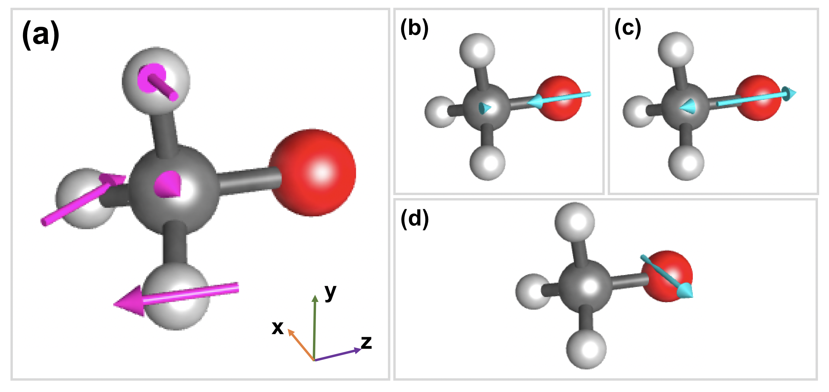
Figure 1: (a) [Magenta] The displacements of the first vibrational mode along which we propagate dynamics. In (b), we plot [cyan] the atom-based spin magnetic moments for a single GHF+SOC solution, and in (c) we plot the corresponding moments for its degenerate time-reversed solution. (d) The weighted spin magnetic moments on each atom using the initial amplitude $\bm{c}=(\frac{1}{\sqrt{2}},\frac{i}{\sqrt{2}})$.

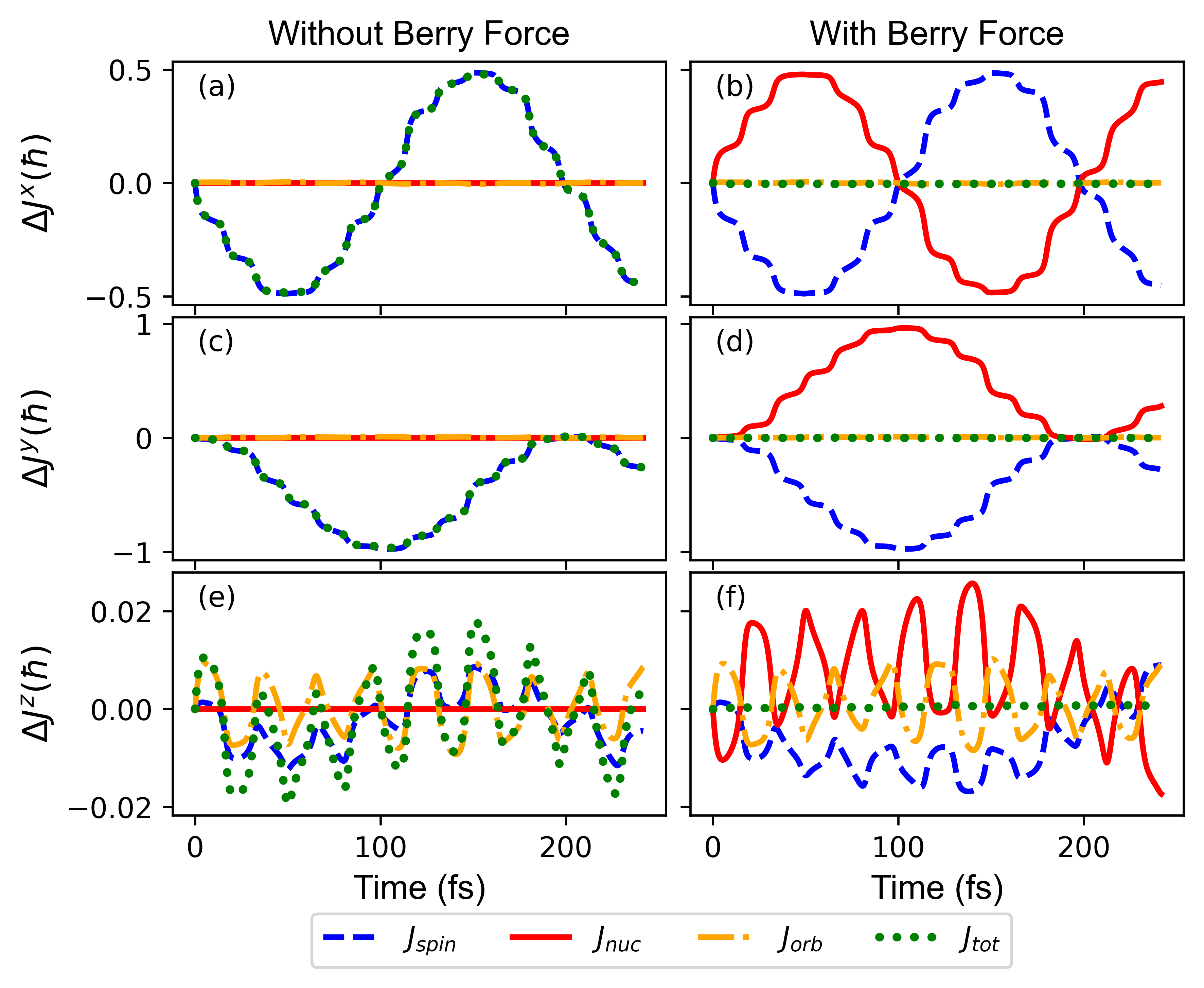
Figure 2: The change in the real-time angular momentum $\Delta J^{\alpha}(t)=J^{\alpha}(t)-J^{\alpha}(0)$ (relative to time zero) according to an Ehrenfest trajectory simulating methoxy radical moving along its lowest normal mode vibration. The nonzero initial values of components of the angular momentum are listed: $J^{y}_{\rm spin}=0.4811\hbar$, $J^{y}_{\rm orb}=-0.0054\hbar$, $J^{\rm x}_{\rm nuc}=0.0075\hbar$, and $J^{\rm z}_{\rm nuc}=-0.0048\hbar$. The three panels (a),(c),(e) on the left exclude the non-Abelian Berry force and correspond to the Cartesian coordinates $x$, $y$ and $z$ shown in Fig. 1 (and the same for Figs.(b),(d) and (f) but now including the Berry force). Without a Berry force, the total angular momentum is not conserved; with a Berry force, the total angular momentum is conserved. In Figs.(b) and (d), when we correctly include the Berry force, we find that the nuclear and spin degrees of freedom transfer angular momentum between each other. In Figs (f), the nuclear, spin, and electronic orbital degrees of freedom all exchange angular momentum. Comparing (e) and (f), we observe that the electronic spin changes differently with or without a Berry force; this change arises because adding the Berry force can changes the nuclear motion and yields a reasonably different trajectory.

In Fig.2, we plot the change in the angular momentum and linear momentum during the trajectory. To begin our discussion, consider first the case where Berry force is not included (Fig.2(a)(c)(e))). When the Berry force is not included, the nuclear angular momentum is calculated from the canonical momentum $\bm{P}_{\rm n}$, which is conserved for a translationally invariant surface, and hence there is no change in the nuclear momentum (red solid line). Note that the canonical momentum is conserved in this example because the two basis states are degenerate. In the more general case, with multiple non-degenerate states, the canonical momentum would not be conserved, as shown previously in Ref.Shu et al. (2020). In blue, we pot the electronic spin angular momentum; in orange, we plot the electronic orbital angular momentum. In Fig.2(a) and (c), the electronic spin angular momentum changes tracks exactly with the total angular momentum (i.e. the electronic orbital angular momentum is effectively constant). In Fig.2(e), both the electronic orbital and spin angular momentum fluctuate, and the total angular momentum appears more chaotic.

Next, consider Fig.2(b)(d)(f)) where the Berry force is included. Here, we see the nuclear angular momentum (as calculated from the kinetic momentum $\bm{\pi}_{\rm n}$ in Eq. 71) changes with time, and the Berry force captures the angular momentum transfer from the electronic spin/orbital angular momentum to the nuclear angular momentum. As must be true, the total angular momentum is constant and conserved. (In Fig.S2, we also show numerically that the total linear momentum is conserved when a Berry force is included.) Of most importance, when comparing Figs. 2(e) and (f), we observe that the electronic spin changes noticeably depending on whether or not a Berry force is included, clearly emphasizing the importance of going beyond standard BO dynamics (and including Berry forces) in the presence of non-trivial spin degrees of freedom.

VII Discussion

VII.1 Choice of Phase/Gauge $\xi$

At this point, it is essential for us to discuss our choice of phase. For the case of a real Hamiltonian, one can choose the Hamiltonian eigenfunctions to be real as well (in a smooth fashion), and thus one can ignore the gauge choice $\xi$ in Eqs. 25-26. However, in the case of a complex-valued Hamiltonian, the choice of phase is far more complicated. Obviously, Berry phases can appear (which should not be ignored) if one moves around in a closed loopBerry (1984). Even more importantly for our semiclassical purposes, the choice of phase will always be somewhat uncontrollable for ab initio on-the-fly dynamics because one must pick the phase of the resulting wavefunction at each step with very limited information: one does not have the capacity to make sure that the phases of wavefunctions are matched for similar nuclear configurations and one cannot easily attach different phase factors for translational, rotational, and internal motion. Thus, at the end of the day, for the most part, the usual approach is simply to align the phases of nuclear wavefunctions at two slightly different geometries (separated by one time step) using parallel transport. Parallel transport does not satisfy $\xi=0$ in Eqs. 25-26. Therefore, when running semiclassical dynamics, one seeks equations of motion that are insensitive to the gauge and to that end, as a practical matter, the Ehrenfest equations in Eqs. 68-71 have a huge advantage over those in Eqs. 84-85.

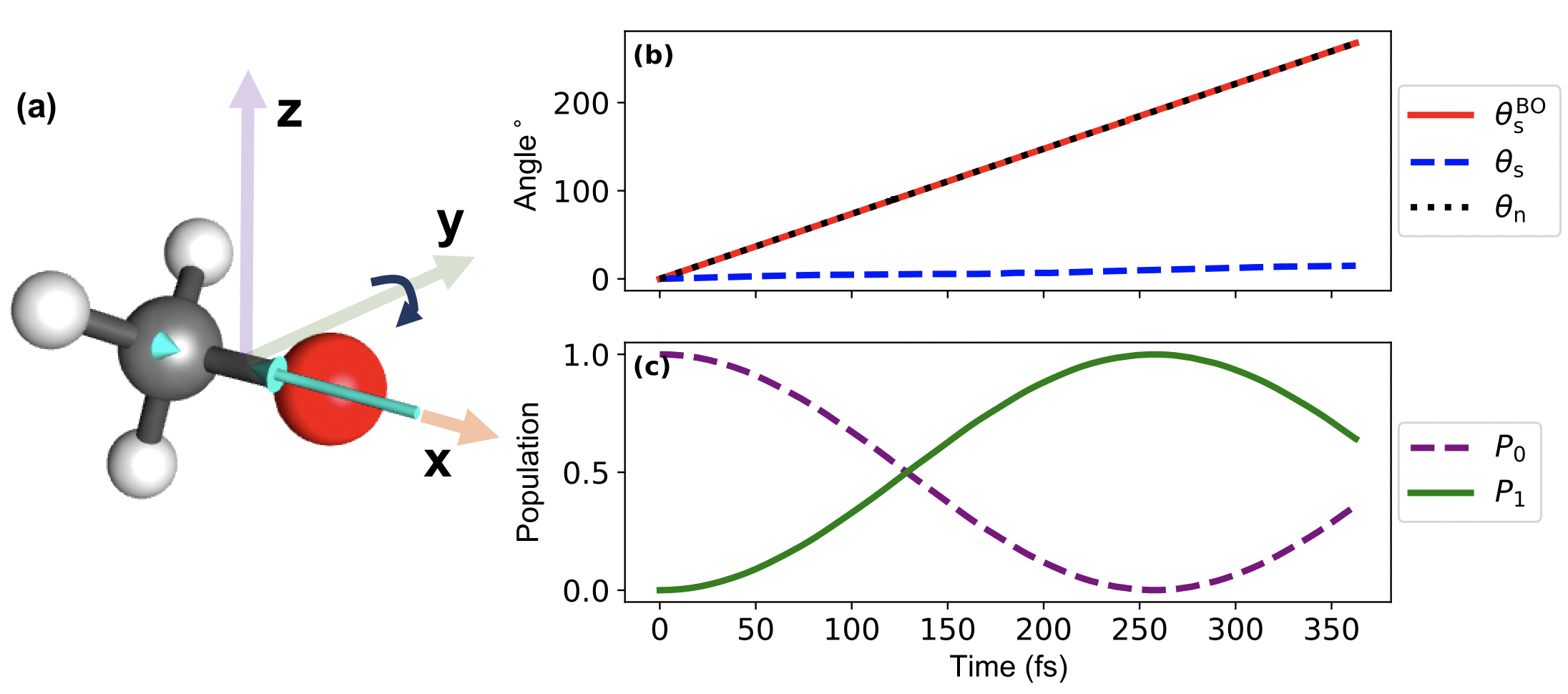
Figure 3: (a) The orientation of the methoxy radical molecule, the rotation direction, and atom-based spin magnetic moments (cyan arrows) at the initial step. (b) The rotation angles of the molecule (black dotted line), the total spin vector from the BO dynamics (red solid line), and from the Ehrenfest dynamics (blue dashed lines). (c) The populations for the Kramers doublet states ($P_{0}$ and $P_{1}$) with time from the Ehrenfest dynamics.

VII.2 Ehrenfest vs BO Dyanmics

Lastly, before concluding, in order to numerically emphasize the need to go beyond the BO approximation when treating spin spin degrees of freedom, we will report one more simulation. Let us orient the methoxy radical molecule with the CO bond aligned along the x axis; within such a frame, a GHF calculation with SOC reveals that all spin magnetic moments point along the x-axis (Fig. 3(a)). Let us now apply a rotational force around the y axis, with the initial nuclear angular momentum $J_{\rm nuc}=(0.0,39.28\hbar,0.0)$, and propagate the resulting dynamics with both BO and Ehrenfest. For both sets of dynamics, we include the corresponding Berry force (the on-diagonal Berry force for BO dynamicsTao, Qiu, and Subotnik (2023); Bian et al. (2023) and the non-Abelian Berry force Amano and Takatsuka (2005); Krishna (2007) for Ehrenfest dynamics), so that both trajectories conserve the total angular momentum. For additional trajectory data, and in particular for the time-dependent state populations and an analysis of the spin angular momentum in terms of the relevant $\ket{GHF}$ and $\ket{TGHF}$ wavefunctions, see the SI. In Fig. 3(b), as a function of time, we plot the rotation angle for the molecule as well as the total expectation values for the spin vectors according to both BO and Ehrenfest dynamics. As one might expect, within the BO approximation (as calculated along a continuous GHF+SOC state), the total spin vector $\textbf{S}_{\rm BO}$ rotates with the molecule (red line).This prediction is of course unphysical, however; the spin direction does not change instantaneously with molecular frame but rather changes depending on the spin-orbit coupling. This slow change of direction is correctly captured by Ehrenfest dynamics (blue dashed lines). Lastly, this BO failure can be verified in 3(c), where we plot population as a function of time and show, the time the molecule has rotated 180 degrees (244 fs), the populated Kramers doublet has effectively switched, which represents a complete breakdown of the BO approximation.

VIII Conclusions

In this paper, we have demonstrated that, in order for Ehrenfest dynamics to conserve the linear or angular momentum in a truncated basis, the nuclei must experience a force arising from the non-Abelian curvature $\bm{\Omega}$ (as present in Eqs. 68-71). This result is independent of the choice of gauge for the electronic states in Eqs. 25-26. As examples, we have studied both the traveling hydrogen atom (analytically) as well as the methoxy radical (numerically). Both examples make clear that the non-Abelian curvature term is needed and, in the case of the methoxy radical, our data also highlights that the evolution of the spin degrees of freedom can be different as a result. Looking forward, the present results should have immediate impact in a variety of fields where nuclear, electronic and spin motion are all entangled perhaps especially for systems displaying chiral-induced spin selectivityDas et al. (2022); Evers et al. (2022).

IX Supplementary Material

In the supplementary material, we include a proof of Eqs.40 and LABEL:eq:Jvanish, a proof of the gauge covariance of the non-Abelian berry curvature (Eq.83), a detailed discussion of the alternative Ehrenfest scheme in Eqs.84-85 vis-a-vis momentum conservation, and more details of the methoxy radical dynamics.

X Acknowledgment

We would like to thank Tanner Culpitt for a careful reading. This work is supported by the National Science Foundation under Grant No. CHE-2102402.

References

• Amano and Takatsuka (2005) M. Amano and K. Takatsuka, “Quantum fluctuation of electronic wave-packet dynamics coupled with classical nuclear motions,” The Journal of Chemical Physics 122 (2005), 10.1063/1.1854115.
• Krishna (2007) V. Krishna, “Path integral formulation for quantum nonadiabatic dynamics and the mixed quantum classical limit,” The Journal of Chemical Physics 126 (2007), 10.1063/1.2716387.
• Nelson et al. (2014) T. Nelson, S. Fernandez-Alberti, A. E. Roitberg,  and S. Tretiak, “Nonadiabatic excited-state molecular dynamics: Modeling photophysics in organic conjugated materials,” Accounts of Chemical Research 47, 1155–1164 (2014).
• Tully (1998) J. C. Tully, “Mixed quantum–classical dynamics,” Faraday Discussions 110, 407–419 (1998).
• Egorov, Rabani, and Berne (1999) S. A. Egorov, E. Rabani,  and B. J. Berne, “On the adequacy of mixed quantum-classical dynamics in condensed phase systems,” The Journal of Physical Chemistry B 103, 10978–10991 (1999).
• Kapral and Ciccotti (1999) R. Kapral and G. Ciccotti, “Mixed quantum-classical dynamics,” The Journal of Chemical Physics 110, 8919–8929 (1999).
• Curchod, Rothlisberger, and Tavernelli (2013) B. F. E. Curchod, U. Rothlisberger,  and I. Tavernelli, “Trajectory-based nonadiabatic dynamics with time-dependent density functional theory,” ChemPhysChem 14, 1314–1340 (2013).
• Römer and Burghardt (2013a) S. Römer and I. Burghardt, “Towards a variational formulation of mixed quantum-classical molecular dynamics,” Molecular Physics 111, 3618–3624 (2013a).
• Crespo-Otero and Barbatti (2018) R. Crespo-Otero and M. Barbatti, “Recent advances and perspectives on nonadiabatic mixed quantum–classical dynamics,” Chemical Reviews 118, 7026–7068 (2018).
• Tully (1990) J. C. Tully, “Molecular dynamics with electronic transitions,” The Journal of Chemical Physics 93, 1061–1071 (1990).
• Barbatti (2011) M. Barbatti, “Nonadiabatic dynamics with trajectory surface hopping method,” WIREs Computational Molecular Science 1, 620–633 (2011).
• Wang, Akimov, and Prezhdo (2016) L. Wang, A. Akimov,  and O. V. Prezhdo, “Recent progress in surface hopping: 2011–2015,” The Journal of Physical Chemistry Letters 7, 2100–2112 (2016).
• Subotnik et al. (2016) J. E. Subotnik, A. Jain, B. Landry, A. Petit, W. Ouyang,  and N. Bellonzi, “Understanding the surface hopping view of electronic transitions and decoherence,” Annual Review of Physical Chemistry 67, 387–417 (2016).
• Wu et al. (2022) Y. Wu, X. Bian, J. I. Rawlinson, R. G. Littlejohn,  and J. E. Subotnik, “A phase-space semiclassical approach for modeling nonadiabatic nuclear dynamics with electronic spin,” The Journal of Chemical Physics 157, 011101 (2022).
• Micha (1983) D. A. Micha, “A self-consistent eikonal treatment of electronic transitions in molecular collisions,” The Journal of Chemical Physics 78, 7138–7145 (1983).
• Billing (1983) G. D. Billing, “On the use of ehrenfest’s theorem in molecular scattering,” Chemical Physics Letters 100, 535–539 (1983).
• Sawada, Nitzan, and Metiu (1985) S.-I. Sawada, A. Nitzan,  and H. Metiu, “Mean-trajectory approximation for charge- and energy-transfer processes at surfaces,” Physical Review B 32, 851–867 (1985).
• Li et al. (2005) X. Li, J. C. Tully, H. B. Schlegel,  and M. J. Frisch, “Ab initio ehrenfest dynamics,” The Journal of Chemical Physics 123, 084106 (2005).
• Meyer and Miller (1979) H. Meyer and W. H. Miller, “A classical analog for electronic degrees of freedom in nonadiabatic collision processes,” The Journal of Chemical Physics 70, 3214–3223 (1979).
• Andrew et al. (2004) P. H. Andrew, D. R. Bowler, A. J. Fisher, N. T. Tchavdar,  and G. S. Cristián, “Beyond ehrenfest: correlated non-adiabatic molecular dynamics,” Journal of Physics: Condensed Matter 16, 8251 (2004).
• Parandekar and Tully (2005) P. V. Parandekar and J. C. Tully, “Mixed quantum-classical equilibrium,” The Journal of Chemical Physics 122 (2005), 10.1063/1.1856460.
• Parandekar and Tully (2006) P. V. Parandekar and J. C. Tully, “Detailed balance in ehrenfest mixed quantum-classical dynamics,” Journal of Chemical Theory and Computation 2, 229–235 (2006).
• Curchod and Martínez (2018) B. F. E. Curchod and T. J. Martínez, “Ab initio nonadiabatic quantum molecular dynamics,” Chemical Reviews 118, 3305–3336 (2018).
• Esch and Levine (2020) M. P. Esch and B. G. Levine, “Decoherence-corrected ehrenfest molecular dynamics on many electronic states,” The Journal of Chemical Physics 153 (2020), 10.1063/5.0022529.
• Esch and Levine (2021) M. P. Esch and B. Levine, “An accurate, non-empirical method for incorporating decoherence into ehrenfest dynamics,” The Journal of Chemical Physics 155 (2021), 10.1063/5.0070686.
• Shu and Truhlar (2023) Y. Shu and D. G. Truhlar, “Decoherence and its role in electronically nonadiabatic dynamics,” Journal of Chemical Theory and Computation 19, 380–395 (2023).
• Fedorov and Levine (2019) D. A. Fedorov and B. G. Levine, “Nonadiabatic quantum molecular dynamics in dense manifolds of electronic states,” The Journal of Physical Chemistry Letters 10, 4542–4548 (2019).
• Shalashilin (2009) D. V. Shalashilin, “Quantum mechanics with the basis set guided by ehrenfest trajectories: Theory and application to spin-boson model,” The Journal of Chemical Physics 130 (2009), 10.1063/1.3153302.
• Römer and Burghardt (2013b) S. Römer and I. Burghardt, “Towards a variational formulation of mixed quantum-classical molecular dynamics,” Molecular Physics 111, 3618–3624 (2013b).
• Zhu et al. (2004) C. Zhu, S. Nangia, A. W. Jasper,  and D. G. Truhlar, “Coherent switching with decay of mixing: An improved treatment of electronic coherence for non-born–oppenheimer trajectories,” The Journal of Chemical Physics 121, 7658–7670 (2004).
• Zhu, Jasper, and Truhlar (2004) C. Zhu, A. W. Jasper,  and D. G. Truhlar, “Non-born–oppenheimer trajectories with self-consistent decay of mixing,” The Journal of Chemical Physics 120, 5543–5557 (2004).
• Akimov, Long, and Prezhdo (2014) A. V. Akimov, R. Long,  and O. V. Prezhdo, “Coherence penalty functional: A simple method for adding decoherence in ehrenfest dynamics,” The Journal of chemical physics 140 (2014).
• Isborn, Li, and Tully (2007) C. M. Isborn, X. Li,  and J. C. Tully, “Time-dependent density functional theory ehrenfest dynamics: Collisions between atomic oxygen and graphite clusters,” The Journal of Chemical Physics 126 (2007), 10.1063/1.2713391.
• Note (1) Energy conservation and frustrated hops are of course the reasons that Tully’s algorithm approximately obeys detailed balance.
• Littlejohn, Rawlinson, and Subotnik (2023) R. Littlejohn, J. Rawlinson,  and J. Subotnik, “Representation and conservation of angular momentum in the born–oppenheimer theory of polyatomic molecules,” The Journal of Chemical Physics 158, 104302 (2023).
• Bian et al. (2023) X. Bian, Z. Tao, Y. Wu, J. Rawlinson,  and J. E. S. Robert G Littlejohn, “Total angular momentum conservation in ab initio born-oppenheimer molecular dynamics,” arXiv preprint arXiv:2303.13787  (2023).
• Abedi, Maitra, and Gross (2010) A. Abedi, N. T. Maitra,  and E. K. U. Gross, “Exact factorization of the time-dependent electron-nuclear wave function,” Physical Review Letters 105, 123002 (2010).
• Abedi, Maitra, and Gross (2012) A. Abedi, N. T. Maitra,  and E. K. U. Gross, “Correlated electron-nuclear dynamics: Exact factorization of the molecular wavefunction,” The Journal of Chemical Physics 137, 22A530 (2012).
• Vindel-Zandbergen, Matsika, and Maitra (2022) P. Vindel-Zandbergen, S. Matsika,  and N. T. Maitra, “Exact-factorization-based surface hopping for multistate dynamics,” The Journal of Physical Chemistry Letters 13, 1785–1790 (2022).
• Li, Requist, and Gross (2022) C. Li, R. Requist,  and E. K. U. Gross, “Energy, momentum, and angular momentum transfer between electrons and nuclei,” Physical Review Letters 128, 113001 (2022).
• Shu et al. (2020) Y. Shu, L. Zhang, Z. Varga, K. A. Parker, S. Kanchanakungwankul, S. Sun,  and D. G. Truhlar, “Conservation of angular momentum in direct nonadiabatic dynamics,” The Journal of Physical Chemistry Letters 11, 1135–1140 (2020).
• Mead (1992) C. A. Mead, “The geometric phase in molecular systems,” Reviews of Modern Physics 64, 51–85 (1992).
• Doltsinis (2002) N. Doltsinis, “Nonadiabatic dynamics: Mean-field and surface hopping,” in Quantum Simulations of Complex Many-Body Systems: From Theory to Algorithms, edited by J. Grotendorst, D. Marx,  and A. Muramatsu (John von Neumann Inst. Comput., 2002) pp. 377–397.
• Wilczek and Zee (1984) F. Wilczek and A. Zee, “Appearance of gauge structure in simple dynamical systems,” Physical Review Letters 52, 2111 (1984).
• Miller (2009) W. H. Miller, “Electronically nonadiabatic dynamics via semiclassical initial value methods,” Journal of Physical Chemistry A 113, 1405 (2009).
• McLachlan (1961) A. D. McLachlan, “The wave functions of electronically degenerate states,” Molecular Physics 4, 417–423 (1961).
• Mead and Truhlar (1982) C. A. Mead and D. G. Truhlar, “Conditions for the definition of a strictly diabatic electronic basis for molecular systems,” The Journal of Chemical Physics 77, 6090–6098 (1982).
• Jasper et al. (2004) A. W. Jasper, B. K. Kendrick, C. A. Mead,  and D. G. Truhlar, “Non-born-oppenheimer chemistry: Potential surfaces, couplings, and dynamics,” in Modern Trends in Chemical Reaction Dynamics (2004) pp. 329–391.
• Cotton, Liang, and Miller (2017) S. J. Cotton, R. Liang,  and W. H. Miller, “On the adiabatic representation of meyer-miller electronic-nuclear dynamics,” The Journal of Chemical Physics 147 (2017), 10.1063/1.4995301.
• Takatsuka (2007) K. Takatsuka, “Generalization of classical mechanics for nuclear motions on nonadiabatically coupled potential energy surfaces in chemical reactions,” The Journal of Physical Chemistry A 111, 10196–10204 (2007).
• Yonehara and Takatsuka (2008) T. Yonehara and K. Takatsuka, “Nonadiabatic electron wavepacket dynamics of molecules in an intense optical field: An ab initio electronic state study,” The Journal of Chemical Physics 128 (2008), 10.1063/1.2904867.
• Takatsuka (2017) K. Takatsuka, “Lorentz-like force emerging from kinematic interactions between electrons and nuclei in molecules: A quantum mechanical origin of symmetry breaking that can trigger molecular chirality,” The Journal of Chemical Physics 146 (2017), 10.1063/1.4976976.
• Fatehi et al. (2011) S. Fatehi, E. Alguire, Y. Shao,  and J. E. Subotnik, “Analytic derivative couplings between configuration-interaction-singles states with built-in electron-translation factors for translational invariance,” The Journal of Chemical Physics 135, 234105 (2011).
• Athavale et al. (2023) V. Athavale, X. Bian, Z. Tao, Y. Wu, T. Qiu, J. Rawlinson, R. G. Littlejohn,  and J. E. Subotnik, “Surface hopping, electron translation factors, electron rotation factors, momentum conservation, and size consistency,” The Journal of Chemical Physics 159 (2023), 10.1063/5.0160965.
• Nafie (1983) L. A. Nafie, “Adiabatic molecular properties beyond the born–oppenheimer approximation. complete adiabatic wave functions and vibrationally induced electronic current density,” The Journal of Chemical Physics 79, 4950–4957 (1983).
• Patchkovskii (2012) S. Patchkovskii, “Electronic currents and born-oppenheimer molecular dynamics,” The Journal of Chemical Physics 137 (2012), 10.1063/1.4747540.
• Abegg (1975) P. W. Abegg, “Ab initio calculation of spin-orbit coupling constants for gaussian lobe and gaussian-type wave functions,” Mol. Phys. 30, 579–596 (1975).
• Tao, Qiu, and Subotnik (2023) Z. Tao, T. Qiu,  and J. E. Subotnik, “Symmetric post-transition state bifurcation reactions with berry pseudomagnetic fields,” The Journal of Physical Chemistry Letters 14, 770–778 (2023).
• Kubler et al. (1988) J. Kubler, K. H. Hock, J. Sticht,  and A. R. Williams, “Density functional theory of non-collinear magnetism,” Journal of Physics F: Metal Physics 18, 469 (1988).
• Epifanovsky et al. (2021) E. Epifanovsky, A. T. B. Gilbert, X. Feng, J. Lee, Y. Mao, N. Mardirossian, P. Pokhilko, A. F. White, M. P. Coons, A. L. Dempwolff, Z. Gan, D. Hait, P. R. Horn, L. D. Jacobson, I. Kaliman, J. Kussmann, A. W. Lange, K. U. Lao, D. S. Levine, J. Liu, S. C. McKenzie, A. F. Morrison, K. D. Nanda, F. Plasser, D. R. Rehn, M. L. Vidal, Z.-Q. You, Y. Zhu, B. Alam, B. J. Albrecht, A. Aldossary, E. Alguire, J. H. Andersen, V. Athavale, D. Barton, K. Begam, A. Behn, N. Bellonzi, Y. A. Bernard, E. J. Berquist, H. G. A. Burton, A. Carreras, K. Carter-Fenk, R. Chakraborty, A. D. Chien, K. D. Closser, V. Cofer-Shabica, S. Dasgupta, M. de Wergifosse, J. Deng, M. Diedenhofen, H. Do, S. Ehlert, P.-T. Fang, S. Fatehi, Q. Feng, T. Friedhoff, J. Gayvert, Q. Ge, G. Gidofalvi, M. Goldey, J. Gomes, C. E. González-Espinoza, S. Gulania, A. O. Gunina, M. W. D. Hanson-Heine, P. H. P. Harbach, A. Hauser, M. F. Herbst, M. H. Vera, M. Hodecker, Z. C. Holden, S. Houck, X. Huang, K. Hui, B. C. Huynh, M. Ivanov, Ádám Jász, H. Ji, H. Jiang, B. Kaduk, S. Kähler, K. Khistyaev, J. Kim, G. Kis, P. Klunzinger, Z. Koczor-Benda, J. H. Koh, D. Kosenkov, L. Koulias, T. Kowalczyk, C. M. Krauter, K. Kue, A. Kunitsa, T. Kus, I. Ladjánszki, A. Landau, K. V. Lawler, D. Lefrancois, S. Lehtola, et al., “Software for the frontiers of quantum chemistry: An overview of developments in the q-chem 5 package,” The Journal of Chemical Physics 155, 084801 (2021).
• Jiménez-Hoyos, Rodríguez-Guzmán, and Scuseria (2014) C. A. Jiménez-Hoyos, R. Rodríguez-Guzmán,  and G. E. Scuseria, “Polyradical character and spin frustration in fullerene molecules: An ab initio non-collinear hartree–fock study,” The Journal of Physical Chemistry A 118, 9925–9940 (2014).
• Berry (1984) M. V. Berry, “Quantal phase factors accompanying adiabatic changes,” Proceedings of the Royal Society of London. A. Mathematical and Physical Sciences 392, 45–57 (1984).
• Das et al. (2022) T. K. Das, F. Tassinari, R. Naaman,  and J. Fransson, “Temperature-dependent chiral-induced spin selectivity effect: Experiments and theory,” The Journal of Physical Chemistry C 126, 3257–3264 (2022).
• Evers et al. (2022) F. Evers, A. Aharony, N. Bar-Gill, O. Entin-Wohlman, P. Hedegård, O. Hod, P. Jelinek, G. Kamieniarz, M. Lemeshko, K. Michaeli, V. Mujica, R. Naaman, Y. Paltiel, S. Refaely-Abramson, O. Tal, J. Thijssen, M. Thoss, J. M. van Ruitenbeek, L. Venkataraman, D. H. Waldeck, B. Yan,  and L. Kronik, “Theory of chirality induced spin selectivity: Progress and challenges,” Advanced Materials 34, 2106629 (2022).