Asteroseismology of the young open cluster NGC 2516 I: Photometric and spectroscopic observations

Abstract

Context. Asteroseismic modelling of isolated stars presents significant challenges due to the difficulty in accurately determining stellar parameters, particularly the stellar age. These challenges can be overcome by observing stars in open clusters, whose coeval members share an initial chemical composition. The light curves from the all-sky survey by the Transiting Exoplanet Survey Satellite (TESS) allow us to investigate and analyse stellar variations in clusters with an unprecedented level of detail for the first time.

Aims. We aim to detect gravity-mode oscillations in the early-type main-sequence members of the young open cluster NGC 2516 to deduce their internal rotation rates.

Methods. We selected the 301 of member stars with no more than mild contamination as our sample. We analysed the full-frame image (FFI) light curves, which provide nearly continuous observations in the first and third years of TESS monitoring. We also collected high-resolution spectra using the Fiber-fed Extended Range Optical Spectrograph (FEROS) for the g-mode pulsators, with the aim to assess the Gaia effective temperatures and gravities, and to prepare for future seismic modelling.

Results. By fitting the theoretical isochrones to the colour-magnitude diagram (CMD) of a cluster, we determined an age of $102\pm 15$ Myr and inferred the extinction at 550 nm ($A_{0}$) is $0.53\pm 0.04$ mag. We identified 147 stars with surface brightness modulations, 24 with gravity (g-)mode pulsations ($\gamma$ Doradus or Slowly Pulsating B stars), and 35 with pressure (p-)mode pulsations ($\delta$ Sct stars). When sorted by colour index, the amplitude spectra of the $\delta$ Sct stars show a distinct ordering and reveal a discernible frequency-temperature relationship. The near-core rotation rates, measured from period spacing patterns in two SPB and nine $\gamma$ Dor stars, reach up to $3\,\mathrm{d^{-1}}$. This is at the high end of the values found from Kepler data of field stars of similar variability type. The $\gamma$ Dor stars of NGC 2516 have internal rotation rates as high as 50% of their critical value, whereas the SPB stars exhibit rotation rates close to their critical rate. Although the B-type stars are rotating rapidly, we did not find long-term brightness and colour variations in the mid-infrared, which suggests that there are no disk or shell formation events in our sample. We also discussed the results of our spectroscopic observations for the g-mode pulsators.

1 Introduction

Clusters serve as excellent laboratories for stellar astrophysics due to the advantage that member stars within the same cluster typically share similar distance, age, and initial metallicity. Nevertheless, recent studies have complicated these notions: some works reveal extended coronae in nearby star clusters, where their sizes greatly exceed those of their cluster cores (Meingast & Alves, 2019; Meingast et al., 2021; Bouma et al., 2021). Furthermore, both globular and open clusters have shown evidence of multiple populations, indicating complex star formation histories (Gratton et al., 2012; Li et al., 2016; Wang et al., 2022). Additionally, uncertainties arise in stellar evolutionary tracks and isochrones due to the complex input physics and poor calibration of stellar models (e.g. Martins & Palacios, 2013).

Rotation, a process of stellar physics that remains poorly calibrated, plays a crucial role in stellar evolution, as recognised for many decades (e.g. Shajn & Struve, 1929; Maeder, 2009). For instance, rotation enhances element mixing and transports more fuel to the core, resulting in increased luminosity and extended lifetimes. Rapid rotation also causes a star to become oblate and generates a surface temperature gradient, affecting the observed colour and brightness (e.g. von Zeipel, 1924; Zahn et al., 2010; Espinosa Lara & Rieutord, 2011; Bouchaud et al., 2020, known as the gravity darkening effect). Consequently, the rotational effects strongly influence the locations of stars on the colour-magnitude diagram (CMD), leading to scatter in the observed CMD. Therefore, rotation is considered the most plausible mechanism for the extended main-sequence turn-off (eMSTO) phenomenon (e.g. Bertelli et al., 2003; Glatt et al., 2009; Bastian & de Mink, 2009; Girardi et al., 2013; Correnti et al., 2015; D’Antona et al., 2015; Brandt & Huang, 2015; Bastian et al., 2016, 2018; Li et al., 2019a; Gossage et al., 2019; Lim et al., 2019, among many other studies).

There is a limited availability of observed rotation rates for hot eMSTO stars, but numerous surface rotation measurements are available for cool main-sequence stars (spectral class F8V or later, Kraft, 1967). The rotation rates of these cool stars can be easily and accurately measured through their surface modulations (e.g. McQuillan et al., 2014). These observations have paved the way for gyrochronology, a method that determines the ages of cool main-sequence stars based on their masses and rotation rates, while other physical properties remain relatively unchanged during their long main-sequence stage (Skumanich, 1972; Barnes, 2003, 2007). However, gyrochronology is not applicable to hot main-sequence stars since they lack thick convective envelopes, resulting in no or weak magnetic braking. Consequently, hot main-sequence stars tend to rotate rapidly, with surface rotation frequencies of the order of $1\,\mathrm{d^{-1}}$ or $v\sin i\sim 100\,\mathrm{km/s}$ (Royer et al., 2007; Li et al., 2020b). For these stars, surface modulation is often absent or weak, but their internal rotation rates can be obtained through asteroseismology.

Asteroseismology, the field dedicated to the interpretation of stellar oscillations, has proven to be a potent tool for peering into the interior physics of stars (e.g., Aerts, 2021). The fundamental concept revolves around standing waves that penetrate different layers of stars. These waves undergo modifications due to the local environment such as sound speed and density. Consequently, the eigenfrequencies carry information about the internal structure of stars (for more detailed information, we refer to textbooks such as Unno et al., 1989; Aerts et al., 2010; Basu & Chaplin, 2017). Notably, the temperature range at which gyrochronology loses its effectiveness aligns with the cool boundary of the classical instability strip (IS) for pulsating stars (roughly from 7000 to 10000 K, where $\delta$ Scuti ($\delta$ Sct) stars and $\gamma$ Doradus ($\gamma$ Dor) stars reside Dupret et al., 2005; Bouabid et al., 2013; Xiong et al., 2016; Murphy et al., 2019). Slowly Pulsating B-type (SPB) stars and $\beta$ Cephei ($\beta$ Cep) stars appear at higher temperature ranges (hotter than $\sim$10000 K). As a result, various types of pulsating stars are being studied asteroseismically, which are hotter than Sun-like stars with solar-like oscillations.

At the temperature range of eMSTO in young open clusters, stars more massive than the Sun are the main objects for asteroseismology. Some of these stars pulsate in pressure (p) modes, including $\beta$ Cep stars (Sterken & Jerzykiewicz, 1993; Aerts & De Cat, 2003) and $\delta$ Sct stars (Goupil et al., 2005; Handler, 2009; Bedding et al., 2020). These modes are particularly sensitive to the outer envelopes of stars. Conversely, some stars pulsate in gravity (g) modes, like $\gamma$ Dor stars (Balona et al., 1994; Kaye et al., 1999; Van Reeth et al., 2015c) and SPB stars (Waelkens, 1991; De Cat & Aerts, 2002; Pedersen et al., 2021), allowing us to probe deeper into the stellar structure, reaching down to the boundary of the convective core. The Gaia space mission confirmed that many pulsating stars exist between the SPB and $\delta$ Sct instability strips (Gaia Collaboration et al., 2023a).

The excitation mechanisms behind the pulsations in this part of the Hertzsprung-Russell diagram (HRD) are primarily the $\kappa$ mechanism (Pamyatnykh, 1999) with contributions from turbulent pressure (Houdek, 2000; Antoci et al., 2014) and the so-called edge-bump mechanism (Stellingwerf, 1979; Murphy et al., 2020). Less understood is the interplay with damping mechanisms as a function of the various input physics, such as transport processes induced by rotation and magnetism (e.g., Mathis, 2013; Aerts et al., 2019). A main goal of asteroseismology is to better understand this, starting with a well-characterised sample that can be accurately modelled. From an observational perspective, the ability to detect non-radial pulsators all along the main sequence significantly broadens the temperature coverage for such asteroseismic investigations (Kurtz et al., 2023).

Research on internal stellar rotation is the most attractive topic among many of those driven by asteroseismology, with large progress in stellar physics based on rotationally induced processes (Aerts et al., 2019). Rotation lifts the degeneracy among mode frequencies, splitting modes into multiplets (Ledoux, 1951). Rotational splittings have been observed in many kinds of variable stars, such as the Sun (Deubner et al., 1979), white dwarfs (Winget et al., 1991), subdwarfs (Reed et al., 2000), $\beta\,$Cep stars (Aerts et al., 2003), slowly-rotating $\gamma$ Dor and SPB stars (Pápics et al., 2014; Kurtz et al., 2014; Saio et al., 2015; Murphy et al., 2016; Li et al., 2019b), and red giant stars (e.g. Mosser et al., 2012; Deheuvels et al., 2014; Gehan et al., 2018). The splittings observed from different p or g modes carry information on rotation rates in different stellar layers, providing the possibility to re-construct core-to-surface differential rotation profiles (Corbard et al., 1999; Deheuvels et al., 2014, 2015; Triana et al., 2015; Di Mauro et al., 2016; Triana et al., 2017; Deheuvels et al., 2020).

Many of the variable stars situated in hot eMSTOs rotate rapidly, notably with a rotation frequency close to the frequencies of g modes. Such modes are often in the sub-inertial regime of the frequency range (Aerts et al., 2019) and are gravito-inertial modes. The traditional approximation of rotation (TAR) offers an appropriate formalism to treat the rotational effects properly when computing such mode frequencies (Lee & Saio, 1987, 1997; Townsend, 2003; Mathis, 2009; Van Reeth et al., 2016; Saio et al., 2018). Under the approximation of the TAR, the mode period spacing $\Delta P\equiv P_{n+1,l,m}-P_{n,l,m}$, defined as the period difference of two modes with consecutive radial order $n$ but the same angular degree $l$ and azimuthal order $m$, is no longer constant as predicted by asymptotic theory (Shibahashi, 1979). Instead, the period spacings exhibit decreasing or increasing trends as a function of period, depending on the mode identification (Bouabid et al., 2013; Van Reeth et al., 2015a; Ouazzani et al., 2017). Prograde ($m=1$) dipole ($l=1$) modes are the most common in real observations and have been observed in hundreds of $\gamma$ Dor or tens of SPB stars (Li et al., 2020b; Pedersen et al., 2021). They show decreasing period spacings with increasing period and allow us to measure the stars’ near-core rotation rates and calibrate internal mixing processes (Van Reeth et al., 2016; Li et al., 2020b; Szewczuk & Daszyńska-Daszkiewicz, 2018; Pedersen et al., 2021; Mombarg et al., 2021). Recently discovered coupling between an inertial mode in the convective core and a gravito-inertial mode in the envelope has opened a new window for exploring the rotation and internal physics of convective cores, where g modes do not propagate (Ouazzani et al., 2020; Saio et al., 2021; Tokuno & Takata, 2022; Aerts & Mathis, 2023).

Our primary aim is to compile a comprehensive list of various types of pulsating stars within NGC 2516, which is a bright, young, and solar-metallicity open cluster. In this study, we analysed space photometry of the members of NGC 2516 from the Transiting Exoplanet Survey Satellite (TESS) mission (Ricker et al., 2015) and conducted high-resolution spectroscopic follow-up observations of the g-mode pulsators in the open cluster NGC 2516. The paper is organized as follows: Section 2 introduces the basic information of NGC 2516 and the sample selection criteria. Section 3 discusses the fitting of theoretical isochrones to the observed CMD. The TESS photometry and the research on variable stars are presented in Sect. 4. Spectroscopic observations and results are described in Sect. 5. Finally, conclusions are provided in Sect. 6.

2 The cluster and sample selection

2.1 Cluster information

NGC 2516 ($\alpha=119^{\circ}.5270,\,\delta=-60^{\circ}.8000$ Tarricq et al., 2021), known also as the Southern Beehive, is a bright, young, and solar-metallicity open cluster located in the southern hemisphere, with distance of $409^{+17}_{-16}\,\mathrm{pc}$ (Cantat-Gaudin et al., 2018). Its ecliptic latitude ($l=-75^{\circ}50^{\mathrm{m}}$) leads this cluster to fall within the southern continuous viewing zone (CVZ) of TESS. Consequently, TESS provides 1-year near-continuous light curves for NGC 2516. It is worth noting that there is another open cluster located in the northern CVZ, which is UBC1, as studied by Fritzewski et al. (2023).

Previous investigations of open clusters have typically been limited by the lack of sufficiently long light curves. These studies predominantly focused on p-mode oscillations, which exhibit relatively large frequency separations and thus require lower frequency resolution. Such analyses have been conducted for solar-like oscillators in the Kepler field (Stello et al., 2010; Basu et al., 2011; Hekker et al., 2011), as well as those in the K2 fields (Ripepi et al., 2015; Lund et al., 2016; Sandquist et al., 2020; Murphy et al., 2022), and with TESS data (Murphy et al., 2021; Bedding et al., 2023; Palakkatharappil & Creevey, 2023; Pamos Ortega et al., 2023). The only research for $\gamma$ Dor asteroseismology in young open clusters using TESS that we are aware of is UBC 1 by Fritzewski et al. (2023).

In the case of NGC 2516, its previous study also mainly focused on short-period oscillation signals, such as Antonello & Mantegazza (1986) and Zerbi et al. (1998). Interestingly, both Antonello & Mantegazza (1986) and Zerbi et al. (1998) claimed that they found some long-period variable stars at the red edge of the instability strip, which might be the gravity-mode oscillations of $\gamma$ Dor stars just defined in 1994 (see Balona et al., 1994). The availability of 1-year light curves presents an unparalleled opportunity to study gravity-mode oscillations. These oscillations are characterised by period spacings, necessitating Fourier analysis with high-frequency resolution.

The first measurements of distance, reddening, and extinction of this cluster were reported by Cox (1955) using ground-based photometry. Abundant following photometry observations were conducted, such as Feinstein et al. (1973), which reported the age of NGC 2516 of 60 Myr. After that, the age of NGC 2516 has been consistently estimated as 150 Myr via different methods (isochrone fitting: Meynet et al. 1993 and Sung et al. 2002; gyrochronology and lithium depletion: Bouma et al. 2021 and Fritzewski et al. 2020). It shows a very similar age as the Pleiades (whose age is estimated around 130 Myr with a large spread, see the introduction by Murphy et al. 2022). However, the gyrochronology of NGC 2516 shows a slower upper envelope of the rotation period distributions in Sun-like stars, implying that NGC 2516 is slightly older than the Pleiades.

Apart from their similar ages, Eggen (1964) discovered that NGC 2516, $\alpha$ Persei, and the Pleiades share common space motions and exhibit similar colour-magnitude diagrams (CMDs), suggesting a common origin. Abt et al. (1969) conducted spectroscopic measurements of the equatorial projected velocities ($v\sin i$) of the 30 brightest member stars in NGC 2516 and found that the mean $v\sin i$ value is also similar to that of the Pleiades, especially after removing the numerous Ap stars (chemical peculiar stars of spectrum type A).

Metallicity is an important property in cluster age determinations since it impacts stellar evolution. NGC 2516 has near-solar metallicity: Terndrup et al. (2002) reported a metallicity difference between NGC 2516 and the Pleiades of $\Delta\mathrm{[Fe/H]}=0.04\pm 0.07$ and conclude that the metallicity of NGC 2516 is [Fe/H]=$0.01\pm 0.07$. Bailey et al. (2018) took multi-epoch high-dispersion optical spectra of 126 Sun-like member stars in NGC 2516 and reported a metallicity of [Fe/H]=$-0.08\pm 0.01$. Therefore, in our following isochrone fitting, we will use isochrones with solar metallicity based on the protosolar abundances of Asplund et al. (2009).

Ap stars have been discovered in NGC 2516 (e.g. Maitzen & Hensberge, 1981), and the surface magnetic field strength has been measured in one of these stars (Bagnulo et al., 2003). Ap stars, considering their ages within the cluster, provide constraints on the evolution of fossil fields, which are typically stable over decades (Abt, 1979; Thompson et al., 1987). Additionally, the discovery of white dwarfs in NGC 2516 presents an opportunity to test the high-mass end of the initial mass function (Reimers & Koester, 1982; Koester & Reimers, 1996).

2.2 Selection of target stars

Meingast et al. (2021) reported the membership identification of NGC 2516 and revealed that it has an extended corona spanning $\sim 500\,\mathrm{pc}$. Bouma et al. (2021) confirmed the existence of the corona of NGC 2516 and found that the corona is coeval with its core by isochronal, rotational, and lithium dating. We therefore used the result reported by (Meingast et al., 2021) as our membership input list.

Firstly, we adopted the TESS magnitude criterion of $T<13,\mathrm{mag}$ for our selection. This threshold ensures the photometric quality of the TESS data because the targets are bright enough. Our scientific objective is to investigate early-type stars; therefore, we need to focus on stars with effective temperatures above $\sim$6000,K. In fact, the criterion of $T<13,\mathrm{mag}$ is quite conservative, as subsequent research revealed that this threshold corresponds to a temperature of approximately 5230 K for main-sequence stars. We still retained those lower-temperature main-sequence stars (between 6000 K and 5230 K) because we want to observe the transition of the rotation rate at the Kraft break. Although three red giants in this cluster are brighter than $T=13$ mag, their temperatures are lower than those of the early-type cluster members. The presence of these red giants offers additional constraints on the cluster’s age during the isochrone fitting process.

Secondly, we calculated the absolute magnitude of all the member stars in the sample by Meingast et al. (2021), applying a cut-off at a Gaia G band absolute magnitude brighter than 5 mag to include supplementary stars in the sample. In this step, we found additional four stars. Finally, we obtained a sample comprising 439 stars.

In the target selection procedure, we have not implemented any criteria to exclude binary stars, which can deviate from the single-star isochrone and potentially introduce systematic errors in the subsequent isochrone fitting described in Sect. 3. Previous reports have identified spectroscopic binaries (e.g. Abt & Levy, 1972; Gieseking & Karimie, 1982; González & Lapasset, 2000), and in this work, we have identified five eclipsing binaries. Nevertheless, the absence of a distinct binary main sequence in the Colour-Magnitude Diagram (CMD) suggests their limited impact on the isochrone fitting that follows.

3 Isochrone fitting

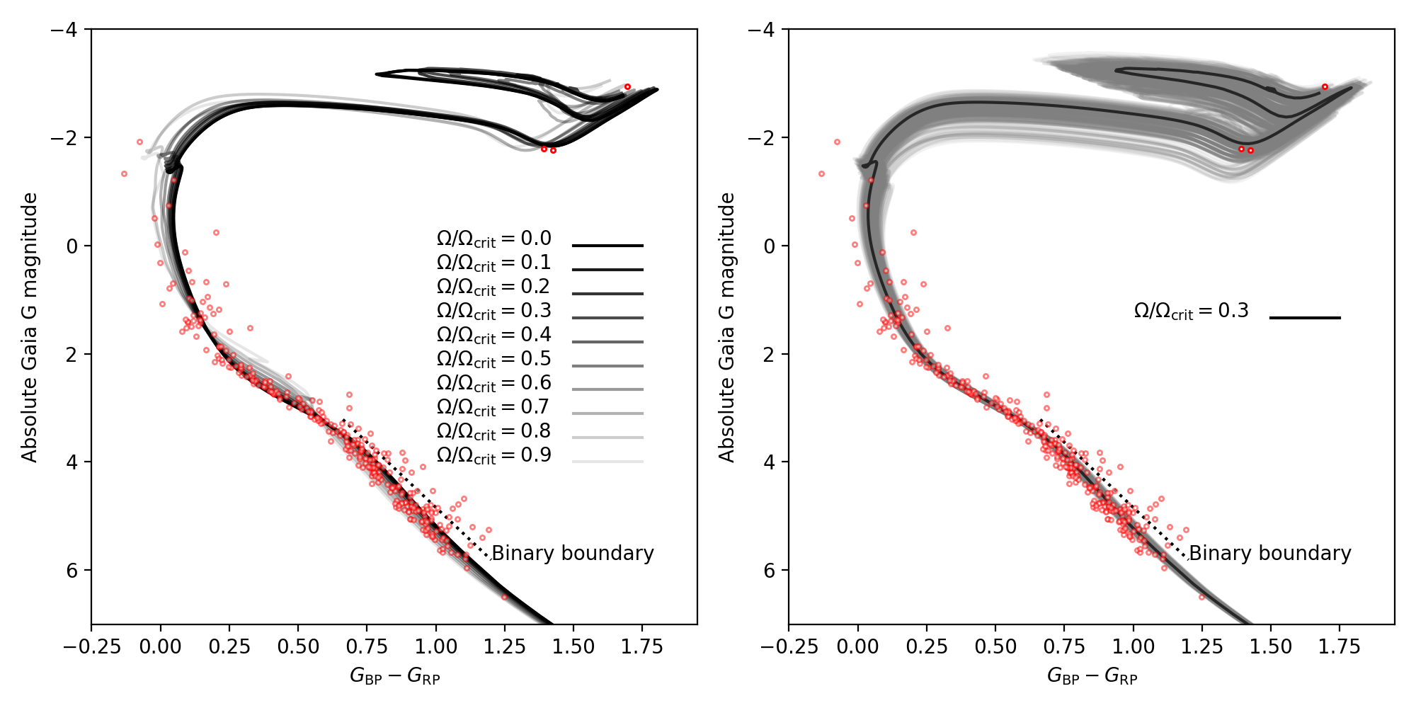
Figure 1: Observed Gaia DR3 CMD of NGC 2516. Left panel: fits for isochrones with varying rotation rates. Isochrones with $\Omega/\Omega_{\mathrm{crit}}\leq 0.4$ effectively reproduce the observed data. Right panel: the solid black isochrone represents the best-fitting result and $\Omega/\Omega_{\mathrm{crit}}=0.3$. The grey background tracks collectively represent the uncertainty, which is determined using a set of 500 isochrones randomly selected during a Monte-Carlo approach as explained in the text. The dotted line marks the boundary of the binary sequence.

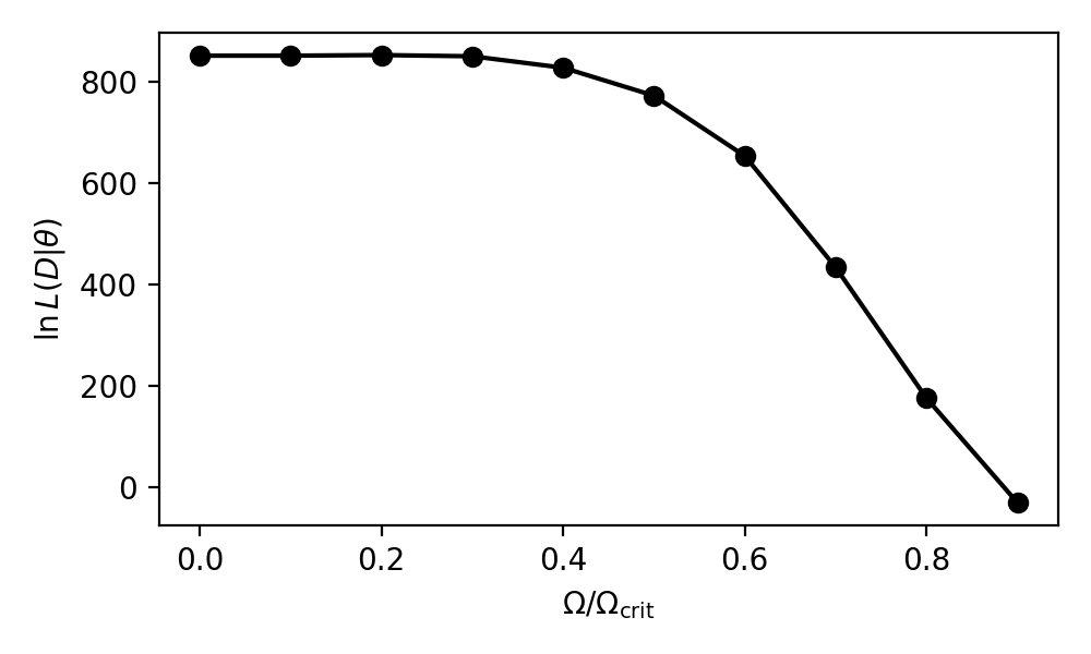
Figure 2: Relation between the log of the likelihood function (eq. 2 of the best-fitting isochrone and rotation rates $\Omega/\Omega_{\mathrm{crit}}$. Isochrones with $\Omega/\Omega_{\mathrm{crit}}>0.5$ show significantly small likelihood values, implying worse fitting to the observational data.

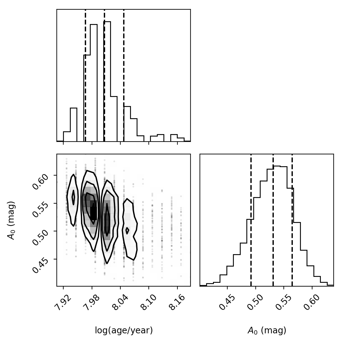
Figure 3: Posterior distributions of the isochrone fitting.

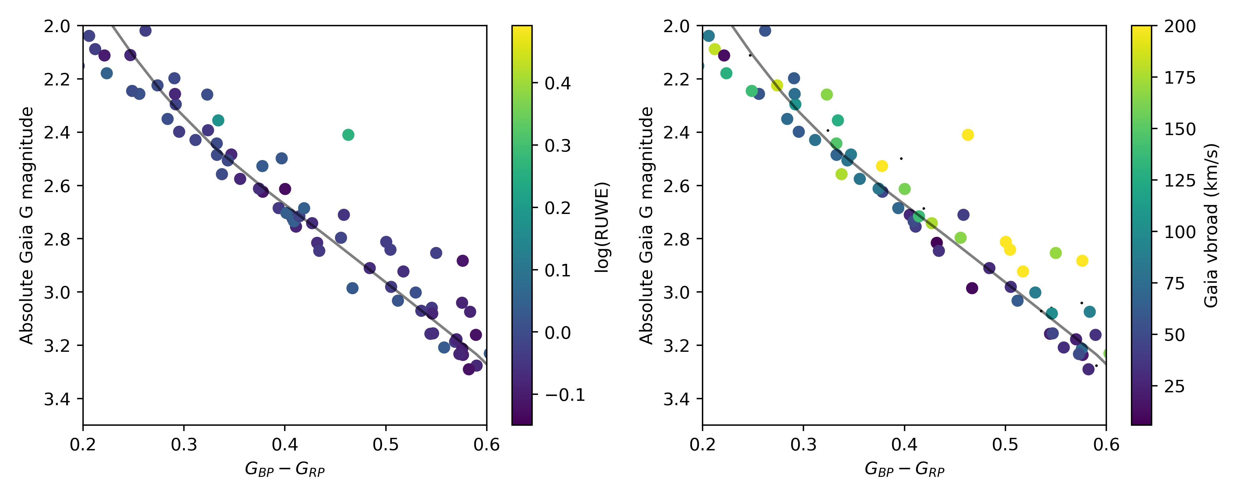
Figure 4: Zoom-in view of the CMD of NGC 2516 showing how binarity and rotation lead a star deviating from the main sequence. The ranges of the x- and y-axes are: $0.2\,\mathrm{mag}<G_{BP}-G_{RP}<0.6\,\mathrm{mag}$ and $2.0\,\mathrm{mag}<M_{G}<3.5\,\mathrm{mag}$. The stars are color-coded by RUWE (showing binarity) and line broadening (representing rotation rates), respectively. The small black dots are stars without broadening values in the Gaia DR3 database.

Recent studies have examined how rotation affects stellar evolution and consequently the isochrones (e.g. Paxton et al., 2019; Gossage et al., 2019). Therefore, we aim to identify the best-fitting isochrone for NGC 2516, and from it, derive the age and extinction of the cluster to more effectively consider the effects of rotation. we used MIST isochrones (MESA Isochrones and Stellar Tracks, Choi et al., 2016; Dotter, 2016) to fit our data. These are based on the Modules for Experiments in Stellar Astrophysics (MESA) code (version v7503, Paxton et al., 2011, 2013, 2015, 2018). The original MIST isochrones only include two rotation rates, specifically $\Omega/\Omega_{\mathrm{crit}}=0.0$ and $0.4$, where $\Omega_{\mathrm{crit}}$ represents the critical rotation at which the centrifugal force equals gravity at the equator of the isobar (Paxton et al., 2019). However, our objective is to comprehensively account for the impact of rotation. Therefore, we have explored isochrones encompassing a whole range of rotation rates, ranging from 0.0 to 0.9 $\Omega/\Omega_{\mathrm{crit}}$, with a step of 0.1 (Gossage et al., 2019). The physical processes related to rotation applied in the isochrone computations are done for the shellular approximation (Kippenhahn & Thomas, 1970). The chemical and angular momentum transport induced by rotation is computed from the diffusion equations from (Endal & Sofia, 1978). Gravity darkening was included according to (Espinosa Lara & Rieutord, 2011) as implemented in Paxton et al. (2019). Given that the temperature and luminosity decrease due to the gravity darkening effect depend on the inclination of the rotation axis with respect to the line-of-sight, Gossage et al. (2019) calculated the isochrones at a range of inclination angles and randomly sampled from them to create synthetic stellar populations. The isochrones used in this work represent an effect of gravity darkening averaged over inclination angles. Therefore, the scatter resulting from the gravity-darkening effect on the CMD should be distributed randomly around the best-fitting isochrone, rather than being concentrated on one side.

Due to the presence of main-sequence turn-offs and post-main-sequence stars, the shape of isochrones is rather intricate, that is, one colour index corresponds to multiple absolute magnitudes. Consequently, traditional least-squares fitting is not applicable here. Therefore, we consider an alternative fitting approach. We hypothesise that each observed data point follows a two-dimensional Gaussian distribution (without correlation) around the best-fitting point:

$$P(C,G)=\frac{1}{2\pi\sigma_{C}\sigma_{G}}\exp\left(-\frac{1}{2}\left[\left(\frac{C-C_{\mathrm{model}}}{\sigma_{C}}\right)^{2}+\left(\frac{G-G_{\mathrm{model}}}{\sigma_{G}}\right)^{2}\right]\right),$$ (1)

where $C$ is the Gaia colour index $G_{\mathrm{BP}}-G_{\mathrm{RP}}$, and G is the absolute Gaia G band magnitude with extinction. $C_{\mathrm{model}}$ and $G_{\mathrm{model}}$ are the colour index and absolute magnitude of the closest point in the isochrone after extinction correction, while $\sigma_{C}$ and $\sigma_{G}$ are the standard deviations of the colour index and of the absolute G band magnitude. We interpolate the isochrones, inserting ten values between each pair of adjacent points, to calculate the theoretically predicted points closest to a given observed point. The observed $\sigma_{C}$ and $\sigma_{G}$ values obtained from Gaia are notably smaller than the scatter observed in the CMD. This discrepancy could potentially be attributed to uncertainties in input physics, including poor calibration of internal mixing, variations in inclinations, differential extinction, various initial rotation rates, and unknown physical causes of the eMSTO. Therefore, we have opted to use significantly larger values for $\sigma_{C}$ and $\sigma_{G}$ instead of the Gaia’s observation uncertainties to represent the residual’s standard deviations. By calculating a fourth-degree polynomial fit between the absolute magnitude and the colour index, these values of the uncertainties are set to $\sigma_{C}=0.056\,\mathrm{mag}$ and $\sigma_{G}=0.332\,\mathrm{mag}$.

The final likelihood function is the product of a series of probabilities.

$$L(D|\theta)=\prod_{i}P(C_{i},G_{i}),$$ (2)

where $D$ denotes the observed data, $C_{i}$ and $G_{i}$ are the colour index and absolute G magnitude of the $i^{\mathrm{th}}$ star, $\theta=\{\mathrm{log(age)},A_{0}\}$ is the vector of input parameters which contains the age and extinction at 550 nm. The input colour index and absolute magnitude derived from the MIST isochrones represent their intrinsic values, so we needed to calculate the values after extinction correction for the $G$, $G_{\mathrm{BP}}$, and $G_{\mathrm{RP}}$ bands. Specifically, we applied the extinction law as described by Danielski et al. (2018), which is calculated as

$$\begin{split}A_{m}/A_{0}&=a_{1}+a_{2}X+a_{3}X^{2}+A_{4}X^{3}+a_{5}A_{0}+a_{6}A_{0}^{2}+a_{7}A_{0}^{3}\\ &+A_{8}A_{0}X+a_{9}A_{0}X^{2}+A_{10}XA_{0}^{2},\end{split}$$ (3)

where $A_{m}$ stands for the extinction in the G, BP, and RP bands, $A_{0}$ is the extinction at 550 nm, and $X$ is the intrinsic colour index $G_{\mathrm{BP}}-G_{\mathrm{RP}}$. The coefficients $a_{i}$ for the Gaia DR3 passband were given by Riello et al. (2021). Considering the positions of our stars on the HRD, we use the coefficients adapted for the upper regions of the HRD, which encompass giants and the upper segment of the main sequence, up to approximately $G\sim 5$ mag.

We find that the data points exhibit a large spread in the low-temperature area, where $G_{\mathrm{BP}}-G_{\mathrm{RP}}$ is approximately greater than 0.65 mag (in Fig.1). This spread is attributed to binarity. As a clear binary sequence is not visible, we have excluded the data points above the dotted line in Fig.1, which were manually determined to begin at ($G_{\mathrm{BP}}-G_{\mathrm{RP}}=0.6626,G=3.217$) and end at ($G_{\mathrm{BP}}-G_{\mathrm{RP}}=1.2011,G=5.810$).

A pre-search of the best-fitting model was done by calculating a coarse grid, using $7<\mathrm{log(age/yr)}<9$ with an evolution step of 0.02 and $0\,\mathrm{mag}<A_{0}<1\,\mathrm{mag}$ with step of 0.025 mag. After finding the initial best-fitting values of log(age) and $A_{0}$, we estimate their uncertainties using a Monte-Carlo approach. In each iteration, we added a Gaussian random noise perturbation to the original data using $\sigma_{C}$ and $\sigma_{G}$, and searched for the best-fitting model in a fine grid by calculating the likelihood values. The parameter spaces are: ages within the first eight and last eight steps of the initial age range, and extinction within a range of 0.1 mag before and after the initial extinction, with a step size of 0.01 mag. The age and $A_{0}$ corresponding to the largest likelihood in each iteration were recorded, and their uncertainties were calculated after 1000 iterations.

Figure 1 illustrates the best-fitting isochrones. In the left panel, we find that the isochrones with $\Omega/\Omega_{\mathrm{crit}}\leq 0.4$ successfully reproduce the observed CMD, while those with $\Omega/\Omega_{\mathrm{crit}}\geq 0.5$ exhibit discrepancies from the observations. Additionally, as shown in Fig. 2, isochrones within $\Omega/\Omega_{\mathrm{crit}}\leq 0.4$ yield similar maximum likelihood values, but the likelihood begins to decrease rapidly when $\Omega/\Omega_{\mathrm{crit}}\geq 0.5$. Obviously, not all stars in the cluster will have been born with the same value of $\Omega/\Omega_{\mathrm{crit}}$. All the isochrones with $\Omega/\Omega_{\mathrm{crit}}\leq 0.4$ produce satisfactory results in the CMD.

The right panel of Fig. 1 presents one of the best-fitting outcomes, featuring $\Omega/\Omega_{\mathrm{crit}}=0.3$ for all stars simultaneously. Under this premise, the grey background represents the uncertainty range obtained from randomly selected 500 isochrones from the iterations with $\Omega/\Omega_{\mathrm{crit}}\leq 0.4$. The presence of the three post-main-sequence stars imposes additional constraints on isochrone age, yet considerable spread persists in the post-main-sequence phases. Finally, under equal weighting of the isochrone fitting with $\Omega/\Omega_{\mathrm{crit}}\leq 0.4$, we derived $\mathrm{log(age/year)=8.01\pm 0.06}$ (equivalent to $102\pm 15$ Myr) and an extinction value of $A_{0}=0.53\pm 0.04\,\mathrm{mag}$. The posterior distributions are shown in Fig. 3. Our determined age for NGC 2516 is somewhat younger than that of the Pleiades, opposite to the prior study using gyrochronology (Fritzewski et al., 2020). The age discrepancy might arise from different approaches. Applying the same isochrone-fitting approach to both NGC 2516 and the Pleiades could still yield a similar age for both open clusters.

Regarding the extinction, $A_{0}=0.53\,\mathrm{mag}$ lead to a reddening of 0.25 mag given a intrinsic Gaia colour index $\left(G_{\mathrm{BP}}-G_{\mathrm{RP}}\right)_{0}=0.2\,\mathrm{mag}$. If we assume $A_{0}\approx A_{V}$ and $A_{V}=3.1E(B-V)$, where $A_{V}$ represents extinction at the V band, we obtained a reddening value of $E(B-V)\approx 0.17\,\mathrm{mag}$. Alternatively, using equation 3 and the extinction coefficients from Casagrande & VandenBerg (2018), which state that $E(\mathrm{BP}-\mathrm{RP})=(3.374-2.035)E(B-V)$, we obtain a similar reddening value of $E(B-V)\approx 0.18\,\mathrm{mag}$. It is worth noting that this reddening value is slightly higher than the one reported in a previous study ($0.112\pm 0.024\,\mathrm{mag}$) by Sung et al. (2002). Additionally, the Gaia total galactic extinction map provides an average extinction value of $A_{0}=0.4358\,\mathrm{mag}$ within a radius of 0.25’. Even after transforming this value to $E(B-V)$ (which is 0.14 mag), it remains slightly higher than the literature value reported by Sung et al. (2002).

We also investigate the impact of different extinction values on age determination. We find that the values suggested by Sung et al. (2002) and those from the Gaia total galactic extinction map both lead to the same age estimate of $\log(\mathrm{age/yr})=7.99$. This estimate is just one step before our best-fitting age and still falls within the uncertainty range. Therefore, it appears that extinction does not significantly change the age determination.

Figure 4 displays a zoom-in of the CMD, which roughly corresponds to the region of the classical instability strip. In the left panel, we can observe that Gaia’s RUWE binary indicator values (see definition in Gaia Collaboration et al., 2023b) show little variation in this region, making it difficult to distinguish binary systems based solely on RUWE values. Only one star exhibits a significantly higher RUWE value, and interestingly, this star happens to fall to the right of the best-fit isochrone. In the right panel, we colour-coded the points with the Gaia vbroad parameter (see definition in Frémat et al., 2023a), revealing that many stars have high vbroad values (greater than 200 km s^-1). These stars tend to be located on the right of the best-fitting isochrone, indicating the influence of gravity darkening caused by fast rotation and the flattening it induces (Pérez Hernández et al., 1999).

4 Light curve reduction and variability identification

4.1 Light curve reduction

The unique advantage of NGC 2516 is its location near the edge of the southern continuous viewing zone of the TESS satellite. Consequently, TESS offers nearly continuous observations spanning 11 sectors, for a total of approximately 297 days. Our analysis used the data from Cycle 1 and Cycle 3, encompassing sectors 1, 4, and 7 to 11, as well as sectors 27, 31, and 34 to 37. A one-year gap is seen during Cycle 2 when the TESS satellite observed the northern celestial hemisphere. In Cycle 1, observations were taken at a cadence of 30 minutes, whereas in Cycle 3, the cadence was reduced to 10 minutes.

We used the asteroseismic reduction pipeline developed by Garcia et al. (2022b) to download and process the TESS photometric data. The TESS Full Frame Images were obtained from the Mikulski Archive for Space Telescope (MAST) using the TESScut API (Brasseur et al., 2019). For each star, a cutout of size 25 pixels $\times$ 25 pixels was applied. This size allows for the examination of neighbouring stars, and assessment of contamination, and provides an adequate number of background pixels for subtraction.

Flux extraction using custom apertures was performed using the Python package Lightkurve (Lightkurve Collaboration et al., 2018a). While the apertures in the pipeline by Garcia et al. (2022b) were optimised to mitigate severe contamination, it is challenging to completely avoid contamination in the crowded NGC 2516 field. For stars significantly affected by contamination, we employed aperture radii smaller than those automatically determined by the code. We calculated contamination levels by fitting Gaussian profiles of the target star and nearby stars. A star was excluded from the analysis if the contaminated flux constituted more than 10% of the total flux. After excluding the contaminated stars, our sample contains 301 of stars for further analysis. Subsequently, detrending was performed on a sector-by-sector basis, involving background subtraction and principal component analysis.

After obtaining the light curves, we calculated their Fourier transform to identify their light variability. The Lomb-Scargle algorithm was used for our stars to calculate their amplitude spectra (Lomb, 1976; Scargle, 1982), which is suitable for unevenly spaced data.

4.2 Variable star classification

We identified three red giant stars in the cluster, while all the other stars are main-sequence stars. Therefore, we primarily focus on the types of variables that occur among main-sequence stars, namely p-mode pulsators (mainly $\delta$ Sct stars), g-mode pulsators ($\gamma$ Dor and SPB stars), stars with surface modulation, and eclipsing binaries. The g-mode and p-mode pulsators typically exhibit numerous narrow frequency peaks within their respective frequency regimes. The frequencies of p-mode pulsations are generally above $\sim$10 $\mathrm{d^{-1}}$, while g-mode pulsations have frequencies below $\sim$5 $\mathrm{d^{-1}}$. Eclipsing binaries often exhibit a fundamental frequency along with a series of harmonics in their power spectra. These distinct features aid us in identifying various types of variable stars. Rotational modulation occurs along the main sequence, notably in cool stars subject to magnetic braking and in hotter counterparts revealing chemical or temperature spots. Specifically, we search for a hump in the low-frequency range caused by the rotational frequency and differing from additional narrow frequency peaks due to pulsations, and we also require the presence of harmonics of the rotational frequency.

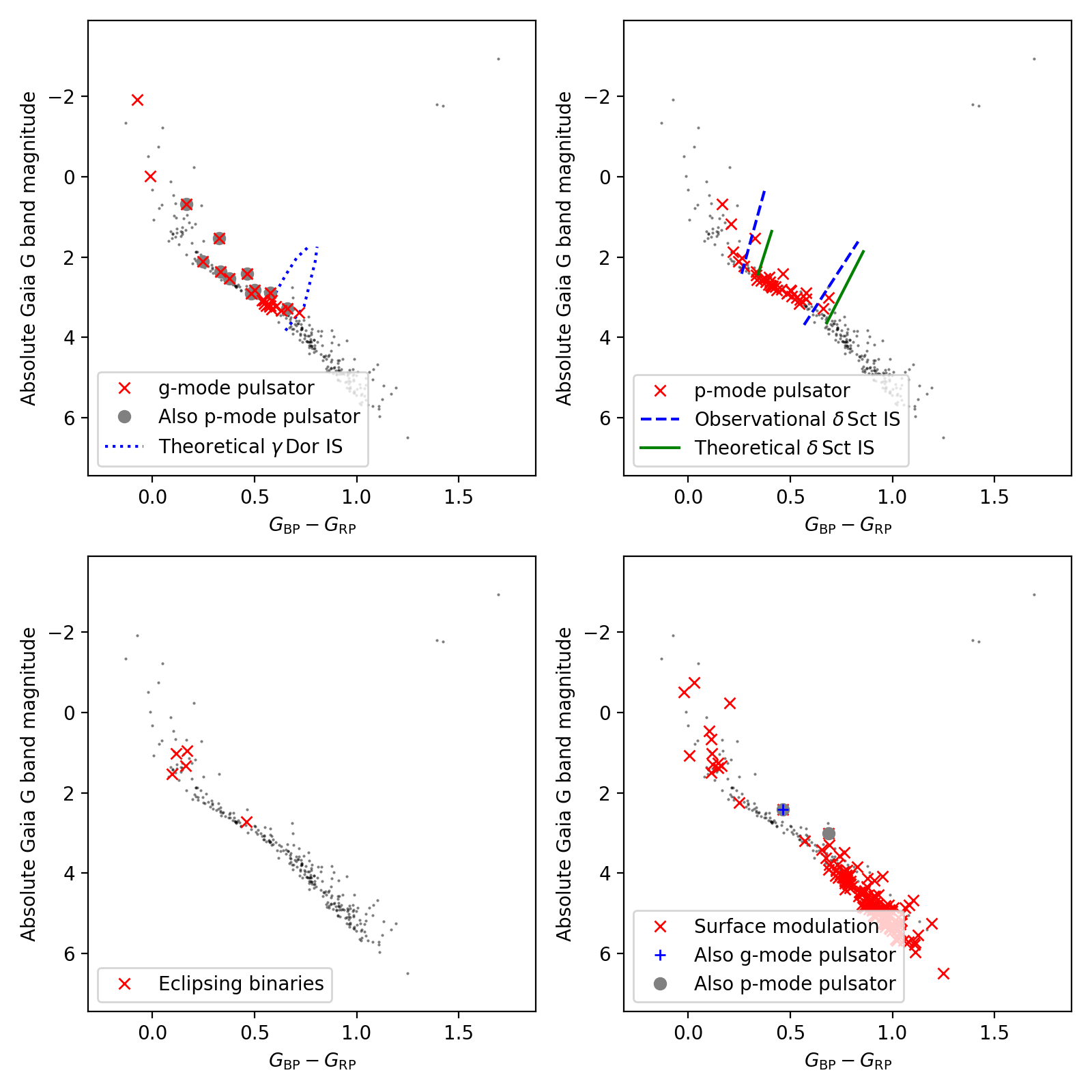
Figure 5: Locations of variable stars on the CMD of NGC 2516.

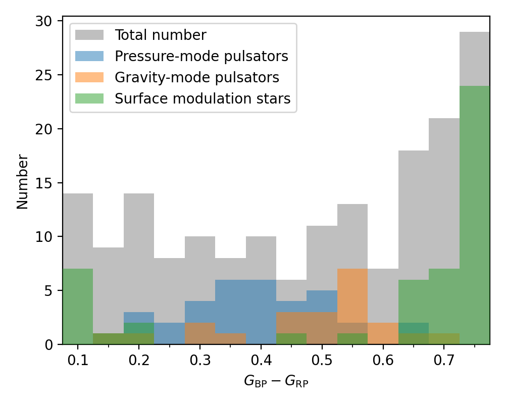
Figure 6: Histogram of the numbers of the p-mode pulsator, g-mode pulsator, surface modulations, and the total star in our sample. The bin size of the colour index $G_{\mathrm{BP}}-G_{\mathrm{RP}}$ is 0.05. Pulsating stars (p- and g-mode pulsators) have high fractions around $G_{\mathrm{BP}}-G_{\mathrm{RP}}$ of 0.5 mag while surface modulation stars appear with small or large $G_{\mathrm{BP}}-G_{\mathrm{RP}}$.

We find 24 g-mode pulsators, 35 p-mode pulsators, 5 eclipsing binaries, and 147 surface modulation stars. Figure 5 illustrates the positions of these variables in the Gaia DR3 CMD of NGC 2516. For isolated stars, determining the positions of variable stars on the HRD and evolutionary stages remains challenging due to various factors, including extinction, inaccurate temperature and luminosity measurements, or large uncertainty on mass. Consequently, defining the observational instability strip (IS) of the variables in the cluster is non-trivial. The CMD of a cluster offers a better opportunity to investigate the instability strips of variable stars, as their locations and parameters are well-defined in the CMD.

In the case of g-mode pulsators (shown in the upper left panel of Fig. 5), we observe a group of stars within a range of $G_{\mathrm{BP}}-G_{\mathrm{RP}}$ values from approximately 0.4 mag to 0.6 mag, which is identified as the IS of $\gamma$ Dor stars. We plotted the theoretical IS by Dupret et al. (2005) after transforming the effective temperature and luminosity to the observed Gaia colour index $G_{\mathrm{BP}}-G_{\mathrm{RP}}$ and absolute G band magnitude with extinction. We find that the theoretical IS is slightly redder than the dense area of g-mode pulsators, and many g-mode pulsators appear above the blue edge of the theoretical IS. In Fig. 6, we show the histograms as a function of colour index for the various classes of pulsators. The distribution peaks around 0.5 mag for the observed $\gamma$ Dor IS. In this region, about 50% of stars show g-mode pulsations.

The upper right panel of Fig. 5 depicts the distribution of p-mode pulsators. We observe that p-mode pulsators are present within the $G_{\mathrm{BP}}-G_{\mathrm{RP}}$ range of approximately 0.2 mag to 0.6 mag. These stars are classified as $\delta$ Sct stars, as their temperatures do not reach the range of $\beta$ Cep stars. The observed IS of $\delta$ Sct stars in the cluster is broader than that of the $\gamma$ Dor stars. We find that the observed $\delta$ Sct IS by Murphy et al. (2019) matches the observation, while the theoretical IS by Dupret et al. (2005) is still slightly redder than the observations. Examining Fig. 6, we note that $\delta$ Sct stars dominate the IS. Approximately 60% to 80% of the stars within the IS are identified as $\delta$ Sct stars. This fraction is consistent with the findings of a previous study conducted on the Pleiades cluster (Bedding et al., 2023). The fraction slightly exceeds the value found for the Kepler field (Murphy et al., 2019), which may be due to the age difference.

In the lower-left panel of Fig. 5, we observe the positions of eclipsing binaries on the CMD. The majority of these binaries appear to lie near the main-sequence turn-off. This observation is consistent with the nature that high-mass stars tend to exhibit a higher binary fraction (Moe & Di Stefano, 2017). In table 1, we listed the TIC number, Gaia colour index, and the orbital period for each eclipsing binary. The orbital period was measured using the procedure described in (Li et al., 2020a), which is mainly based on the $\mathrm{O}-\mathrm{C}$ (O minus C) method (Sterken, 2005). We find that TIC 382529041 shows a variation in eclipse depths. Its $\mathrm{O}-\mathrm{C}$ diagram reveals a long-period third-component gravity perturbation with an estimated very high eccentricity.

Table 1: 5 eclipsing binaries in NGC 2516.

TIC	$G_{\mathrm{BP}}-G_{\mathrm{RP}}$	$P_{\mathrm{orb}}$ (d)
341793209	0.458	0.28233919(23)
372913337	0.17	1.786037(8)
372913472	0.161	0.30749301(13)
382529041	0.115	0.3475920(13)
410451083	0.094	0.8593202(12)

The stars exhibiting surface modulation are situated in the lower right panel of Fig. 5. It is evident that there exists a distinct gap wherein very few stars with surface modulations are observed, ranging from $G_{\mathrm{BP}}-G_{\mathrm{RP}}\sim 0.2$ mag to approximately 0.6 mag. This is the region predominantly occupied by $\delta$ Sct and $\gamma$ Dor stars. This gap is also evident in the green histogram displayed in Fig.6. We observe a considerably higher fraction of cool stars displaying surface modulation with $G_{\mathrm{BP}}-G_{\mathrm{RP}}>0.6$ mag. This occurrence is attributed to low-mass stars with a convective envelope, resulting in surface activity. Furthermore, some stars located at the MSTO also show surface modulation in the presence of fast rotation close to the critical rate.

4.3 Gravity-mode pulsators

Table 2: TAR fitting results of the 11 g-mode pulsators in NGC 2516.

TIC	$f_{\mathrm{rot}}$ ($\mathrm{d^{-1}}$)	$\Pi_{0}$ (s)
281582674	$3.11_{-0.08}^{+0.05}$	$6500_{-1000}^{+800}$
308307454	$1.051_{-0.009}^{+0.010}$	$4730_{-60}^{+60}$
308992761	$2.94_{-0.19}^{+0.12}$	$4600_{-1300}^{+1300}$
341043961	$3.01_{-0.08}^{+0.08}$	$5000_{-700}^{+800}$
358466708	$1.338_{-0.027}^{+0.023}$	$9400_{-900}^{+900}$
358466729	$2.130_{-0.014}^{+0.014}$	$4400_{-300}^{+400}$
364398040	$2.94_{-0.05}^{+0.04}$	$4800_{-400}^{+400}$
372912679	$3.00_{-0.08}^{+0.07}$	$4800_{-600}^{+700}$
372913043	$2.98_{-0.06}^{+0.05}$	$4900_{-600}^{+500}$
410451583	$2.96_{-0.10}^{+0.09}$	$5100_{-900}^{+1100}$
410452218	$2.80_{-0.06}^{+0.05}$	$4800_{-500}^{+500}$

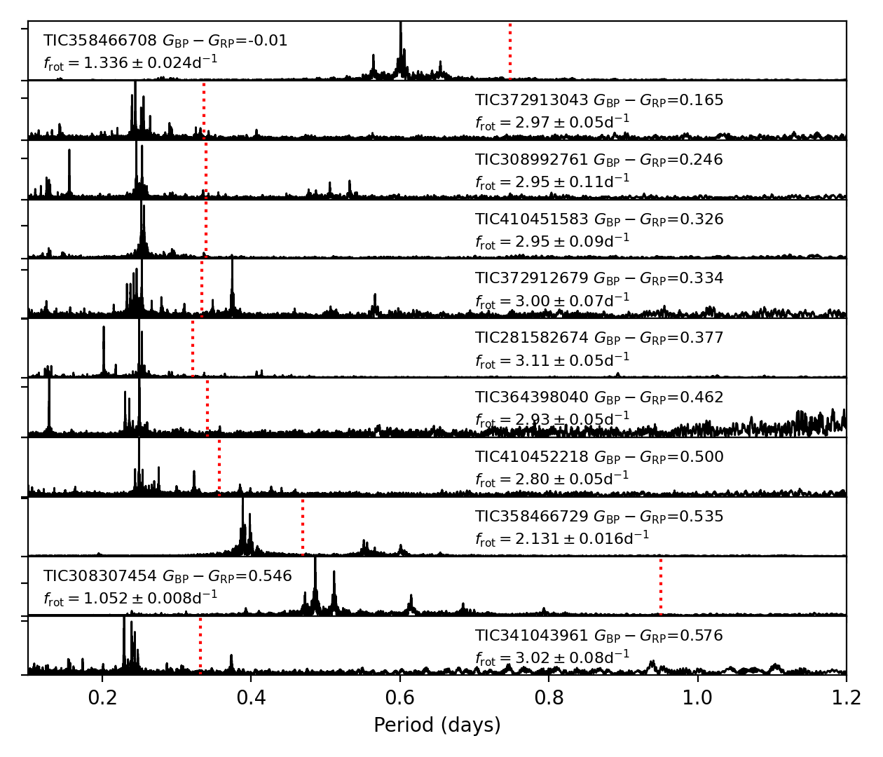
Figure 7: 11 g-mode pulsators with clear period spacing patterns, sorted in descending order by their Gaia colour index $G_{\mathrm{BP}}-G_{\mathrm{RP}}$ from top to bottom. The red vertical lines mark their near-core rotation periods derived from the modes by adopting the TAR.

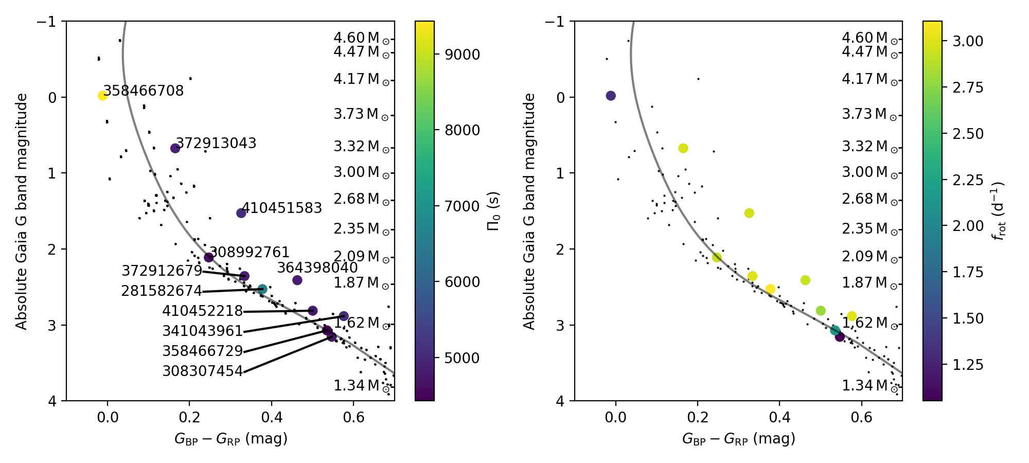
Figure 8: Location of $\gamma$ Dor stars on the CMD with the best-fitting isochrone. The large circles show the $\gamma$ Dor stars with clear period spacings, colour-coded by their buoyancy travel time (left panel) or near-core rotation rates (right panel). The black dots are the other cluster members and the grey solid line is the best-fitting isochrone. We also indicate the masses of the models on the right edges of each panel. In the left panel, we show the TIC numbers of the stars.

Not all of the 24 g-mode pulsators allow for mode identification, because only some of them show clear period spacing patterns. Period-spacing search algorithms for $\gamma$ Dor stars were developed by Van Reeth et al. (2015b) and Christophe et al. (2018). Here, we search for and identify such spacing patterns following the procedure by Li et al. (2019c). It previously yielded hundreds of $\gamma$ Dor stars in the Kepler field, including $\gamma\,$Dor stars in eclipsing binaries (Li et al., 2020b, 2019d, a). A similar method to search for the period spacing patterns was developed by Garcia et al. (2022b) and yielded tens of $\gamma$ Dor field stars in the TESS continuous viewing zone Garcia et al. (2022a).

We find 11 g-mode stars exhibiting clear period spacing patterns. We measured their asymptotic spacings and near-core rotation rates following the framework by Van Reeth et al. (2016), which relies on the traditional approximation of rotation (TAR). With the influence of rotation, the period spacing for g modes is no longer constant. Rather, the g-mode periods in the co-rotating frame can be rewritten as

$$P_{nlm,\mathrm{co}}=\frac{\Pi_{0}}{\sqrt{\lambda_{l,m,s}}}\left(n+\alpha_{\mathrm{g}}\right).$$ (4)

In this equation, $\Pi_{0}$ is the asymptotic spacing representing the travel time of the waves within their mode cavity determined by the buoyancy frequency and is hence called the buoyancy travel time (Aerts, 2021), $s=2f_{\mathrm{rot}}/f_{\mathrm{co}}$ is the spin parameter as a function of the rotation frequency $f_{\mathrm{rot}}$ and pulsation frequency in the co-rotating frame $f_{\mathrm{co}}$, $\lambda$ is the eigenvalue of the Laplace tidal equation, which can be computed with the gyre code (Townsend & Teitler, 2013; Townsend et al., 2018), $\alpha_{\mathrm{g}}$ is a phase term, and $n,l,m$ are the quantum numbers of the mode. All the period spacing patterns and the TAR fitting results are shown in Sect. B.

Figure 7 displays all the 11 g-mode pulsators with clear period spacing patterns. We observe a distinct orderliness in the amplitude spectra of these stars within the same star cluster after sorting them by Gaia colour index. We find that with colour index between 0.5 mag and 0.165 mag, those stars show similar near-core rotation rates, which is about 3 $\mathrm{d^{-1}}$. The dominant mode frequencies at about 0.25 d are identified as $l=1$, $m=1$ g modes subject to the Coriolis acceleration and projected into the line-of-sight with value $f_{\mathrm{rot}}$. Additionally, another group of frequencies is observed at a period of approximately 0.13 d, corresponding to $l=2$, $m=2$ g modes shifted by $2f_{\mathrm{rot}}$ towards the observer’s reference frame.

We present the results of asymptotic spacing $\Pi_{0}$ and near-core rotation frequency $f_{\mathrm{rot}}$ in Fig. 8 and Table 2. In the left panel of Fig. 8, we observe that the majority of our g-mode pulsators have $\Pi_{0}$ around 5000 s. This value is typical for $\gamma$ Dor stars, although it is somewhat higher than the average value of the $\gamma$ Dor field stars derived from Kepler and TESS data (which is 4000 s, as reported in Li et al., 2020b; Garcia et al., 2022a). The value of $\Pi_{0}$ is correlated with the central hydrogen abundance, along with other key quantities describing the internal mixing, as well as the initial chemical composition (Mombarg et al., 2019; Ouazzani et al., 2019). Hence it provides an estimation of the stellar age, provided that the level of internal mixing can be deduced and that the metallicity of the star is known. Here, we assume all the cluster members were born with the same initial metallicity. Consequently, the higher value of $\Pi_{0}$ can be attributed to the young age of the cluster. It is worth noting that $\Pi_{0}$ remains relatively consistent for all pulsators within the $G_{\mathrm{BP}}-G_{\mathrm{RP}}$ range of 0.2 mag to 0.6 mag, indicating a limited sensitivity to (core) mass. TIC 358466708 exhibits a value of $\Pi_{0}\approx 9400$ s, which is significantly higher than the typical value for $\gamma$ Dor stars but is typical for SPB stars (Pedersen et al., 2021). Additionally, the high temperature of this star ($12070\pm 170\,\mathrm{K}$) confirms its SPB nature. TIC 372913043 is also a SPB star with temperature of $11510\pm 240\,\mathrm{K}$. Their temperatures were measured using the high-resolution spectra, as discussed in Sect. 5.

We show the near-core rotation rates in the right panel of Fig. 8 and find a clear correlation with colour index. The near-core rotation rates increase from about 1 $\mathrm{d^{-1}}$ at $G_{\mathrm{BP}}-G_{\mathrm{RP}}\approx 0.6\,\mathrm{mag}$ to 3 $\mathrm{d^{-1}}$. However, the SPB star TIC 358466708 shows a relatively slow rotation, back to $1\,\mathrm{d^{-1}}$. This is in agreement with the findings for Kepler fields stars, where the SPB stars are on average slower rotators than the $\gamma\,$Dor stars (Aerts, 2021, see their Fig. 6). The rotation rates of the $\gamma$ Dor stars in NGC 2516 are significantly higher than those obtained from the Kepler and TESS data (Li et al., 2020b; Garcia et al., 2022a), where the median rotation rate is approximately $1\,\mathrm{d^{-1}}$. The faster rotation that we find here for the cluster stars is due to their younger age compared to those of field stars (Mombarg et al., 2021).

Additionally, we identify two g-mode pulsators (TIC 358466708 and TIC 372913043) located at the MSTO, which are categorised as SPB stars. The effective temperatures measured by the spectra in Sect. 5 further confirm the classification of SPB stars. TIC 372913043 is somewhat suspicious, as it exhibits a small asymptotic spacing value ($4900^{+500}_{-600}\,\mathrm{s}$, Table 2), which should be within the typical range for $\gamma$ Dor stars. We investigated the possibility of contamination and found the contamination level to be 1.8%, indicating that 1.8% of the flux in the aperture comes from other sources. There is only one star that could potentially contaminate the target, which is also a cluster member (TIC 372913044, with apparent Gaia G band magnitude of 12.84 mag). As a comparison, TIC 372913043 has a magnitude of 8.74 mag, 4.1 mag brighter than the neighbour star. However, given its low colour index ($G_{\mathrm{BP}}-G_{\mathrm{RP}}=0.92\,\mathrm{mag}$, corresponding to $T_{\mathrm{eff}}<5830\,\mathrm{K}$), the neighbouring star TIC 372913044 is unlikely to exhibit g-mode period spacings. Therefore, we ruled out contamination as a cause. The reason for the small asymptotic spacing in this SPB star is likely due to evolution: as seen in Fig. 8, TIC 372913043 is located in the eMSTO and is departing the main sequence, which means its asymptotic spacing should be decreasing rapidly.

We also identify some g-mode pulsators situated between the SPB and $\gamma$ Dor strips. This is fully in line with the findings by Gaia Collaboration et al. (2023a) from Gaia DR3 light curves and points to fast rotators with g modes Aerts et al. (2023).

4.4 Pressure-mode pulsators

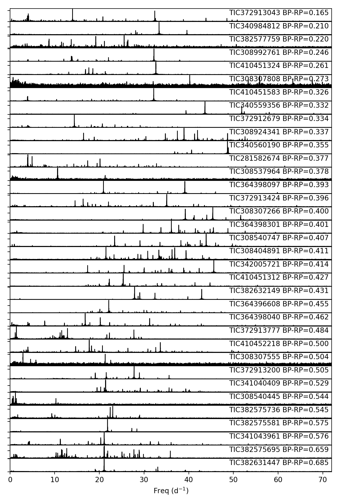
Figure 9: Amplitude spectra of the $\delta$ Sct stars in NGC 2516, sorted by colour index. The top panel has the star with the smallest colour index hence the highest effective temperature.

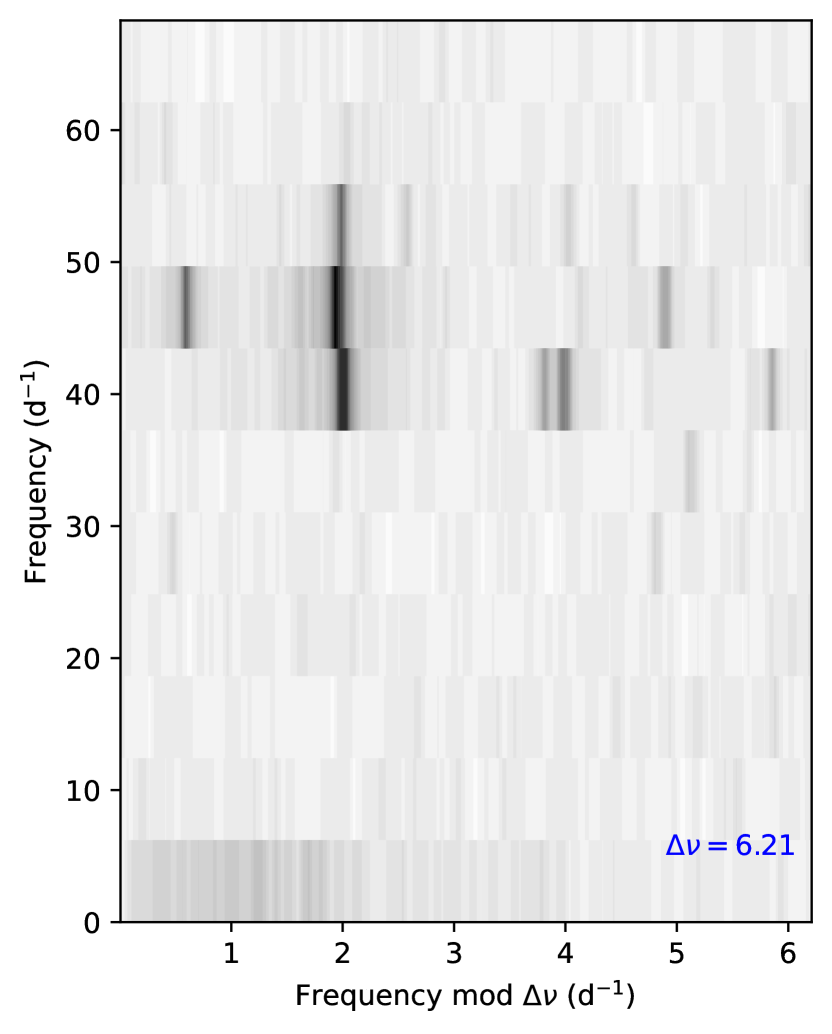
Figure 10: Echelle diagram of the $\delta$ Sct star TIC 308307266. A frequency separation is seen with $\Delta\nu\approx 6.21\,\mathrm{d^{-1}}$.

The mode identification of $\delta$ Sct stars is a long-standing question, and leads to difficulty in asteroseismic exploitation of their internal physical properties (Bedding et al., 2020). We show all the amplitude spectra of the $\delta$ Sct stars in NGC 2516, sorted by their colour index, in Fig. 9. We find that their amplitude spectra are well-ordered as a function of colour index. For the low-temperature stars ($G_{\mathrm{BP}}-G_{\mathrm{RP}}>0.411$ mag, the bottom part of Fig. 9), a series of strong frequency peaks appear near $21\,\mathrm{d^{-1}}$, which is identified as the radial fundamental mode frequency (Bedding et al., 2020). In the $G_{\mathrm{BP}}-G_{\mathrm{RP}}$ region from 0.5 mag to 0.4 mag (middle part of Fig. 9), we find a relation between the mean pulsation frequency and temperature. With increasing temperature, the envelope of the pulsation frequencies moves to higher frequency (Balona & Dziembowski, 2011; Barceló Forteza et al., 2018; Bowman & Kurtz, 2018; Barceló Forteza et al., 2020; Hasanzadeh et al., 2021). Finally, for the hotter stars (with $G_{\mathrm{BP}}-G_{\mathrm{RP}}\leq 0.396$ mag), another series of strong peaks aligns at frequency around $33\,\mathrm{d^{-1}}$, which we interpret as the signature of second overtone radial modes given their factor $\sim\!0.64$ shorter period than those of the fundamental modes (e.g. Netzel et al., 2022).

We attempted to identify regular frequency separations among these $\delta$ Sct stars. In Fig. 10, the échelle diagram of TIC 308307266 displays a ridge corresponding to $l=1$ modes with four distinct peaks separated by a large frequency spacing of $\Delta\nu\approx 6.21\,\mathrm{d^{-1}}$, roughly in agreement with mean stellar densities of $\delta\,$Sct stars if we keep in mind that $\Delta\nu$ is affected by fast rotation. We did not observe a corresponding ridge for its $l=0$ modes, but this is not so surprising given that such ridges due to radial modes tend to be strongly blended while those of the dipole modes are not, making the latter easier to find (Bedding et al., 2020). No other $\delta\,$Sct star in the cluster was found to reveal a clear large frequency separation.

4.5 Oscillations of the cluster giants

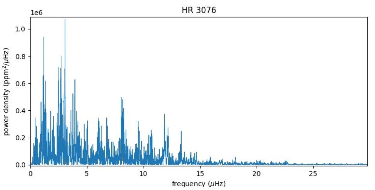
Figure 11: Power density spectra of the red giant HR 3036.

There are three red giants in NGC 2516: HR 3076 (TIC 382510863; HD 64320; $G=6.34$), SAO 250043 (TIC 372913375; $G=6.30$) and HD 65662 (TIC 358466601; $g=5.18$). We used the SPOC 2-minute light curves to search for solar-like oscillations. To measure $\nu_{\rm max}$, we used the nuSYD method described by Sreenivas et al. (submitted to MNRAS). We note that the nuSYD solar value of $\nu_{\rm max}$ is 3154 $\mu$Hzİn HR 3076, we found a very clear detection with $\mbox{$\nu_{\rm max}$}=10.8\pm 0.3\,\mbox{$\mu$Hz}$ and $\mbox{$\Delta\nu$}=1.27\pm 0.02\,\mbox{$\mu$Hz}$. In the other two stars, the oscillations were not so clear but the likely values of $\nu_{\rm max}$ are $12.5\pm 0.5\,\mbox{$\mu$Hz}$ for SAO 250043 and $2.6\pm 0.3\,\mbox{$\mu$Hz}$ for HD 65662. We were not able to identify $\Delta\nu$ for these two stars.

For HR 3036, we have both $\nu_{\rm max}$ and $\Delta\nu$ and so we used the standard asteroseismic scaling relations (e.g., Jackiewicz, 2021) to calculate the mass. Using $\mbox{$T_{\rm eff}$}=4704\pm 122$ K from Stassun et al. (2019) gives a mass of $3.8\pm 0.5\,\mbox{$\text{M}_{\odot}$}$. Without a value of $\Delta\nu$, we can still use $\nu_{\rm max}$ to estimate a mass by using the Gaia luminosity. We calculated the luminosities of the stars using the equation

$$-2.5\log L=G+BC-M_{\mathrm{bol,\odot}}-A_{G},$$ (5)

where $G$ is the absolute magnitude in the Gaia G band, $BC$ is the temperature-only dependent bolometric correction, $M_{\mathrm{bol,\odot}}=4.74$ is the solar absolute bolometric magnitude, and $A_{G}$ is the extinction in the Gaia G band given by the isochrone fitting in Sect. 3. The bolometric correction is calculated as

$$BC=\sum_{i=0}^{4}b_{i}\left(T_{\mathrm{eff}}-T_{\mathrm{eff,\odot}}\right)^{i},$$ (6)

with the coefficients $b_{i}$ given by Andrae et al. (2018). We used the effective temperatures $T_{\mathrm{eff}}$ given by Gaia to calculate the luminosities, and subsequently relied on the Stefan–Boltzmann law to estimate the radii $R$, namely

$$L\propto R^{2}T_{\mathrm{eff}}^{4}.$$ (7)

We obtained luminosities of $755\pm 47\,\mbox{$\text{L}_{\odot}$}$ for HR 3036, $740\pm 42\,\mbox{$\text{L}_{\odot}$}$ for SAO 250043, and $2500\pm 240\,\mbox{$\text{L}_{\odot}$}$ for HD 65662. We used effective temperatures of $4660\pm 122$ K for SAO 250043 and $4281\pm 122$ for HD 65662. Combining with our $\nu_{\rm max}$ measurements gave masses of $5.3\pm 0.6$ for HR 3036, $6.2\pm 0.7$ for SAO 250043 and $5.9\pm 1.1$ for HD 65662. Meanwhile, the best-fitting isochrone gives masses of these three red giant stars around 5.1 $\mathrm{M_{\odot}}$. The isochrone-derived masses show large spread because the isochrone at that region have folding and overlapping. These values should be treated with caution, pending a fuller seismic analysis that includes model fitting. In particular, the mass estimates for HD 3036 differ by a few sigma.

4.6 Rotation rate as a function of colour index

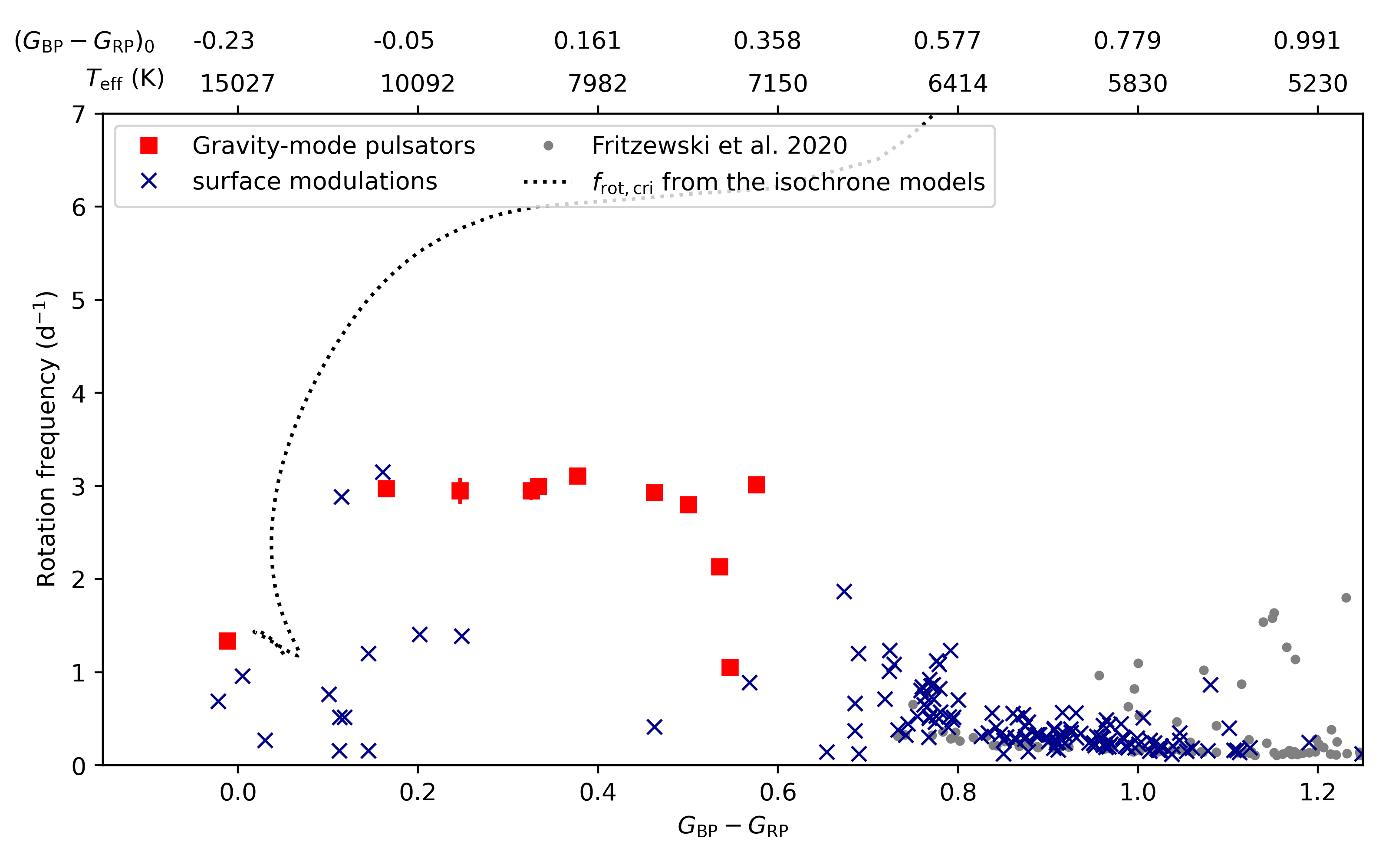
Figure 12: Observed rotation rates for cluster members from surface modulations or g-mode pulsations as a function of colour index. The y-axis is the rotation frequency in $\mathrm{d}^{-1}$. The bottom x-axis shows the observed Gaia colour index, while the top x-axis shows both the effective temperature and the intrinsic Gaia colour index from the best-fitting isochrone. The red squares show cluster members with near-core rotation rates measured from their identified g modes, while the dark blue crosses are stars with surface rotation measurements from modulations in their light curves. Rotation uncertainties are typically smaller than the marker sizes. The grey dots are the surface rotation rates for the late-type stars used for gyrochronology in the cluster reported by Fritzewski et al. (2020). The black dotted line represents the Keplerian critical rotation rate $f_{\mathrm{rot,cri}}$ from the best-fitting isochrone model.

In this section, we want to give the relation between stellar rotation rates and their colour index $G_{\mathrm{BP}}-G_{\mathrm{RP}}$. The peaks of the fundamental frequencies in the cluster stars with rotational modulation directly give the surface rotation rates, while the g-mode period spacings deliver the near-core rotation rates. We can compare them together because the radial differential rotations in main-sequence stars are not strong (e.g. Li et al., 2020b).

We want to measure the surface rotation of stars for two reasons: firstly, to slightly extend the samples of rotation beyond the red edge of the instability strip, and secondly, to compare with the near-core rotation measured through asteroseismology in order to determine the mild radial differential rotation of stars. We use the stars with these measurements to investigate how the rotation rates change as a function of colour index, which represents the effective temperature.

To properly determine the frequency and uncertainty of a surface modulation signal, we adopt a strategy akin to that used for solar-like oscillators. The surface activity, excited and damped over time, performs similar to the stochastically excited oscillations observed in solar-like oscillators. Consequently, a critically sampled power spectrum of a surface modulation signal is expected to exhibit a Lorentzian profile, with the data following a $\chi^{2}$ distribution with two degrees of freedom (Anderson et al., 1990). The likelihood function, which quantifies the probability of observed data $D$ given a parameter $\theta$ (see Anderson et al., 1990), is given by the equation:

$$\ln p(D|\theta)=-\sum\left(\ln M_{i}(\theta)+\frac{D_{i}}{M_{i}(\theta)}\right),$$ (8)

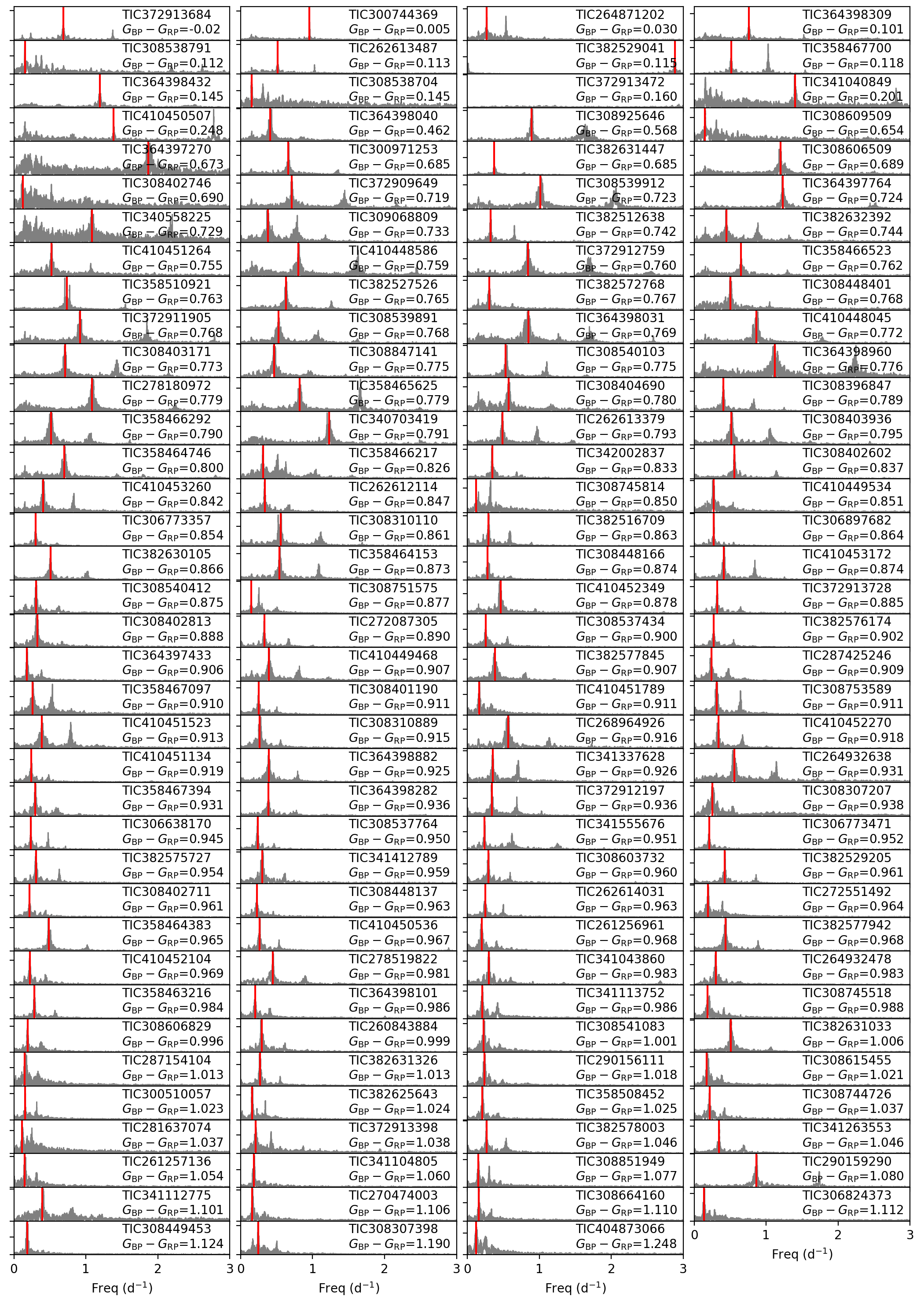
Figure 17: Surface modulation signals in the stars of NGC 2516, sorted by Gaia colour index. Stars with smaller colour indices are displayed at the top. Frequency (in $\mathrm{d^{-1}}$) is plotted along the x-axis. The y-axis, representing amplitude, is omitted for brevity. Each panel displays the amplitude spectrum in grey, with the rotation frequency indicated by a vertical red line. The TIC number and corresponding Gaia colour index are noted in each panel.

where $D_{i}$ represents the $i^{\mathrm{th}}$ data point, and $M_{i}(\theta)$ denotes the Lorentzian profile. The Lorentzian profile’s parameters, $\theta$, include the central frequency (which is the surface rotation frequency we want to measure), amplitude, Full Width Half Maximum (FWHM), and background noise. We used the emcee package (Foreman-Mackey et al., 2013) to optimise the likelihood function in Eq. 8, which is an implementation of the affine-invariant ensemble sampler of Goodman & Weare (2010). In the MCMC algorithm, we used 30 parallel chains and 5000 steps, and discarded the first 1000 steps for the final posterior distributions. We visually inspected all the posterior distributions to ensure all the chains converged. The determined surface rotation frequencies and their uncertainties are listed in Table 4, and all the surface modulation signals are illustrated in Fig. 17. The uncertainties of these frequencies are on the order of $10^{-3}$ to $10^{-4}\,\mathrm{d^{-1}}$, roughly akin to the frequency resolution of the 4-year light curve ($\sim 0.0007\,\mathrm{d^{-1}}$). In contrast, the uncertainties of stable oscillation signals (where amplitude, frequency, and phase remain constant) are significantly smaller. These are influenced by the signal-to-noise ratio and are typically less than one-tenth of the frequency resolution (Montgomery & O’Donoghue, 1999). Figure 16 compares the surface modulation periods in this work and those from Fritzewski et al. (2020), Bouma et al. (2021), and Healy & McCullough (2020), and a general consistency is seen.

In Fig. 12, we present the measured rotation rates as a function of colour index. For the cool stars (with $G_{\mathrm{BP}}-G_{\mathrm{RP}}>0.6$ mag), their rotation rates increase with increasing temperature. The rotation rate reaches approximately $1\,\mathrm{d^{-1}}$ at $G_{\mathrm{BP}}-G_{\mathrm{RP}}\approx 0.7$ mag, indicating the diminishing effect of magnetic braking. The stars with g-mode pulsations occur in the $G_{\mathrm{BP}}-G_{\mathrm{RP}}$ range of 0.2 mag to 0.6 mag, where rotational modulation is less common. Given the weak radial differential rotation found in hundreds of intermediate-mass stars (Li et al., 2020b), it is reasonable to compare the rotation rates for all cluster stars having measurements for either the near-core region or the surface. The near-core rotation rates measured by g modes are approximately $3\,\mathrm{d^{-1}}$, significantly faster than those derived for the cooler stars with magnetic braking. For stars with $G_{\mathrm{BP}}-G_{\mathrm{RP}}<0.2$ mag, both the rotation rates measured by surface modulation and g-mode pulsations decrease dramatically, displaying a large scatter of approximately $1.5\,\mathrm{d^{-1}}$, which might be suppressed by the critical rotation rates, as discussed below.

In addition, we have calculated the critical rotation rates, which we define as the rate at which the centrifugal and gravitational accelerations at the equator on an isobar are equal (see the definition in Paxton et al., 2019). To simplify the calculation, we ignored the ellipsoidal distortion, that is

$$\Omega_{\mathrm{crit}}=2\pi f_{\mathrm{rot,crit}}=\sqrt{\frac{\mathrm{G}M}{R^{3}}},$$ (9)

where $\mathrm{G}$ is the gravitational constant, $M$ is the stellar mass, and $R$ is the radius. We used the theoretical radii and masses obtained from the best-fitting isochrone stellar model (dotted line in Fig. 12).

The critical rotation rates obtained by best-fitting isochrone reveal three distinct regimes in Fig. 12. First, a decreasing trend is observed when $G_{\mathrm{BP}}-G_{\mathrm{RP}}$ exceeds 0.6 mag, declining to approximately $6\,\mathrm{d^{-1}}$, which represents the transition region from late-type to early-type stars; second, a relatively constant value is maintained between 5 and $6\,\mathrm{d^{-1}}$ within the $G_{\mathrm{BP}}-G_{\mathrm{RP}}$ range of 0.2 mag to 0.6 mag, where $\gamma$ Dor and $\delta$ Sct stars occur; third, a rapid decline is observed for $G_{\mathrm{BP}}-G_{\mathrm{RP}}<0.2$ mag, with the critical rotation rate dropping to approximately $2\,\mathrm{d^{-1}}$, which coincides with the main-sequence turn-off of the cluster, where a few surface modulation stars and one SPB star appear.

Within the region of $G_{\mathrm{BP}}-G_{\mathrm{RP}}$ between 0.2 mag and 0.6 mag, the rotation rates measured for the g-mode pulsators correspond approximately to 50% of the critical rotation rates. As pointed out by Mombarg et al. (2021) and (Henneco et al., 2021), the TAR is still valid for $\Omega/\Omega_{\mathrm{crit,Roche}}$ up to 0.8, where $\Omega_{\mathrm{crit,Roche}}=\sqrt{8/27}\Omega_{\mathrm{crit}}$. Mombarg (2023) found that the initial rotation frequencies of six slowly rotating field $\gamma\,$Dor stars near the terminal age main sequence must have originated from stars rotating below 10% of the initial critical frequency at the zero-age main sequence. Our values of $\Omega/\Omega_{\mathrm{crit}}\approx 0.5$ show that the $\gamma\,$Dor stars in NGC 2516 are born with five times higher rotation rate. At NGC 2516’s turn-off, the rotation rates closely approach the critical rate, which is consistent with the findings by Aerts (2021) that all rotation rates, from zero to critical, are observed between stellar birth and the end of the main sequence. Our findings are also consistent with some spectropolarimetric observations of Be stars (e.g. Regulus, Achernar, and $\alpha$ Arae, see McAlister et al., 2005; Domiciano de Souza et al., 2003; Meilland et al., 2007).

The theoretical critical rotation rates derived from isochrone models are approximately 1 $\mathrm{d^{-1}}$ higher than the observed critical rotation rates, revealing a systematic deviation. This deviation is easily understood in terms of a variety of choices for the input physics of the models, notably the occurrence of major differences in internal mixing (Pedersen et al., 2021). Moreover, part of this systematic shift may arise from the neglected gravity darkening or centrifugal distortion of the fast rotation of the cluster stars, making it challenging to precisely define their $T_{\mathrm{eff}}$, $\log g$, and radius. In Sect. 3, we determined that the best-fitting isochrones have $\Omega/\Omega_{\mathrm{crit}}\leq 0.4$, a finding that is incompatible with the value derived from g-mode pulsators. This discrepancy is likely due to the inaccurate determination of $\Omega_{\mathrm{crit}}$.

4.7 No circumstellar disk around the fast-rotating B stars

Fast-rotating stars may experience disk formation events due to outbursts that eject surface material from their equator into a decretion disk. This phenomenon, commonly known as the Be phenomenon, has been observed for the Be star HD 49330 (Huat et al., 2009). Such decretion events can e triggered by the beating of g-mode pulsations (Kurtz et al., 2015). Notably, Neiner et al. (2020) also showed that the beating of the stochastically-excited gravito-inertial waves in HD 49330 is efficient for transporting the angular momentum from the core to the surface, causing the Be phenomenon. If similar Be phenomena are observed in the rapid rotators within our sample, the asteroseismology data might offer further insights into the mechanisms triggering these occurrences.

Outburst akin to the one detected in the optical CoRoT light curve of HD 49330 can also be detected at mid-infrared wavelengths, such as the Wide-field Infrared Survey Explorer (WISE; Wright et al. 2010) photometry bands $W1$ and $W2$. This wavelength range notably contains the primary emissions from the decretion disk. Granada et al. (2018) found that around half of the B-type stars in four young clusters have $W1-W2$ colours redder than $0.05$, while the intrinsic colours of early-type stars are around $-0.05$. Jian et al. (2023) confirmed this conclusion, identifying 916 early-type stars that have shown outbursts associated with the Be phenomenon over the past 13 years. Given the presence of fast rotators in NGC 2516, it’s plausible that some of them might experience Be phenomena, potentially be captured in their WISE photometry.

Following the method introduced by Jian et al. (2023), we extracted the WISE epoch photometry for all our sample stars. Figure 13 presents the colour-magnitude diagram with the median and extreme values derived from the WISE photometry for our sample of cluster members. Stars exhibiting the Be phenomena typically display a ”redder and brighter” variation in their photometry. Their median $(W1-W2)$ will then range from $0$ to $0.3\text{\,}\mathrm{m}\mathrm{a}\mathrm{g}$, and the vertical bar in Figure 13 can extend up to $1.5\text{\,}\mathrm{m}\mathrm{a}\mathrm{g}$ (see Figure 9 in Jian et al. 2023 for comparison). Our analysis revealed that none of the stars within NGC 2516 demonstrated such behaviour. It’s important to note that the larger $(W1-W2)$ observed at $W1>12\,$mag corresponds to stars with lower effective temperatures, where their redder colours stem from the presence of molecular lines in the $W1$ band rather than from the Be phenomenon.

The reason for the absence of the Be phenomenon in NGC 2516 is still uncertain, but there are potential reasons worth considering. One possibility might be the relatively old age of NGC 2516. There are 35 Be stars reported in Jian et al. (2023) that are associated with open clusters, and most of these clusters’ ages fall below 45 million years, which is less than half the age of NGC 2516. Another possible reason might be the rotation rate. The rotation rates we found for the A-type stars of NGC 2516 are roughly at about 50% of the critical rate. However, as shown in Fig. 12, the B-type stars (with $G_{\mathrm{BP}}-G_{\mathrm{RP}}<0.2\,\mathrm{mag}$) exhibit much larger $\Omega/\Omega_{\mathrm{crit}}$ due to the decrease in critical rotation rates at the MSTO. The critical rotation rate at the MSTO is hard to determine, because of the rapid change in stellar physics. Therefore, it is still unclear if the rotation rates of our B-type stars are sufficient to induce the formation of decretion disks. It’s noteworthy that some field SPB stars observed by Kepler display minor outbursts in their light curve despite the absence of disks (Van Beeck et al., 2021), indicating that additional factors beyond rotation may contribute to the occurrence or absence of the Be phenomenon (see earlier comment on Kurtz et al., 2015).

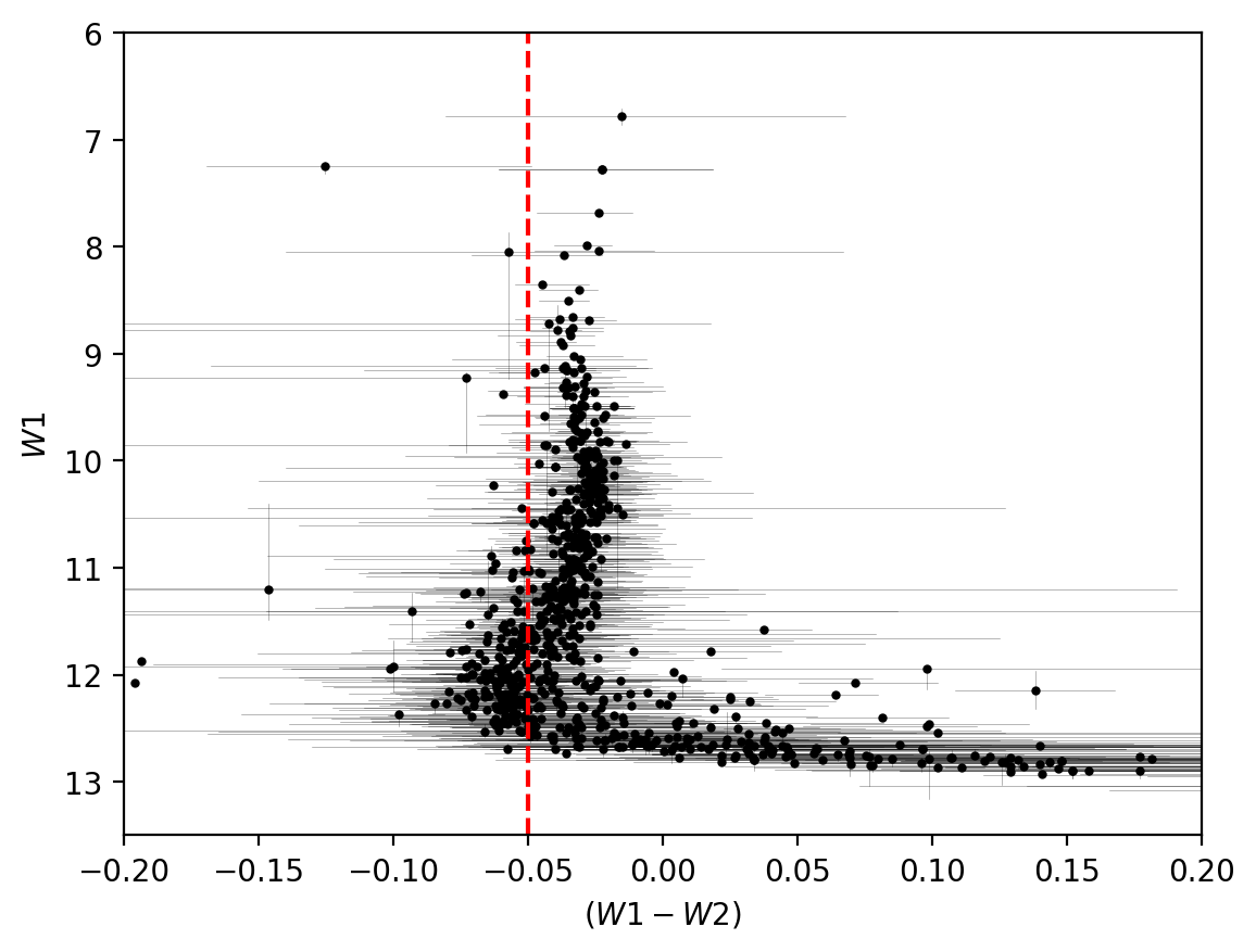
Figure 13: WISE colour-magnitude diagram of the sample stars, with the median value of $(W1-W2)$ and $W1$ plotted as black dots, and their extreme values plotted as horizontal and vertical errorbars. The red dashed-vertical line indicates the intrinsic colour ($-0.05$) of the stars with $T_{\mathrm{eff}}>6000$ K.

5 Spectroscopic observations

To accomplish the goal of calibrating stellar models through detailed asteroseismic modelling of the g-mode pulsators in NGC 2516 with methods as in Aerts et al. (2018), relying solely on photometric and Gaia observations are sub-optimal. High-resolution spectroscopic observations, delivering better constraints on $T_{\rm eff}$, $\log g$, and metallicity offer a powerful addition as observables. Accurate measurements of parameters such as $T_{\mathrm{eff}}$, metallicity, and $\log g$ not only narrow down the range of possible models but also help resolve degeneracies in the high-dimensional parameter space. Additionally, measurements of surface element abundances play a crucial role in constraining the internal mixing processes within radiative envelopes, as demonstrated in previous studies (Pedersen et al., 2018; Mombarg et al., 2020, 2022; Pedersen et al., 2021; Michielsen et al., 2021).

For these reasons, we aimed to collect high-resolution spectra of the most interesting cluster members. Given their high potential for cluster modelling, we focused on the g-mode pulsators exhibiting clear period spacing patterns in this cluster and reported the data assembled so far. We conducted spectroscopic follow-up observations using the Fibre-fed Extended Range Optical Spectrograph (FEROS) (Kaufer et al., 1999), which is mounted on the ESO/MPG 2.2-m telescope at La Silla, Chile. FEROS is a high-resolution spectrograph with an approximate resolution ($R$) of 48,000 and a wavelength coverage from 360 to 920 nm. The data reduction was performed using the publicly available pipeline Collection of Elemental Routines for Échelle Spectra (CERES) (Brahm et al., 2017). All the spectra and the best-fitting results are shown in Sect. B.

We derived the global parameters, including radial velocity, $T_{\mathrm{eff}}$, $\log g$, projected equatorial rotation velocity ($v\sin i$), microturbulent velocity in the atmosphere($\xi$), and metallicity ([M/H]), using the spectrum analysis algorithm zeta-Payne (Straumit et al., 2022). This algorithm is fully automated and machine-learning-based, specifically optimised for intermediate- to high-mass stars with spectral types O, B, A, and F and optimally suited to exploit FEROS spectroscopy of g-mode pulsators (Gebruers et al., 2022). The observational details and parameter results are summarised in Table 3. These observations were conducted between 12th and 16th of March, 2023, with varying exposure times of 600, 900, and 1800 s, depending on the brightness of the target star. We aimed for a high signal-to-noise ratio (S/N) of 200 to ensure accurate abundance determinations. In cases where achieving S/N=200 with a single exposure time was not feasible for faint stars, we combined multiple shorter exposures with S/N=150 to reach the desired S/N=200. However, it is worth noting that we still did not achieve a high S/N for some stars, such that follow-up measurements are still needed to get precise values of the stellar parameters.

As demonstrated by Gebruers et al. (2022), internal uncertainties occur in the spectrum analysis, in addition to statistical uncertainties, even when the S/N is high. Therefore, we calculated the uncertainties in surface parameters and radial velocity by quadratic summation of the observed and internal uncertainties. Figure 14 contains a comparison between the effective temperatures obtained from the FEROS spectra and those derived using the Gaia General Stellar Parametrizer from Photometry (GSP-Phot). Our analysis reveals that the temperatures derived from the spectra exhibit a smoother relation with the Gaia colour index, whereas the GSP-Phot temperatures display considerable scatter. In some cases, this scatter is as high as approximately $2000\,\mathrm{K}$. Furthermore, we determined the metallicities of these stars and found them to align with solar metallicity within the uncertainties. The radial velocities (RV) of the stars also exhibit consistency, averaging around $\sim 25\,\,\pm\sim 7\,\mathrm{km/s}$, consistent with González & Lapasset (2000). Notably, multiple observations of the same target stars do not reveal significant RV variations, excluding short-period binarity among the monitored stars.

Table 3: Results of the spectroscopic observations of the g-mode pulsators in NGC 2516. Some stars were observed more than once.

TIC	DATE-OBS	EXP	$m_{\mathrm{g}}$	BP-RP	S/N	RV (km/s)	$T_{\mathrm{eff}}$ (K)	$\log g$ (dex)	$v\sin i$ (km/s)	$\xi$ (km/s)	[M/H] (dex)
281582674	2023-03-12	1800	10.36	0.38	101	$26\pm 20$	$8100\pm 300$	$3.97\pm 0.21$	$274\pm 24$	$3.1\pm 2.0$	$0.02\pm 0.20$
281582674	2023-03-16	1800	10.36	0.38	121	$25\pm 12$	$8100\pm 300$	$3.95\pm 0.20$	$274\pm 23$	$3.2\pm 1.9$	$-0.01\pm 0.20$
308307454	2023-03-13	1800	11.20	0.55	56	$24\pm 4$	$7220\pm 220$	$3.8\pm 0.4$	$56\pm 12$	$2.8\pm 1.4$	$-0.27\pm 0.21$
308307454	2023-03-14	1800	11.20	0.55	77	$23\pm 3$	$7250\pm 220$	$3.7\pm 0.3$	$56\pm 12$	$3.0\pm 1.4$	$-0.32\pm 0.21$
308307454	2023-03-16	1800	11.20	0.55	67	$25\pm 3$	$7250\pm 220$	$3.7\pm 0.4$	$55\pm 12$	$2.9\pm 1.4$	$-0.31\pm 0.21$
358466708	2023-03-12	600	8.05	-0.01	191	$27\pm 5$	$12070\pm 170$	$3.83\pm 0.06$	$181\pm 16$	$0.6\pm 2.0$	$0.08\pm 0.16$
358466729	2023-03-13	1800	11.15	0.54	81	$24\pm 6$	$7140\pm 220$	$4.1\pm 0.4$	$129\pm 14$	$2.3\pm 1.4$	$-0.11\pm 0.21$
358466729	2023-03-15	1800	11.15	0.54	91	$22\pm 4$	$7160\pm 220$	$4.1\pm 0.3$	$130\pm 13$	$2.4\pm 1.4$	$-0.11\pm 0.21$
364398040	2023-03-13	1800	10.50	0.46	92	$22\pm 8$	$7590\pm 220$	$3.9\pm 0.4$	$271\pm 18$	$3.9\pm 1.4$	$-0.12\pm 0.20$
364398040	2023-03-15	1800	10.50	0.46	140	$18\pm 4$	$7610\pm 220$	$3.9\pm 0.3$	$274\pm 15$	$4.0\pm 1.3$	$-0.09\pm 0.20$
372912679	2023-03-14	1800	10.37	0.33	130	$24\pm 7$	$8500\pm 300$	$4.19\pm 0.19$	$134\pm 21$	$3.2\pm 2.0$	$-0.11\pm 0.19$
372912679	2023-03-15	1800	10.37	0.33	156	$24\pm 7$	$8500\pm 300$	$4.21\pm 0.19$	$134\pm 20$	$3.3\pm 2.0$	$-0.13\pm 0.19$
372913043	2023-03-12	900	8.74	0.17	144	$22\pm 4$	$11510\pm 240$	$4.12\pm 0.11$	$96\pm 19$	$0.9\pm 2.3$	$0.09\pm 0.22$
410451583	2023-03-14	1800	9.58	0.33	218	$26\pm 6$	$8300\pm 300$	$3.91\pm 0.18$	$304\pm 20$	$3.2\pm 1.9$	$-0.21\pm 0.18$
410452218	2023-03-14	1800	10.86	0.50	83	$23\pm 12$	$7900\pm 300$	$3.92\pm 0.23$	$272\pm 27$	$2.4\pm 2.0$	$0.12\pm 0.22$
410452218	2023-03-16	1800	10.86	0.50	86	$24\pm 13$	$7900\pm 220$	$3.9\pm 0.3$	$268\pm 18$	$2.3\pm 1.4$	$0.16\pm 0.21$

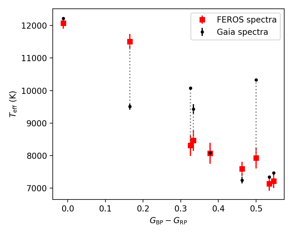
Figure 14: Effective temperature of the g-mode stars as a function of their Gaia colour index. We show the effective temperatures obtained by the FEROS spectra and Gaia GSP-Phot connected by vertical dotted line.

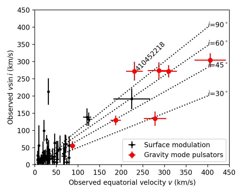
Figure 15: Comparison between the observed equatorial velocity and the observed $v\sin i$ by Gaia. For the surface modulation stars (black dot symbols), the $v\sin i$ comes from the Gaia’s vbroad parameter, and the $v$ is calculated using the rotation frequency and stellar radius. For the g-mode pulsators (red circle symbols), the $v\sin i$ are measured by the FEROS spectra, and their $v$ is calculated by the near-core rotation rate and stellar radius. The dotted lines mark the locations with various inclinations.

Figure 15 illustrates the comparison between various estimates of the projected equatorial rotation velocity ($v\sin i$) and the true equatorial velocity for several of the cluster members. This provides a direct estimate of the inclination of the rotation axis of the stars in the line of sight. Various remarks are in order. For stars exhibiting surface modulations, we have a direct determination of the surface rotation period. We computed their equatorial velocities by multiplying with the radii as determined in Section 4.5. Additionally, we obtained their projected equatorial velocities using the vbroad parameter provided by the Gaia Radial Velocity Spectrometer (RVS) (Frémat et al., 2023b). For stars displaying period spacing patterns with identified g-mode pulsations, we have the near-core rotation rates and the $v\sin i$ values were measured from FEROS spectra. For these stars, we recalculated their radii using the more accurate effective temperatures derived from the FEROS spectra. We then determined their equatorial velocities by multiplying their radii with the near-core rotation rates, assuming these stars have rigid rotation. Figure 15 reveals that most stars with surface modulations have low $v\sin i$ values not significantly different from zero, indicative of slow rotation. When the equatorial velocity surpasses approximately $100\,\mathrm{km/s}$, the stars have $v\sin i$ values significantly above zero. We find that these stars cover a range of inclinations, spanning from approximately $30^{\circ}$ to $90^{\circ}$. Although it concerns relatively a few cluster members, most of the stars with inclination estimates have values $i\gtrsim 45^{\circ}$, resembling a distribution akin to random orientations. It is worth noting that TIC 410452218 is the only star for which the projected equatorial velocity ($v\sin i$) is larger than the equatorial velocity. This discrepancy might be due to poor consideration of rotational distortion or gravity darkening.

We stress that the determination of the inclination angles comes with a significant degree of uncertainty. First, it is important to note that in the case of rapidly rotating stars, there are variations in both radius and temperature between the pole and equator. Therefore, the radius determined through the Stefan-Boltzmann law should be considered as an averaged value that is also influenced by the effective temperature and inclination. Secondly, differential rotation may occur while we have assumed rigid rotation for the g-mode pulsators. Observations have indicated that the difference between the near-core and surface rotation rates typically does not exceed 10% for $\gamma\,$Dor stars from the Kepler field (Li et al., 2020b), but these stars are much older than those in NGC 2516. However, recent two-dimensional models suggest a more complex internal rotation profile and show that the core might rotate approximately 50% faster than the envelope (Bouchaud et al., 2020; Mombarg et al., 2023). This level of differentiality in the rotation adds to the complexity and uncertainty in determining the inclination angles in these cases.

6 Conclusions

In this study, we conduct the first asteroseismic study of the young open cluster NGC 2516. Our findings reveal a variety of different types of variable stars in this cluster. These stars, along with the cluster itself, can help us calibrate the physics processes inside stars to unprecedented precision and answer long-standing questions about star clusters.

Firstly, we applied the rotating MIST isochrones to fit the color-magnitude diagram (CMD) of the cluster. We find that isochrones with $\Omega/\Omega_{\mathrm{crit}}\leq 0.4$ closely matched the observational data and yielded consistent results for age and extinction. However, those with $\Omega/\Omega_{\mathrm{crit}}\geq 0.5$ did not provide a good fit to the data. By combining the fitting results obtained from isochrones with $\Omega/\Omega_{\mathrm{crit}}\leq 0.4$, we report an age of $102\pm 15\,\mathrm{Myr}$ and an extinction value at 550 nm of $A_{0}=0.53\pm 0.04\,\mathrm{mag}$. Our newly determined age shows that NGC 2516 is younger than the Pleiades, while we provide a slightly larger extinction and reddening than the previous study.

We used the TESS data in cycle 1 and cycle 3 to conduct photometry and obtained the light curves of the member stars. The almost continuous TESS light curves provided excellent data for asteroseismology. We find 24 g-mode pulsators, 35 $\delta$ Sct pulsators, 147 stars with surface modulations, 5 eclipsing binaries, and three post-main-sequence stars.

Among the g-mode pulsators, there are 11 with clear period spacing patterns, which allow us to determine their near-core rotation rates and asymptotic spacings. We identified most of these stars as $\gamma$ Dor stars based on their asymptotic spacings (around $\sim 5000\,\mathrm{s}$) and effective temperatures (between 7000 K and 10000 K). Their asymptotic spacings are larger than those $\gamma$ Dor stars in the Kepler field because they are young. Additionally, there are two stars with even higher effective temperatures ($>10000\,\mathrm{K}$). Considering the position of these stars at the top of the main sequence, we classified them as SPB stars. Our findings reveal that the g-mode stars in NGC 2516 exhibit rapid near-core rotation rates, some reaching values up to $3\,\mathrm{d^{-1}}$. This is significantly faster than the average value for those observed for single pulsators in both the Kepler and TESS fields. The combination of a large asymptotic period spacing and high near-core rotation rates aligns with the nature that these stars are very young.

For the $\delta$ Sct stars, we observe that their amplitude spectra are well ordered when sorted by colour. In cooler stars, we find a series of frequencies at approximately $21.07\,\mathrm{d^{-1}}$, while the hotter p-mode pulsators display another series of frequency peaks around $33\,\mathrm{d^{-1}}$. These frequencies are identified as the fundamental frequency and second overtone, respectively. Notably, the mean pulsation frequency increases as the temperature rises, indicating a frequency – temperature relation in $\delta$ Sct stars. We cannot identify reliable frequency separations among these $\delta$ Sct stars, except for one cluster member.

For the three post-main-sequence stars, we observe a low-frequency power excess in their power density spectra in agreement with theoretical predictions for granulation resulting from magnetic activity. Based on the closest model from the best-fitting isochrone, these evolved stars have masses larger than $5\,\mathrm{M_{\odot}}$, which is greater than the most massive star from the Kepler sample (Yu et al., 2018).

The surface modulation signals observed in 147 stars offer direct measurements of surface rotation rates. Combined with near-core rotation rates determined from g-mode pulsations, we unveil a rotation – temperature relationship among the main-sequence stars in NGC 2516. Our findings show that as temperature increases, the typical rotation rate follows a rising trend until it reaches a plateau (whose red edge is at $G_{\mathrm{BP}}-G_{\mathrm{RP}}=0.6\,\mathrm{mag}$ or $T_{\mathrm{eff}}=7150\,\mathrm{K}$), where it stabilises at approximately 50% of the critical rotation rates. Furthermore, we calculate the critical rotation rates using both the best-fitting stellar models and observations. We observe a rapid drop in the critical rotation rate at the main-sequence turn-off, in agreement with the observed stellar rotation rates. It is noteworthy that the rotation rate in B-type stars may approach nearly $\sim 90\%$ of the critical rotation rate. However, we did not find any evidence of circumstellar disks in these cluster stars.

Finally, we carried out high-resolution spectroscopic observations for the g-mode pulsators displaying period spacing patterns. Our spectra, with high resolution and high S/N, enabled precise measurements of the global stellar parameters and radial velocity. Our analysis confirms that the cluster has solar metallicity and exhibits a radial velocity of approximately $\sim 25\,\mathrm{km/s}$. These accurate spectroscopic observations will provide invaluable information for our planned detailed ensemble asteroseismic modelling of the g-mode pulsators under the constraint of equal initial chemical composition at birth, reducing computational complexity and resolving parameter degeneracies.

NGC 2516 revealed itself as an optimal cluster for combined detailed asteroseismic modelling of its g-mode pulsators. So far such type of asteroseismic cluster modelling based on g-mode pulsators has not yet been done. The only young open cluster that was scrutinised by g-mode asteroseismology so far is UBC1, which has only one g-mode pulsator with identified modes (Fritzewski et al., 2023). Since the addition of one g-mode pulsator already implied a drastic reduction in the uncertainty of the cluster age, our future modelling of the eleven g-mode pulsators and the $\delta\,$Sct overtone pulsators in NGC 2516 promises to be extremely rewarding to increase our knowledge of the interior physics of intermediate-mass stars and young open clusters.

Appendix A Surface modulations

Figure 16 compares the surface modulation periods by this work and by the previous studies. We collected the results by Fritzewski et al. (2020), Bouma et al. (2021), and Healy & McCullough (2020). Our results show high consistency. Table 4 lists the periods of all the surface modulation stars. Figure 17 depicts all the surface modulation amplitude spectra.

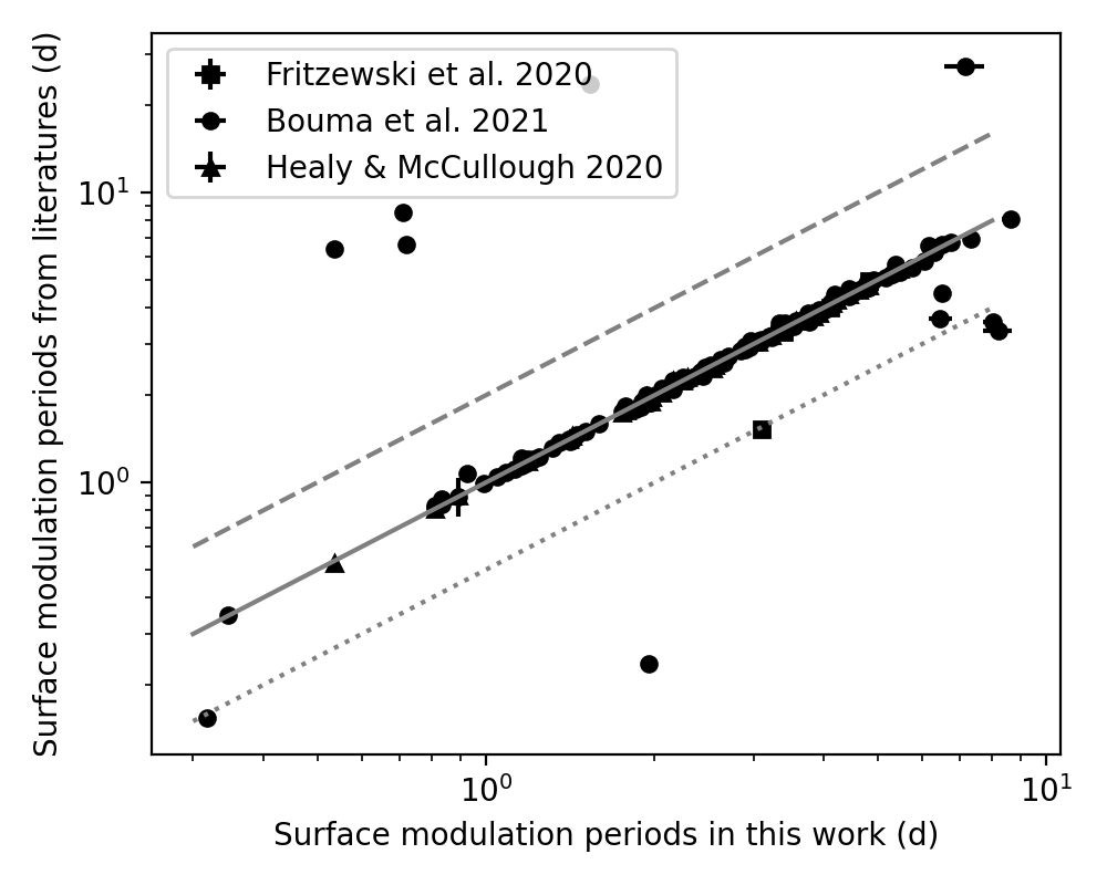
Figure 16: A comparison of the surface modulation periods in this work and from the previous literatures. We collected the results by Fritzewski et al. (2020), Bouma et al. (2021), and Healy & McCullough (2020). The grey solid, dashed, and dashed lines show the 1:1, 2:1, and 1:2 relations.

Table 4: Surface modulation periods for the cluster member stars in this study.

TIC	CI	Freq ($\mathrm{d^{-1}}$)	$P$ (d)	TIC	CI	Freq ($\mathrm{d^{-1}}$)	$P$ (d)	TIC	CI	Freq ($\mathrm{d^{-1}}$)	$P$ (d)	TIC	CI	Freq ($\mathrm{d^{-1}}$)	$P$ (d)
372913684	-0.022	0.6878(13)	1.4538(28)	300744369	0.005	0.9567(5)	1.0453(6)	264871202	0.030	0.2668(26)	3.75(4)	364398309	0.101	0.7612(17)	1.3137(29)
308538791	0.113	0.155(7)	6.5(3)	262613487	0.113	0.5131(6)	1.9488(24)	382529041	0.115	2.8807(12)	0.34714(14)	358467700	0.118	0.5154(15)	1.940(6)
364398432	0.145	1.198(3)	0.8350(22)	308538704	0.145	0.1535(29)	6.52(12)	372913472	0.161	3.1470(13)	0.31777(13)	341040849	0.202	1.4039(23)	0.7123(12)
410450507	0.249	1.3869(22)	0.7211(11)	364398040	0.463	0.410(4)	2.440(23)	308925646	0.569	0.888(5)	1.126(6)	308609509	0.654	0.140(11)	7.2(6)
364397270	0.674	1.869(7)	0.5352(21)	300971253	0.686	0.6631(13)	1.508(3)	382631447	0.686	0.3693(27)	2.708(20)	308606509	0.690	1.199(3)	0.8343(22)
308402746	0.690	0.125(5)	8.0(3)	372909649	0.719	0.7079(21)	1.413(4)	308539912	0.724	1.010(5)	0.990(5)	364397764	0.724	1.2315(22)	0.8120(15)
340558225	0.729	1.083(7)	0.923(6)	309068809	0.733	0.377(6)	2.65(4)	382512638	0.742	0.3231(12)	3.095(11)	382632392	0.745	0.445(4)	2.245(18)
410451264	0.755	0.522(4)	1.915(13)	410448586	0.759	0.803(3)	1.246(5)	372912759	0.760	0.8429(22)	1.186(3)	358466523	0.762	0.6512(18)	1.536(4)
358510921	0.763	0.7395(27)	1.352(5)	382527526	0.766	0.6284(18)	1.591(5)	382572768	0.768	0.3015(16)	3.317(18)	308448401	0.768	0.5050(26)	1.98(10)
372911905	0.769	0.920(3)	1.087(4)	308539891	0.769	0.526(6)	1.903(23)	364398031	0.770	0.849(4)	1.178(5)	410448045	0.772	0.8645(26)	1.157(3)
308403171	0.773	0.7111(24)	1.406(5)	308847141	0.775	0.465(4)	2.152(17)	308540103	0.776	0.528(3)	1.892(11)	364398960	0.777	1.120(6)	0.893(5)
278180972	0.779	1.083(3)	0.9231(29)	358465625	0.780	0.822(4)	1.216(5)	308404690	0.781	0.571(3)	1.752(9)	308396847	0.790	0.4061(15)	2.463(9)
358466292	0.790	0.518(4)	1.931(15)	340703419	0.792	1.231(3)	0.8127(20)	262613379	0.794	0.4849(16)	2.062(7)	308403936	0.795	0.514(4)	1.947(16)
358464746	0.801	0.7024(23)	1.424(5)	358466217	0.826	0.311(4)	3.21(4)	342002837	0.834	0.3457(25)	2.893(21)	308402602	0.838	0.5607(25)	1.783(8)
410453260	0.843	0.407(4)	2.459(21)	262612114	0.847	0.3341(25)	2.993(23)	308745814	0.851	0.122(7)	8.2(5)	410449534	0.851	0.2689(25)	3.72(3)
306773357	0.854	0.3024(9)	3.31(10)	308310110	0.861	0.5572(22)	1.795(7)	382516709	0.864	0.2937(15)	3.405(17)	306897682	0.864	0.2721(11)	3.675(14)
382630105	0.866	0.5118(20)	1.954(8)	358464153	0.873	0.5403(22)	1.851(8)	308448166	0.874	0.2800(17)	3.572(21)	410453172	0.875	0.4145(19)	2.413(11)
308540412	0.875	0.3088(25)	3.238(26)	308751575	0.878	0.1480(22)	6.8(10)	410452349	0.878	0.464(4)	2.156(16)	372913728	0.886	0.3221(20)	3.105(20)
308402813	0.888	0.326(3)	3.07(3)	272087305	0.891	0.3283(11)	3.05(10)	308537434	0.901	0.2544(17)	3.930(27)	382576174	0.902	0.2709(21)	3.691(29)
364397433	0.906	0.1823(19)	5.49(6)	410449468	0.907	0.3944(22)	2.536(14)	382577845	0.907	0.381(4)	2.627(29)	287425246	0.909	0.2390(24)	4.18(4)
358467097	0.910	0.260(4)	3.85(5)	308401190	0.911	0.2488(17)	4.019(27)	410451789	0.912	0.1652(18)	6.05(7)	308753589	0.912	0.3124(20)	3.201(20)
410451523	0.914	0.386(5)	2.59(4)	308310889	0.915	0.2655(22)	3.77(3)	268964926	0.916	0.564(4)	1.774(13)	410452270	0.918	0.3369(26)	2.968(23)
410451134	0.919	0.2409(16)	4.151(28)	364398882	0.926	0.3904(24)	2.562(15)	341337628	0.926	0.3505(21)	2.853(17)	264932638	0.931	0.560(4)	1.785(12)
358467394	0.932	0.294(5)	3.40(5)	364398282	0.936	0.3846(21)	2.600(14)	372912197	0.937	0.340(3)	2.945(28)	308307207	0.938	0.254(5)	3.94(8)
306638170	0.946	0.2379(13)	4.203(23)	308537764	0.951	0.2363(29)	4.23(5)	341555676	0.951	0.2385(23)	4.19(4)	306773471	0.952	0.2089(18)	4.79(4)
382575727	0.954	0.3088(16)	3.239(17)	341412789	0.959	0.300(3)	3.34(4)	308603732	0.960	0.2912(24)	3.434(28)	382529205	0.962	0.4236(29)	2.361(16)
308402711	0.962	0.2161(20)	4.63(4)	308448137	0.963	0.2249(21)	4.45(4)	262614031	0.964	0.2461(16)	4.063(26)	272551492	0.965	0.1935(18)	5.17(5)
358464383	0.965	0.485(3)	2.064(13)	410450536	0.968	0.2625(16)	3.809(24)	261256961	0.968	0.1972(29)	5.07(7)	382577942	0.969	0.437(3)	2.288(16)
410452104	0.970	0.2251(21)	4.44(4)	278519822	0.981	0.444(4)	2.252(22)	341043860	0.983	0.2969(28)	3.37(3)	264932478	0.983	0.299(4)	3.34(4)
358463216	0.984	0.2830(16)	3.534(20)	364398101	0.986	0.2031(18)	4.92(4)	341113752	0.987	0.206(4)	4.9(10)	308745518	0.989	0.1882(24)	5.31(7)
308606829	0.997	0.1895(18)	5.28(5)	260843884	0.999	0.292(3)	3.42(4)	308541083	1.001	0.2252(27)	4.44(5)	382631033	1.006	0.5080(21)	1.968(8)
287154104	1.013	0.150(8)	6.7(4)	382631326	1.013	0.2674(18)	3.740(25)	290156111	1.019	0.239(3)	4.18(6)	308615455	1.021	0.174(4)	5.75(14)
300510057	1.023	0.1588(14)	6.30(6)	382625643	1.025	0.1625(15)	6.15(6)	358508452	1.026	0.2079(27)	4.81(6)	308744726	1.038	0.2135(26)	4.68(6)
281637074	1.038	0.116(4)	8.6(3)	372913398	1.039	0.2071(29)	4.83(7)	382578003	1.046	0.2664(21)	3.75(3)	341263553	1.046	0.3443(17)	2.904(14)
261257136	1.054	0.152(4)	6.56(18)	341104805	1.060	0.1853(29)	5.40(8)	308851949	1.078	0.1538(19)	6.50(8)	290159290	1.081	0.864(3)	1.158(4)
341112775	1.102	0.397(5)	2.52(3)	270474003	1.107	0.1615(29)	6.19(11)	308664160	1.110	0.1601(19)	6.24(7)	306824373	1.113	0.1364(23)	7.33(12)
308449453	1.125	0.1856(20)	5.39(6)	308307398	1.190	0.243(5)	4.11(8)	404873066	1.249	0.124(3)	8.10(23)

Appendix B All the g-mode pulsators in NGC 2516

For each of the 11 g-mode pulsators, we show the amplitude spectrum with identified period spacing pattern, the best-fitting TAR results and the posterior distributions of $f_{\mathrm{rot}}$ and $\Pi_{0}$. We also show all the high-resolution spectra for these stars.

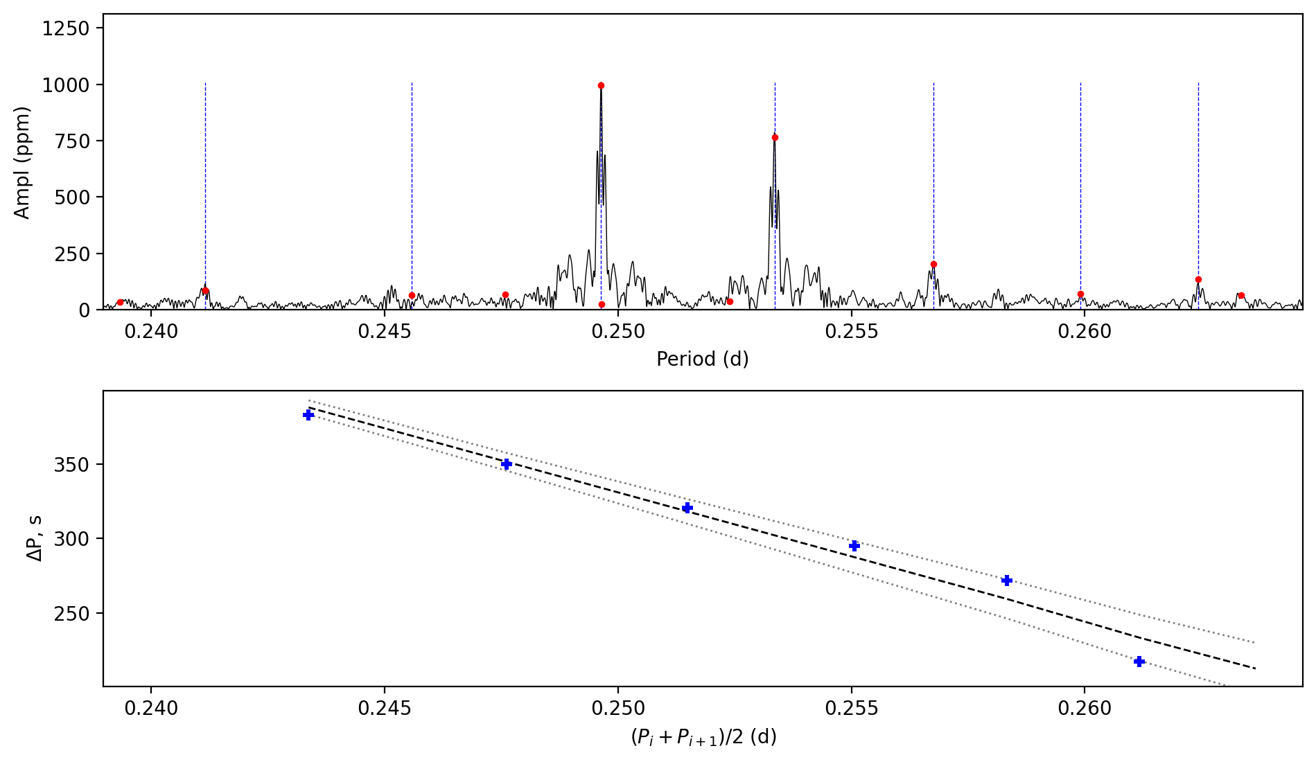
Figure 18: Period spacing pattern(s) of TIC 281582674. Top: amplitude spectrum as a function of period. Red dots are the peaks from the prewhitening process. Vertical lines mark the identified modes. Bottom: period spacing as a function of period. The black line is a linear fitting not the TAR fitting, and the grey lines exhibit the uncertainty region. The period is plotted as the mean value of the two consecutive peaks.

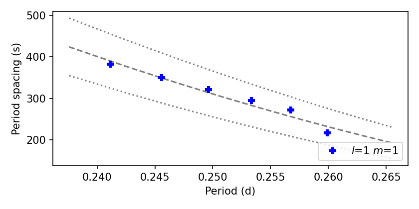
Figure 19: Period spacing pattern(s) from the TAR fitting of TIC 281582674. The dashed line marks the best-fitting model while the dotted lines exhibit the uncertainty region.

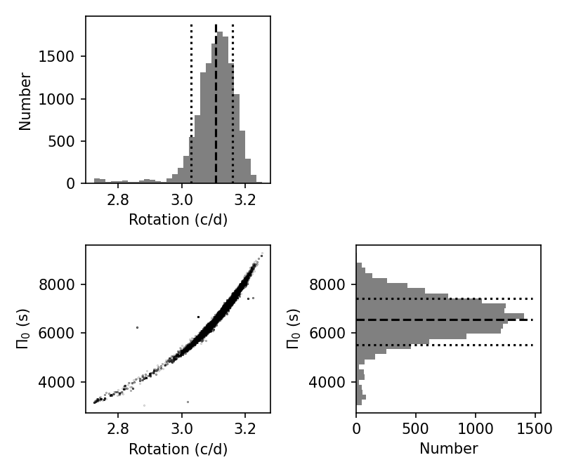
Figure 20: Posterior distributions of the TAR fitting of TIC 281582674.

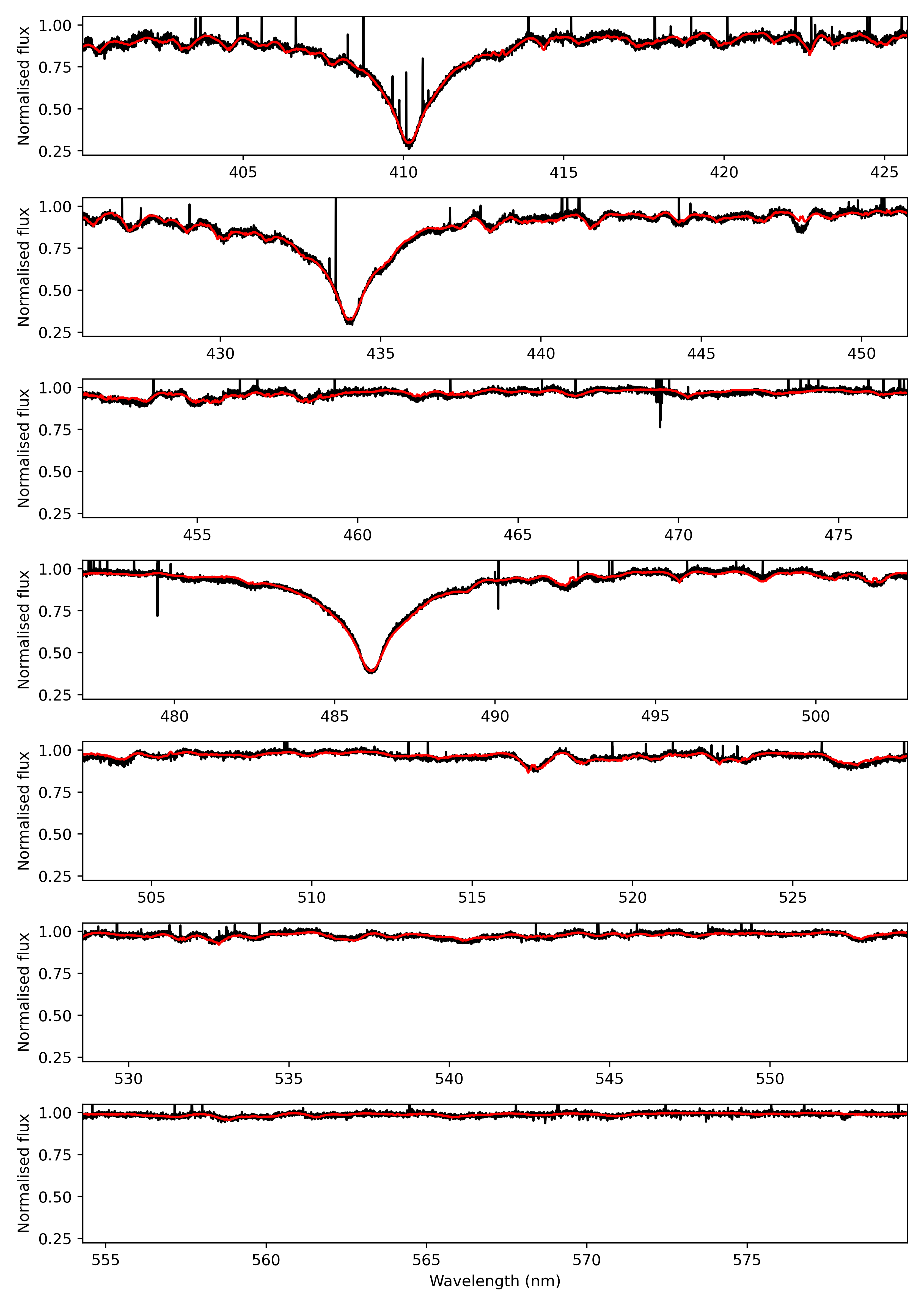
Figure 21: Spectrum of TIC 281582674 observed at 2023-03-12T23:47:34.131. The red line is the best-fitting theoretical spectrum.

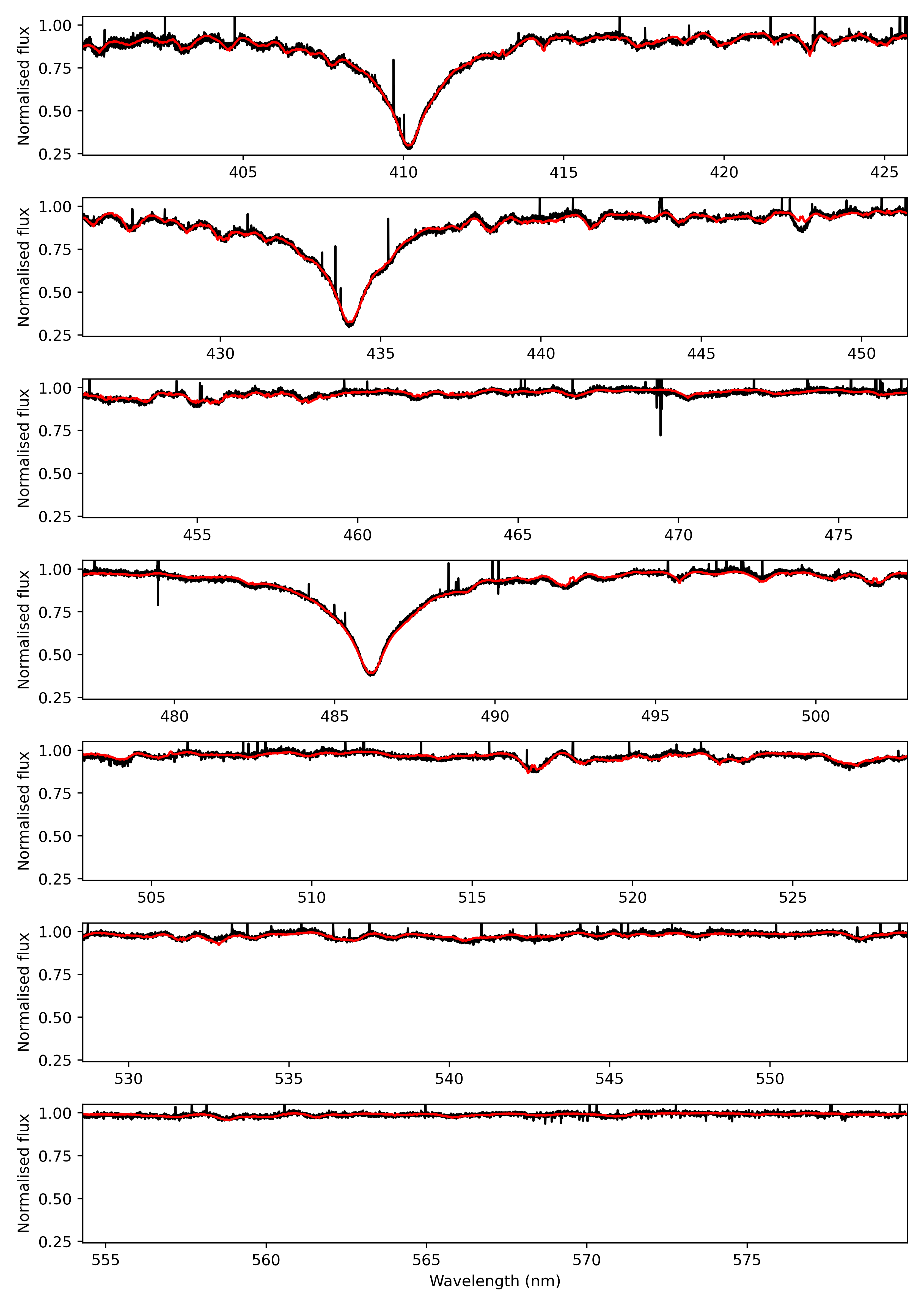
Figure 22: Spectrum of TIC 281582674 observed at 2023-03-16T02:04:10.433. The red line is the best-fitting theoretical spectrum.

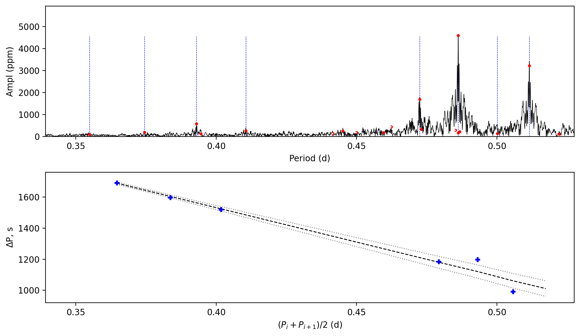
Figure 23: Period spacing pattern(s) of TIC 308307454. Top: amplitude spectrum as a function of period. Red dots are the peaks from the prewhitening process. Vertical lines mark the identified modes. Bottom: period spacing as a function of period. The black line is a linear fitting not the TAR fitting, and the grey lines exhibit the uncertainty region. The period is plotted as the mean value of the two consecutive peaks.

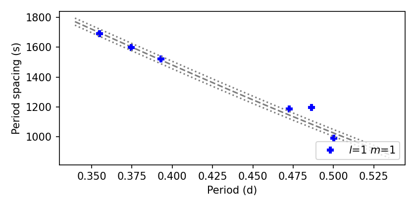
Figure 24: Period spacing pattern(s) from the TAR fitting of TIC 308307454. The dashed line marks the best-fitting model while the dotted lines exhibit the uncertainty region.

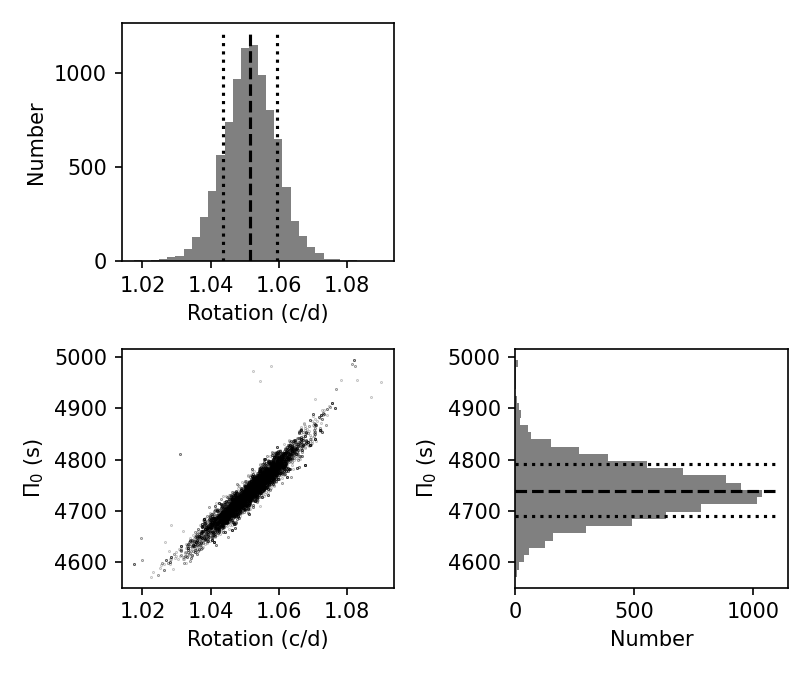
Figure 25: Posterior distributions of the TAR fitting of TIC 308307454.

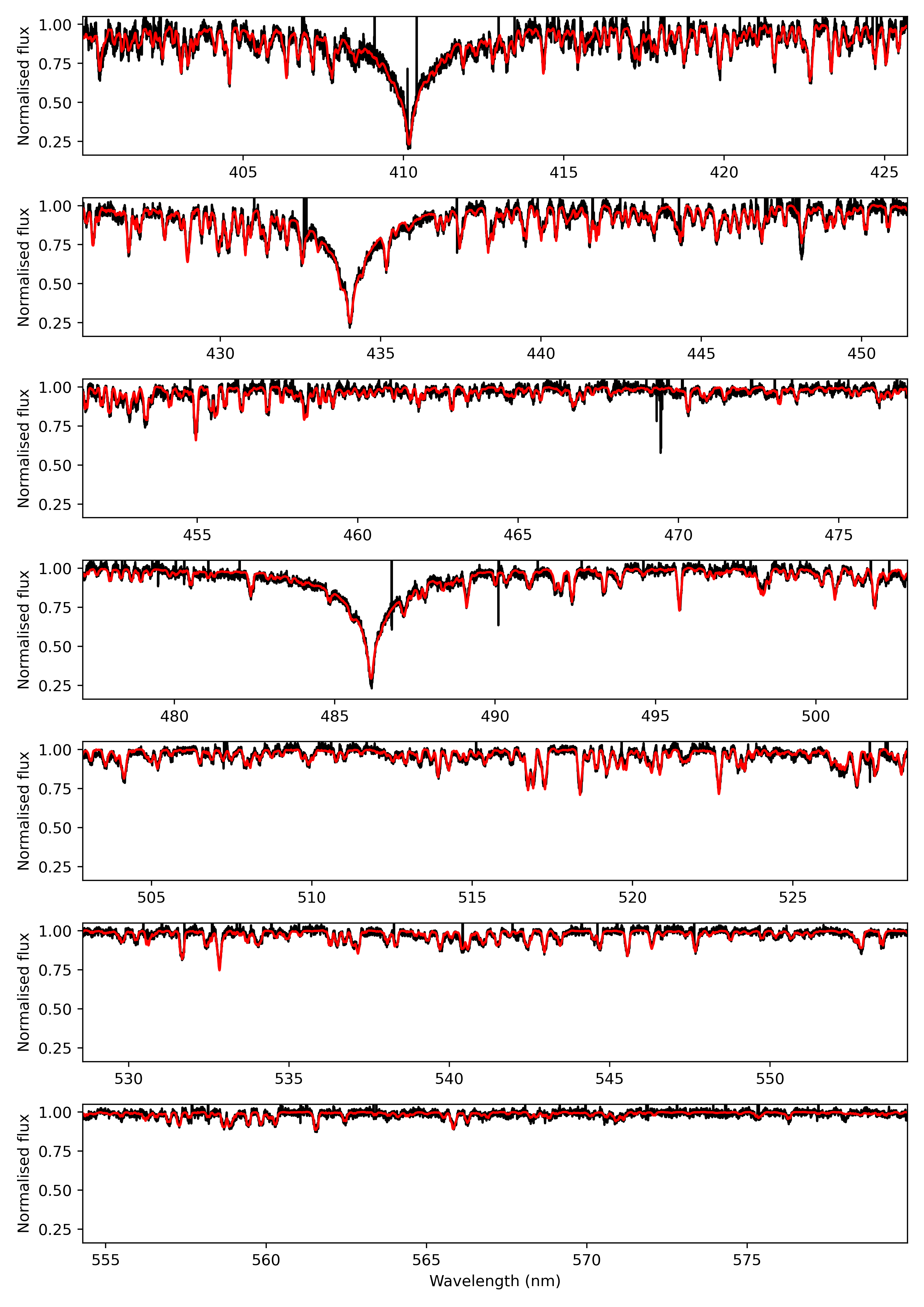
Figure 26: Spectrum of TIC 308307454 observed at 2023-03-13T00:54:35.517. The red line is the best-fitting theoretical spectrum.

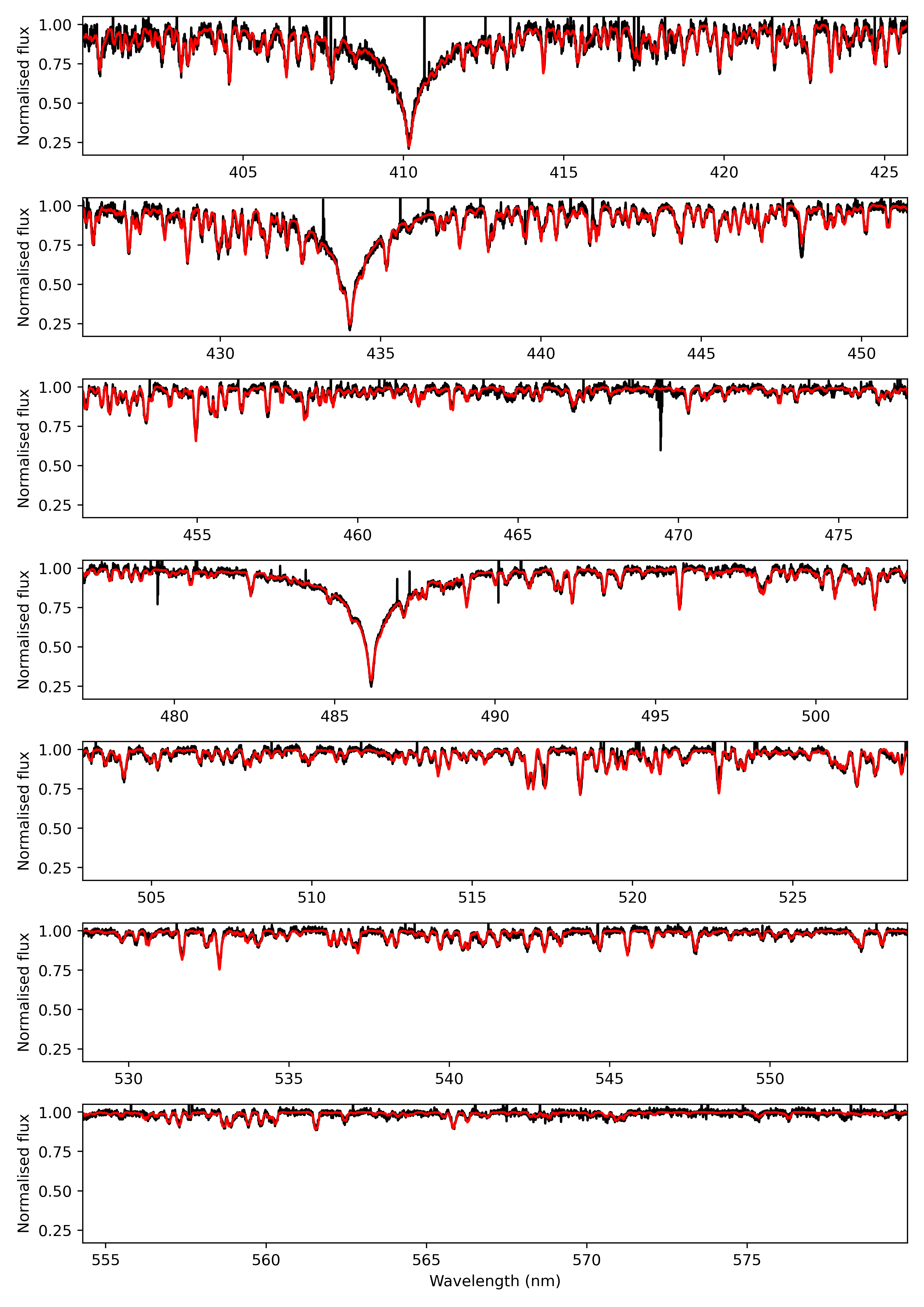
Figure 27: Spectrum of TIC 308307454 observed at 2023-03-14T04:55:16.136. The red line is the best-fitting theoretical spectrum.

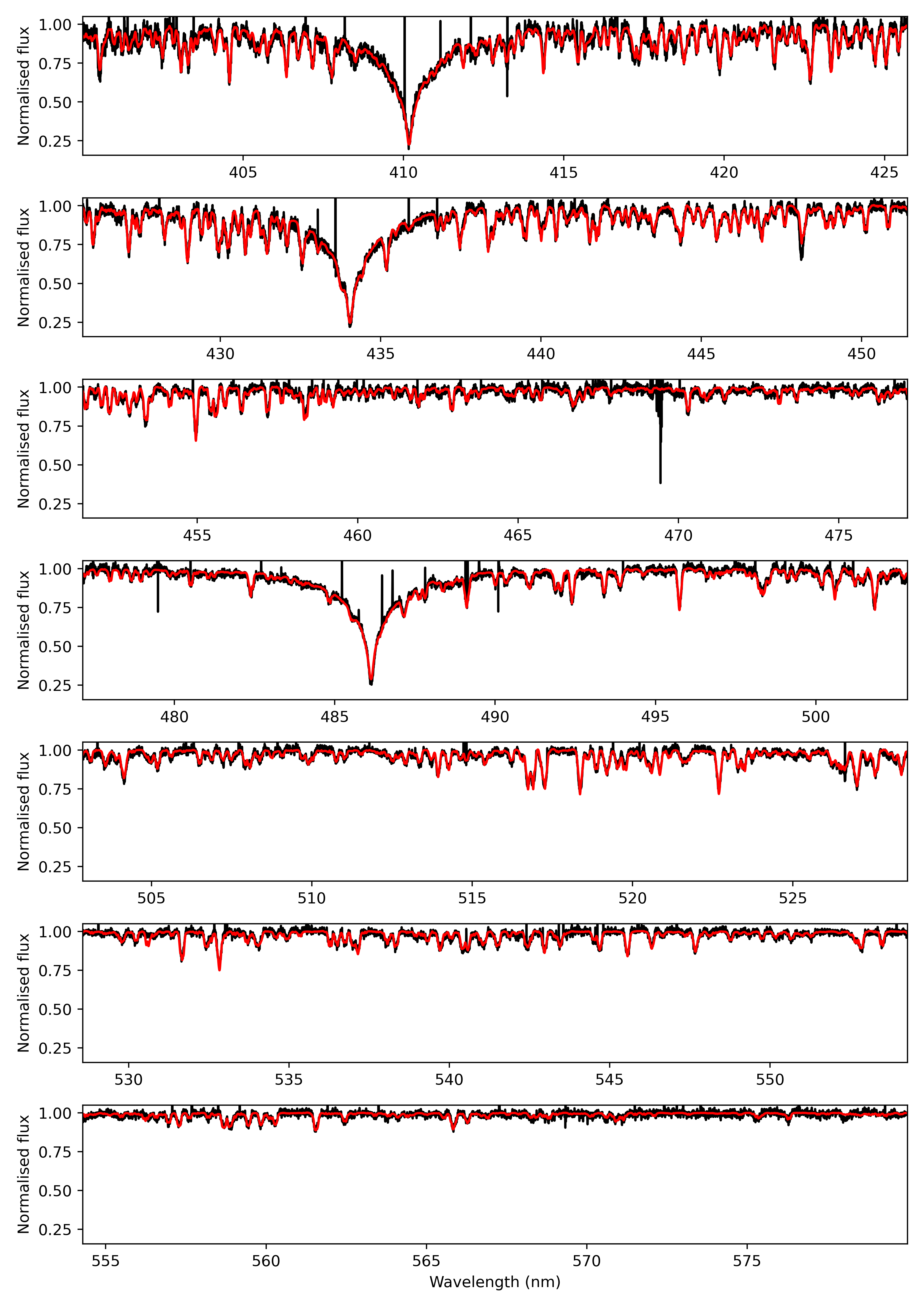
Figure 28: Spectrum of TIC 308307454 observed at 2023-03-16T03:13:33.242. The red line is the best-fitting theoretical spectrum.

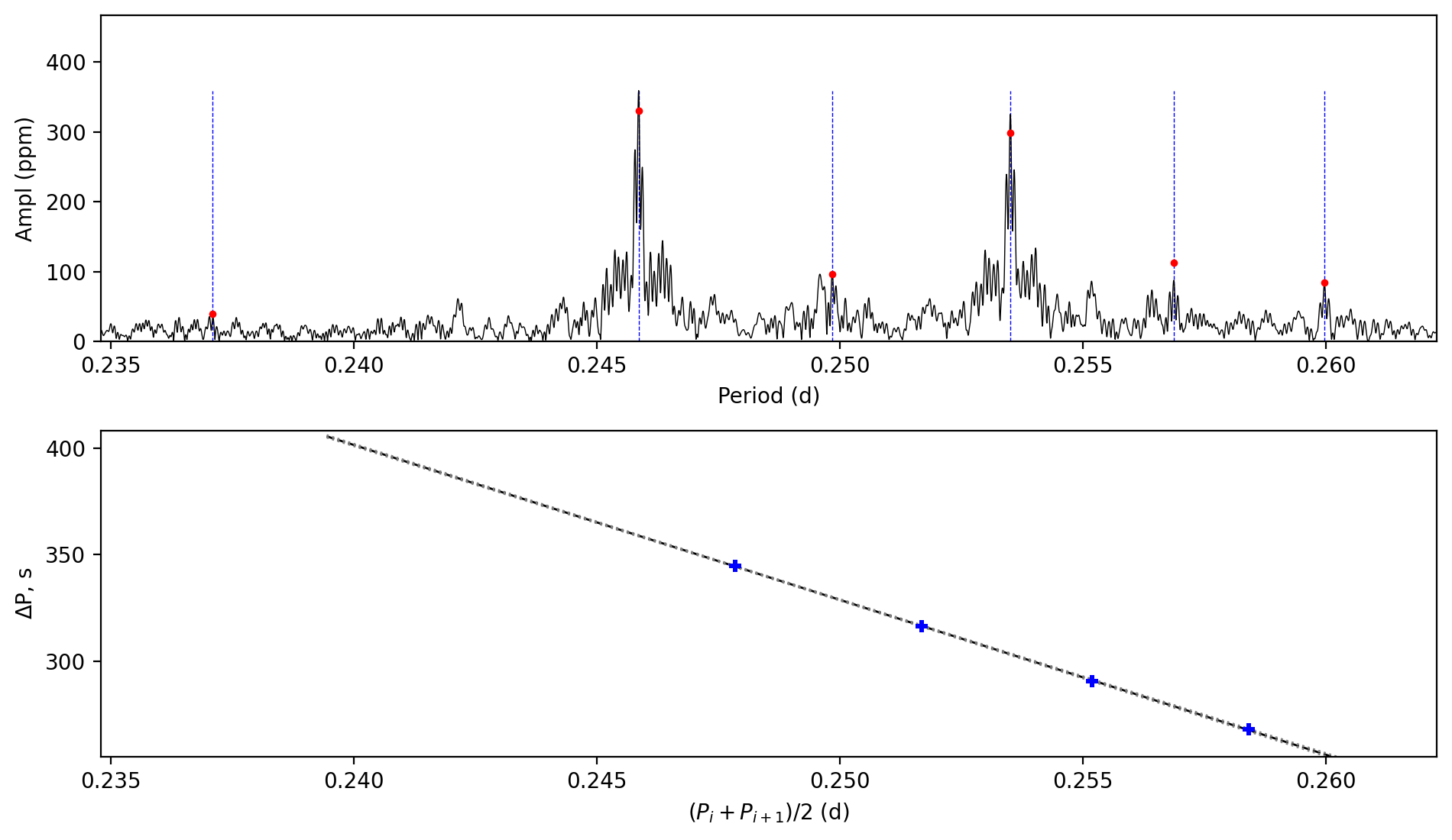
Figure 29: Period spacing pattern(s) of TIC 308992761. Top: amplitude spectrum as a function of period. Red dots are the peaks from the prewhitening process. Vertical lines mark the identified modes. Bottom: period spacing as a function of period. The black line is a linear fitting not the TAR fitting, and the grey lines exhibit the uncertainty region. The period is plotted as the mean value of the two consecutive peaks.

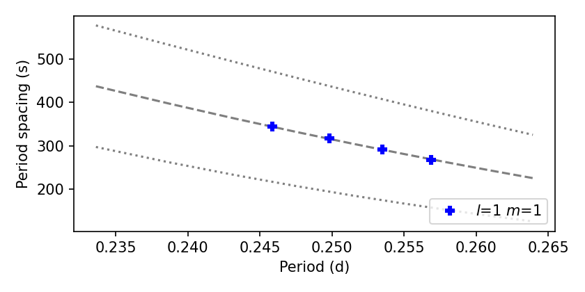
Figure 30: Period spacing pattern(s) from the TAR fitting of TIC 308992761. The dashed line marks the best-fitting model while the dotted lines exhibit the uncertainty region.

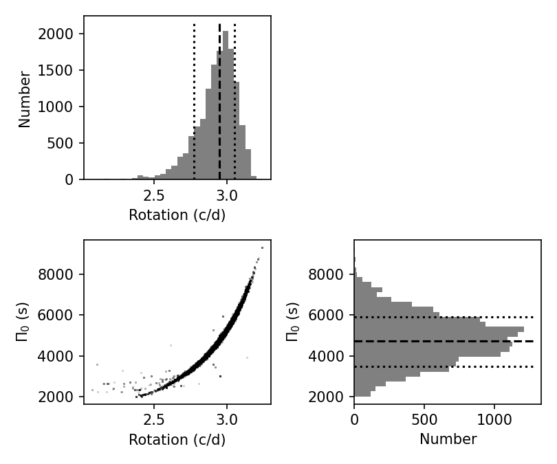
Figure 31: Posterior distributions of the TAR fitting of TIC 308992761.

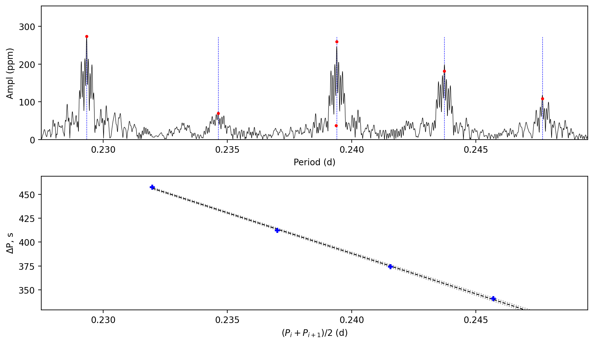
Figure 32: Period spacing pattern(s) of TIC 341043961. Top: amplitude spectrum as a function of period. Red dots are the peaks from the prewhitening process. Vertical lines mark the identified modes. Bottom: period spacing as a function of period. The black line is a linear fitting not the TAR fitting, and the grey lines exhibit the uncertainty region. The period is plotted as the mean value of the two consecutive peaks.

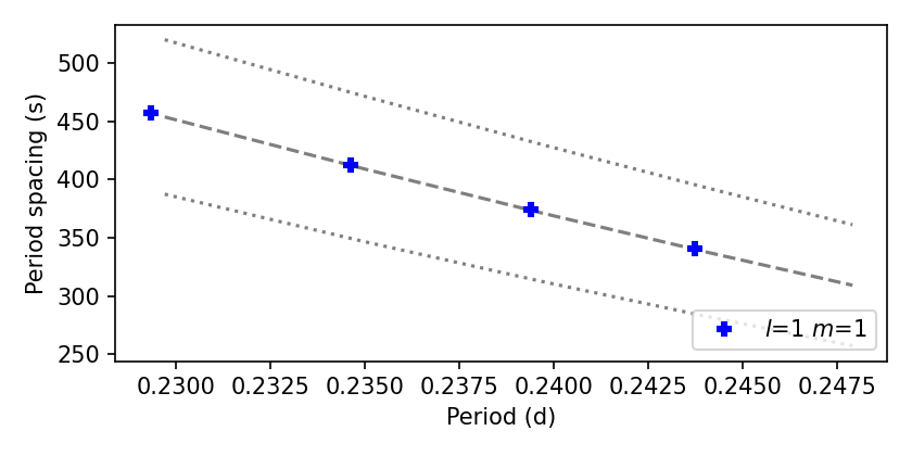
Figure 33: Period spacing pattern(s) from the TAR fitting of TIC 341043961. The dashed line marks the best-fitting model while the dotted lines exhibit the uncertainty region.

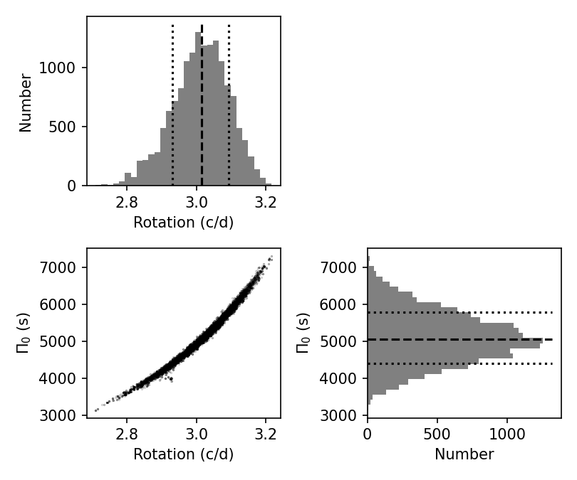
Figure 34: Posterior distributions of the TAR fitting of TIC 341043961.

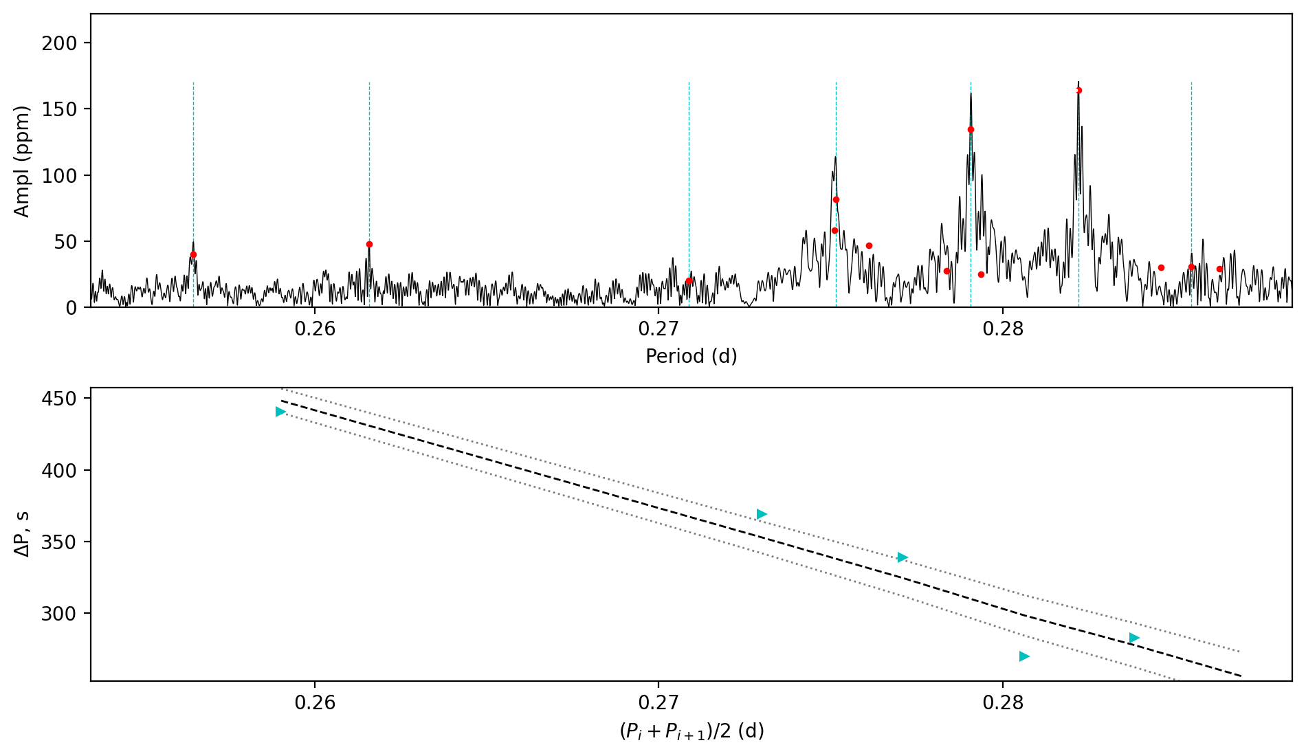
Figure 35: Period spacing pattern(s) of TIC 358466708. Top: amplitude spectrum as a function of period. Red dots are the peaks from the prewhitening process. Vertical lines mark the identified modes. Bottom: period spacing as a function of period. The black line is a linear fitting not the TAR fitting, and the grey lines exhibit the uncertainty region. The period is plotted as the mean value of the two consecutive peaks.

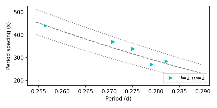
Figure 36: Period spacing pattern(s) from the TAR fitting of TIC 358466708. The dashed line marks the best-fitting model while the dotted lines exhibit the uncertainty region.

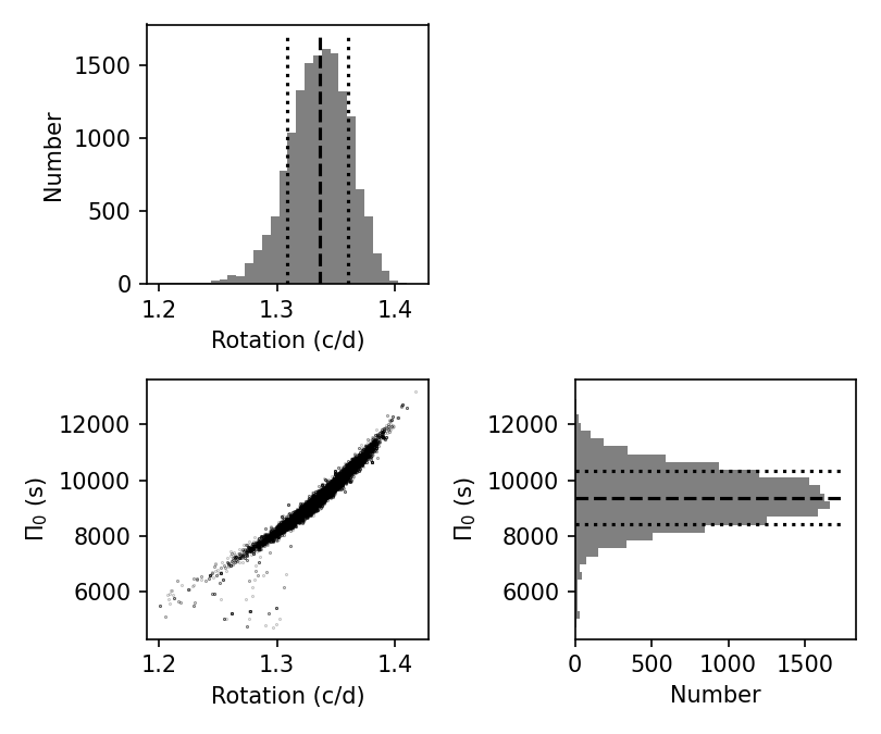
Figure 37: Posterior distributions of the TAR fitting of TIC 358466708.

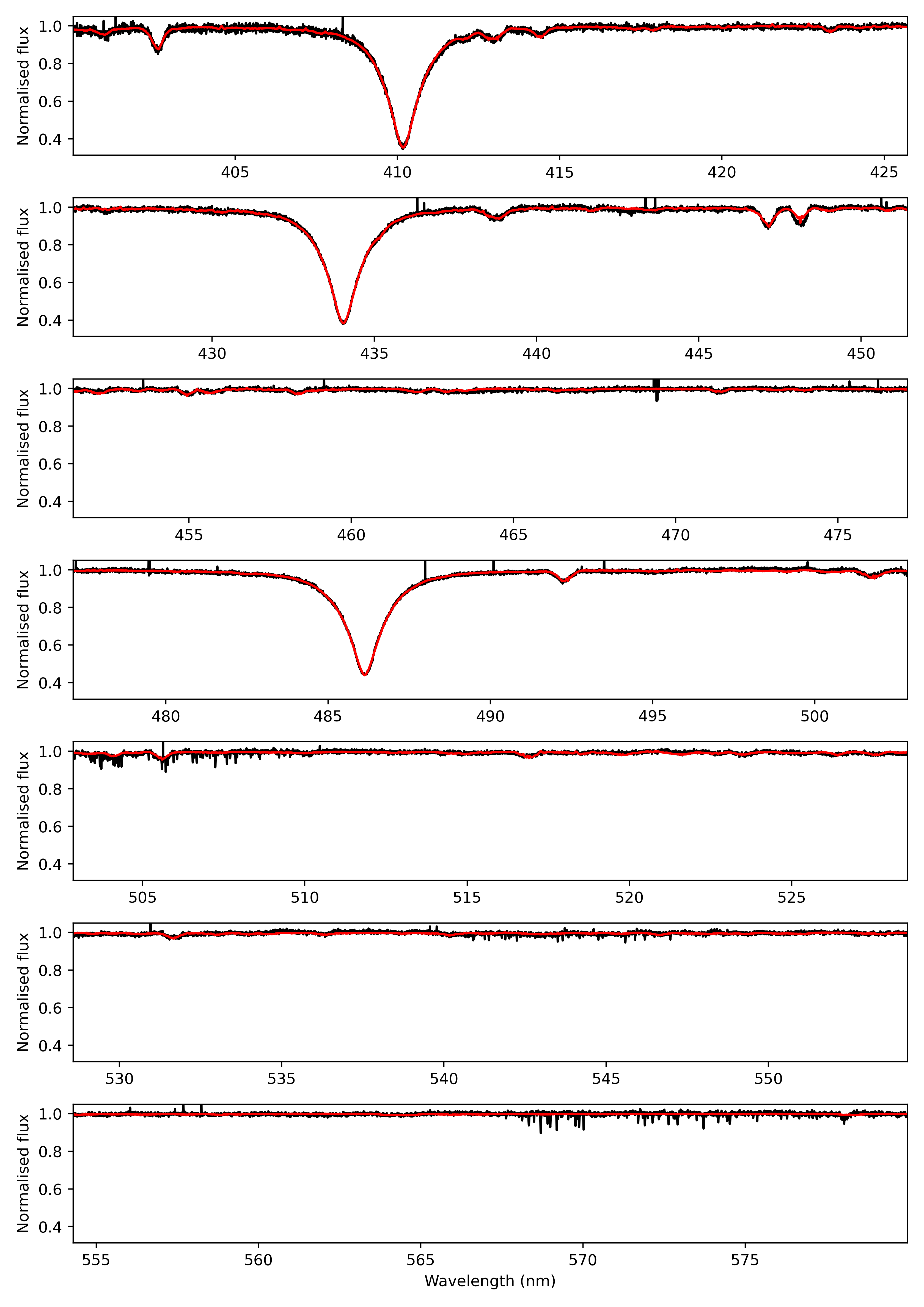
Figure 38: Spectrum of TIC 358466708 observed at 2023-03-12T06:45:37.221. The red line is the best-fitting theoretical spectrum.

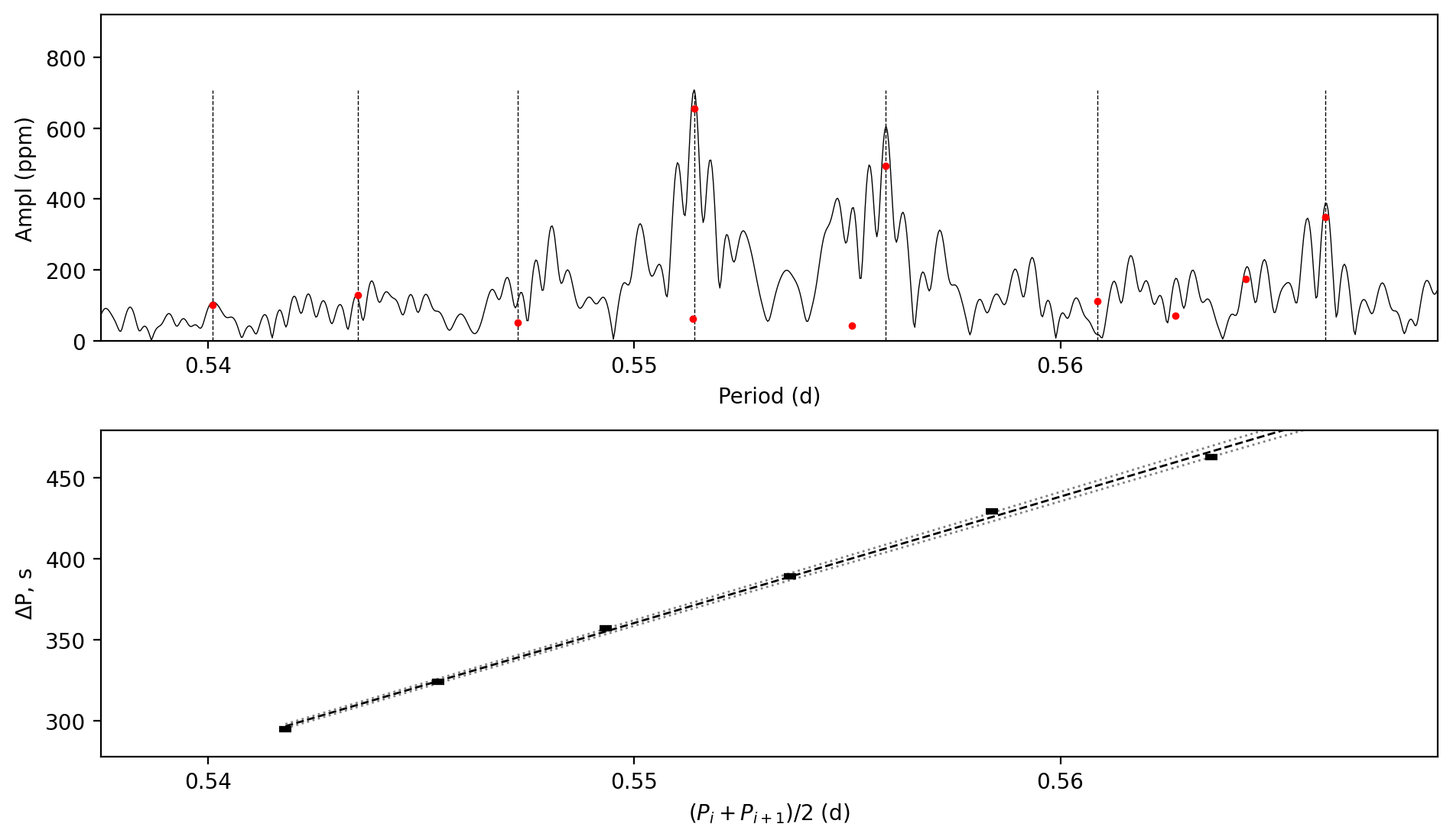
Figure 39: Period spacing pattern(s) of TIC 358466729. Top: amplitude spectrum as a function of period. Red dots are the peaks from the prewhitening process. Vertical lines mark the identified modes. Bottom: period spacing as a function of period. The black line is a linear fitting not the TAR fitting, and the grey lines exhibit the uncertainty region. The period is plotted as the mean value of the two consecutive peaks.

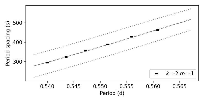
Figure 40: Period spacing pattern(s) from the TAR fitting of TIC 358466729. The dashed line marks the best-fitting model while the dotted lines exhibit the uncertainty region.

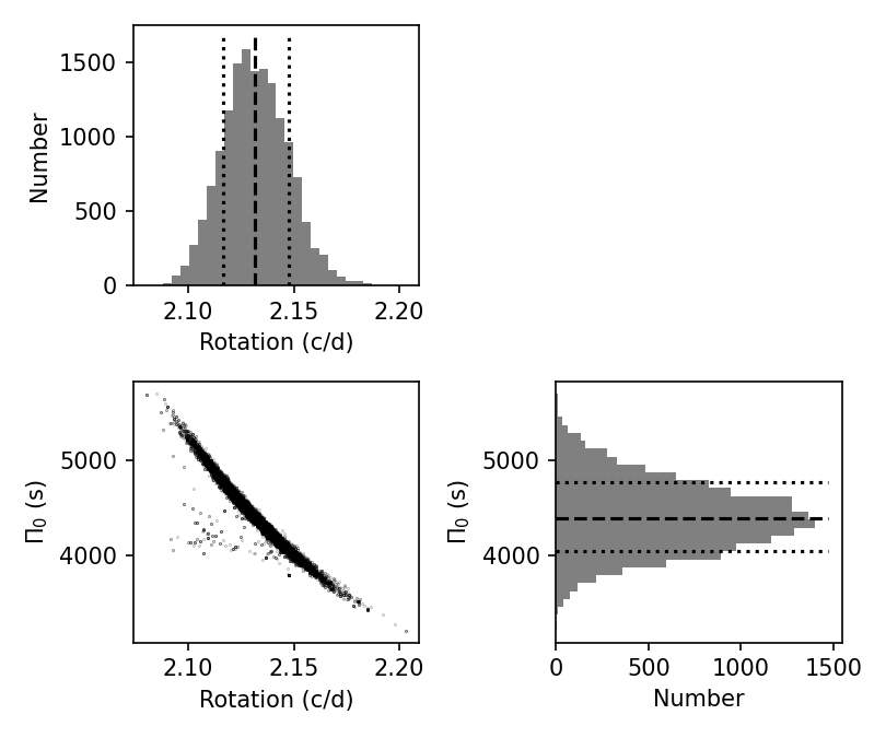
Figure 41: Posterior distributions of the TAR fitting of TIC 358466729.

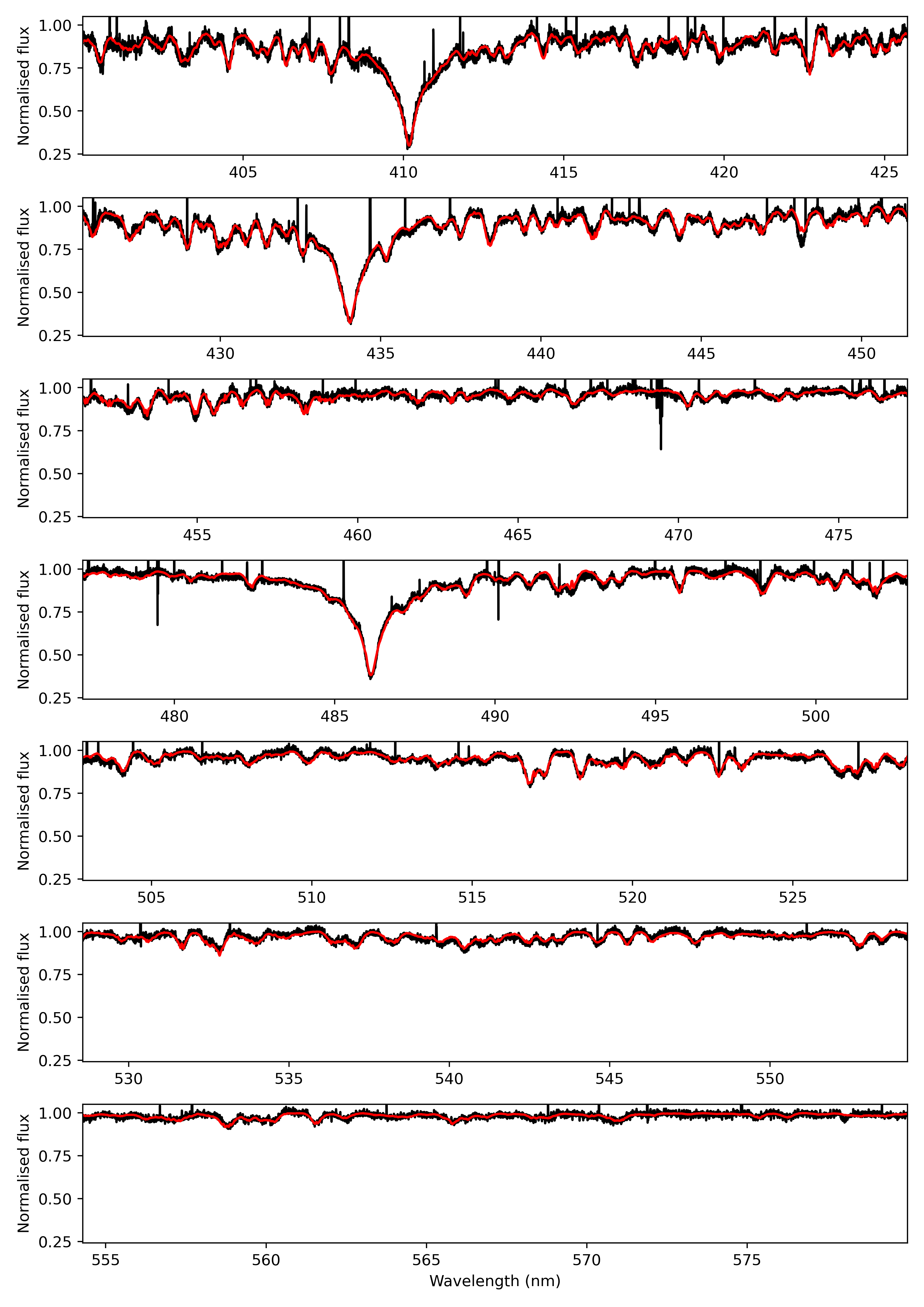
Figure 42: Spectrum of TIC 358466729 observed at 2023-03-13T02:48:18.645. The red line is the best-fitting theoretical spectrum.

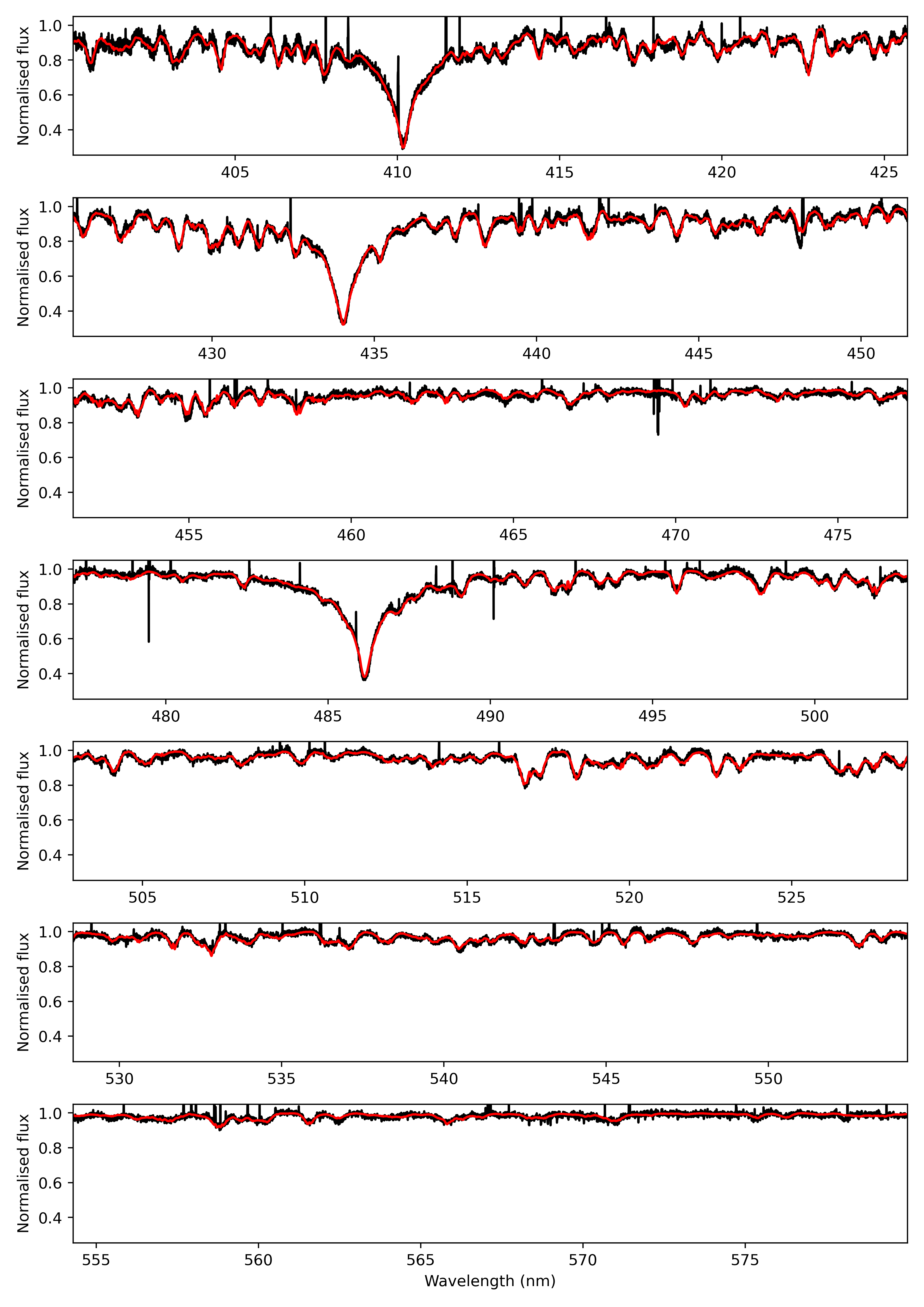
Figure 43: Spectrum of TIC 358466729 observed at 2023-03-15T02:09:35.139. The red line is the best-fitting theoretical spectrum.

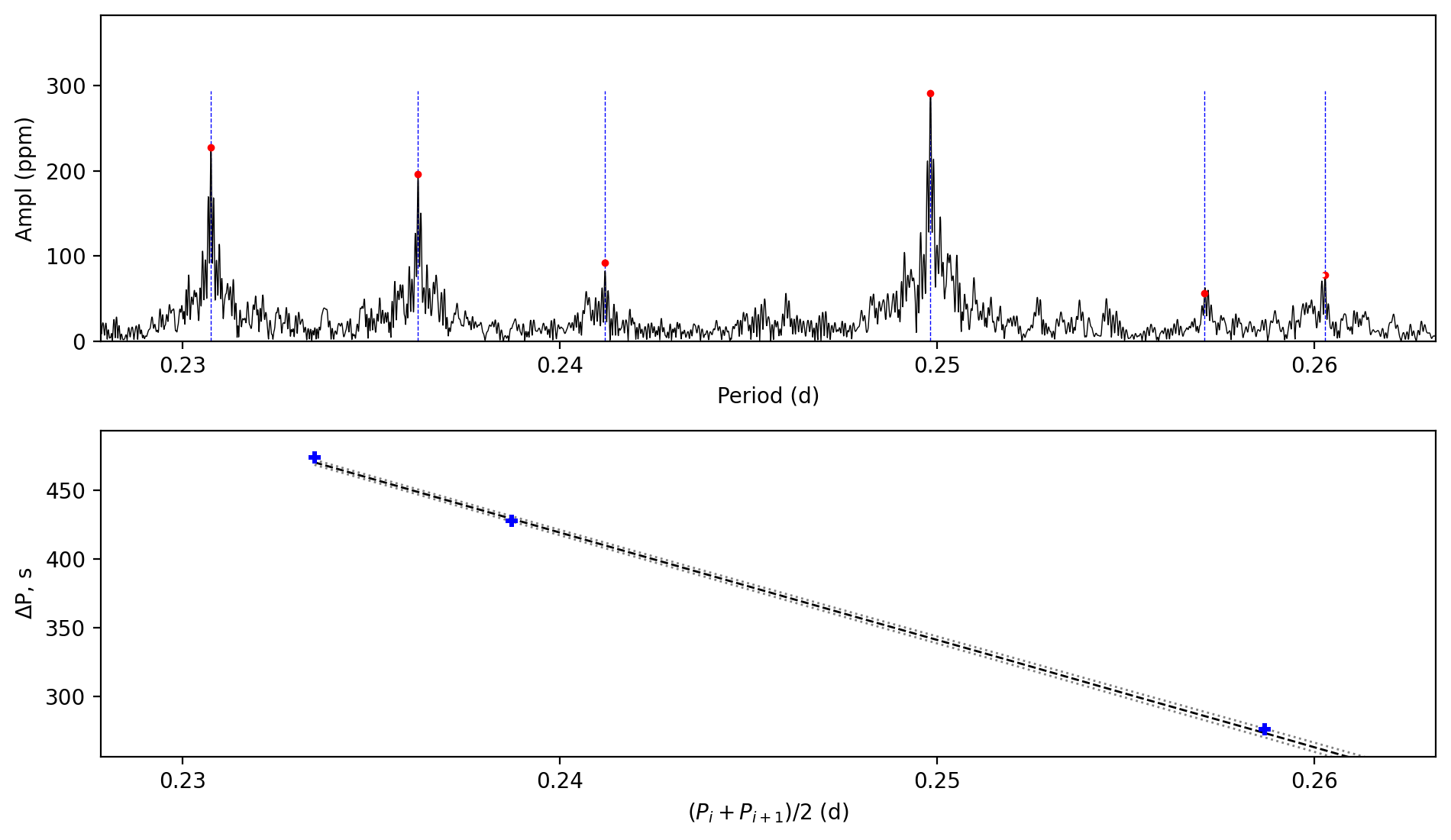
Figure 44: Period spacing pattern(s) of TIC 364398040. Top: amplitude spectrum as a function of period. Red dots are the peaks from the prewhitening process. Vertical lines mark the identified modes. Bottom: period spacing as a function of period. The black line is a linear fitting not the TAR fitting, and the grey lines exhibit the uncertainty region. The period is plotted as the mean value of the two consecutive peaks.

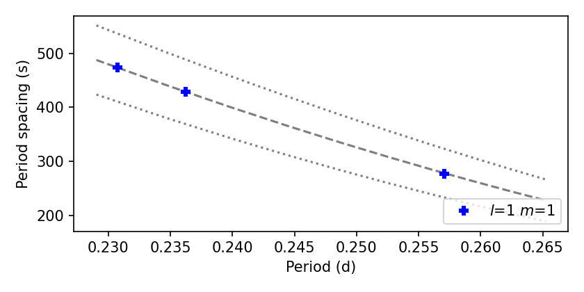
Figure 45: Period spacing pattern(s) from the TAR fitting of TIC 364398040. The dashed line marks the best-fitting model while the dotted lines exhibit the uncertainty region.

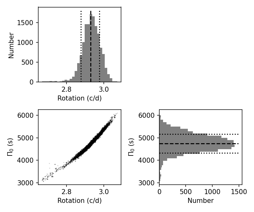
Figure 46: Posterior distributions of the TAR fitting of TIC 364398040.

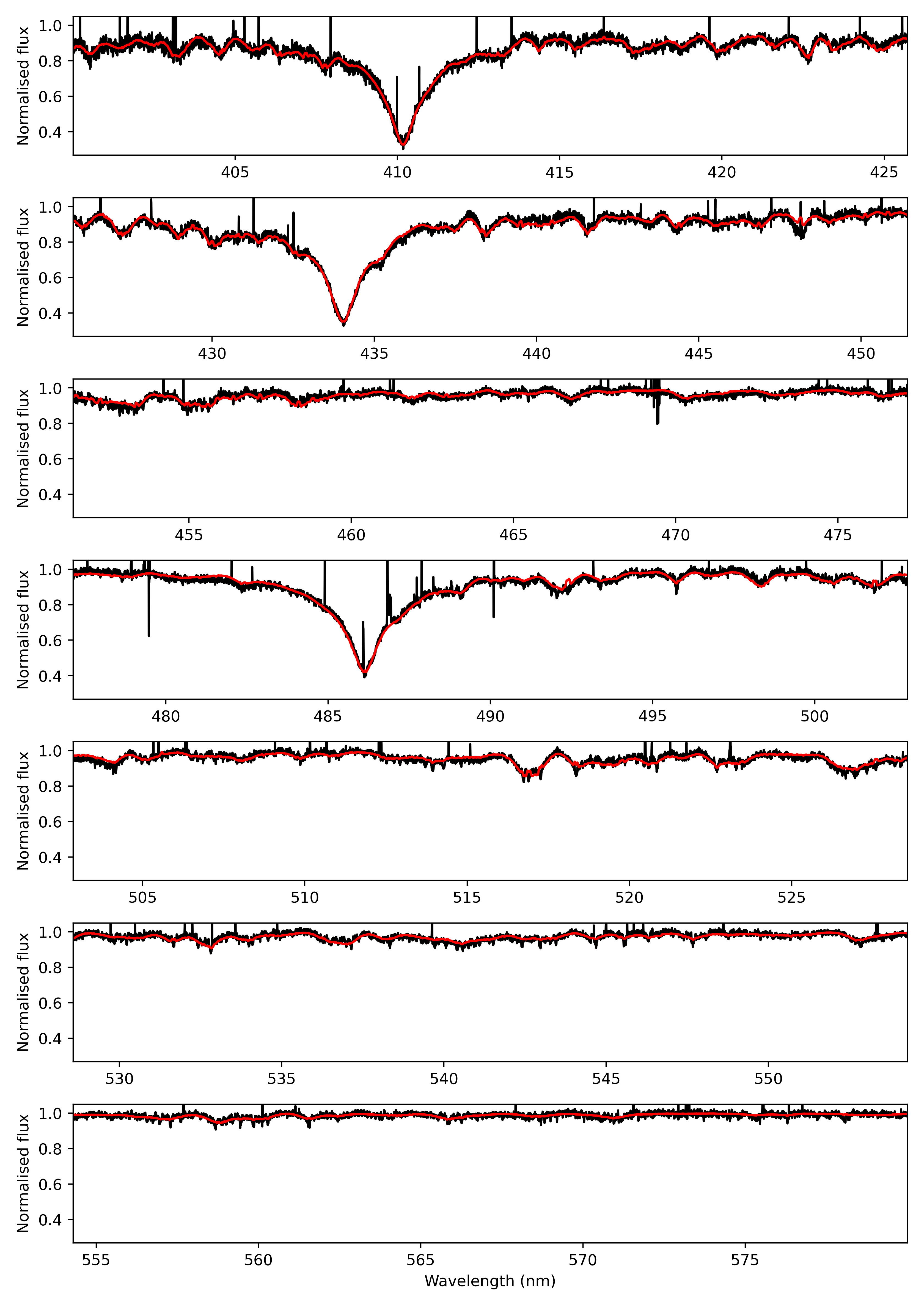
Figure 47: Spectrum of TIC 364398040 observed at 2023-03-13T00:20:15.606. The red line is the best-fitting theoretical spectrum.

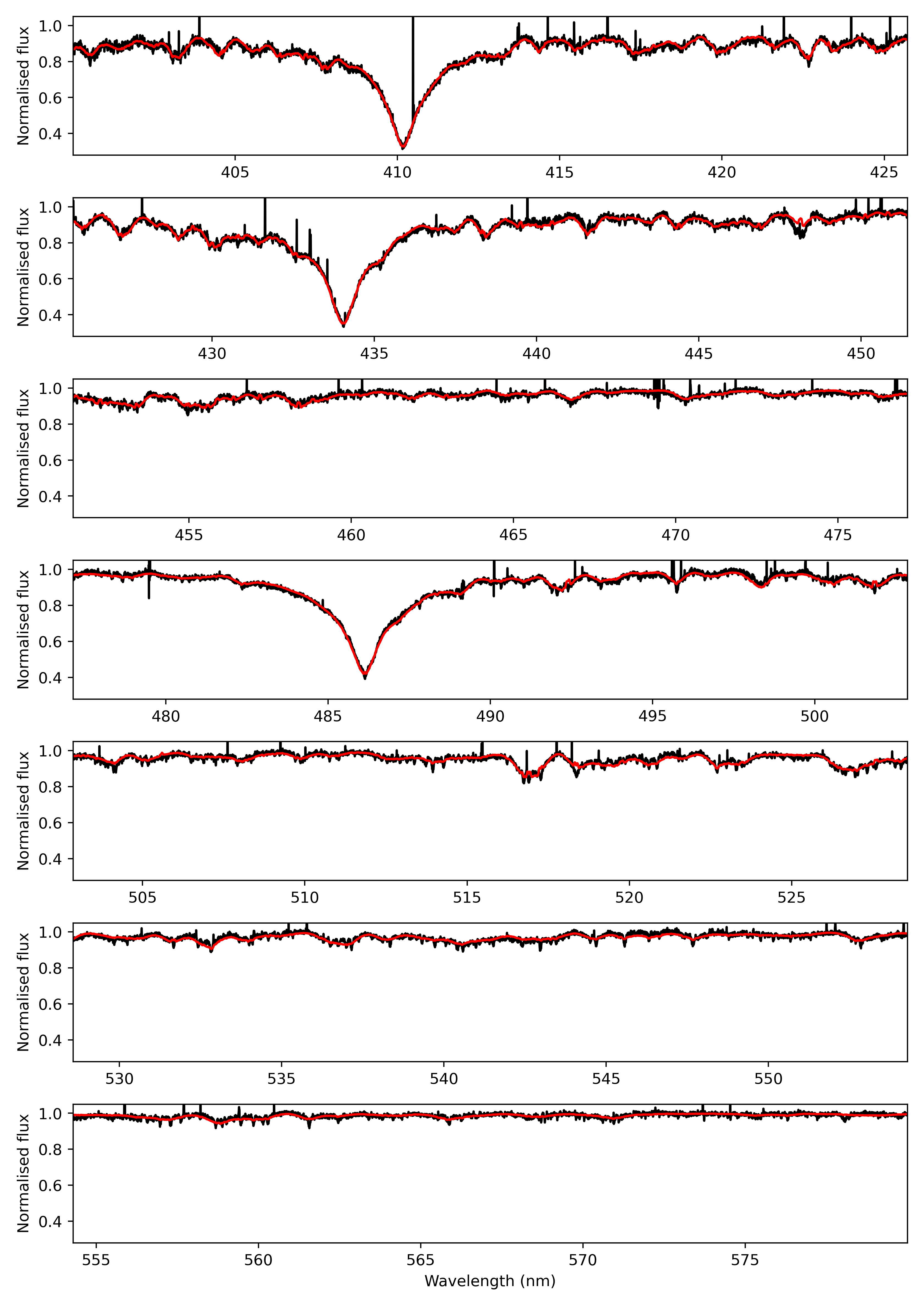
Figure 48: Spectrum of TIC 364398040 observed at 2023-03-15T01:33:49.149. The red line is the best-fitting theoretical spectrum.

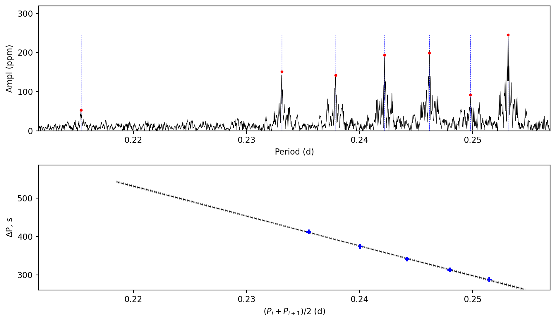
Figure 49: Period spacing pattern(s) of TIC 372912679. Top: amplitude spectrum as a function of period. Red dots are the peaks from the prewhitening process. Vertical lines mark the identified modes. Bottom: period spacing as a function of period. The black line is a linear fitting not the TAR fitting, and the grey lines exhibit the uncertainty region. The period is plotted as the mean value of the two consecutive peaks.

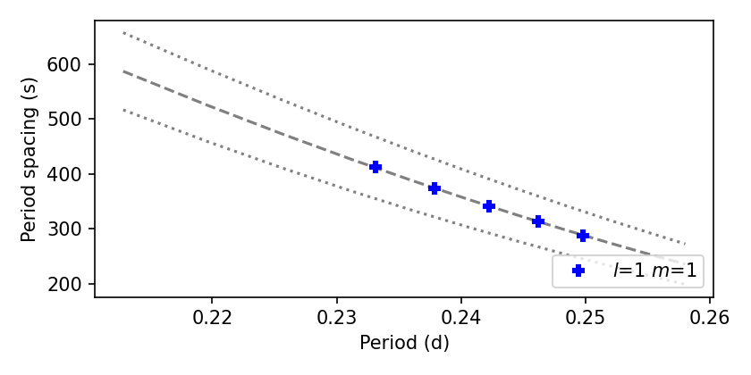
Figure 50: Period spacing pattern(s) from the TAR fitting of TIC 372912679. The dashed line marks the best-fitting model while the dotted lines exhibit the uncertainty region.

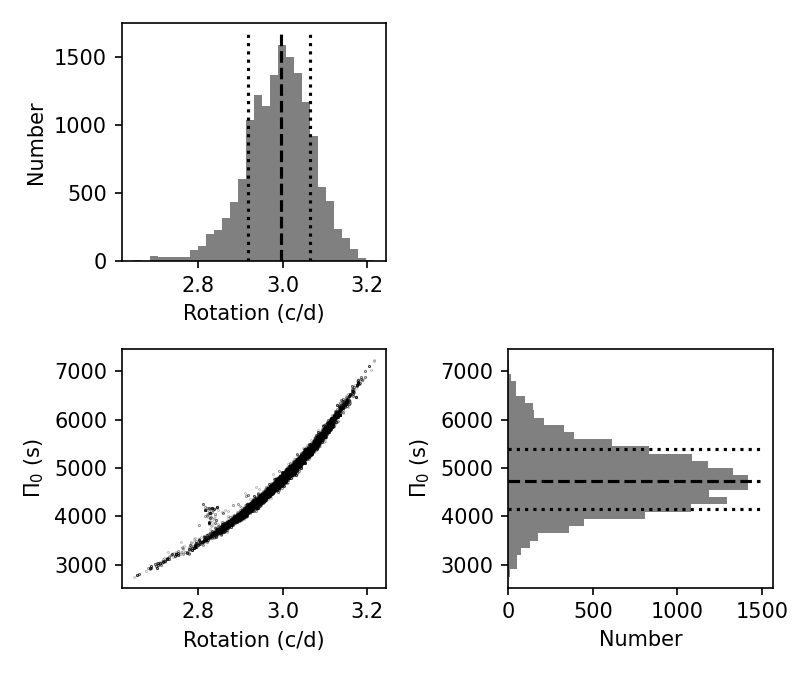
Figure 51: Posterior distributions of the TAR fitting of TIC 372912679.

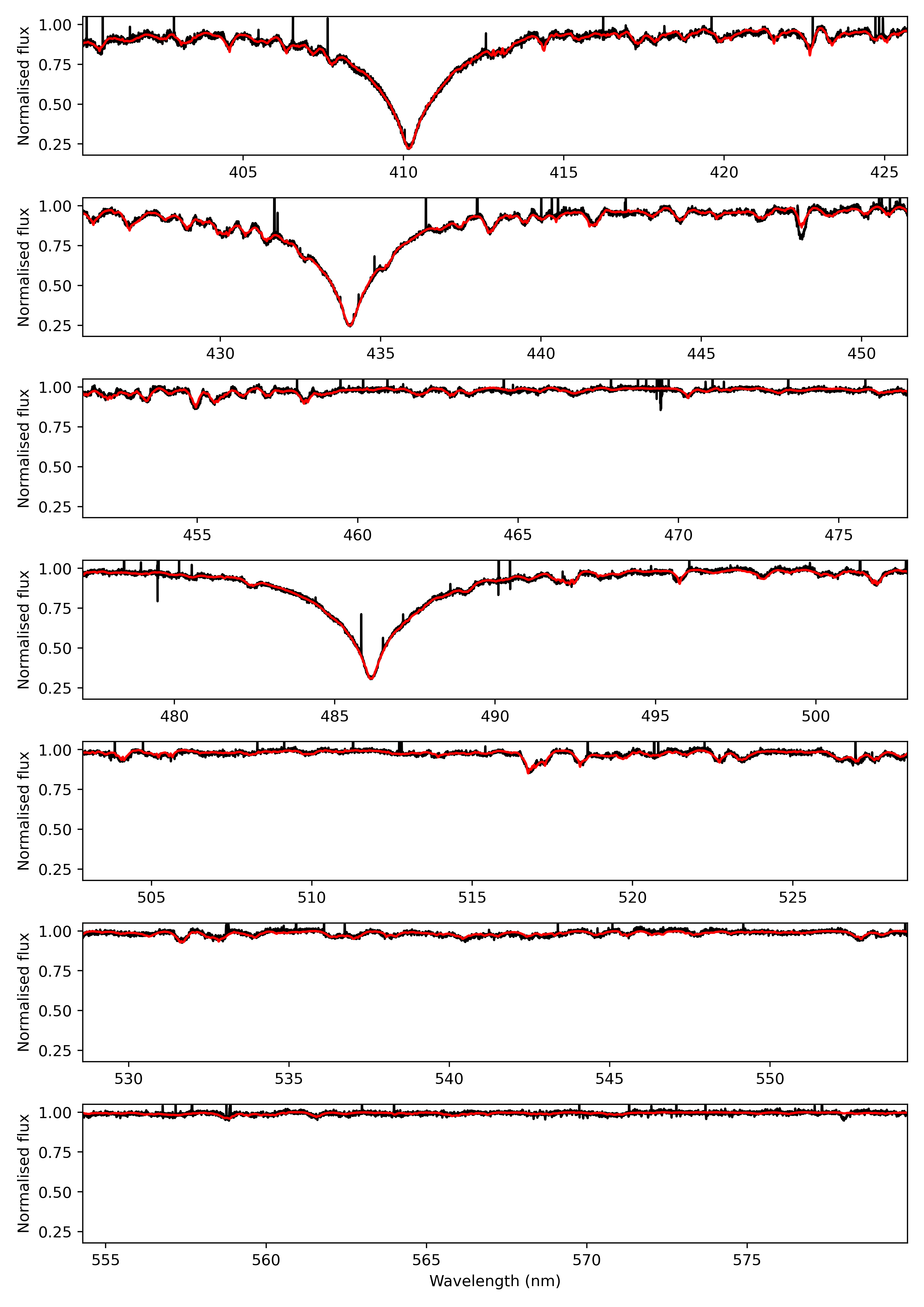
Figure 52: Spectrum of TIC 372912679 observed at 2023-03-14T01:48:11.434. The red line is the best-fitting theoretical spectrum.

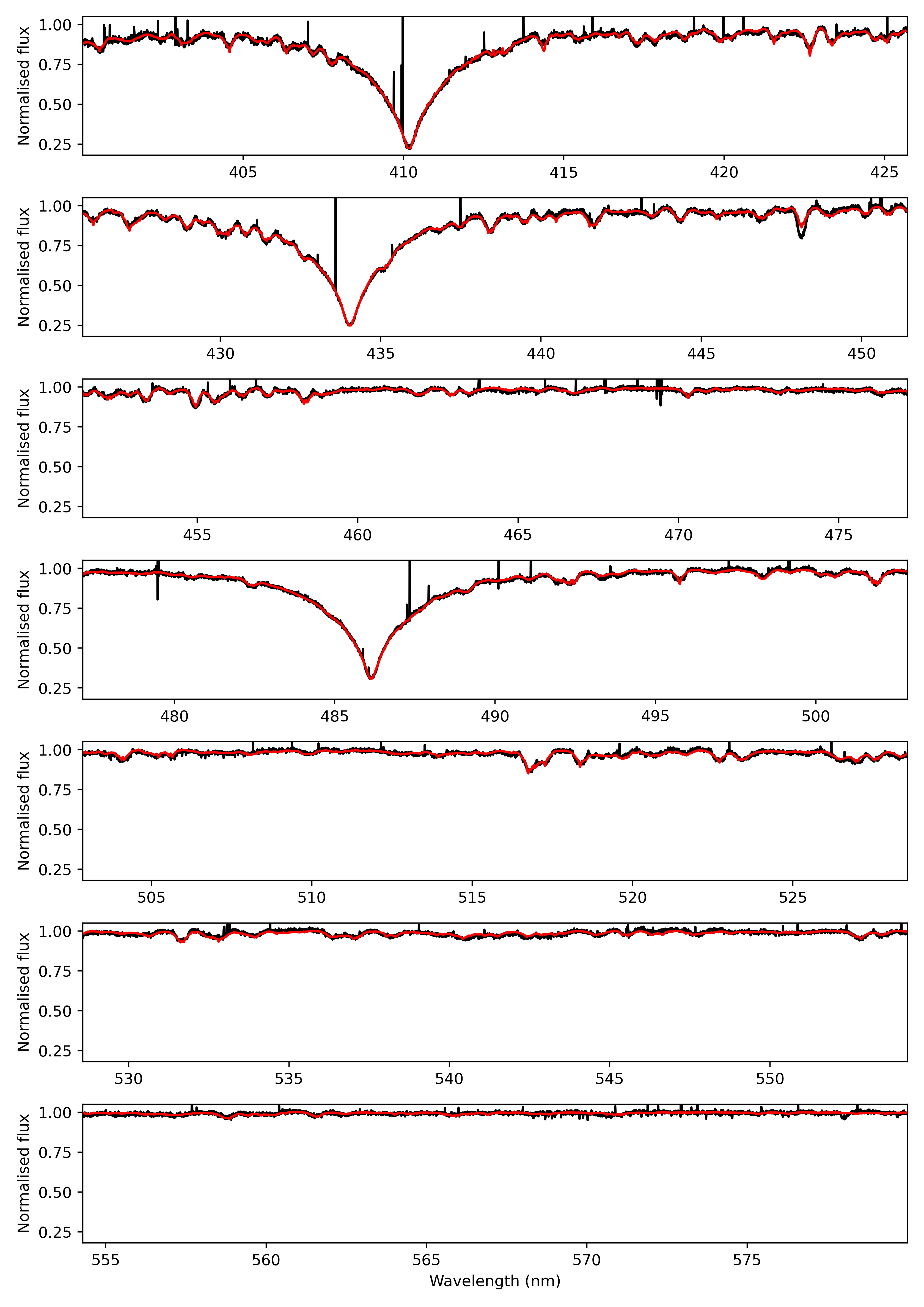
Figure 53: Spectrum of TIC 372912679 observed at 2023-03-15T01:01:24.311. The red line is the best-fitting theoretical spectrum.

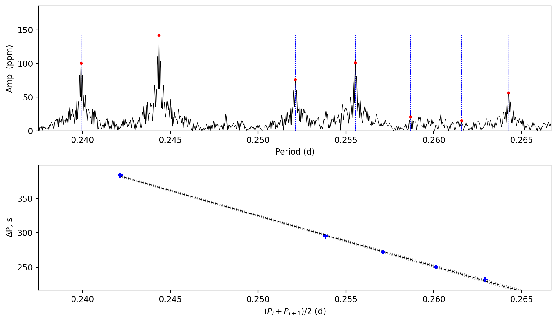
Figure 54: Period spacing pattern(s) of TIC 372913043. Top: amplitude spectrum as a function of period. Red dots are the peaks from the prewhitening process. Vertical lines mark the identified modes. Bottom: period spacing as a function of period. The black line is a linear fitting not the TAR fitting, and the grey lines exhibit the uncertainty region. The period is plotted as the mean value of the two consecutive peaks.

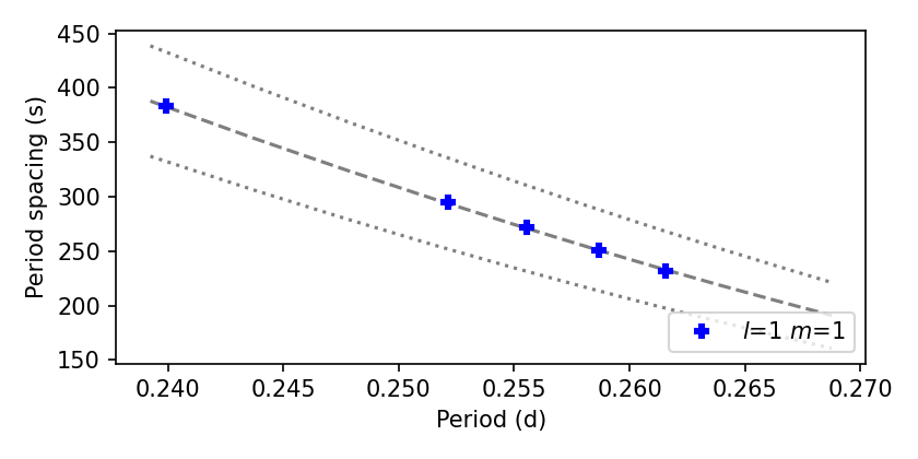
Figure 55: Period spacing pattern(s) from the TAR fitting of TIC 372913043. The dashed line marks the best-fitting model while the dotted lines exhibit the uncertainty region.

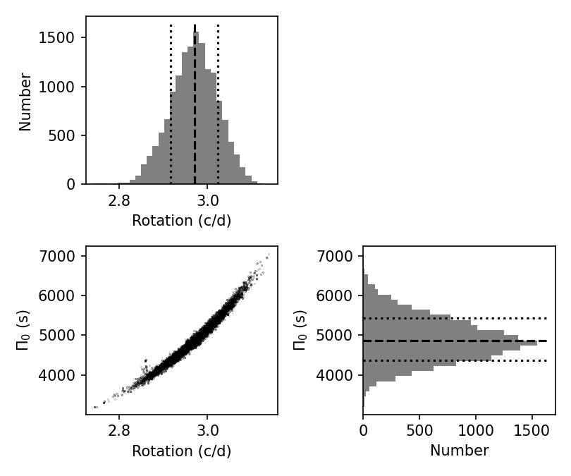
Figure 56: Posterior distributions of the TAR fitting of TIC 372913043.

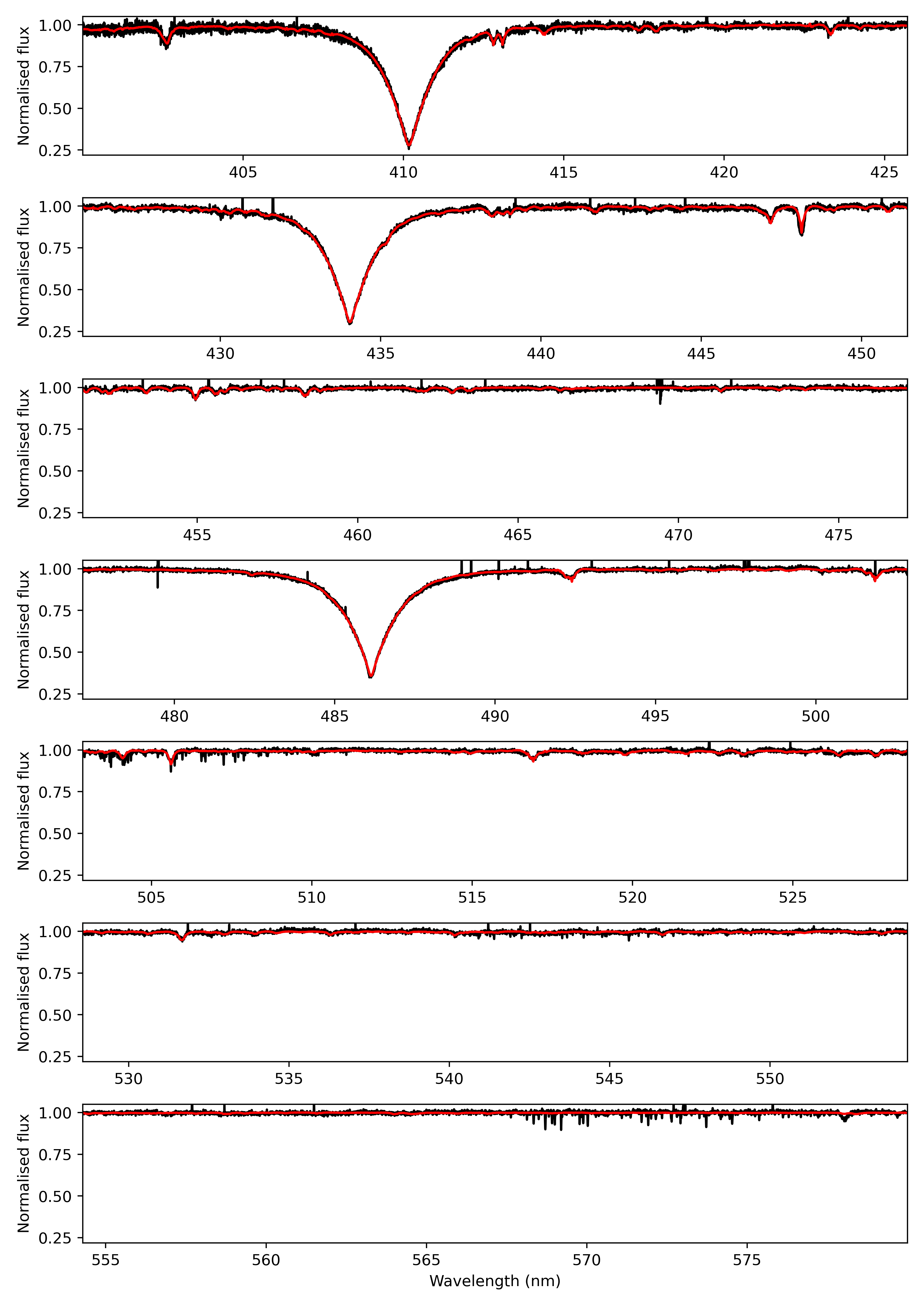
Figure 57: Spectrum of TIC 372913043 observed at 2023-03-12T06:59:31.142. The red line is the best-fitting theoretical spectrum.

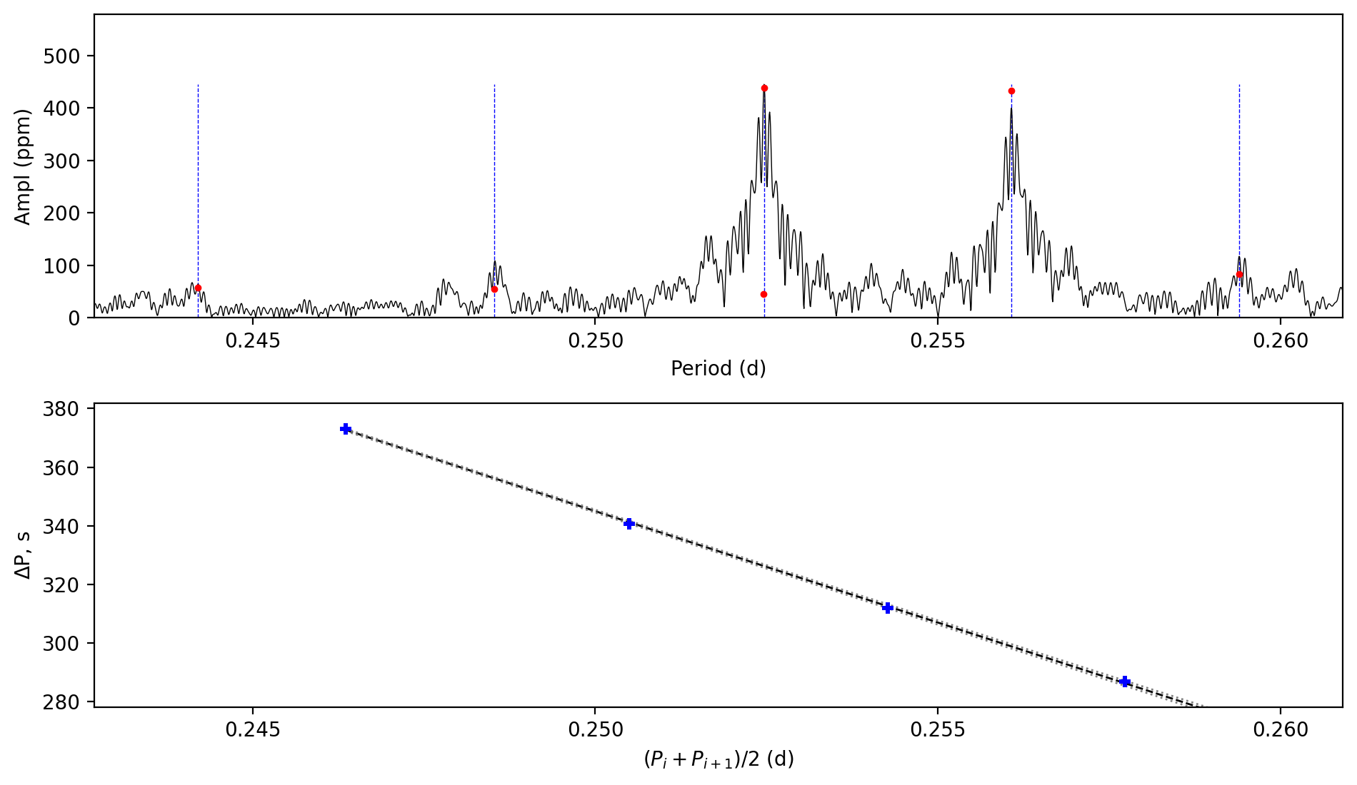
Figure 58: Period spacing pattern(s) of TIC 410451583. Top: amplitude spectrum as a function of period. Red dots are the peaks from the prewhitening process. Vertical lines mark the identified modes. Bottom: period spacing as a function of period. The black line is a linear fitting not the TAR fitting, and the grey lines exhibit the uncertainty region. The period is plotted as the mean value of the two consecutive peaks.

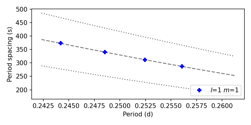
Figure 59: Period spacing pattern(s) from the TAR fitting of TIC 410451583. The dashed line marks the best-fitting model while the dotted lines exhibit the uncertainty region.

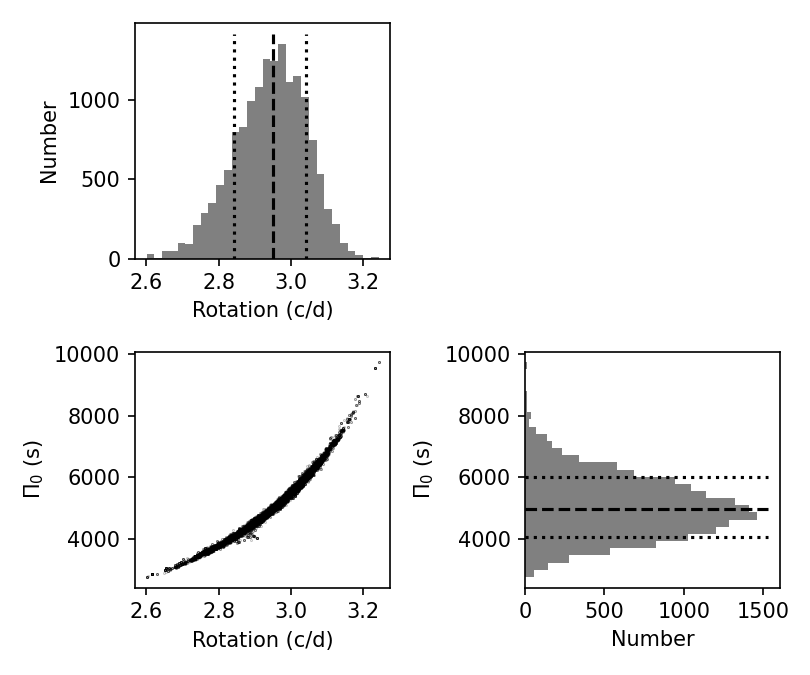
Figure 60: Posterior distributions of the TAR fitting of TIC 410451583.

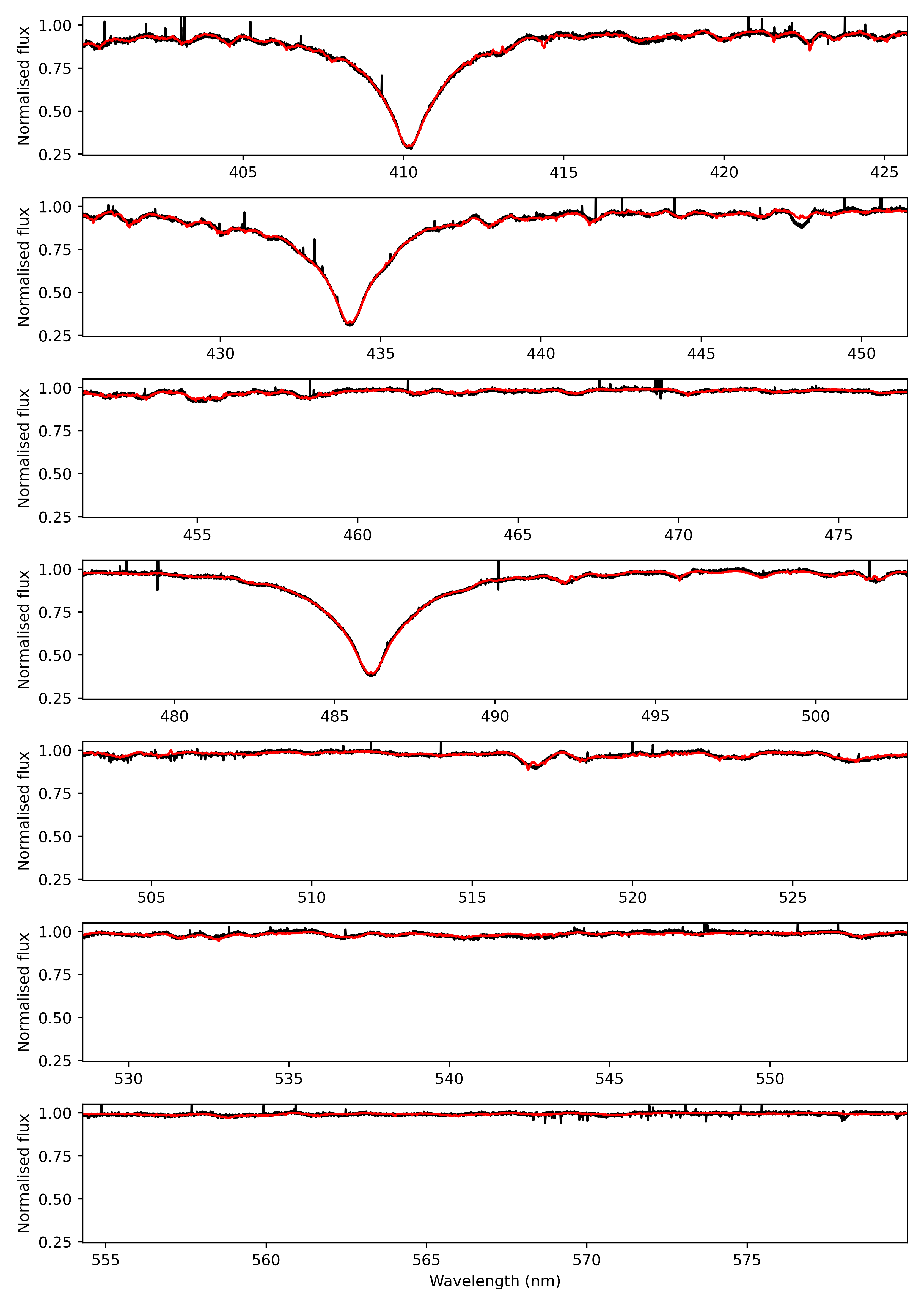
Figure 61: Spectrum of TIC 410451583 observed at 2023-03-14T04:21:29.958. The red line is the best-fitting theoretical spectrum.

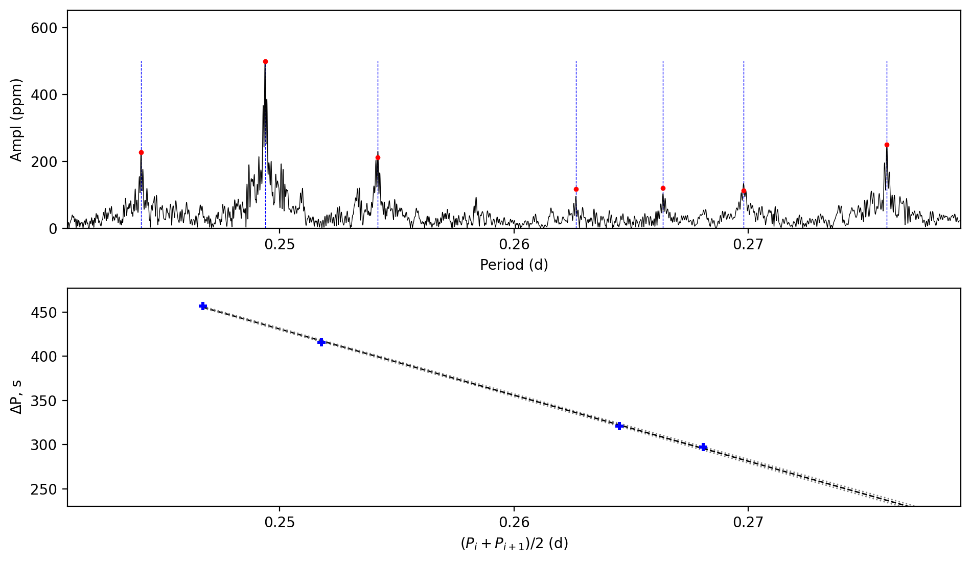
Figure 62: Period spacing pattern(s) of TIC 410452218. Top: amplitude spectrum as a function of period. Red dots are the peaks from the prewhitening process. Vertical lines mark the identified modes. Bottom: period spacing as a function of period. The black line is a linear fitting not the TAR fitting, and the grey lines exhibit the uncertainty region. The period is plotted as the mean value of the two consecutive peaks.

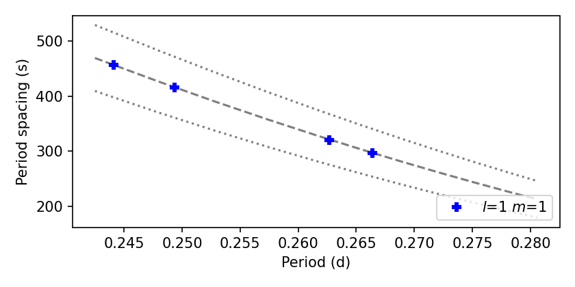
Figure 63: Period spacing pattern(s) from the TAR fitting of TIC 410452218. The dashed line marks the best-fitting model while the dotted lines exhibit the uncertainty region.

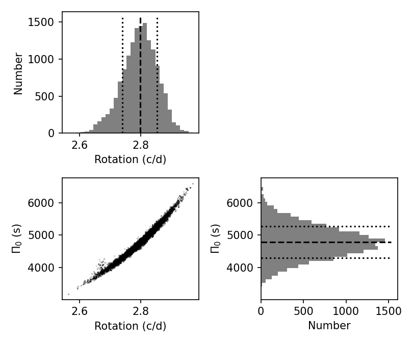
Figure 64: Posterior distributions of the TAR fitting of TIC 410452218.

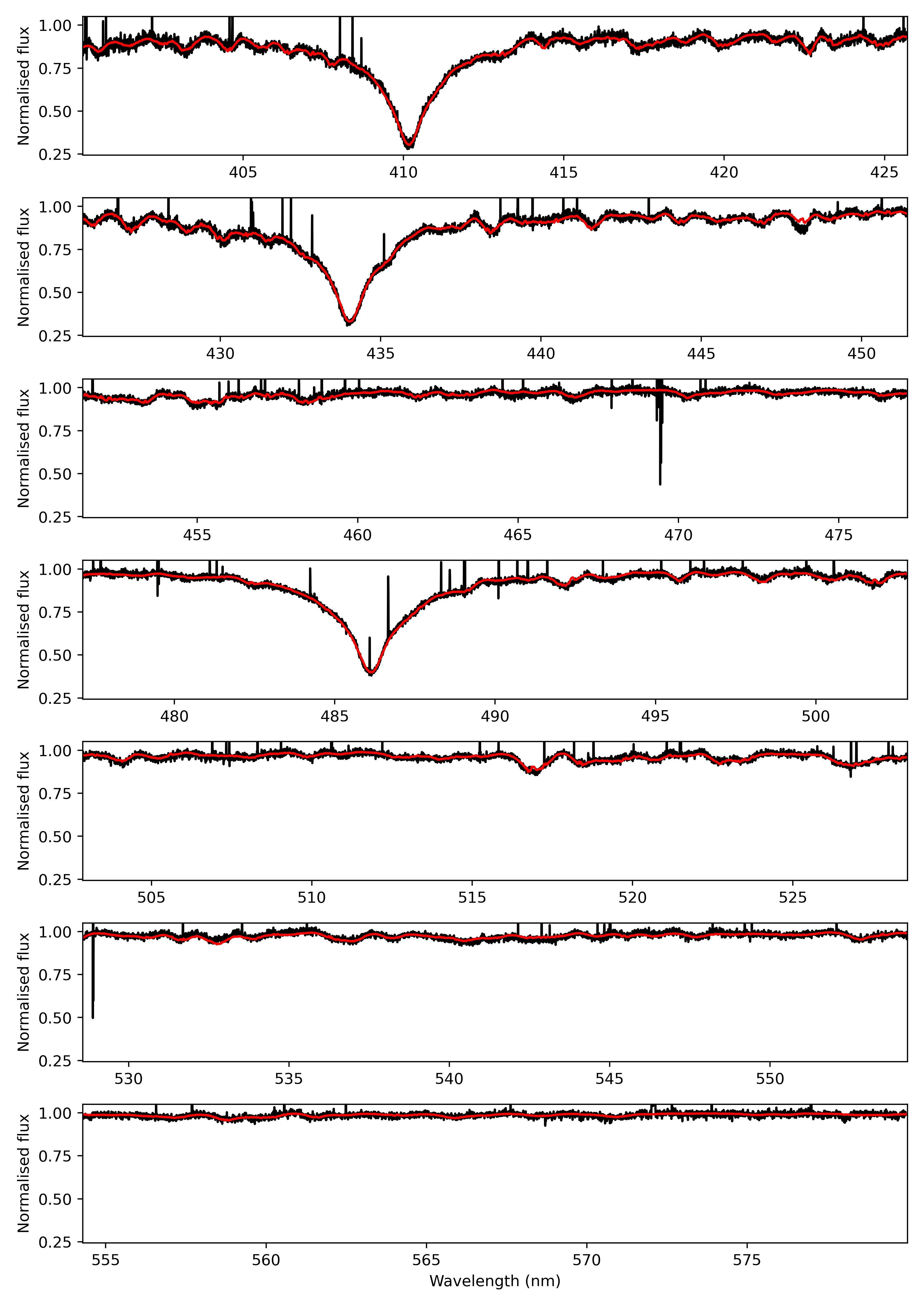
Figure 65: Spectrum of TIC 410452218 observed at 2023-03-14T02:24:11.888. The red line is the best-fitting theoretical spectrum.

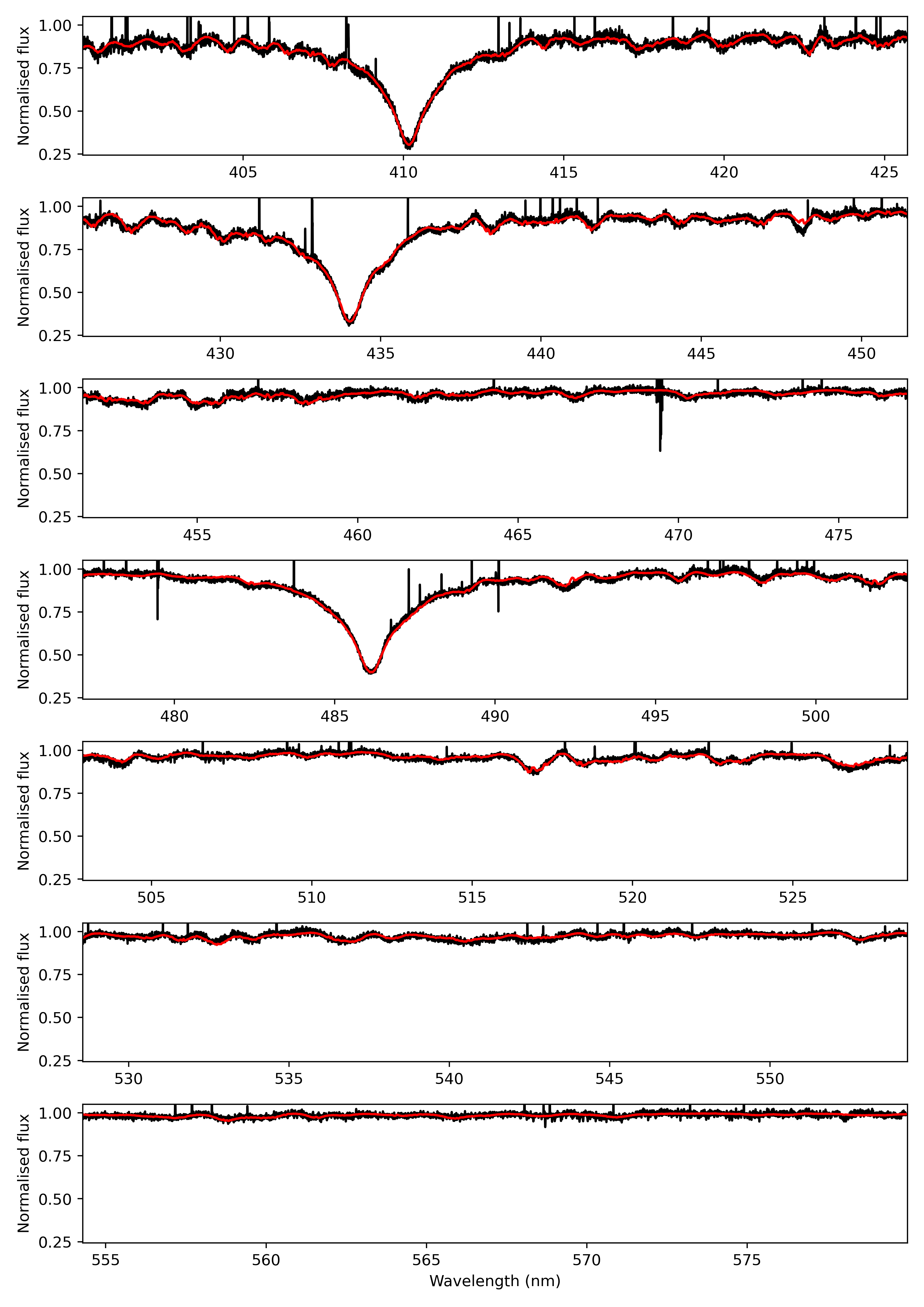
Figure 66: Spectrum of TIC 410452218 observed at 2023-03-16T02:37:05.256. The red line is the best-fitting theoretical spectrum.

References

- Abt (1979) Abt, H. A. 1979, ApJ, 230, 485
- Abt et al. (1969) Abt, H. A., Clements, A. E., Doose, L. R., & Harris, D. H. 1969, AJ, 74, 1153
- Abt & Levy (1972) Abt, H. A. & Levy, S. G. 1972, ApJ, 172, 355
- Aerts (2021) Aerts, C. 2021, Reviews of Modern Physics, 93, 015001
- Aerts et al. (2010) Aerts, C., Christensen-Dalsgaard, J., & Kurtz, D. W. 2010, Asteroseismology, Springer-Verlag, Heidelberg
- Aerts & De Cat (2003) Aerts, C. & De Cat, P. 2003, Space Sci. Rev., 105, 453
- Aerts & Mathis (2023) Aerts, C. & Mathis, S. 2023, A&A, 677, A68
- Aerts et al. (2019) Aerts, C., Mathis, S., & Rogers, T. M. 2019, ARA&A, 57, 35
- Aerts et al. (2023) Aerts, C., Molenberghs, G., & De Ridder, J. 2023, A&A, 672, A183
- Aerts et al. (2018) Aerts, C., Molenberghs, G., Michielsen, M., et al. 2018, ApJS, 237, 15
- Aerts et al. (2003) Aerts, C., Thoul, A., Daszyńska, J., et al. 2003, Science, 300, 1926
- Anderson et al. (1990) Anderson, E. R., Duvall, Thomas L., J., & Jefferies, S. M. 1990, ApJ, 364, 699
- Andrae et al. (2018) Andrae, R., Fouesneau, M., Creevey, O., et al. 2018, A&A, 616, A8
- Antoci et al. (2014) Antoci, V., Cunha, M., Houdek, G., et al. 2014, ApJ, 796, 118
- Antonello & Mantegazza (1986) Antonello, E. & Mantegazza, L. 1986, A&A, 164, 40
- Asplund et al. (2009) Asplund, M., Grevesse, N., Sauval, A. J., & Scott, P. 2009, ARA&A, 47, 481
- Astropy Collaboration et al. (2013) Astropy Collaboration, Robitaille, T. P., Tollerud, E. J., et al. 2013, A&A, 558, A33
- Bagnulo et al. (2003) Bagnulo, S., Landstreet, J. D., Lo Curto, G., Szeifert, T., & Wade, G. A. 2003, A&A, 403, 645
- Bailey et al. (2018) Bailey, J. I., Mateo, M., White, R. J., Shectman, S. A., & Crane, J. D. 2018, MNRAS, 475, 1609
- Balona & Dziembowski (2011) Balona, L. A. & Dziembowski, W. A. 2011, MNRAS, 417, 591
- Balona et al. (1994) Balona, L. A., Krisciunas, K., & Cousins, A. W. J. 1994, MNRAS, 270, 905
- Barceló Forteza et al. (2020) Barceló Forteza, S., Moya, A., Barrado, D., et al. 2020, A&A, 638, A59
- Barceló Forteza et al. (2018) Barceló Forteza, S., Roca Cortés, T., & García, R. A. 2018, A&A, 614, A46
- Barnes (2003) Barnes, S. A. 2003, ApJ, 586, 464
- Barnes (2007) Barnes, S. A. 2007, ApJ, 669, 1167
- Barrett et al. (2005) Barrett, P., Hunter, J., Miller, J. T., Hsu, J. C., & Greenfield, P. 2005, in Astronomical Society of the Pacific Conference Series, Vol. 347, Astronomical Data Analysis Software and Systems XIV, ed. P. Shopbell, M. Britton, & R. Ebert, 91
- Bastian & de Mink (2009) Bastian, N. & de Mink, S. E. 2009, MNRAS, 398, L11
- Bastian et al. (2018) Bastian, N., Kamann, S., Cabrera-Ziri, I., et al. 2018, MNRAS, 480, 3739
- Bastian et al. (2016) Bastian, N., Niederhofer, F., Kozhurina-Platais, V., et al. 2016, MNRAS, 460, L20
- Basu & Chaplin (2017) Basu, S. & Chaplin, W. J. 2017, Asteroseismic Data Analysis: Foundations and Techniques
- Basu et al. (2011) Basu, S., Grundahl, F., Stello, D., et al. 2011, ApJ, 729, L10
- Bedding et al. (2023) Bedding, T. R., Murphy, S. J., Crawford, C., et al. 2023, ApJ, 946, L10
- Bedding et al. (2020) Bedding, T. R., Murphy, S. J., Hey, D. R., et al. 2020, Nature, 581, 147
- Bertelli et al. (2003) Bertelli, G., Nasi, E., Girardi, L., et al. 2003, AJ, 125, 770
- Bouabid et al. (2013) Bouabid, M. P., Dupret, M. A., Salmon, S., et al. 2013, MNRAS, 429, 2500
- Bouchaud et al. (2020) Bouchaud, K., Domiciano de Souza, A., Rieutord, M., Reese, D. R., & Kervella, P. 2020, A&A, 633, A78
- Bouma et al. (2021) Bouma, L. G., Curtis, J. L., Hartman, J. D., Winn, J. N., & Bakos, G. Á. 2021, AJ, 162, 197
- Bowman & Kurtz (2018) Bowman, D. M. & Kurtz, D. W. 2018, MNRAS, 476, 3169
- Brahm et al. (2017) Brahm, R., Jordán, A., & Espinoza, N. 2017, PASP, 129, 034002
- Brandt & Huang (2015) Brandt, T. D. & Huang, C. X. 2015, ApJ, 807, 25
- Brasseur et al. (2019) Brasseur, C. E., Phillip, C., Fleming, S. W., Mullally, S. E., & White, R. L. 2019, Astrocut: Tools for creating cutouts of TESS images, Astrophysics Source Code Library, record ascl:1905.007
- Cantat-Gaudin et al. (2018) Cantat-Gaudin, T., Jordi, C., Vallenari, A., et al. 2018, A&A, 618, A93
- Casagrande & VandenBerg (2018) Casagrande, L. & VandenBerg, D. A. 2018, MNRAS, 479, L102
- Choi et al. (2016) Choi, J., Dotter, A., Conroy, C., et al. 2016, ApJ, 823, 102
- Christophe et al. (2018) Christophe, S., Ballot, J., Ouazzani, R. M., Antoci, V., & Salmon, S. J. A. J. 2018, A&A, 618, A47
- Corbard et al. (1999) Corbard, T., Blanc-Féraud, L., Berthomieu, G., & Provost, J. 1999, A&A, 344, 696
- Correnti et al. (2015) Correnti, M., Goudfrooij, P., Puzia, T. H., & de Mink, S. E. 2015, MNRAS, 450, 3054
- Cox (1955) Cox, A. N. 1955, ApJ, 121, 628
- Danielski et al. (2018) Danielski, C., Babusiaux, C., Ruiz-Dern, L., Sartoretti, P., & Arenou, F. 2018, A&A, 614, A19
- D’Antona et al. (2015) D’Antona, F., Di Criscienzo, M., Decressin, T., et al. 2015, MNRAS, 453, 2637
- De Cat & Aerts (2002) De Cat, P. & Aerts, C. 2002, A&A, 393, 965
- Deheuvels et al. (2015) Deheuvels, S., Ballot, J., Beck, P. G., et al. 2015, A&A, 580, A96
- Deheuvels et al. (2020) Deheuvels, S., Ballot, J., Eggenberger, P., et al. 2020, A&A, 641, A117
- Deheuvels et al. (2014) Deheuvels, S., Doğan, G., Goupil, M. J., et al. 2014, A&A, 564, A27
- Deubner et al. (1979) Deubner, F. L., Ulrich, R. K., & Rhodes, E. J., J. 1979, A&A, 72, 177
- Di Mauro et al. (2016) Di Mauro, M. P., Ventura, R., Cardini, D., et al. 2016, ApJ, 817, 65
- Domiciano de Souza et al. (2003) Domiciano de Souza, A., Kervella, P., Jankov, S., et al. 2003, A&A, 407, L47
- Dotter (2016) Dotter, A. 2016, ApJS, 222, 8
- Dupret et al. (2005) Dupret, M. A., Grigahcène, A., Garrido, R., Gabriel, M., & Scuflaire, R. 2005, A&A, 435, 927
- Eggen (1964) Eggen, O. J. 1964, in The Galaxy and the Magellanic Clouds, ed. F. J. Kerr, Vol. 20, 10
- Endal & Sofia (1978) Endal, A. S. & Sofia, S. 1978, ApJ, 220, 279
- Espinosa Lara & Rieutord (2011) Espinosa Lara, F. & Rieutord, M. 2011, A&A, 533, A43
- Feinstein et al. (1973) Feinstein, A., Marraco, H. G., & Mirabel, I. 1973, A&AS, 9, 233
- Foreman-Mackey (2016) Foreman-Mackey, D. 2016, The Journal of Open Source Software, 1, 24
- Foreman-Mackey et al. (2013) Foreman-Mackey, D., Hogg, D. W., Lang, D., & Goodman, J. 2013, PASP, 125, 306
- Frémat et al. (2023a) Frémat, Y., Royer, F., Marchal, O., et al. 2023a, A&A, 674, A8
- Frémat et al. (2023b) Frémat, Y., Royer, F., Marchal, O., et al. 2023b, A&A, 674, A8
- Fritzewski et al. (2020) Fritzewski, D. J., Barnes, S. A., James, D. J., & Strassmeier, K. G. 2020, A&A, 641, A51
- Fritzewski et al. (2023) Fritzewski, D. J., Van Reeth, T., Aerts, C., et al. 2023, A&A, in press, arXiv:2310.18426
- Gaia Collaboration et al. (2023a) Gaia Collaboration, De Ridder, J., Ripepi, V., & Aerts, C. 2023a, A&A, 674, A36
- Gaia Collaboration et al. (2023b) Gaia Collaboration, Vallenari, A., Brown, A. G. A., & Prusti, T. 2023b, A&A, 674, A1
- Garcia et al. (2022a) Garcia, S., Van Reeth, T., De Ridder, J., & Aerts, C. 2022a, A&A, 668, A137
- Garcia et al. (2022b) Garcia, S., Van Reeth, T., De Ridder, J., et al. 2022b, A&A, 662, A82
- Gebruers et al. (2022) Gebruers, S., Tkachenko, A., Bowman, D. M., et al. 2022, A&A, 665, A36
- Gehan et al. (2018) Gehan, C., Mosser, B., Michel, E., Samadi, R., & Kallinger, T. 2018, A&A, 616, A24
- Gieseking & Karimie (1982) Gieseking, F. & Karimie, M. T. 1982, A&AS, 49, 497
- Ginsburg et al. (2019) Ginsburg, A., Sipőcz, B. M., Brasseur, C. E., et al. 2019, AJ, 157, 98
- Girardi et al. (2013) Girardi, L., Goudfrooij, P., Kalirai, J. S., et al. 2013, MNRAS, 431, 3501
- Glatt et al. (2009) Glatt, K., Grebel, E. K., Gallagher, John S., I., et al. 2009, AJ, 138, 1403
- González & Lapasset (2000) González, J. F. & Lapasset, E. 2000, AJ, 119, 2296
- Goodman & Weare (2010) Goodman, J. & Weare, J. 2010, Communications in Applied Mathematics and Computational Science, 5, 65
- Gossage et al. (2019) Gossage, S., Conroy, C., Dotter, A., et al. 2019, ApJ, 887, 199
- Goupil et al. (2005) Goupil, M. J., Dupret, M. A., Samadi, R., et al. 2005, Journal of Astrophysics and Astronomy, 26, 249
- Granada et al. (2018) Granada, A., Jones, C. E., Sigut, T. A. A., et al. 2018, AJ, 155, 50
- Gratton et al. (2012) Gratton, R. G., Carretta, E., & Bragaglia, A. 2012, A&A Rev., 20, 50
- Handler (2009) Handler, G. 2009, in American Institute of Physics Conference Series, Vol. 1170, Stellar Pulsation: Challenges for Theory and Observation, ed. J. A. Guzik & P. A. Bradley, 403–409
- Harris et al. (2020) Harris, C. R., Millman, K. J., van der Walt, S. J., et al. 2020, Nature, 585, 357
- Hasanzadeh et al. (2021) Hasanzadeh, A., Safari, H., & Ghasemi, H. 2021, MNRAS, 505, 1476
- Healy & McCullough (2020) Healy, B. F. & McCullough, P. R. 2020, ApJ, 903, 99
- Hekker et al. (2011) Hekker, S., Basu, S., Stello, D., et al. 2011, A&A, 530, A100
- Henneco et al. (2021) Henneco, J., Van Reeth, T., Prat, V., et al. 2021, A&A, 648, A97
- Houdek (2000) Houdek, G. 2000, in Astronomical Society of the Pacific Conference Series, Vol. 210, Delta Scuti and Related Stars, ed. M. Breger & M. Montgomery, 454
- Huat et al. (2009) Huat, A. L., Hubert, A. M., Baudin, F., et al. 2009, A&A, 506, 95
- Jackiewicz (2021) Jackiewicz, J. 2021, Frontiers in Astronomy and Space Sciences, 7, 102
- Jian et al. (2023) Jian, M., Matsunaga, N., Jiang, B., Yuan, H., & Zhang, R. 2023, arXiv e-prints, arXiv:2311.08395
- Kaufer et al. (1999) Kaufer, A., Stahl, O., Tubbesing, S., et al. 1999, The Messenger, 95, 8
- Kaye et al. (1999) Kaye, A. B., Handler, G., Krisciunas, K., Poretti, E., & Zerbi, F. M. 1999, PASP, 111, 840
- Kippenhahn & Thomas (1970) Kippenhahn, R. & Thomas, H. C. 1970, in IAU Colloq. 4: Stellar Rotation, ed. A. Slettebak, 20
- Koester & Reimers (1996) Koester, D. & Reimers, D. 1996, A&A, 313, 810
- Kraft (1967) Kraft, R. P. 1967, ApJ, 150, 551
- Kurtz et al. (2023) Kurtz, D. W., Jayaraman, R., Sowicka, P., et al. 2023, MNRAS, 521, 4765
- Kurtz et al. (2014) Kurtz, D. W., Saio, H., Takata, M., et al. 2014, MNRAS, 444, 102
- Kurtz et al. (2015) Kurtz, D. W., Shibahashi, H., Murphy, S. J., Bedding, T. R., & Bowman, D. M. 2015, MNRAS, 450, 3015
- Ledoux (1951) Ledoux, P. 1951, ApJ, 114, 373
- Lee & Saio (1987) Lee, U. & Saio, H. 1987, MNRAS, 224, 513
- Lee & Saio (1997) Lee, U. & Saio, H. 1997, ApJ, 491, 839
- Li et al. (2016) Li, C., de Grijs, R., Deng, L., et al. 2016, Nature, 529, 502
- Li et al. (2019a) Li, C., Sun, W., de Grijs, R., et al. 2019a, ApJ, 876, 65
- Li et al. (2019b) Li, G., Bedding, T. R., Murphy, S. J., et al. 2019b, MNRAS, 482, 1757
- Li et al. (2019c) Li, G., Bedding, T. R., Murphy, S. J., et al. 2019c, MNRAS, 482, 1757
- Li et al. (2020a) Li, G., Guo, Z., Fuller, J., et al. 2020a, MNRAS, 497, 4363
- Li et al. (2019d) Li, G., Van Reeth, T., Bedding, T. R., Murphy, S. J., & Antoci, V. 2019d, MNRAS, 487, 782
- Li et al. (2020b) Li, G., Van Reeth, T., Bedding, T. R., et al. 2020b, MNRAS, 491, 3586
- Lightkurve Collaboration et al. (2018a) Lightkurve Collaboration, Cardoso, J. V. d. M., Hedges, C., et al. 2018a, Lightkurve: Kepler and TESS time series analysis in Python, Astrophysics Source Code Library, record ascl:1812.013
- Lightkurve Collaboration et al. (2018b) Lightkurve Collaboration, Cardoso, J. V. d. M., Hedges, C., et al. 2018b, Lightkurve: Kepler and TESS time series analysis in Python, Astrophysics Source Code Library, record ascl:1812.013
- Lim et al. (2019) Lim, B., Rauw, G., Nazé, Y., et al. 2019, Nature Astronomy, 3, 76
- Lomb (1976) Lomb, N. R. 1976, Ap&SS, 39, 447
- Lund et al. (2016) Lund, M. N., Basu, S., Silva Aguirre, V., et al. 2016, MNRAS, 463, 2600
- Maeder (2009) Maeder, A. 2009, Physics, Formation and Evolution of Rotating Stars, Springer-Verlag, Heidelberg
- Maitzen & Hensberge (1981) Maitzen, H. M. & Hensberge, H. 1981, A&A, 96, 151
- Martins & Palacios (2013) Martins, F. & Palacios, A. 2013, A&A, 560, A16
- Mathis (2009) Mathis, S. 2009, A&A, 506, 811
- Mathis (2013) Mathis, S. 2013, in Lecture Notes in Physics, Berlin Springer Verlag, ed. M. Goupil, K. Belkacem, C. Neiner, F. Lignières, & J. J. Green, Vol. 865, 23
- McAlister et al. (2005) McAlister, H. A., ten Brummelaar, T. A., Gies, D. R., et al. 2005, ApJ, 628, 439
- McQuillan et al. (2014) McQuillan, A., Mazeh, T., & Aigrain, S. 2014, ApJS, 211, 24
- Meilland et al. (2007) Meilland, A., Stee, P., Vannier, M., et al. 2007, A&A, 464, 59
- Meingast & Alves (2019) Meingast, S. & Alves, J. 2019, A&A, 621, L3
- Meingast et al. (2021) Meingast, S., Alves, J., & Rottensteiner, A. 2021, A&A, 645, A84
- Meynet et al. (1993) Meynet, G., Mermilliod, J. C., & Maeder, A. 1993, A&AS, 98, 477
- Michielsen et al. (2021) Michielsen, M., Aerts, C., & Bowman, D. M. 2021, A&A, 650, A175
- Moe & Di Stefano (2017) Moe, M. & Di Stefano, R. 2017, ApJS, 230, 15
- Mombarg (2023) Mombarg, J. S. G. 2023, A&A, 677, A63
- Mombarg et al. (2022) Mombarg, J. S. G., Dotter, A., Rieutord, M., et al. 2022, ApJ, 925, 154
- Mombarg et al. (2020) Mombarg, J. S. G., Dotter, A., Van Reeth, T., et al. 2020, ApJ, 895, 51
- Mombarg et al. (2023) Mombarg, J. S. G., Rieutord, M., & Espinosa Lara, F. 2023, A&A, 677, L5
- Mombarg et al. (2021) Mombarg, J. S. G., Van Reeth, T., & Aerts, C. 2021, A&A, 650, A58
- Mombarg et al. (2019) Mombarg, J. S. G., Van Reeth, T., Pedersen, M. G., et al. 2019, MNRAS, 485, 3248
- Montgomery & O’Donoghue (1999) Montgomery, M. H. & O’Donoghue, D. 1999, Delta Scuti Star Newsletter, 13, 28
- Mosser et al. (2012) Mosser, B., Goupil, M. J., Belkacem, K., et al. 2012, A&A, 548, A10
- Murphy et al. (2022) Murphy, S. J., Bedding, T. R., White, T. R., et al. 2022, MNRAS, 511, 5718
- Murphy et al. (2016) Murphy, S. J., Fossati, L., Bedding, T. R., et al. 2016, MNRAS, 459, 1201
- Murphy et al. (2019) Murphy, S. J., Hey, D., Van Reeth, T., & Bedding, T. R. 2019, MNRAS, 485, 2380
- Murphy et al. (2021) Murphy, S. J., Joyce, M., Bedding, T. R., White, T. R., & Kama, M. 2021, MNRAS, 502, 1633
- Murphy et al. (2020) Murphy, S. J., Saio, H., Takada-Hidai, M., et al. 2020, MNRAS, 498, 4272
- Neiner et al. (2020) Neiner, C., Lee, U., Mathis, S., et al. 2020, A&A, 644, A9
- Netzel et al. (2022) Netzel, H., Pietrukowicz, P., Soszyński, I., & Wrona, M. 2022, MNRAS, 510, 1748
- Ouazzani et al. (2020) Ouazzani, R. M., Lignières, F., Dupret, M. A., et al. 2020, A&A, 640, A49
- Ouazzani et al. (2019) Ouazzani, R. M., Marques, J. P., Goupil, M. J., et al. 2019, A&A, 626, A121
- Ouazzani et al. (2017) Ouazzani, R.-M., Salmon, S. J. A. J., Antoci, V., et al. 2017, MNRAS, 465, 2294
- Palakkatharappil & Creevey (2023) Palakkatharappil, D. B. & Creevey, O. L. 2023, A&A, 674, A146
- Pamos Ortega et al. (2023) Pamos Ortega, D., Mirouh, G. M., García Hernández, A., Suárez Yanes, J. C., & Barceló Forteza, S. 2023, A&A, 675, A167
- Pamyatnykh (1999) Pamyatnykh, A. A. 1999, Acta Astron., 49, 119
- pandas development team (2020) pandas development team, T. 2020, pandas-dev/pandas: Pandas
- Pápics et al. (2014) Pápics, P. I., Moravveji, E., Aerts, C., et al. 2014, A&A, 570, A8
- Paxton et al. (2011) Paxton, B., Bildsten, L., Dotter, A., et al. 2011, ApJS, 192, 3
- Paxton et al. (2013) Paxton, B., Cantiello, M., Arras, P., et al. 2013, ApJS, 208, 4
- Paxton et al. (2015) Paxton, B., Marchant, P., Schwab, J., et al. 2015, ApJS, 220, 15
- Paxton et al. (2018) Paxton, B., Schwab, J., Bauer, E. B., et al. 2018, ApJS, 234, 34
- Paxton et al. (2019) Paxton, B., Smolec, R., Schwab, J., et al. 2019, ApJS, 243, 10
- Pedersen et al. (2021) Pedersen, M. G., Aerts, C., Pápics, P. I., et al. 2021, Nature Astronomy, 5, 715
- Pedersen et al. (2018) Pedersen, M. G., Aerts, C., Pápics, P. I., & Rogers, T. M. 2018, A&A, 614, A128
- Pérez Hernández et al. (1999) Pérez Hernández, F., Claret, A., Hernández, M. M., & Michel, E. 1999, A&A, 346, 586
- Reed et al. (2000) Reed, M. D., Kilkenny, D., Kawaler, S. D., et al. 2000, Baltic Astronomy, 9, 183
- Reimers & Koester (1982) Reimers, D. & Koester, D. 1982, A&A, 116, 341
- Ricker et al. (2015) Ricker, G. R., Winn, J. N., Vanderspek, R., et al. 2015, Journal of Astronomical Telescopes, Instruments, and Systems, 1, 014003
- Riello et al. (2021) Riello, M., De Angeli, F., Evans, D. W., et al. 2021, A&A, 649, A3
- Ripepi et al. (2015) Ripepi, V., Balona, L., Catanzaro, G., et al. 2015, MNRAS, 454, 2606
- Royer et al. (2007) Royer, F., Zorec, J., & Gómez, A. E. 2007, A&A, 463, 671
- Saio et al. (2018) Saio, H., Bedding, T. R., Kurtz, D. W., et al. 2018, MNRAS, 477, 2183
- Saio et al. (2015) Saio, H., Kurtz, D. W., Takata, M., et al. 2015, MNRAS, 447, 3264
- Saio et al. (2021) Saio, H., Takata, M., Lee, U., Li, G., & Van Reeth, T. 2021, MNRAS, 502, 5856
- Sandquist et al. (2020) Sandquist, E. L., Stello, D., Arentoft, T., et al. 2020, AJ, 159, 96
- Scargle (1982) Scargle, J. D. 1982, ApJ, 263, 835
- Shajn & Struve (1929) Shajn, G. & Struve, O. 1929, MNRAS, 89, 222
- Shibahashi (1979) Shibahashi, H. 1979, PASJ, 31, 87
- Skumanich (1972) Skumanich, A. 1972, ApJ, 171, 565
- Stassun et al. (2019) Stassun, K. G., Oelkers, R. J., Paegert, M., et al. 2019, AJ, 158, 138
- Stellingwerf (1979) Stellingwerf, R. F. 1979, ApJ, 227, 935
- Stello et al. (2010) Stello, D., Basu, S., Bruntt, H., et al. 2010, ApJ, 713, L182
- Sterken (2005) Sterken, C. 2005, in Astronomical Society of the Pacific Conference Series, Vol. 335, The Light-Time Effect in Astrophysics: Causes and cures of the O-C diagram, ed. C. Sterken, 3
- Sterken & Jerzykiewicz (1993) Sterken, C. & Jerzykiewicz, M. 1993, Space Sci. Rev., 62, 95
- Straumit et al. (2022) Straumit, I., Tkachenko, A., Gebruers, S., et al. 2022, AJ, 163, 236
- Sung et al. (2002) Sung, H., Bessell, M. S., Lee, B.-W., & Lee, S.-G. 2002, AJ, 123, 290
- Szewczuk & Daszyńska-Daszkiewicz (2018) Szewczuk, W. & Daszyńska-Daszkiewicz, J. 2018, MNRAS, 478, 2243
- Tarricq et al. (2021) Tarricq, Y., Soubiran, C., Casamiquela, L., et al. 2021, A&A, 647, A19
- Terndrup et al. (2002) Terndrup, D. M., Pinsonneault, M., Jeffries, R. D., et al. 2002, ApJ, 576, 950
- Thompson et al. (1987) Thompson, I. B., Brown, D. N., & Landstreet, J. D. 1987, ApJS, 64, 219
- Tokuno & Takata (2022) Tokuno, T. & Takata, M. 2022, MNRAS, 514, 4140
- Townsend (2003) Townsend, R. H. D. 2003, MNRAS, 340, 1020
- Townsend et al. (2018) Townsend, R. H. D., Goldstein, J., & Zweibel, E. G. 2018, MNRAS, 475, 879
- Townsend & Teitler (2013) Townsend, R. H. D. & Teitler, S. A. 2013, MNRAS, 435, 3406
- Triana et al. (2017) Triana, S. A., Corsaro, E., De Ridder, J., et al. 2017, A&A, 602, A62
- Triana et al. (2015) Triana, S. A., Moravveji, E., Pápics, P. I., et al. 2015, ApJ, 810, 16
- Unno et al. (1989) Unno, W., Osaki, Y., Ando, H., Saio, H., & Shibahashi, H. 1989, Nonradial oscillations of stars
- Van Beeck et al. (2021) Van Beeck, J., Bowman, D. M., Pedersen, M. G., et al. 2021, A&A, 655, A59
- Van Reeth et al. (2016) Van Reeth, T., Tkachenko, A., & Aerts, C. 2016, A&A, 593, A120
- Van Reeth et al. (2015a) Van Reeth, T., Tkachenko, A., Aerts, C., et al. 2015a, A&A, 574, A17
- Van Reeth et al. (2015b) Van Reeth, T., Tkachenko, A., Aerts, C., et al. 2015b, A&A, 574, A17
- Van Reeth et al. (2015c) Van Reeth, T., Tkachenko, A., Aerts, C., et al. 2015c, ApJS, 218, 27
- von Zeipel (1924) von Zeipel, H. 1924, MNRAS, 84, 665
- Waelkens (1991) Waelkens, C. 1991, A&A, 246, 453
- Wang et al. (2022) Wang, C., Langer, N., Schootemeijer, A., et al. 2022, Nature Astronomy, 6, 480
- Winget et al. (1991) Winget, D. E., Nather, R. E., Clemens, J. C., et al. 1991, ApJ, 378, 326
- Wright et al. (2010) Wright, E. L., Eisenhardt, P. R. M., Mainzer, A. K., et al. 2010, AJ, 140, 1868
- Xiong et al. (2016) Xiong, D. R., Deng, L., Zhang, C., & Wang, K. 2016, MNRAS, 457, 3163
- Yu et al. (2018) Yu, J., Huber, D., Bedding, T. R., et al. 2018, ApJS, 236, 42
- Zahn et al. (2010) Zahn, J. P., Ranc, C., & Morel, P. 2010, A&A, 517, A7
- Zerbi et al. (1998) Zerbi, F. M., Mantegazza, L., Campana, S., & Antonello, E. 1998, PASP, 110, 804