Adding Corrections to Global Spherical Potentials for Use in a Coupled-Channel Formulation

Abstract

The coupled-channel technique augments a non-relativistic distorted wave born approximation scattering calculation to include a coupling to virtual states from the negative energy region. It has been found to be important in low energy nucleon-nucleus scattering. We modify the nucleon-nucleus standard optical potentials, not designed for a coupled-channel space, so they can be used in that setting. The changes are small and systematic. We use a standard scattering code to adjust a variety of optical potentials and targets such that the original fit to scattering observables are maintained as we incorporate the coupled-channel environment. Overall over forty target nuclei were tested from $A=12$ to $A=205$ and nucleon projectile energies from 1 MeV to 200 MeV. There is excellent improvement in fitting the scattering observables, especially for low energy neutron scattering. The corrections were found to be unimportant for projectile energies greater than 200 MeV. The largest changes are to the surface amplitudes while the real radii and the real central amplitude are modified by only a few percent, every other parameter is unchanged. This technique is general enough to be applied to a variety of inelastic theoretical calculations.

1 Introduction

The optical model nucleon-nucleus potential [1, 2] within a coupled-channel (CC) approach has a rich history (see an excellent review by Tamura [3]). The coupled-channel approach augments a non-relativistic Schrödinger approach by coupling the positive energy scattering problem with negative energy resonances, bound states, spectroscopic factors and transition potentials [4, 5]. A common issue is that the spherical distorted wave Born approximation (DWBA) optical potential is often phenomenologically fit lacking the coupled-channel context. The most widely used spherical global phenomenological optical model to date is from Koning and Delaroche [6] but there have been plenty of other similar attempts [7, 8, 9, 10, 11, 12, 13, 14, 15, 16, 17]. These models, being created in a DWBA context, are not directly suited for CC calculations especially at low energies [18]. There have been some attempts to fit the optical potential directly in a coupled-channel environment [19, 20, 21, 22]. There also has been work on adjusting the scattering (S) matrix of a single reaction DWBA optical potential to make it suitable for the coupled-channel calculation [23]. The present work takes another approach which is to augment the DWBA potential parameters in a global fashion by making slight modifications so that they are suitable for a coupled-channel methodology as other researchers have attempted in limited forms [24, 25, 18, 26, 27]. In the present work we expand these previous efforts by generalizing the corrections for the spherical DWBA to make these potentials appropriate for coupled-channel calculations. The improvements introduced are valid for a large range of projectile energies, target nuclei, and potentials.

To be clear, at low energy a spherical DWBA optical potential is not sufficient and other augmentations to the theory are needed including channel coupling, compound nucleus formation, and spectroscopic factors. However the researcher still needs functional optical potentials for the reactions and most often the spherical DWBA optical potential is the only available choice. If this spherical DWBA optical potential fits the elastic scattering data to a high degree and also has been fit to the total reaction experimental data and one wants these fits to be maintained than this prescription is a viable easy choice. A word on the importance of why the standard DWBA optical potentials must be changed before they are considered viable for CC calculations. The optical potential theory treats the target nucleus like a cloudy glass sphere where the elastic observables are treated directly (refracting from the sphere with no parameters) and the inelastic is described in only a gross fashion as the projectile beam that is absorbed by the cloudy sphere (with only the total inelastic cross-sections produced) and thus lost to other channels. Over the years methods using this optical potential have been devised to calculate specific inelastic reactions: excitation, breakup, exchange, fission, etc. These inelastic methods will include other parameters, transition potentials, or spectroscopic factors which are not included in the original optical potential. For the potential to remain consistent when the Hilbert space is changed to a non-spherical coupled channel we must maintain the integrity of the original refractive and absorptive properties. A good optical potential had these properties fit originally to experimental values (using elastic differential cross-sections, elastic spin experiments, and total reaction cross-sections) and thus it is essential that the integrity of these observables be maintained before any additional inelastic ingredients are included which require these equivalent gross properties for consistency.

2 Theoretical Frameworks

The phenomenological optical model potentials [6, 7, 28] used in this work contain the traditional volume ($V$), surface ($S$), and spin-orbit ($SO$) nuclear terms which are delineated using the standard Woods-Saxon form factors

$$f_{WS}(r,{\cal R}_{i},{\cal A}_{i})=(1+\exp\left((r-{\cal R}_{i})/{\cal A}_{i})\right)^{-1},$$ (1)

where ${\cal R}_{i}$ is the radius parameter and ${\cal A}_{i}$ is the diffusive parameter. The $i$ is a placeholder for the $V$, $S$, or $SO$ designation. The phenomenological optical model potentials takes a standard form:

$${\cal U}(r,E,A,N,Z)=$$

$$\Big{(}-{\cal V}_{V}(E,A,N,Z)-i{\cal W}_{V}(E,A,N,Z)\Big{)}f_{WS}(r,{\cal R}_{V},{\cal A}_{V})$$

$$+4{\cal A}_{S}\Big{(}{\cal V}_{D}(E,A)+i{\cal W}_{D}(E,A,N,Z)\Big{)}\frac{d}{dr}f_{WS}(r,{\cal R}_{D},{\cal A}_{D})$$

$$+\frac{2}{r}\Big{(}{\cal V}_{SO}(E,A,N,Z)+i{\cal W}_{SO}(E,A,N,Z)\Big{)}\frac{d}{dr}f_{WS}(r,{\cal R}_{SO},{\cal A}_{SO})({\bf l\cdot\sigma})$$

$$+f_{coul}(r,{\cal R}_{C},A,N,Z)$$ (2)

where the ${\cal V}_{i}$ and ${\cal W}_{i}$ are the real and imaginary potential amplitudes respectively and $f_{coul}(r,{\cal R}_{C},A,N,Z)$ is the coulomb term which has the following traditional format with a proton projectile:

$$f_{coul}(r,{\cal R}_{C},A,N,Z)=\frac{Ze^{2}}{r},\;\;\;\;\;r\geq{\cal R}_{C},$$

$$f_{coul}(r,{\cal R}_{C},A,N,Z)=\frac{Ze^{2}}{2{\cal R}_{C}}\Big{(}3-\frac{r^{2}}{{{\cal R}_{C}}^{2}}\Big{)},r\leq{\cal R}_{C}.$$ (3)

For a neutron projectile this term is set to zero. There were two optical potentials used in this work. Mainly we used the aforementioned Koning and Delaroche [6] which covers a large range of energies and targets. For targets below an atomic number (A) of 27 we used the potential of one of the authors [7, 28]. We believe that using two different potentials has increased the robustness of this technique.

In earlier research optical potentials have been modified so that they function in a coupled-channel (CC) approach so we give a brief overview of these past efforts. The TALYS scattering code [29, 25], which has as its direct scattering tool Raynal’s ECIS [4, 30, 31], state in the manual (all versions up through the present) that if a CC calculation is attempted and no potential is given then TALYS will use the DWBA potential KD03 [6] (our choice for $A>26$) but will reduce the imaginary surface term by 15% (which is denoted as ${\cal W}_{D}(E,A)$ in Eq. 2 of this work). Later Nobre et. al [18] used a suggestion by Bang and Vaagen [24] who were interested in studying the effects of deformation in nuclear orbitals. To conserve volume they modified the radius terms of the central potential, denoted above as ${\cal R}_{V}$ (volume) and ${\cal R}_{D}$ (surface)

$${{\cal R^{\prime}}_{i=V,D}}={{\cal R}_{i}}\big{(}1-\frac{{\sum_{\lambda}}\beta_{\lambda}^{2}}{4\pi}\big{)},$$ (4)

where $\beta_{\lambda}$ are the deformation parameters which make the nucleus non-spherical:

$${\cal R}^{\prime}_{i}(\theta,\phi)=R_{i}(1+\sum_{\lambda}\beta_{\lambda}Y^{0}_{\lambda}).$$ (5)

These researchers, using the modification prescribed in Eq. 4, found satisfactory results for neutron scattering off the rare-earth nuclei. Al-Rawashdeh and Jaghoub continued this investigation with the same modification to the actinide nuclei (A=227-250) and came to similar conclusions [26].

The corrections mentioned were relatively small [25, 18, 26]. For the present research we started with these same previous modifications: we lower the imaginary surface term, we also adjust the radius for the real volume, surface and additionally the spin-orbit terms as prescribed. Instead of a static 15% drop of the imaginary surface term we fit the imaginary and real surface terms to the original elastic and total reaction observables. We also slightly adjusted the depth of the real part of the central amplitude in an analytical fashion. This entire process was done for a large range of mass numbers (A=12-205) for the target and energies (1 MeV-205 MeV) for either the neutron and proton projectile. Many of the optical potential parameters were not adjusted hoping that this retains the original flavor of the DWBA potential (all diffusive parameters, ${\cal A_{i}}$, all imaginary radii, Im ${\cal R_{i}}$, the spin-orbit amplitude parameters $({\cal V}_{SO},{\cal W}_{SO})$, and the coulomb parameter (${\cal R}_{C}$) were untouched).

The most complicated aspect of this alteration was the modification of the surface which we believe is the aspect of the nucleus most changed by the distortion. Many researches have studied the importance of the surface term, and its corresponding surface energy, in nuclear reactions [32, 33, 34, 35, 36, 37]. The skin thickness of the nuclear matter plays a large roll in mimicking a distortion effect important in a coupled-channel calculation. Finding a standard prescription for the surface term was a struggle, the end result was to rely only on the observables and treat each set of reactions (fixed energy of projectile and target nucleus) as an independent entity thus fitting each surface amplitude to the entire set of results (cross-sections and spin observables). We had these realistic constraints:
$\bullet$ All elastic measurements and all total reaction cross-sections should be as closely preserved as possible to the original potential when it is used in a coupled-channel environment.
$\bullet$ As $\frac{{\sum_{\lambda}}\beta_{\lambda}^{2}}{4\pi}\to 0$ then the distortion effect should also head to zero.
$\bullet$ As the target size, $A$, approaches 200 the distortion dependence on $A$ should saturate
$\bullet$ If the projectile energy of the nucleon is near zero the distortion effect should be at a maximum.
$\bullet$ As the projectile energy of the nucleon increases the distortion effect should diminish towards zero.
$\bullet$ The surface terms should be modified with the ansatz: the smaller the change the better.
Although fitting the surface term is not analytical it provides the flexability needed for adjustments made to the theoretical system (number of channels and strength of each channel).

The total cross-sections deserve special mention in the thought process of our developed theory since they represent an interplay between the strength of the real and imaginary scattering amplitudes of the solution to the DWBA scattering problem. Since Eq. 4 reduces the radius this will affect the strength (the volume) of the reaction. This equation, as derived by Bang and Vaagen, was the first order term in an expansion to conserve the volume of the central term of the Woods-Saxon 1 during distortion. We agree that the volume should not change by much but the true measure of the quality of a modification (ie keep the strength of the potential the same) is to maintain the results of the proton-nucleus reaction cross-section and the neutron-nucleus reaction and total cross-section. The analytical function which approximates the solution to the volume integral of the Woods-Saxon, given in Ref. [6], as

$${\cal J}_{V} =\int_{allspace}(1+\exp\left((r-{\cal R}_{V})/{\cal A}_{V})\right)^{-1}\>d^{3}{\vec{r}}$$ (6)

$$=\frac{4}{3}\pi{\cal R}_{V}^{3}(1+(\frac{{\pi\cal A}_{V}}{{\cal R}_{V}})^{2})$$

is illustrative. We found, in the spirit of the phenomenological approach, that what worked best in maintaining the total cross-section observables was to adjust the real central amplitude by a prescription that uses the above equation. We found that the spherical volume was nearly conserved as was the magnitude of the surface term but ultimately our test was the measurable quantities (emphasizing not fitting to experimental results but instead fitting the distorted CC theoretical calculation to the original DWBA non-CC theoretical calculation). Our principle measure was therefore a weighted $\chi^{2}$ where we solely compared the difference in calculated theoretical observables. We also deemed the manner of the weighting of this $\chi^{2}$ to be important. The most important observables were the total neutron cross-sections, total reaction cross-sections, and the forward angles of the differential cross-section (with a regressive sliding scale as the angle increases). Of lesser importance were the backward angles of the differential cross-section, and the forward angles of the spin polarization, and of least importance were the backward angles of the polarization. For example the percent error for the differential cross-section standard deviation at 20, 90, and 160 degrees was 5%, 18%, and 31% respectively. Note that since most quality optical potentials are fit to a plethora of experimental data we felt that experiment was not being ignored, ultimately maintaining the quality of the original optical potential fit to the experimental elastic data and total inelastic data was the objective.

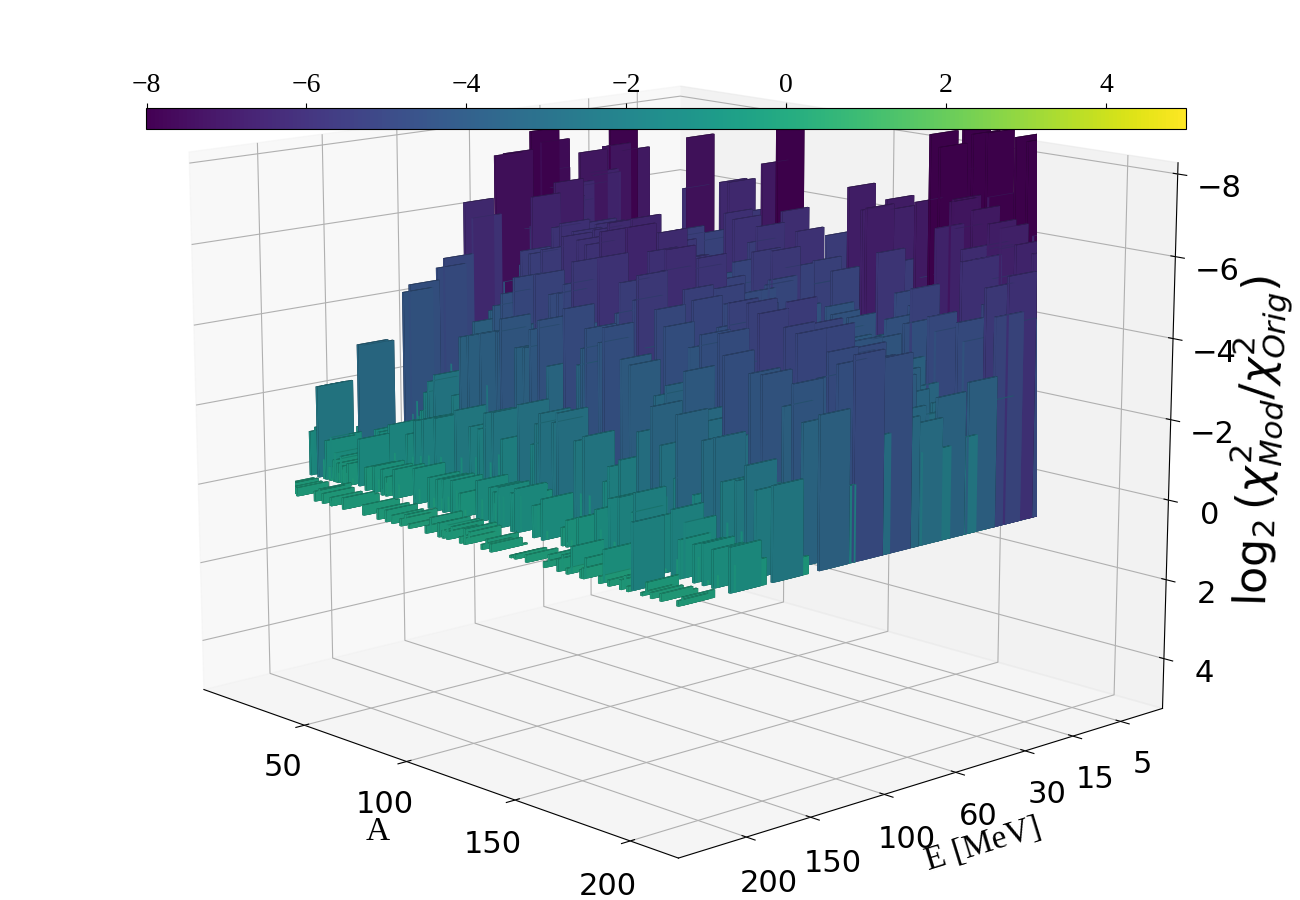
Figure 1: This shows the improvement on all of our results as a function of atomic number (A) and projectile energy (E). The amplitude is a ratio of the $\chi^{2}$ on the scattering observables for our modified coupled channel potential and the original optical potential both used in a coupled-channel environment. Note that this is on a $\log_{2}$ scale so a -8 refers to a reduction of a factor of 256 in the the $\chi^{2}$, more discussion is in the text.

Here follows a mathematical summary of our analytical changes which have been discussed in this section. First some definitions:

$${{\cal R}_{i}}^{\prime} = (1-\Delta_{R}){\cal R}_{i}$$

$$\Delta_{R} = \frac{60^{4}}{(E^{2}+60^{2})^{2}}\frac{{\sum_{\lambda}}\beta_{\lambda}^{2}}{4\pi}$$

$$\frac{{\cal J}_{V}}{{{\cal J}_{V}}^{\prime}} = (\frac{{\cal R}_{V}}{{{\cal R}_{V}}^{\prime}})^{3}\frac{1+(\pi a_{V}/{\cal R}_{V})^{2}}{1+(\pi a_{V}/{{\cal R}_{V}}^{\prime})^{2}}.$$ (7)

The volume integrals are ${{\cal J}_{V}}$, and we use the approximate analytical version found in Ref. [6]. The radius is changed by a $\Delta_{R}$ but there is a sliding energy scale attached to it, $\frac{60^{4}}{(E^{2}+60^{2})^{2}}$, this was not in earlier work [18, 26] which had as a focus low energy scattering. We found that the strongest dependence exhibited by coupled-channel calculations is projectile energy. At over 200 MeV the coupled-channel is nearly insignificant (see the next section for discussion) so we fitted an energy scale to our modifications. Now we list the four analytical changes:

$$Re({{\cal R}_{V}}^{\prime}) = (1-\Delta_{R})Re({{\cal R}_{V}})$$

$$Re({{\cal R}_{D}}^{\prime}) = (1-\Delta_{R})Re({{\cal R}_{D}})$$

$$Re({{\cal R}_{SO}}^{\prime}) = (1-\Delta_{R})Re({{\cal R}_{SO}})$$

$${{\cal V}_{V}}^{\prime} = (1-\Delta_{R})^{3}\frac{{\cal J}_{V}}{{{\cal J}_{V}}^{\prime}}{{\cal V}_{V}}_{0}$$ (8)

$$= \frac{1+(\pi a_{V}/{\cal R}_{V})^{2}}{1+(\pi a_{V}/{{\cal R}_{V}}^{\prime})^{2}}{{\cal V}_{V}}_{0}.$$

Lastly the optical potential fitted the real and imaginary surface amplitudes directly to the observables, most modern codes have this capability (TALYS [29, 25], FRESCO [38, 5], ECIS [4, 30, 31], and EMPIRE [39]). At most the surface amplitudes were changed by 6 MeV (upward for the real and downward for the imaginary). In summary a total of six parameters were changed to make these potentials CC ready. The surface terms were left adjustable because the coupling varies depending on the reaction or the theoretical model used. This prescription dictates a fixed change to the real radii, the real central amplitude, and the real spin-orbit amplitude but the reaction-model dependent fit is based on fitting the surface amplitudes correctly.

3 Results and Discussion

a

3.1 General Results

Energy	p/n	$\chi^{2}_{0}$	$\chi^{2}_{f}$
[MeV]
1.0	n	$2.1\times 10^{4}$	$1.5\times 10^{2}$
	p	$0.0$	$0.0$
5.0	n	$4.2\times 10^{3}$	$1.3\times 10^{2}$
	p	$7.3\times 10^{1}$	$1.1\times 10^{0}$
10.0	n	$1.7\times 10^{3}$	$5.6\times 10^{1}$
	p	$5.9\times 10^{2}$	$2.3\times 10^{1}$
20.0	n	$8.7\times 10^{2}$	$6.4\times 10^{1}$
	p	$1.7\times 10^{2}$	$2.0\times 10^{1}$
35.0	n	$9.3\times 10^{2}$	$5.1\times 10^{1}$
	p	$4.7\times 10^{2}$	$5.6\times 10^{1}$
65.0	n	$6.3\times 10^{2}$	$2.7\times 10^{1}$
	p	$4.1\times 10^{2}$	$3.4\times 10^{1}$
100.0	n	$2.0\times 10^{2}$	$3.0\times 10^{1}$
	p	$2.5\times 10^{2}$	$4.3\times 10^{1}$
130.0	n	$1.0\times 10^{2}$	$2.8\times 10^{1}$
	p	$7.6\times 10^{1}$	$4.0\times 10^{1}$
200.0	n	$4.5\times 10^{1}$	$4.0\times 10^{1}$
	p	$4.4\times 10^{1}$	$3.6\times 10^{1}$

Table 1: This summarizes our results at nine different projectile energies separated by the isospin of the projectile (p/n). The observables are a weighted chi squared which involved fitting to the differential cross-section, the differential polarization, the total reaction cross-section, and in the neutron projectile case the total cross-section. The initial chi squared ($\chi^{2}_{0}$) is the average $\chi^{2}$ difference between the unmodified optical potential in the couple channel calculation and the calculation not including coupled-channels. The final chi-squared ($\chi^{2}_{f}$) is nearly the same calculation - except we have added the improvements to the optical potential when using the coupled-channel. These are statistical averages but each value is the average of at least 25 points, for more analysis see the text.

Using the weighted $\chi^{2}$ ratio as our test, we tested over 40 nuclei at over 10 different energies and two projectiles (the proton and the neutron), thus over 1000 cases. Each case computed the differential cross-section, the polarization, the total reaction cross-section, and for a neutron projectile the total cross-section. Each case was run as a normal DWBA (using ECIS), then we ran it again (the same unmodified optical potential) in a coupled channel framework (again using ECIS). In this instance the potential was used incorrectly; a global spherical optical potential used in a coupled channel space. The purpose was as the control to see how much the couple-channel space distorted the original observable results. Finally it was run with our adjustments in this coupled-channel methodology to ascertain if we could bring the calculated quantities back to their original values.

The results of our modifications were very good, our weighted $\chi^{2}$ improvement ratio averaged 16 which our worst case was 1.25 (at high energy) and our best case was 400 (see Fig. 1). That is the weighted $\chi^{2}$ was reduced, on average, by a factor of 16. Figure 1 shows that the best improvement happened systematically at low energies, where the influence of coupled channels is the greatest. The smallest improvement happened at high energies, where the coupled channel effect is the least influential. This was our motivation for Eq. 7 where the projectile energy scale factor $\frac{60^{4}}{(E^{2}+60^{2})^{2}}$ quickly suppresses any changes such that at a projectile energy of 240 MeV the suppression factor for this modification (from a 0 MeV baseline) is about 300. The need for an energy scale is shown even more directly in the results of Table 1, which is a good summary of the benefits of the corrections. The $\chi^{2}$ drops after the improvements have been employed, especially with the neutron projectile observables at low energy. As the energy of the neutron projectile increases the changes become less and less important. The proton projectile does not follow these trends at low energies because the coulomb force dominates. There were calculation error-bars given to each calculated quantity such that the error at forward angles was larger than backward angles and the weighting of a total cross-section point was worth about one third of a complete differential data set (measured from 5^o to 174^o at low energies). If one was to convert the results of Table 1 to a reduced $\chi^{2}$, a $\chi^{2}$ of about 30 would be equivalent to a reduced $\chi^{2}$ of 1 in that every theoretical calculation point is within the error bars chosen by the researchers which were meant to imitate typical experimental errors, so good results indeed as many of the results of Table 1 approach 30. For example a projectile energy of 35 MeV has very typical results, if one follows the results at only 35 MeV in the figures below (Figs. 2-16) one will see good improvement in every observable. We also believe that the quality of the improvements will work when the neutron projectile energy is less than 1 MeV because the energy dependence at extreme low energies is near constant and the imaginary surface term, which should be small is reduced even smaller. Again all target nuclei at all projectile energies up to 200 MeV benefitted from these adjustments as Fig. 1 depicts. Without the alterations employed it can be seen that the $\chi^{2}$ is less than 50 for projectile energies of 200 MeV.

A word about the coupled-channel framework which is already familiar to many [40, 30, 41]. If the nucleus is non-spherical and has multi-pole deformations that are either causing an excited rotation and / or vibrational collective mode then we can calculate these collective excited observables. It starts by expanding the radius assuming a series of deformations

$$R(\theta)=R_{0}\left[1+\beta_{2}Y_{2}^{0}(\theta)+\beta_{4}Y_{4}^{0}(\theta)+\beta_{6}2Y_{6}^{0}(\theta)+\ldots\right],$$ (9)

where the $\beta_{\lambda}$’s are deformation parameters. In a rotational model these are corresponding to an quadrapole, hexapole, octupole rotational mode, where by symmetry, only even modes are allowed [42, 30]. There is a partial wave dependent asymmetry in the polar angle separating $\vec{r}$ and $\vec{r^{\prime}}$ in coordinate space. The same common multi-pole expansion can be performed on the optical potential, with $x=\cos(\theta)$

$$U_{\lambda}(|\vec{r}|,|\vec{r^{\prime}}|)=\frac{1}{2}\int_{-1}^{+1}U(\vec{r},\vec{r^{\prime},x}P_{\lambda}(x)\;dx.$$ (10)

where $R=\vec{r^{\prime}}-\vec{r}$. The vibrational mode looks similar:

$$R(\theta)=R_{0}\left[1+\sum_{\lambda}\alpha_{\lambda}\right],$$ (11)

where

$$\alpha_{\lambda}^{\mu}=\frac{\beta_{\lambda}^{\mu}}{\sqrt{2\lambda+1}}\left\{(b_{\lambda,\mu}+(-1)^{\mu}b^{+}_{\lambda,-\mu}\right\},$$ (12)

the $\mu$ stands for the magnetic quantum number and can be summed over to produce $\alpha_{\lambda}$. As can be seen the $\alpha_{\lambda}$ contain deformation parameters ($\beta_{\lambda}$), important for this work, and photon creation($b^{+}_{\lambda,-\mu}$) and destruction ($b_{\lambda,\mu}$) operators. With a vibrational mode the phonons can follow all allowed electric and magnetic transitions. One can then expand the potential in a Taylor series to first order as:

$$U(r,R)=U(r,R_{0})+\frac{d}{dR_{0}}U(r,R_{0})R_{0}\sum_{\lambda}\alpha_{\lambda}Y_{\lambda}(\theta,\phi).$$ (13)

So these phonon excitations are derived from the non-spherical nature of the nucleus. The vibrational, rotation, and a combination of both models can be calculated by common distorted born approximation codes [31, 38]. These codes take as input a optical potential and then place it into the chosen vibrational/rotational mode.

We assumed that each nuclei was either distorted using either a simple first-order vibrational or rotational model. We stuck to a convention that if $A<130$ it was vibrational, otherwise rotational (we loosen these restrictions later) with the caveat that if it was an even-odd or odd-even nucleus we always used vibrational because we had difficulty in getting ECIS to produce results otherwise (see Ref. [43] for a similar issue with ECIS studying even-odd Calcium isotopes). For each target we chose the deformation parameters, $\beta_{\lambda}$ from a variety of sources. We tried to rely on research that stemmed from an inelastic experiment but in their absence we used deformation parameters created from a theoretical framework, especially Ref. [44]. By using a plethora of sources for the distortion parameters we hope that the algorithm is robust. Once the initial research was finished we randomized the deformation parameter values in both directions multiple times, up to 30%, to see if the quality of the fits changed; they did not – the statistical analysis always produced similar improvements. In general, as opined earlier, the larger the deformation, the larger the modification, but besides that dependence the algorithm was stable. We used a deformed coulomb potential (with the same deformation parameter as every other term). When the potential was effectively only a coulomb force (when the proton could not penetrate the coulomb barrier at 1 MeV and at 5 MeV for large targets, see Table 1) the adjustments did very little which infers, as expected, that the long range coulomb was not sensitive to this research. For each nucleus we made it a point to include at least three excited states or coupled channels. In a later section we will study two nuclei where we will change the theoretical model and the reactions which are coupled to study the effect of this prescription on these variances.

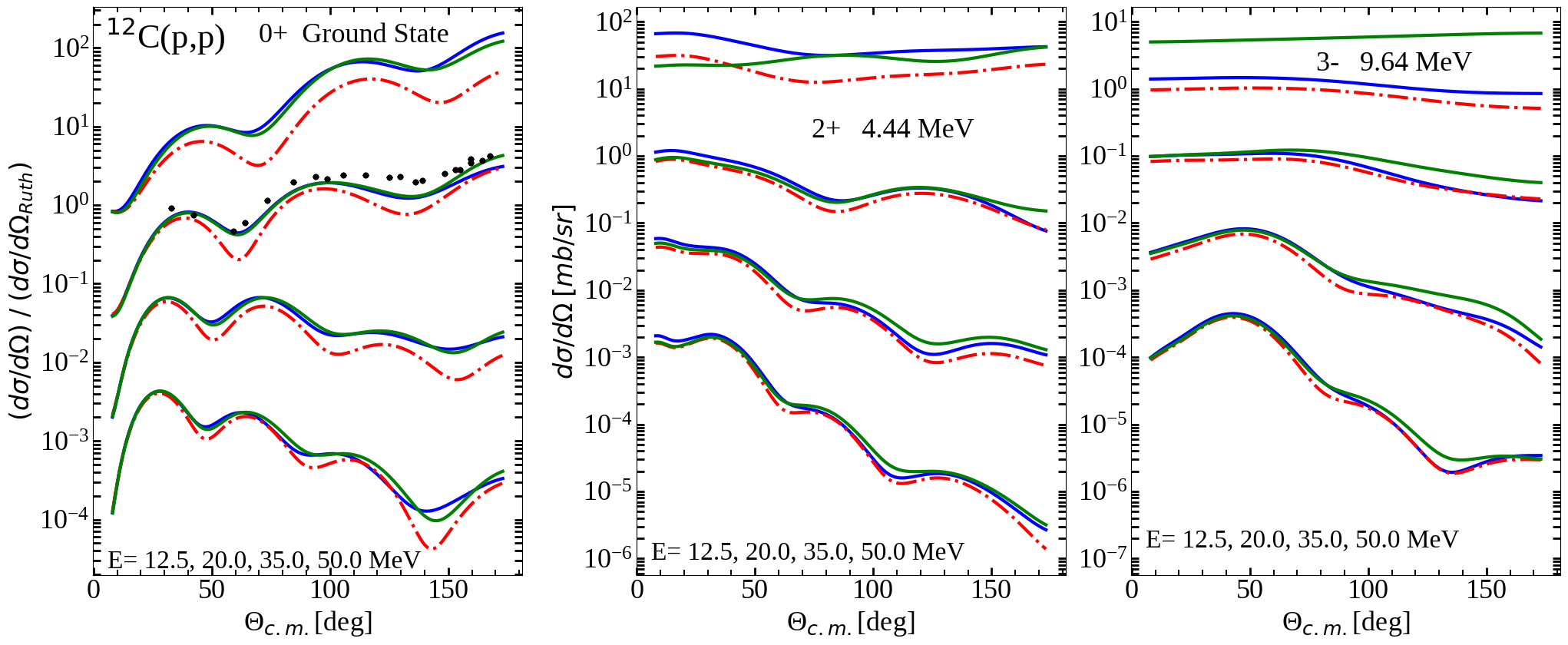
Figure 2: Differential cross-sections for a proton on ¹²C. In all calculations the solid blue line is a calculation using the original spherical DWBA potential, the solid green line has modified that potential and uses a coupled-channel calculation. The red dashed line is the inconsistent hybrid of the original potential used in a coupled-channel environment. The left panel represents the elastic (ground state only) differential cross-section divided by the Rutherford cross-Section for four different proton energies, lowest energy at the top, highest energy at the bottom. This left panel presents one of the observables which we fit to, a good fit would be when the solid green calculation is close to the original solid blue calculation. The central and right panel represent inelastic differential cross-sections which were not used in the fittings, they however show the sensitivity of the modification to the collective 2+ and 3- or 4+ inelastic cross-sections, again the projectile energies are the lowest at the top and highest at the bottom. For more analysis see the text. For aesthetics the E=20.0 MeV cross-sections have been reduced by a factor of 20, the E= 35.0 MeV by a factor of 400, the E = 50.0 by a factor of 8000. The experimental data at E = 20.0 MeV is from Ref. [45]. For ¹²C $\beta_{2}=-0.71$, $\beta_{3}=0.42$.

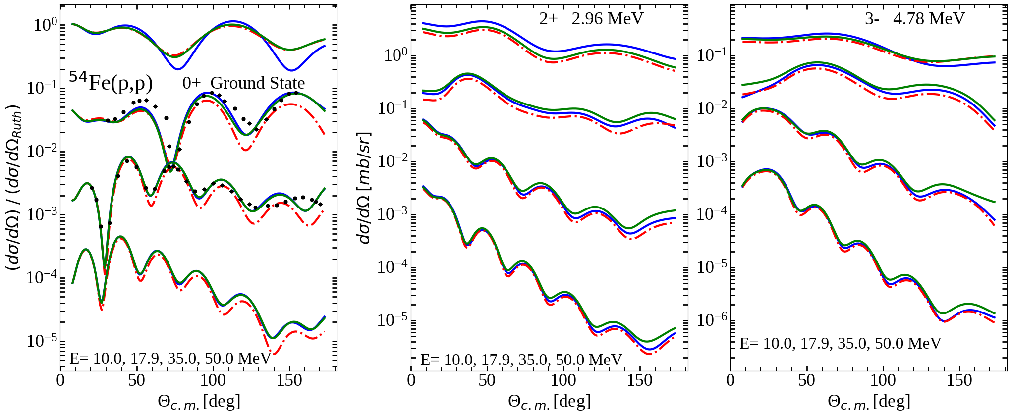
Figure 3: Differential cross-sections for a proton on ⁵⁴Fe. The legend and description is the same as Fig. 2. Note that the theoretical modification is poor at 10 MeV projectile energy, perhaps because the short term coulomb is important and it has not been modified, for more analysis see the text. For aesthetics the E=17.9 MeV cross-sections have been reduced by a factor of 20, the E= 35.0 MeV by a factor of 400, the E = 50.0 by a factor of 8000. The experimental data at E = 17.9 MeV is from Ref. [46], the experimental data from 35.0 MeV is from Ref. [47, 48] For ⁵⁴Fe $\beta_{2}=0.24$, $\beta_{3}=0.16$.

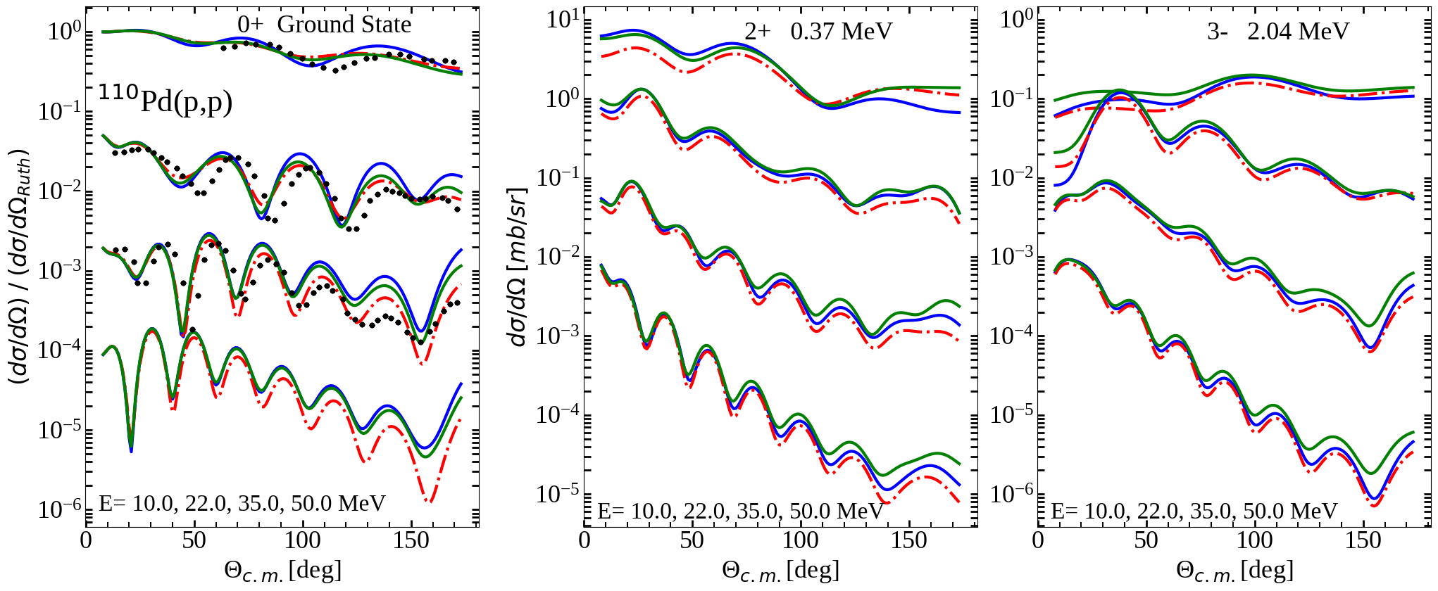
Figure 4: Differential cross-sections for a proton on ¹¹⁰Pd. The legend and description is the same as Fig. 2. Note that the theoretical modification is poor at 10 MeV projectile energy, perhaps because the short term coulomb is important and it has not been modified, for more analysis see the text. For aesthetics the E=22.0 MeV cross-sections have been reduced by a factor of 20, the E= 35.0 MeV by a factor of 400, the E = 50.0 by a factor of 8000. The experimental data at E = 22 MeV and 35 MeV is from Ref. [49]. For ¹¹⁰Pd $\beta_{2}=0.24$, $\beta_{3}=0.11$

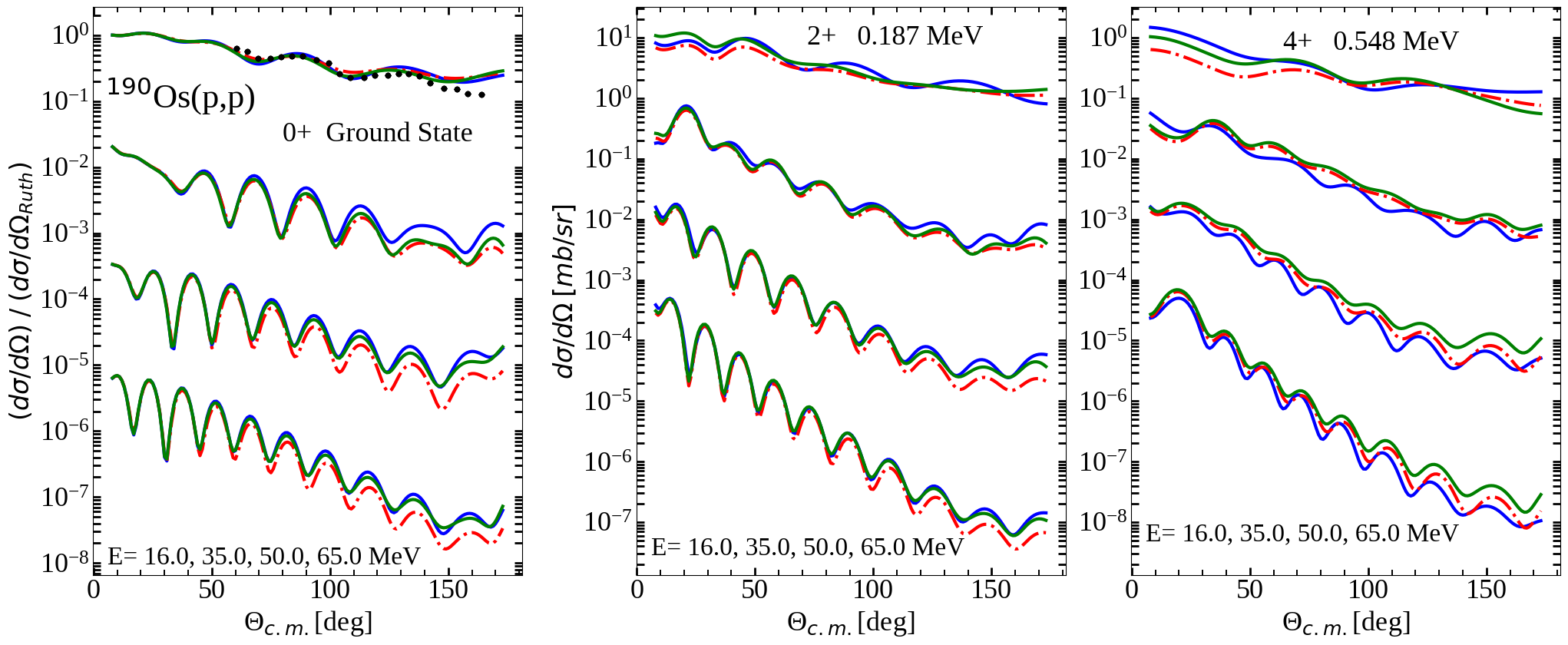
Figure 5: Differential cross-sections for a proton on ¹⁹⁰Os. The legend and description is the same as Fig. 2, for more analysis see the text. For aesthetics the E=35.0 MeV cross-sections have been reduced by a factor of 50, the E= 50.0 MeV by a factor of 2500, the E = 65.0 by a factor of 125000. The experimental data at E = 16 MeV is from Ref. [50].For ¹⁹⁰Os $\beta_{2}=.187$, $\beta_{4}=-.086$

As stated we had over a thousand cases, which meant over three-thousand different observables were tested. Since each case was independent, the fit was done in parallel, and the fitting procedure was done within the  it ECIS software which was the workhorse of this research. After getting a best fit for the real and imaginary surface terms from the code was run again with those parameters as input and the fitting process was done again. This step was repeated, usually 5-7 times, until convergence was reached. Overall the results were very consistent, the real surface term was increased from 0-6 MeV and the imaginary surface term was decreased by 0-6 MeV. To summarize, (1) the real central volume term was decreased in an analytical procedure, (2) the real central, surface, and spin-orbit radii were decreased in an analytical procedure (3) The real and imaginary surface amplitudes were lastly fit using ECIS.

We chose four nuclei for most of our representations in this work: ¹²C,⁵⁴Fe, ¹¹⁰Pd (all treated as a vibrator), and ¹⁹⁰Os (treated as a rotator), a small subset but representative of the data as a whole. All results with ${}^{12}C$ used the potential from Ref. [7], the rest used the optical potential of Ref. [6]. A good result for our solid green line modification is when it coincides often with the original solid blue line calculation on the left-most elastic observables graph only. The reason for the singling out of the first panel is that the optical potentials were fit only to the elastic scattering observables of the left panel. The two right panels represent usually the two lowest excited energy levels of the target nucleon. They are an integral part of our discussion but they were not used as part of the fitting routine.

Some systematic results that can be gleaned from these eight figures of differential cross-sections(2-9). As already discussed, at low energies the effects are more pronounced, thus here we displayed nothing over an energy of 65 MeV even though we calculated observables up to 200 MeV. Generally, our modification to the potentials returns the optical potential to close to its original status (green line coincides often with blue line in the leftmost panel), the largest effects and the largest $\chi^{2}$ happens at low projectile energy. The right two panels of each figure deserve mention. These represent the fit to the 2+ and 3- states. As stated earlier they were not used in developing the altercations however systematically what it shows in the differential cross-sections is that there is a distinct difference in the sensitivities of the deformation parameter between a coupled-channel calculation and a non coupled-channel calculation. Generally there have been large uncertainties on this deformation parameter (as an ${}^{16}O$ example see Ref. [51]) and generally strict theoretical calculations of this deformation parameter under predict their experimental counterparts (compare the ${}^{16}O$ experimental Ref. [51] to the theoretical Ref. [44]). Our results also show that there is an increased sensitivity to the parameter if our modified coupled-channel is used. Our corrected green solid line in the two rightmost panels of the differential cross-sections is often the calculation with the largest magnitude, (Figs. 2-9) thus showing a heightened influence of the deformation parameter ($\beta_{i}$); a smaller deformation value is needed to achieve fitting experimental observables. This coincides with the coupled channel calculation of Ref. [51] and it was also found by authors involved in this research ( Ranga et. al. submitted to Journal of Physics G).

Proton scattering at low energies is denominated by the coulomb force and thus our prescription has little effect at projectile energies which are approximately equivalent to or less than the couomb barrier. Since we do not adjust the coulomb parameter this is expected. It is also important to note that all these calculation except for carbon use Koning and Delaroche [6] global optical potential and sometimes the original fit is good (as for ${}^{5}4$Fe) and at other times the quality is less than desired (as for ${}^{1}10$Pd). This prescription was built to duplicate the original theoretical results so its validity is strongly correlatesd to the quality of the original fit. Carbon calculations used Refs. [7, 28] and the same statement is true. The fits for ¹²C varied and thus it is important to ascertain the quality of your original global potential before applying this prescription. This will become even more apparent with a neutron projectile (see Fig. 6).

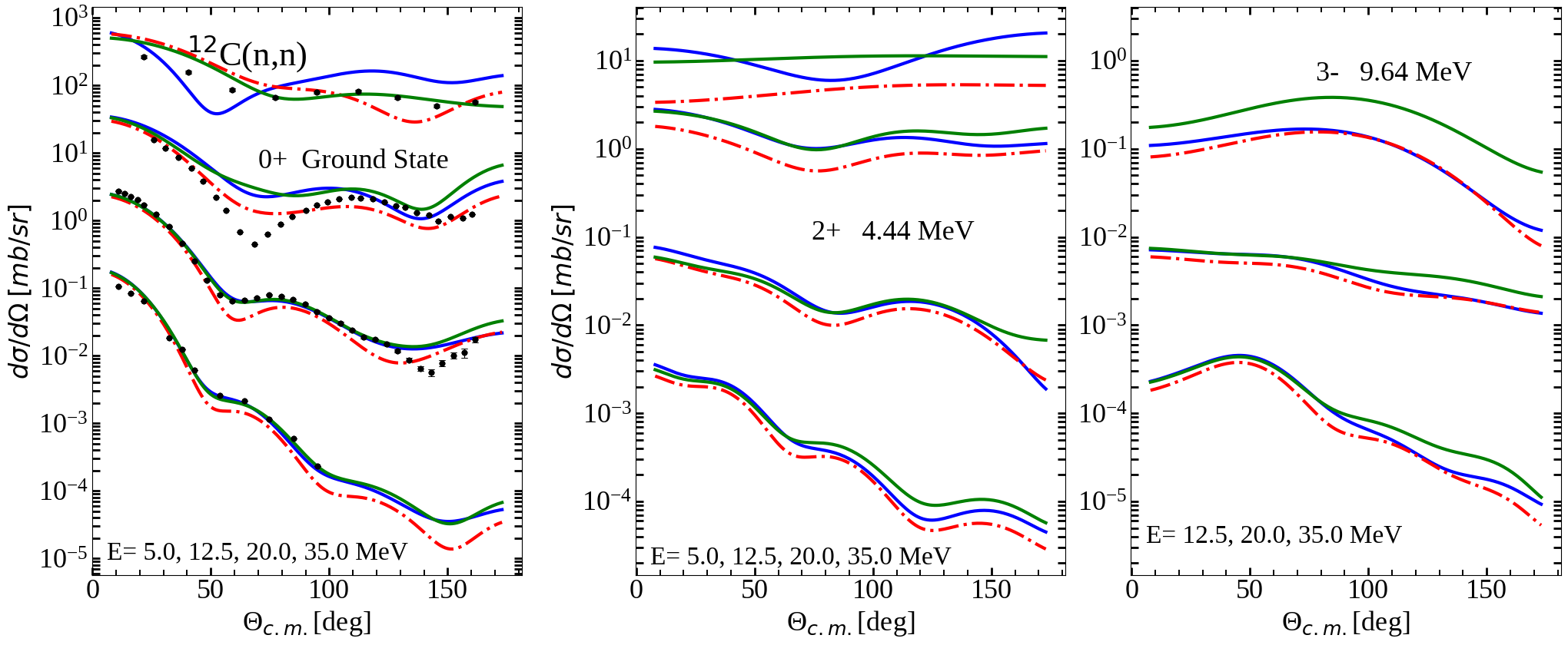
Figure 6: Differential cross-sections for a neutron on ¹²C. In all calculations the solid blue line is a calculation using the original spherical DWBA potential, the solid green line has modified that potential and uses a coupled-channel calculation. The red dashed line is the inconsistent hybrid of the original potential used in a coupled-channel environment. The left panel represents the elastic (ground state only) differential cross-section. for four different neutron energies, lowest energy at the top, highest energy at the bottom. this left panel presents one of the observables which we fit to, a good fit would be when the solid green calculation is close to the original solid blue calculation. In contrast to a proton projectile these neutron projectile calculations show more sensitivity to the modification and we are also able to show lower projectile energies due to the absence of a coulomb barrier. The central and right panel represent inelastic differential cross-sections which were not used in the fittings, they however show the sensitivity of the modification to the collective 2+ and 3- inelastic cross-sections, again the projectile energies are the lowest at the top and highest at the bottom. For more analysis see the text. For aesthetics the E=12.5 MeV cross-sections have been reduced by a factor of 20, the E= 20.0 MeV by a factor of 400, the E = 35.0 by a factor of 8000. The experimental data at E = 5.0 MeV is from Ref. [52], the data from 12.5 MeV is from Ref. [53], the data from 20.0 MeV is from Ref. [54], and the data from 35.0 MeV is from Ref. [55].

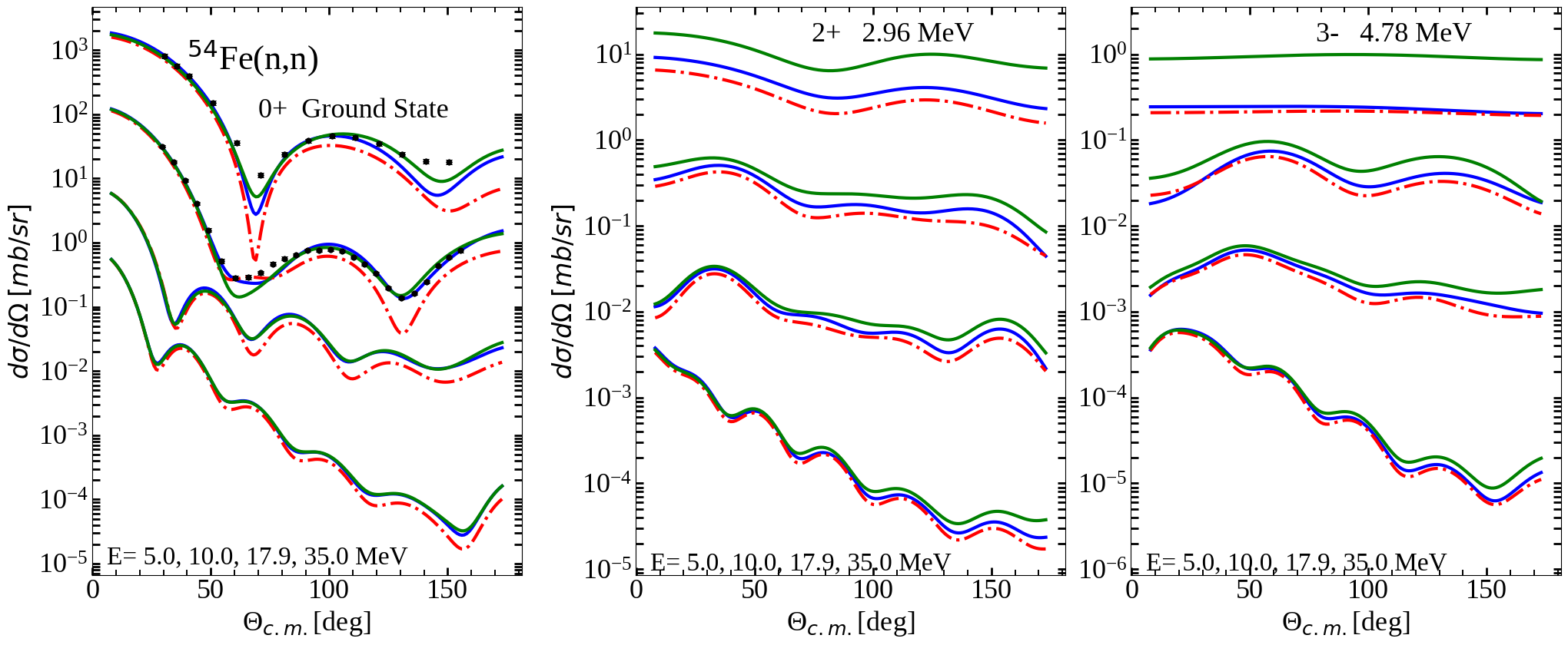
Figure 7: Differential cross-sections for a neutron on ⁵⁴Fe. The legend and description is the same as Fig. 6, for more analysis see the text. For aesthetics the E=10.0 MeV cross-sections have been reduced by a factor of 20, the E= 17.9 MeV by a factor of 400, the E = 35.0 by a factor of 8000. The experimental data from E = 5.0 MeV projectile energy is from Ref. [56], the data for E = 10.0 MeV is from Ref. [57].

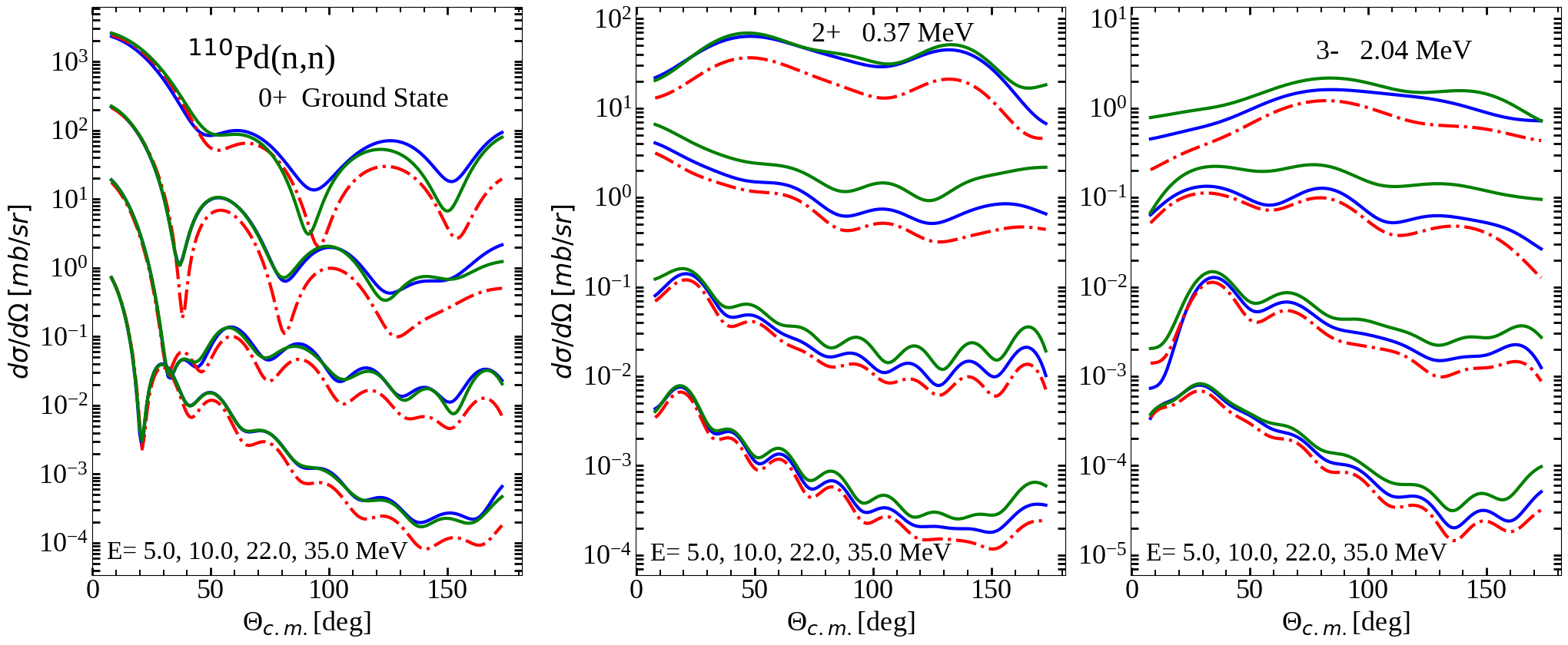
Figure 8: Differential cross-sections for a neutron on ¹¹⁰Pd. The legend and description is the same as Fig. 6, for more analysis see the text. For aesthetics the E=10.0 MeV cross-sections have been reduced by a factor of 20, the E= 20.0 MeV by a factor of 400, the E = 35.0 by a factor of 8000.

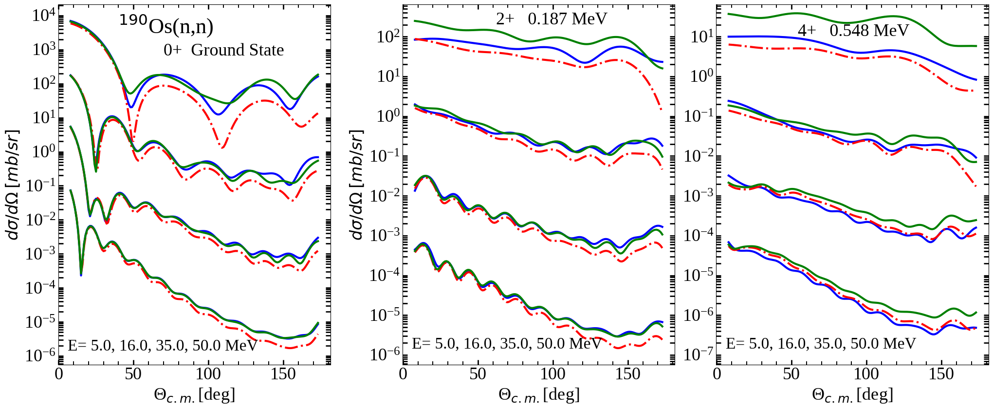
Figure 9: Differential cross-sections for a neutron on ¹⁹⁰Os. The legend and description is the same as Fig. 6, for more analysis see the text. For aesthetics the E=16.0 MeV cross-sections have been reduced by a factor of 50, the E= 35.0 MeV by a factor of 2500, the E = 50.0 by a factor of $1.25E5$.

Some systematic results that can be gleamed from the four figures of polarization graphs(10-13). As already discussed, at low energies the effects are more pronounced, thus here we displayed nothing over an energy of 65 MeV even though we calculated observables to 200 MeV. Generally, our modification to the potentials returns the optical potential to its original status (green line coincides often with blue line on the leftmost panel) even though the spin-orbit potential has only been modified in the real term’s radius and the polarization was used in fitting but in our weighted $\chi^{2}$ it had the smallest weighting. The inelastic states (the two rightmost panels of Figs. 10-13) also have systematic characteristics in that here, decisively, the calculation of our modified coupled-channel result (green solid line) coincides most often with the erroneous red-dashed line calculation which is a coupled-channel calculation which uses an inconsistent, non coupled-channel developed, potential. This signifies to us that especially at low energies, the coupled-channel aspect of the theory is an integral part of the calculation and that our modification for the inelastic spin-observables plays a secondary role.

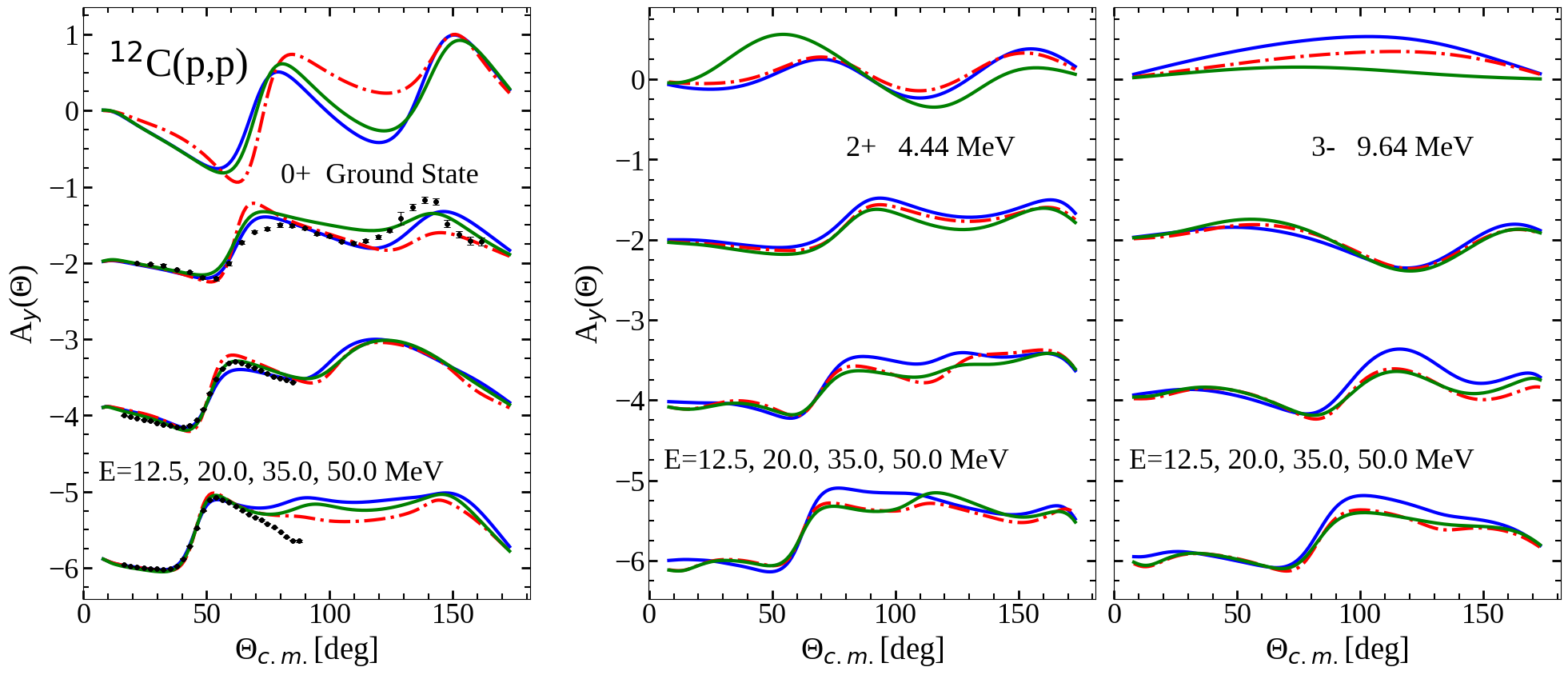
Figure 10: Spin Polarizations for a proton on ¹²C. In all calculations the solid blue line is a calculation using the original spherical DWBA potential, the solid green line has modified that potential and uses a coupled-channel calculation. The red dashed line is the inconsistent hybrid of the original potential used in a coupled-channel environment. The left panel represents the elastic (ground state only) spin polarization ($A_{y}$) for four different proton energies, lowest energy at the top, highest energy at the bottom. this left panel presents one of the observables which we fit to, a good fit would be when the solid green calculation is close to the original solid blue calculation. Note that the spin-orbit aspect of the potential was modified only in the real radius parameter and yet the fits are quite good. The central and right panel represent inelastic spin polarizations which were not used in the fittings, they however show the sensitivity of the modification to the collective 2+ and 3- inelastic cross-sections, again the projectile energies are the lowest at the top and highest at the bottom. For more analysis see the text. For aesthetics the E=20.0 MeV polarizations have been offset by a factor of -2, the E= 35.0 MeV by a factor of -4, the E = 50.0 by a factor of -6. The experimental data at E = 20.0 MeV is from Ref. [58], at 35.0 MeV and 50.0 MeV is from Ref. [59]

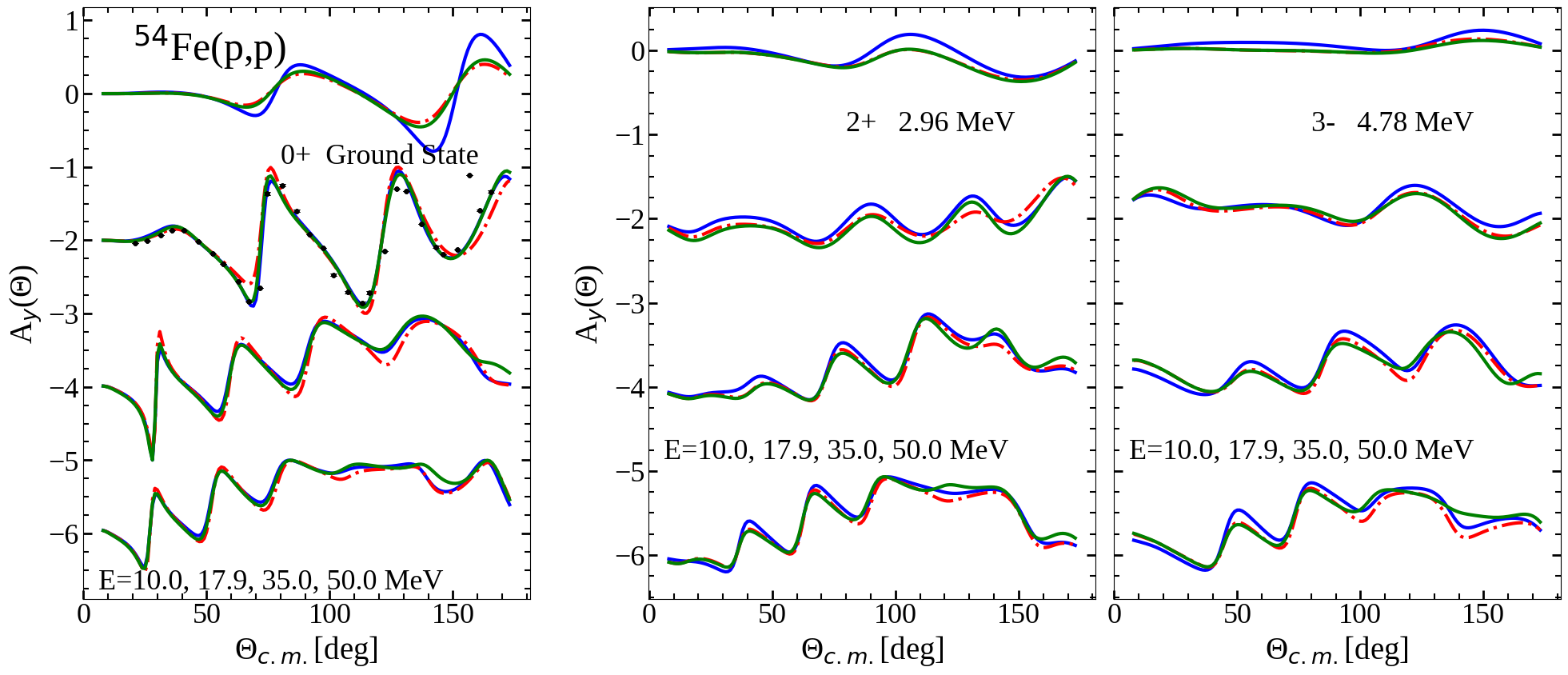
Figure 11: Spin Polarizations for a proton on ⁵⁴Fe. The legend and description is the same as Fig. 10, for more analysis see the text. For aesthetics the E=17.9 MeV polarizations have been offset by a factor of -2, the E= 35.0 MeV by a factor of -4, the E = 50.0 by a factor of -6. The experimental data at E = 17.9 MeV is from Ref. [60].

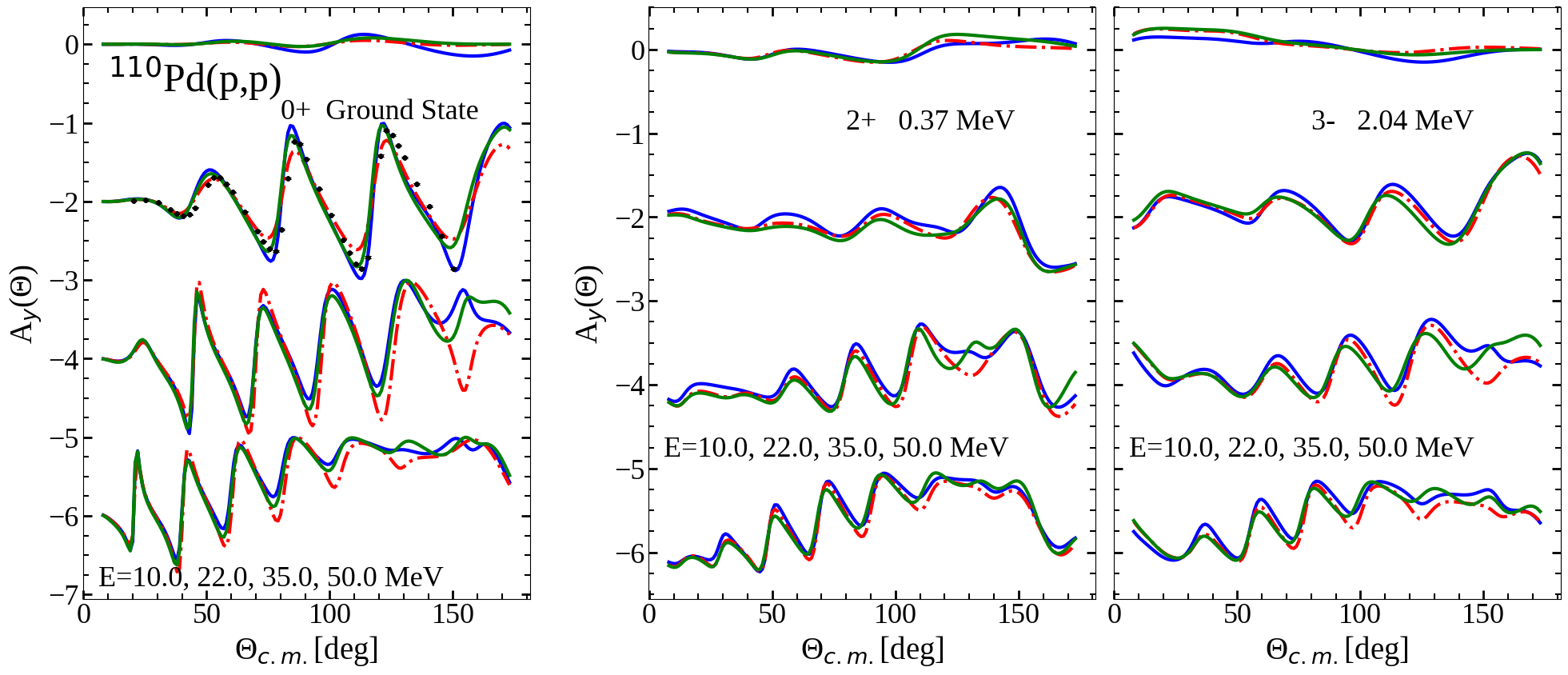
Figure 12: Spin Polarizations for a proton on ¹¹⁰Pd. The legend and description is the same as Fig. 10, for more analysis see the text. For aesthetics the E=22.0 MeV polarizations have been offset by a factor of -2, the E= 35.0 MeV by a factor of -4, the E = 50.0 by a factor of -6. The experimental data at E = 22.0 MeV is from Ref. [61].

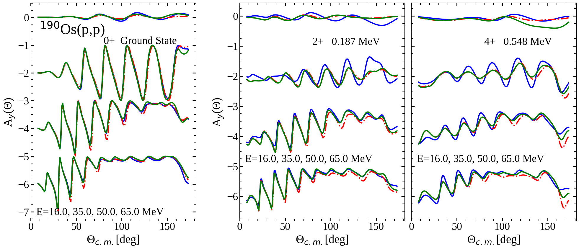
Figure 13: Spin Polarizations for a proton on ¹⁹⁰Os. The legend and description is the same as Fig. 10, for more analysis see the text. For aesthetics the E=35.0 MeV polarizations have been offset by a factor of -2, the E= 50.0 MeV by a factor of -4, the E = 65.0 by a factor of -6.

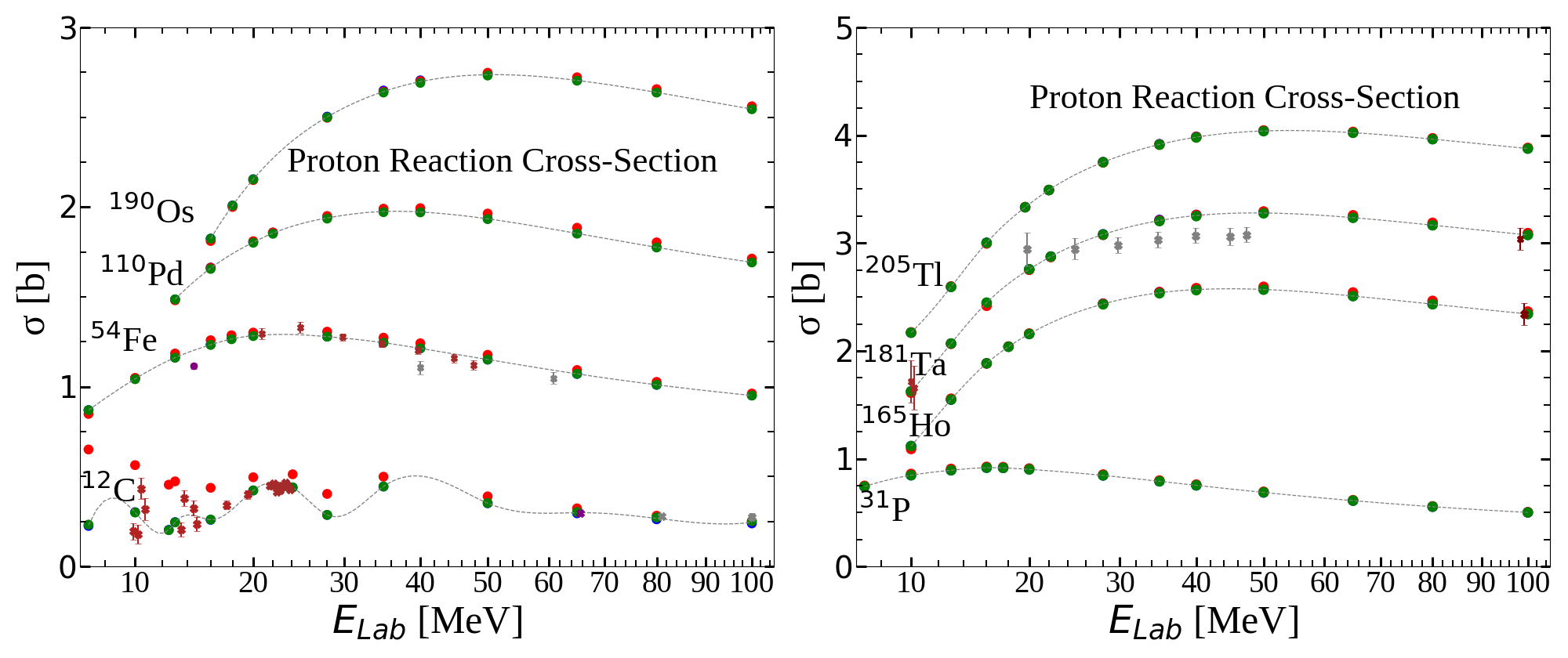
Figure 14: Eight different nuclei as targets, a proton as projectile and the total reaction (inelastic) cross-section is measured. In all calculations the solid blue circle is a calculation using the original spherical DWBA potential, the solid green circle has modified that potential and uses a coupled-channel calculation. The solid red circle is the inconsistent hybrid of the original potential used in a coupled-channel environment. The aim is to bring the modified potential (green circle) back to the original potential (blue circle). If one cannot spot the original potential calculation it is because the improved potential (green circle) is on top of it which, in this figure, is true in all cases, the fit is excellent. The thin dashed line goes through the average of the original and modified calculation to make it easy to follow the trend. For more analysis see the text. In the left panel, for aesthetic reasons, ⁵⁴Fe is offset by 250 mb, ¹¹⁰Pd is offset by 500 mb, and ¹⁹⁰Os is offset by 750 mb. In the right panel ¹⁶⁵Ho is offset by 700 mb, ¹⁸¹Ta is offset by 1330 mb, and ²⁰⁵Tl is offset by 2010 mb. Experimental data for C12 comes from Refs. [62, 63, 64, 65], the experimental data for ⁵⁴Fe comes from Refs. [66, 67, 68], the experimental data for ¹⁶⁵Ho comes from Ref. [69] and the experimental data for ¹⁸¹Ta comes from Refs. [69, 70, 71].

Lastly we look at the total cross-sections. Here we add four odd A nuclei to our study (${}^{31}P$, ${}^{165}Ho$, ${}^{185}Ta$, and ${}^{205}Tl$) because, as we shall see, the differences for the total cross-sections can be more pronounced than the differential cross-sections, more sensitivity is exhibited. That said the proton reaction cross-section is barely affected by this modification. We assume that the inelastic aspect of the coulomb force is therefore barely affected by the adjustments (this is independent on the role of the coulomb in the dipole, quadrapole, and octupole deformations). The neutron reaction cross-section does however show dramatic differences, especially at low energies. This quantity shows the error, probably the clearest of all the observables, in assuming a DWBA spherical global potential can function in a coupled-channel environment (calculation depicted by a red circle) which systematically runs high for low energy neutron scattering. This implies that the undistorted potential inflates the inelastic part of the scattering amplitude. Here we can really examine how our modification (green circle) pulls the theory back down to the original non coupled-channel calculation (blue circle). If we break our corrections into two parts: (1) the modification of the real volume amplitude and the real radius (2) the modification of the surface. Under analysis part (1) does lower this magnitude but only doing about 20% of the correction. The surface term adjustment is actually responsible for the bulk of the correction, we found this result to be true in all cases. This suggests that the altering of the radius and real volume amplitude are there to temper the change of the surface term. What we walk away understanding is that intrinsically we can mimic a distortion by shrinking the imaginary thick surface while growing the real surface term and the neutron reaction cross-section of Fig. 15 then returns to its original value. To a lesser extent we see the same behavior in the neutron total cross-section results of Fig. 16. These modifications are loosely based on theory but ultimately the algorithm chosen met the criteria that it fit these total cross-sections effectively. This is not surprising because in our weighted $\chi^{2}$ algorithm the total cross-sections were severely weighted.

The experimental results often do not coincide with either the original optical potential or its coupled modification counterpart in Fig. 16, that the fits are not ideal is common. It is difficult to fit odd nuclei, small nuclei, and low energy neutron-nucleus scattering (below 20 MeV) with an optical model ansatz. This is a reminder that the theoretical results do improve in these ranges; the adjustments do return the calculation to near their original values even though the original potential has some shortcomings. We hope that these corrections are independent of the potential and thus a good amount of work is still focused on the building of better potentials which handle the many resonances and compound states of low energy scattering (both phenomenological and microscopic). Dispersive potentials have played an important role in low energy scattering [2] and we believe that these modifications are well suited for those calculations because of only small changes to the imaginary terms.

A general statement can be made about our modifications looking at these total reaction plots (Figs. 14-16). Overall our improvements, in a coupled-channel context, lower the reaction cross-section for the nuclear force, raise the nuclear elastic cross-section (see Figs. 2-9, and thus slightly raise the total nuclear cross-section all towards the original values. As always, at low projectile energy the modification is most important.

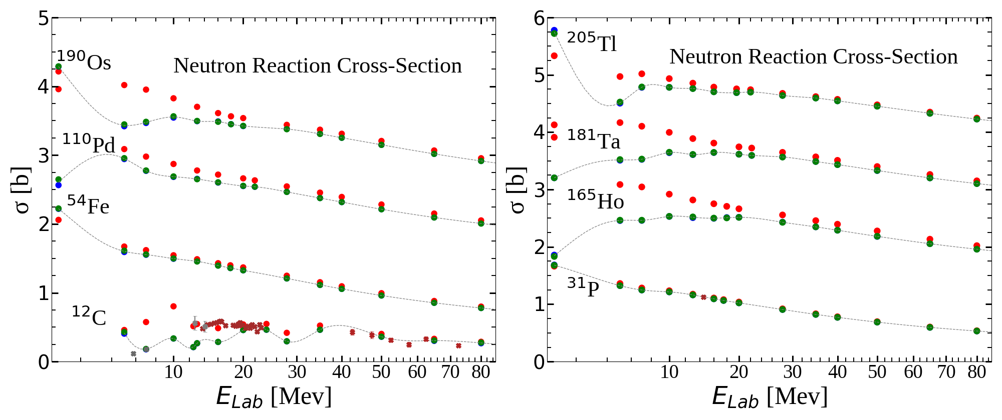
Figure 15: Eight different nuclei as targets, a neutron as projectile and the total reaction (inelastic) cross-section is measured. The legend and description is the same as Fig. 14. Note that this observable shows dramatic differences between the unmodified and the modified coupled-channel calculations, for more analysis see the text. In the left panel, for aesthetic reasons, ⁵⁴Fe is offset by 20 mb, ¹¹⁰Pd is offset by 740 mb, and ¹⁹⁰Os is offset by 960 mb. In the right panel ¹⁶⁵Ho is offset by 200 mb, ¹⁸¹Ta is offset by 1220 mb, and ²⁰⁵Tl is offset by 2190 mb. Experimental data for C12 comes from Refs. [72, 73, 74, 75], the experimental data for ${}^{31}P$ comes from Ref. [76]

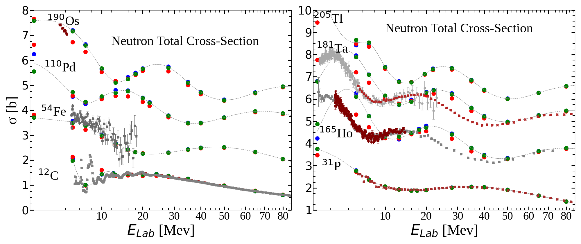
Figure 16: Eight different nuclei as targets, a neutron as projectile and the total (elastic and inelastic) cross-section is measured. The legend and description is the same as Fig. 14. Note that this observable shows dramatic differences between the unmodified and the modified coupled-channel calculations, for more analysis see the text. In the left panel, for aesthetic reasons, ¹¹⁰Pd is offset by 400 mb, and ¹⁹⁰Os is offset by 200 mb. In the right panel ¹⁶⁵Ho is offset by -700 mb, ¹⁸¹Ta is offset by 800 mb, and ²⁰⁵Tl is offset by 1700 mb. Experimental data for C12 comes from Refs. [77, 78], experimental data for ⁵⁴Fe comes from Ref. [79], and the experimental data for for ¹⁹⁰Os comes from Ref. [80].In the right panel the experimental data for ¹⁶⁵Ho comes from Refs. [81, 82], the experimental data for ¹⁸¹Ta comes from Refs. [83, 84].

Examining the change to the volume is illustrative as reflected in Fig. 17. More than 99.5% of the time the real volume of the central potential (including the surface term) grew by at most 5%. The only anomaly to this was the Carbon 12 nucleus at low energies. This was caused, we believe, because of Carbon’s extremely large distortion parameter combined with its relatively small size caused it to be unsystematic in its behavior. Historically the smaller nuclei have struggled to be fit in an optical potential ansatz. Overall, the volume stayed about the same as depicted in Fig. 17. The real central volume grew by a few percent, the imaginary central volume shrunk by a few percent. On average the magnitude of the central potential grew by 1% and, not depicted, the spin-orbit volume dropped by the same amount. As the figure depicts this was the statistical average but there were outliers. The inset of this figure shows details on our illustrative subset of target nuclei (real versus imaginary). Because of these outliers we did not make the prescription completely analytical.

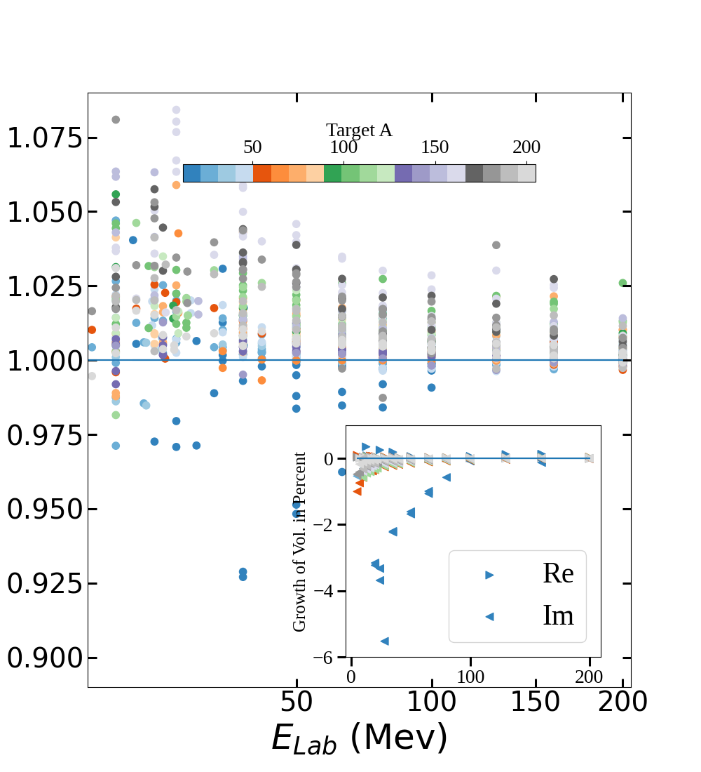
Figure 17: The main plot is a measure of how the magnitude (rms) central volume changes (in percent) when the modification is applied, this contains over a thousand points. The inset looks at a narrower set of nuclei (¹²C, ³¹P,⁵⁴Fe,¹¹⁰Pd,¹⁶⁵Ho, ¹⁸¹Ta,¹⁹⁰Os, and ²⁰⁵Tl), and shows how the imaginary volume shrank while the real volume grew.

The energy dependence of these optical potential terms has been studied [27] in the context of using coupled channels. We also see a decrease in the energy dependence of the real central amplitude and the imaginary surface amplitude but at the expense of adding a small artificial energy dependence to the real radius parameters. We applaud ways to look for lessening the energy dependence of these parameters through dispersion and/or coupled-channel techniques.

3.2 Changing the reaction and theoretical model

This method could also be applied to other DWBA local potentials which are not in the form of Woods-Saxon functions where the easiest approach would be to fit the optical potential to a Woods-Saxon basis because there is a clearly defined surface term in that space. One of the authors (S. P. Weppner) has used multiple volume and spin-orbit terms and one surface term to describe numerical microscopic local r-space potentials). There are also inelastic channels beyond collective excitations but they all involve additional parameters which, like the deformation parameter $\beta_{\lambda}$, goes to zero when that channel is closed therefore these modifications could be used in a similiar fashion with spectroscopic factors and transition potentials.

4 Conclusions

Overall we have found that if a modification is applied to a standard DWBA optical potential it then can be suitable for a coupled channel calculation which, most agree, contains relevant physics especially needed at the challenging low energy regions of less than 25 MeV. This modification was applied to a wide range of nuclei and energies and can be instantly applicable to one’s research by bringing to bear the full physical intuition of the coupled-channel approach within any form of the DWBA spherical optical potentials including the uncertainty-qualified forms [17], in fact this research could be a first step leading towards a more statistical approach. This method could also be applied to other DWBA local potential and it can be altered easily to benefit other inelastic processes (exchange, break-up, fission, fusion) and projectile scattering beyond the single nucleon all of which use the optical potential as an ingredient in their compound theory. The coupled channel environment has also been applied to a microscopic framework (see Ref. [22] for a recent review article). Likewise microscopic surface energy calculations are being studied in earnest [85, 86]. Phenomenological models, at their best, can help inform microscopic approaches and we hope the methods outlined in this research can do the same.

4.1 Acknowledgments

This research was started while one of the authors, S. P. .Weppner was on sabbatical at the Tata Institute of Fundamental Research in Mumbai. He thanks that institute and especially I. Mazumdar for their generous support.

References

References

- [1] Hebborn C, Nunes F M, Potel G, Dickhoff W H, Holt J W, Atkinson M C, Baker R B, Barbieri C, Blanchon G, Burrows M, Capote R, Danielewicz P, Dupuis M, Elster C, Escher J E, Hlophe L, Idini A, Jayatissa H, Kay B P, Kravvaris K, Manfredi J J, Mercenne A, Morillon B, Perdikakis G, Pruitt C D, Sargsyan G H, Thompson I J, Vorabbi M and Whitehead T R 2022 Optical potentials for the rare-isotope beam era URL https://arxiv.org/abs/2210.07293
- [2] Dickhoff W and Charity R 2019 Progress in Particle and Nuclear Physics 105 252–299 ISSN 0146-6410 URL https://www.sciencedirect.com/science/article/pii/S0146641018300875
- [3] Tamura T 1969 Annual Review of Nuclear Science 19 99–138 (Preprint https://doi.org/10.1146/annurev.ns.19.120169.000531) URL https://doi.org/10.1146/annurev.ns.19.120169.000531
- [4] Raynal J 2005 Phys. Rev. C 71(5) 057602 and references within URL https://link.aps.org/doi/10.1103/PhysRevC.71.057602
- [5] Thompson I J 1988 Comput. Phys. Rept. 7 167–212
- [6] Koning A and Delaroche J 2003 Nuclear Physics A 231–310 ISSN 0375-9474 URL https://www.sciencedirect.com/science/article/pii/S0375947402013210
- [7] Weppner S P, Penney R B, Diffendale G W and Vittorini G 2009 Phys. Rev. C 80(3) 034608 URL https://link.aps.org/doi/10.1103/PhysRevC.80.034608
- [8] Madland D G 1997 Progress in the development of global medium-energy nucleon-nucleus optical-model potential Proceedings of OECD/NEA Specialists Meeting on Nucleon-Nucleus Optical Model to 200 MeV p 129 this can also be found at arXiv:nucl-th/9702035v1
- [9] Becchetti F D and Greenlees G W 1969 Phys. Rev. 182 1190
- [10] Jeukenne J P, Lejeune A and Mahaux C 1977 Phys. Rev. C 15 10
- [11] Nadasen A, Schwandt P, Singh P P, Jacobs W W, Bacher A D, Debevec P T, Kaitchuck M D and Meek J T 1981 Phys. Rev. C 23 1023
- [12] Varner R L, Thompson W J, McAbee T L, Ludwig E J and Clegg T B 1991 Physics Reports 201 57
- [13] Rapaport J, Kulkarni V and Finlay R W 1997 Nucl. Phys. A 330 15
- [14] Morillon B and Romain P 2007 Phys. Rev. C 76 044601
- [15] Li X and Cai C 2008 Nucl. Phys. A 801 43–67
- [16] Whitehead T R, Lim Y and Holt J W 2021 Phys. Rev. Lett. 127(18) 182502 URL https://link.aps.org/doi/10.1103/PhysRevLett.127.182502
- [17] Pruitt C D, Escher J E and Rahman R 2023 Phys. Rev. C 107(1) 014602 URL https://link.aps.org/doi/10.1103/PhysRevC.107.014602
- [18] Nobre G P A, Palumbo A, Herman M, Brown D, Hoblit S and Dietrich F S 2015 Physical Review C 91 ISSN 1089-490X URL http://dx.doi.org/10.1103/PhysRevC.91.024618
- [19] Soukhovitskii E S, Chiba S, Lee J Y, Iwamoto O and Fukahori T 2004 Journal of Physics G: Nuclear and Particle Physics 30 905 URL https://dx.doi.org/10.1088/0954-3899/30/7/007
- [20] CAPOTE R, CHIBA S, SOUKHOVITSKIĩ E S, QUESADA J M and BAUGE E 2008 Journal of Nuclear Science and Technology 45 333–340 (Preprint https://www.tandfonline.com/doi/pdf/10.1080/18811248.2008.9711442) URL https://www.tandfonline.com/doi/abs/10.1080/18811248.2008.9711442
- [21] Soukhovitskiĩ E S, Capote R, Quesada J M, Chiba S and Martyanov D S 2016 Phys. Rev. C 94(6) 064605 URL https://link.aps.org/doi/10.1103/PhysRevC.94.064605
- [22] Hagino K, Ogata K and Moro A 2022 Progress in Particle and Nuclear Physics 125 103951 ISSN 0146-6410 URL https://www.sciencedirect.com/science/article/pii/S0146641022000126
- [23] Mackintosh R S and Keeley N 2021 Phys. Rev. C 104(4) 044616 URL https://link.aps.org/doi/10.1103/PhysRevC.104.044616
- [24] Bang J M and Vaagen J S 1980 Zeitschrift fur Physik A Hadrons and Nuclei 297 223–236
- [25] Arjan Koning Stephane Hilaire S G 2021 Talys: Comprehensive nuclear reaction modeling World Wide Web electronic publication URL https://www-nds.iaea.org/talys/
- [26] Al-Rawashdeh S M and Jaghoub M I 2018 European Physical Journal A 54 62
- [27] Al-Rayashi W S and Jaghoub M I 2016 Phys. Rev. C 93(6) 064311 URL https://link.aps.org/doi/10.1103/PhysRevC.93.064311
- [28] Weppner S P, Penney R B, Diffendale G W and Vittorini G 2014 Phys. Rev. C 89(4) 049904 URL https://link.aps.org/doi/10.1103/PhysRevC.89.049904
-
[29]
Koning A J, Hilaire S and Duijvestijn M C 2004 Talys: Comprehensive nuclear
reaction modeling Proceedings of International Conference on Nuclear
Data for Science
and Technology 769 (New York: AIP) pp 1154–1159 - [30] Raynal J 1994 Notes on ECIS94 Tech. Rep. CEA-N-2772, pp. 1–145 Commisariat ‘a l’Energie Atomique, Saclay, France
- [31] Raynal J 2006 ECIS-06 http://www.oecd-nea.org/tools/abstract/detail/nea-0850
- [32] Danielewicz P 2003 Nuclear Physics A 727 233–268 ISSN 0375-9474 URL https://www.sciencedirect.com/science/article/pii/S0375947403016622
- [33] Hasse R W and Myers W D 2012 Geometrical relationships of macroscopic nuclear physics (Springer Science & Business Media)
- [34] Jaghoub M I 2012 Phys. Rev. C 85(2) 024606 URL https://link.aps.org/doi/10.1103/PhysRevC.85.024606
- [35] Ghabar I N and Jaghoub M I 2015 Phys. Rev. C 91(6) 064308 URL https://link.aps.org/doi/10.1103/PhysRevC.91.064308
- [36] Bonaccorso A and Charity R J 2014 Phys. Rev. C 89(2) 024619 URL https://link.aps.org/doi/10.1103/PhysRevC.89.024619
- [37] Weppner S P 2018 Journal of Physics G: Nuclear and Particle Physics 45 095102 URL https://dx.doi.org/10.1088/1361-6471/aad53d
- [38] Thompson I J 2006 FRESCO http://www.fresco.org.uk
- [39] Herman M, Capote R, Carlson B, Obložinský P, Sin M, Trkov A, Wienke H and Zerkin V 2007 Nucl. Data Sheets 108 2655
- [40] Thompson I J 1988 Computer Physics Reports 7 167–212 ISSN 0167-7977 URL https://www.sciencedirect.com/science/article/pii/0167797788900056
-
[41]
Thompson I J and Nunes F M 2009 Nuclear Reactions for Astrophysics:
Principles, Calculation and Applications
of Low-Energy Reactions (Cambridge University Press) - [42] Jelley N 1990 Fundamentals of Nuclear Physics (Cambridge University Press) ISBN 9780521269940 chapter 8 URL https://books.google.co.in/books?id=7x4WXHFtBB8C
- [43] Riley L A, McPherson D M, Agiorgousis M L, Baugher T R, Bazin D, Bowry M, Cottle P D, DeVone F G, Gade A, Glowacki M T, Gregory S D, Haldeman E B, Kemper K W, Lunderberg E, Noji S, Recchia F, Sadler B V, Scott M, Weisshaar D and Zegers R G T 2016 Phys. Rev. C 93(4) 044327 URL https://link.aps.org/doi/10.1103/PhysRevC.93.044327
- [44] Möller P, Sierk A, Ichikawa T and Sagawa H 2016 Atomic Data and Nuclear Data Tables 109-110 1–204 ISSN 0092-640X URL https://www.sciencedirect.com/science/article/pii/S0092640X1600005X
- [45] Tesmer J R and Schmidt F H 1972 Phys. Rev. C 5 864–875
- [46] Gray W, Kenefick R and Kraushaar J 1965 Nuclear Physics 67 565–576 ISSN 0029-5582 URL https://www.sciencedirect.com/science/article/pii/002955826590547X
- [47] Fabrici E, Micheletti S, Pignanelli M, Resmini F G, De Leo R, D’Erasmo G, Pantaleo A, Escudié J L and Tarrats A 1980 Phys. Rev. C 21 830
- [48] Fabrici E, Micheletti S, Pignanelli M, Resmini F G, De Leo R, D’Erasmo G and Pantaleo A 1980 Phys. Rev. C 21(3) 844–860 URL https://link.aps.org/doi/10.1103/PhysRevC.21.844
- [49] Cereda E, Pignanelli M, Micheletti S, Von Geramb H V, Harakeh M N, De Leo R, D’Erasmo G and Pantaleo A 1982 Phys. Rev. C 26 1941–1959
- [50] Kruse T, Makofske W, Ogata H, Savin W, Slagowitz M, Williams M and Stoler P 1971 Nuclear Physics A 169 177–186 ISSN 0375-9474 URL https://www.sciencedirect.com/science/article/pii/0375947471905707
- [51] Svenne J P, Canton L, Amos K, Fraser P R, Karataglidis S, Pisent G and van der Knijff D 2017 Phys. Rev. C 95 034305 (Preprint 1607.04199)
- [52] White R, Lane R, Knox H and Cox J 1980 Nuclear Physics A 340 13–33 ISSN 0375-9474 URL https://www.sciencedirect.com/science/article/pii/0375947480903206
- [53] Dave J H and Gould C R 1983 Phys. Rev. C 28(6) 2212–2221 URL https://link.aps.org/doi/10.1103/PhysRevC.28.2212
- [54] Olsson N, Trostell B and Ramström E 1989 Nuclear Physics A 496 505–529 ISSN 0375-9474 URL https://www.sciencedirect.com/science/article/pii/0375947489900742
- [55] Niizeki T, Orihara H, Ishii K, Maeda K, Kabasawa M, Takahashi Y and Miura K 1990 Nuclear Instruments and Methods in Physics Research Section A: Accelerators, Spectrometers, Detectors and Associated Equipment 287 455–459 ISSN 0168-9002 URL https://www.sciencedirect.com/science/article/pii/016890029091563Q
- [56] Vanhoy J, Liu S, Hicks S, Combs B, Crider B, French A, Garza E, Harrison T, Henderson S, Howard T, McEllistrem M, Nigam S, Pecha R, Peters E, Prados-Estévez F, Ramirez A, Rice B, Ross T, Santonil Z, Sidwell L, Steves J, Thompson B and Yates S 2018 Nuclear Physics A 972 107–120 ISSN 0375-9474 URL https://www.sciencedirect.com/science/article/pii/S0375947418300307
- [57] El-Kadi S, Nelson C, Purser F, Walter R, Beyerle A, Gould C and Seagondollar L 1982 Nuclear Physics A 390 509–540 ISSN 0375-9474 URL https://www.sciencedirect.com/science/article/pii/0375947482902810
- [58] Craig R, Dore J, Greenlees G, Lowe J and Watson D 1966 Nuclear Physics 79 177–187 ISSN 0029-5582 URL https://www.sciencedirect.com/science/article/pii/0029558266904007
- [59] Ieiri M, Sakaguchi H, Nakamura M, Sakamoto H, Ogawa H, Yosol M, Ichihara T, Isshiki N, Takeuchi Y, Togawa H, Tsutsumi T, Hirata S, Nakano T, Kobayashi S, Noro T and Ikegami H 1987 Nuclear Instruments and Methods in Physics Research Section A: Accelerators, Spectrometers, Detectors and Associated Equipment 257 253–278 ISSN 0168-9002 URL https://www.sciencedirect.com/science/article/pii/0168900287907443
- [60] Van Hall P, Melssen J, Wassenaar S, Poppema O, Klein S and Nijgh G 1977 Nuclear Physics A 291 63–84 ISSN 0375-9474 URL https://www.sciencedirect.com/science/article/pii/0375947477901993
- [61] Aoki Y, Iida H, Hashimoto K, Nagano K, Takei M, Toba Y and Yagi K 1983 Nuclear Physics A 394 413–427 ISSN 0375-9474 URL https://www.sciencedirect.com/science/article/pii/037594748390115X
- [62] Dicello J F and Igo G 1970 Phys. Rev. C 2(2) 488–499 URL https://link.aps.org/doi/10.1103/PhysRevC.2.488
- [63] Šlaus I, Margaziotis D J, Carlson R F, van Oers W T H and Richardson J R 1975 Phys. Rev. C 12(3) 1093–1095 URL https://link.aps.org/doi/10.1103/PhysRevC.12.1093
- [64] Auce A, Ingemarsson A, Johansson R, Lantz M, Tibell G, Carlson R F, Shachno M J, Cowley A A, Hillhouse G C, Jacobs N M, Stander J A, Zyl J J V, Fortsch S V, Lawrie J J, Smit F D and Steyn G F 2005 Phys. Rev. C 71 064606
- [65] Ingemarsson A, Nyberg J, Renberg P, Sundberg O, Carlson R, Auce A, Johansson R, Tibell G, Clark B, Kurth Kerr L and Hama S 1999 Nuclear Physics A 653 341–354 ISSN 0375-9474 URL https://www.sciencedirect.com/science/article/pii/S0375947499002365
- [66] McCamis R H, Davison N E, van Oers W T H, Carlson R F and Cox A J 1986 Canadian Journal of Physics 64 685–691 (Preprint https://doi.org/10.1139/p86-126) URL https://doi.org/10.1139/p86-126
- [67] Dicello J F, Igo G J and Roush M L 1967 Phys. Rev. 157(4) 1001–1015 URL https://link.aps.org/doi/10.1103/PhysRev.157.1001
- [68] Menet J J H, Gross E E, Malanify J J and Zucker A 1971 Phys. Rev. C 4(4) 1114–1129 URL https://link.aps.org/doi/10.1103/PhysRevC.4.1114
- [69] Kirkby P and Link W T 1966 Canadian Journal of Physics 44 1847–1862 (Preprint https://doi.org/10.1139/p66-155) URL https://doi.org/10.1139/p66-155
- [70] Abegg R, Birchall J, Davison N, de Jong M, Ginther D, Hasell D, Nasr T, van Oers W, Carlson R and Cox A 1979 Nuclear Physics A 324 109–114 ISSN 0375-9474 URL https://www.sciencedirect.com/science/article/pii/0375947479900812
- [71] Wilkins B D and Igo G 1963 Phys. Rev. 129(5) 2198–2206 URL https://link.aps.org/doi/10.1103/PhysRev.129.2198
- [72] Ibaraki M, Baba M, Miura T, Aqki T, Hiroishi T, Nakashima H, ichiro Meigo S and Tanaka S 2002 Journal of Nuclear Science and Technology 39 405–408 (Preprint https://doi.org/10.1080/00223131.2002.10875126) URL https://doi.org/10.1080/00223131.2002.10875126
- [73] Boreli F, Kinsey B B and Shrivastava P N 1968 Phys. Rev. 174(4) 1147–1154 URL https://link.aps.org/doi/10.1103/PhysRev.174.1147
- [74] Taylor H L, Lönsjö O and Bonner T W 1955 Phys. Rev. 100(1) 174–180 URL https://link.aps.org/doi/10.1103/PhysRev.100.174
- [75] MacGregor M H and Booth R 1958 Phys. Rev. 112(2) 486–487 URL https://link.aps.org/doi/10.1103/PhysRev.112.486
- [76] Flerov N N and Talyzin V M 1957 Journal of Nuclear Energy 4 529–532
- [77] Shane R, Charity R, Elson J, Sobotka L, Devlin M, Fotiades N and O’Donnell J 2010 Nuclear Instruments and Methods in Physics Research Section A: Accelerators, Spectrometers, Detectors and Associated Equipment 614 468–474 ISSN 0168-9002 URL https://www.sciencedirect.com/science/article/pii/S0168900210000069
- [78] Abfalterer W P, Bateman F B, Dietrich F S, Finlay R W, Haight R C and Morgan G L 2001 Phys. Rev. C 63(4) 044608 URL https://link.aps.org/doi/10.1103/PhysRevC.63.044608
- [79] Cornelis E M, Mewissen L and Poortmans F 1983 Neutron resonance structure of 54fe and 56fe from high resolution total cross section experiments Nuclear Data for Science and Technology ed Böckhoff K H (Dordrecht: Springer Netherlands) pp 135–138 ISBN 978-94-009-7099-1
- [80] Hicks S E 1987 Nuclear dynamics in the shape-transitional nuclei: A study of osmium-190,192 and platinum-194,196 by neutron scattering Ph.D. thesis University of Kentucky
- [81] Marshak H, Langsford A, Tamura T and Wong C Y 1970 Phys. Rev. C 2(5) 1862–1881 URL https://link.aps.org/doi/10.1103/PhysRevC.2.1862
- [82] Foster D G and Glasgow D W 1971 Phys. Rev. C 3(2) 576–603 URL https://link.aps.org/doi/10.1103/PhysRevC.3.576
- [83] Rapp M J, Barry D P, Leinweber G, Block R C, Epping B E, Trumbull T H and Danon Y 2019 Nuclear Science and Engineering 193 903–915 (Preprint https://doi.org/10.1080/00295639.2019.1570750) URL https://doi.org/10.1080/00295639.2019.1570750
- [84] Finlay R W, Abfalterer W P, Fink G, Montei E, Adami T, Lisowski P W, Morgan G L and Haight R C 1993 Phys. Rev. C 47(1) 237–247 URL https://link.aps.org/doi/10.1103/PhysRevC.47.237
- [85] Nikolov N, Schunck N, Nazarewicz W, Bender M and Pei J 2011 Phys. Rev. C 83(3) 034305 URL https://link.aps.org/doi/10.1103/PhysRevC.83.034305
- [86] Ryssens W, Bender M, Bennaceur K, Heenen P H and Meyer J 2019 Phys. Rev. C 99(4) 044315 URL https://link.aps.org/doi/10.1103/PhysRevC.99.044315