Stream Members Only:
Data-Driven Characterization of Stellar Streams with Mixture Density Networks

Abstract

Stellar streams are sensitive probes of the Milky Way’s gravitational potential. The mean track of a stream constrains global properties of the potential, while its fine-grained surface density constrains galactic substructure. A precise characterization of streams from potentially noisy data marks a crucial step in inferring galactic structure, including the dark matter, across orders of magnitude in mass scales. Here we present a new method for constructing a smooth probability density model of stellar streams using all of the available astrometric and photometric data. To characterize a stream’s morphology and kinematics, we utilize mixture density networks to represent its on-sky track, width, stellar number density, and kinematic distribution. We model the photometry for each stream as a single-stellar population, with a distance track that is simultaneously estimated from the stream’s inferred distance modulus (using photometry) and parallax distribution (using astrometry). We use normalizing flows to characterize the distribution of background stars. We apply the method to the stream GD-1, and the tidal tails of Palomar 5. For both streams we obtain a catalog of stellar membership probabilities that are made publicly available. Importantly, our model is capable of handling data with incomplete phase-space observations, making our method applicable to the growing census of Milky Way stellar streams. When applied to a population of streams, the resulting membership probabilities from our model form the required input to infer the Milky Way’s dark matter distribution from the scale of the stellar halo down to subhalos.

1 Introduction

Stellar streams are the disrupted remnants of globular clusters and satellite galaxies, and their census has grown extensively in the Milky Way thanks to all-sky astrometric missions like Gaia (Gaia Collaboration et al., 2016a, 2023a) and low-surface brightness photometric surveys (e.g., Ibata et al. 1998; Grillmair & Dionatos 2006a; Shipp et al. 2018; Ibata et al. 2021). The formation of streams can be traced back to a progenitor (a globular cluster or satellite galaxy) whose stars are gradually lost to the tidal field of the host galaxy. The stars extend along a series of similar orbits, called tidal tails, which can sometimes span several tens of degrees across the sky. The orbital proximity of stars belonging to a stream makes them sensitive tracers of the mass distribution of galaxies, sourced by both the baryonic and dark matter components.

The average properties of a stream (e.g., the mean position and velocity track of the tidal tails) can be used to reconstruct the global dark matter distribution of the stellar halo (e.g., Johnston et al. 1999; Bonaca et al. 2014; Bovy 2014; Bovy et al. 2016; Nibauer et al. 2022; Koposov et al. 2023), while local variations in the stream track and surface density encode information about the stream’s progenitor (Küpper et al., 2012; Sanders & Binney, 2013a; Price-Whelan et al., 2014), encounters with baryonic structures such as the stellar bar (e.g., Erkal et al. 2017; Pearson et al. 2017), and non-luminous structures like dark matter subhalos (e.g., Ibata et al. 2002; Johnston et al. 2002; Carlberg 2012; Bovy et al. 2017; Bonaca et al. 2019; Hermans et al. 2021).

While several methods have been developed to model stream properties as a function of global halo characteristics (e.g., the mass distribution, flattening; Johnston et al. 1999; Binney 2008; Koposov et al. 2010; Sanders & Binney 2013b; Bovy 2014; Nibauer et al. 2022) and local substructures (e.g., the bar’s pattern speed and the mass of subhalo perturbers; Antoja et al. 2014; Hattori et al. 2016; Price-Whelan et al. 2016; Bovy et al. 2017; Pearson et al. 2017; Bonaca et al. 2019), these methods often rely on the existence of a homogenized stream-tracer population that characterizes a given stream across each of the observable phase-space dimensions. Additionally, because even the fine-grained properties of streams are influenced by the detailed mass distribution of its host galaxy, it is important to propagate errors both in measurement uncertainty and membership uncertainty (i.e., which stars belong to the stream versus the background) when attempting to model a stream. Otherwise, a poorly characterized stream could bias constraints on, e.g., the total mass of the galaxy, the dark matter halo shape, and the mass of subhalo perturbers. In order to generate more precise constraints on the structure of the galaxy, it is therefore imperative that a statistically sound and homogenized catalog of stellar streams is produced.

While streams are well described in action-angle coordinates (e.g. Bovy, 2014) or (restricted) $N$-body simulations (e.g. Dehnen et al., 2004), these methods rely on prior assumptions about the galaxy and its underlying gravitational potential. Therefore, it is necessary to devise data-driven methods to characterize stellar streams without appealing to strong prior assumptions about the galaxy’s structure.

There are a few previous works which have modeled stellar streams in this context. Patrick et al. (2022) developed the method introduced by Erkal et al. (2017), which is a data-driven, spline-based method for modeling the photometric properties and on-sky positions of previously identified streams. Their method works by fitting the stream’s stellar surface density with a series of splines, capturing both surface brightness variations along the stream and changes in the position of the stream track and width. Their method also utilizes an isochrone fit to a given stream, from which a distance modulus can be derived. While this method is very successful at characterizing the photometric properties of a stream, it does not consider the kinematic dimensions which have become increasingly well-measured with successive data releases from Gaia, as well as targeted observations. From a population of RR Lyrae stars, Price-Whelan et al. (2019) utilized a mixture model to fit the globular cluster stream Pal-5 in the space of proper motions and heliocentric distances. The mixture modeling approach enables a simultaneous fit to both the stream and background density, allowing for a cleaner selection of stream stars. However, the track of the stream in on-sky coordinates is not fit. The method identified 27 RR Lyrae stars consistent with being members of the stream. While useful for determining the average properties of a stream (e.g., its mean distance track), a limited population of RR Lyrae stars are not sufficient to capture the small-scale properties of streams expected to inform constraints on, e.g., a population of perturbers in the galaxy.

Other methods for extracting stellar streams from the data include matched-filter algorithms, where over-densities in color-magnitude space are inspected as possible clusters undergoing tidal stripping (Grillmair et al., 1995; Grillmair & Johnson, 2006; Shipp et al., 2018). While the matched-filter technique has been extremely successful in stream discovery, it is not equipped to characterize streams at the level of detail necessary to inform precise constraints on the potential of the galaxy and its substructure.

In order to address the need for a flexible model of stellar streams both in photometric and kinematic spaces, in this work we develop a new method for characterizing streams and quantifying the membership probability of possible stream stars. Our approach provides several key advantage over previous stream modeling efforts, specifically in its ability to jointly model the kinematic and photometric properties of streams simultaneously using a flexible model. Furthermore, our method is well-suited to fitting streams with only partial or incomplete phase-space or photometric observations, enabling a full characterization of streams insofar as the available data allows.

Paper organization

The paper is organized as follows. In §​ 2 we introduce our method for characterizing stream tracks and computing stellar membership probabilities. We discuss initial data processing in §​​ 2.1 and build a probabilistic framework to model the stream and background in §​​ 2.2-§​​ 2.8. In §​ 3 we apply our method to simulated data to demonstrate the model with a known ground truth dataset, then to the stellar streams GD-1 (§​ 4) and Pal 5 (§​ 5). We compare our model to other methods in §​ 6. We conclude in §​ 7, discussing the results of this work and future directions.

2 Method

Below, we offer a concise overview of our approach, followed by a more in-depth technical explanation in subsequent sections. We start, in §​​ 2.1, by transforming the astrometric data into a stream-oriented on-sky reference frame ($\phi_{1},\phi_{2},\varpi,\mu_{\phi_{1}}^{*},\mu_{\phi_{2}},v_{r})$, for each stream. In this frame, the stream track lies along $\phi_{1}$, and the stream density may be described by distributions in the other parameters as injective functions of $\phi_{1}$ (called conditional distributions). Likewise, the background of the Galactic field may be described with $\phi_{1}$-conditioned distributions. We will also model the stream in photometric coordinates. Additional features, e.g. metallicity, can also be modeled along the stream and background as functions of $\phi_{1}$, though we leave this to a future work.

The distributions for the stream and background are collected in a single mixture model that describes the entire field. We take the parameters of the mixture model — the mixture weights and component distribution parameters — to be general (continuous) functions of $\phi_{1}$, the conditioning variable. This is done using a feed-forward neural network that takes $\phi_{1}$, the conditioning variable, as its input and outputs the parameter value(s) that characterize the distribution of stars at a $\phi_{1}$ “slice”. Mixture models of conditional probability distributions using neural networks are called Mixture Density Networks (MDNs) (Bishop, 1994a). Since the model coefficients may evolve with $\phi_{1}$, MNDs are well suited to characterize streams (and the background) with all their variations in position, width, and linear density.

2.1 Framing the Data

As a stream progenitor orbits the Galactic center of mass, its path can be approximated locally as an elliptical segment. The associated arms of the stream generally align closely with its orbital plane. As viewed from a Galactocentric reference frame, the stream approximately assumes the form of a great circle enabling a 1:1 mapping from some phase parameter to a unique position along the stream. Thus in a ‘stream’ oriented frame the rotated longitudinal and latitudinal coordinates ($\phi_{1},\phi_{2}$) align with the stream such that the stream’s phase is $\phi_{1}$ and $\phi_{2}\simeq 0$.

While it would be ideal to characterize streams in this Galactocentric frame, transformation to the frame requires knowledge of the distance to the Galactic center (GRAVITY Collaboration et al., 2018; Bennett & Bovy, 2019; Leung et al., 2022), the solar motion around the Galactic center, and accurate distances to field stars (among other uncertain quantities). In a heliocentric frame, e.g. the standard ICRS (Arias et al., 1997), projection effects can obscure the shape of a stream leading to a non-trivial stream track. Therefore in a heliocentric frame, there is no assurance of effecting a rotation like in the Galactocentric frame that would similarly align the stream in an observer’s coordinates such that $\phi_{2}(\phi_{1})\approx 0$. Thankfully, most streams are adequately distant from both the Galactic center and the observer, or exhibit orientations such that a rotation a) can be established or b) holds valid. For most of the best-studied globular cluster streams – GD-1, Palomar 5, Jhelum, etc. – this holds true. However for some streams of dwarf galaxies, like the Magellanic and Sagittarius streams which each wrap around the Milky Way (Newberg et al., 2002; Majewski et al., 2003; Wannier & Wrixon, 1972), no such transformation is possible. More generally, a stream’s “sky”-projected path may be kinked, e.g. by subhalo interactions, such that it is a many-to-one function in $\phi_{1}$.

In this work we consider the vast majority of streams that can be described as an injective function, $\phi_{2}(\phi_{1})$. Since we are examining known streams this transformation is known a priori, or may be constructed during pre-processing (see Starkman et al., 2023, §2.1). We note that, with sufficient prior knowledge, many-to-one functions may be broken into injective segments and their connection constrained by a prior. Thus the methods developed here may be extended and applied even to wrapped and kinked streams. However, we leave extending the model framework to a future work.

2.2 Likelihood Setup

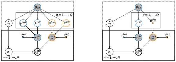
Figure 1: Probabilistic Graphical Models (PGMs) of the Mixture Density Networks used in this work. Left: A PGM of the stream model. The full dataset $x_{n}^{obs}$ is the aggregation of the observed astrometry $w_{n}^{obs}$ and photometry $m_{n}^{obs}$, along with the corresponding observational errors. We model the data as a mixture of Gaussians (in astrometry + distance modulus), with the Gaussians indexed by $q$. The weight $\alpha$ determines the weighted contribution of each Gaussian to each datum. All models are conditioned on $\phi_{1}$. Right: a PGM of the background model. The data are identical to that of the stream, however the model is not a mixture of Gaussians, but of a variety of distributions. We further distinguish between trainable distribution parameters (circles) and fixed distributions (points), like a pre-trained normalizing flow background model, explained in further detail in §​​ 2.4. Alike to the stream model, all background models are conditioned on $\phi_{1}$.

Mixture models are a statistical method to represent a population as a set of a sub-populations specified by probability distributions. These distributions are characterized by their parameters and the mixture by a corresponding set of mixture coefficients. Scalar mixture models may be extended to model completely general conditional distributions by making the distribution parameters and mixture coefficients into functions of a conditional input (McLachlan & Basford, 1989). Mixture Density Networks (MDNs) are a machine learning method to implement these general mixture models, taking the parameters and coefficients to be the outputs of feed-forward neural networks and as such, general continuous functions (Bishop, 1994b). Functional parameters allow the model to capture variation over those parameters that is not possible with scalar-valued models. Moreover, by using neural networks the inferred functional forms are “model-free” and driven entirely by the data.

For the MDN we take $x_{\cdot,0}$, the first feature column of the data $\{\mathbf{x}\}$, as the ‘independent’ coordinate over which the MDN parameters are conditioned. In the context of streams $x_{\cdot,0}\equiv\phi_{1}$ is the longitude coordinate in a reference frame rotated such that the stream is aligned along $\phi_{1}$. The parameters of the stream, the background field, and the mixing coefficients of the two are now general data-driven continuous functions along $\phi_{1}$.

The PDF of a general MDN is

$$\!\!\!p({\boldsymbol{x}}_{\mathrm{n}}|\boldsymbol{\theta}(\phi_{1}))\!=\!\sum_{\mathrm{q}\in\boldsymbol{I_{Q}}}\!{f}_{\mathrm{q}}(\phi_{1})p^{\scriptscriptstyle(q)}\left({\boldsymbol{x}}_{\mathrm{n}}|{\boldsymbol{\theta}}_{\mathrm{q}}(\phi_{1})\right),$$ (1)

where $p^{\scriptscriptstyle(q)}$ is the PDF of the $q$-th model and $f_{q}$ its mixing coefficient for all $q$ models in the set of models indexed by $\boldsymbol{I_{Q}}$. $\boldsymbol{\theta}$ is the $\phi_{1}$-conditional output of the feed-forward neural network, and ${\boldsymbol{x}}_{\mathrm{n}}$ the data on the $n$-th star in $\{\boldsymbol{x}\}$, not including $\phi_{1}$. For convenience we drop the implied subscript $n$ in $\phi_{1}$, the explicit notation of $\boldsymbol{\theta}$’s dependence on $\phi_{1}$, and the index set $\boldsymbol{I}_{X}$ in summations over its elements $x$.

The mixture coefficients ${f}_{\mathrm{q}}$ are normalized such that

$$\sum_{\mathrm{q}}{f}_{\mathrm{q}}(\phi_{1})=1,\qquad\forall\phi_{1}$$ (2)

In practice this is enforced by defining a background

$$f_{b}(\phi_{1})=1-\sum_{\rm{q}\in\boldsymbol{I_{Q}}\backslash\{b\}}{f}_{\mathrm{q}}(\phi_{1}),$$ (3)

the summation over all models except for some “background” index $b\in\boldsymbol{I_{Q}}$. In the context of Galactic streams the “foreground” is the stream itself, while the background is the Galaxy — bulge, bar, disc, halo — and additional structures, like globular clusters and dwarf galaxies, that are not associated with the stream itself. We discuss the mixture weights further in §​​ 2.5.

In this work we consider primarily astrometric and photometric data, (notated $\{\boldsymbol{w}\}$ and $\{\boldsymbol{m}\}$, respectively), but note that the MDN framework may be extended to arbitrary feature dimensions. Assuming the conditional independence of the astrometry and photometry, we split each model into linearly separable astrometric and photometric models $p^{\scriptscriptstyle(q)}=p^{\scriptscriptstyle(q,w)}p^{\scriptscriptstyle(q,m)}$.

The likelihood for a single star then becomes, simplifying from Eq. 1,

$$\!\!\!\!\!p({\boldsymbol{w}}_{\mathrm{n}},\!{\boldsymbol{m}}_{\mathrm{n}}|\boldsymbol{\theta})\!=\!\sum_{q}\!f_{q}(\phi_{1})p^{\scriptscriptstyle(q,w)}({\boldsymbol{w}}_{\mathrm{n}}|\boldsymbol{\theta})p^{\scriptscriptstyle(q,m)}({\boldsymbol{m}}_{\mathrm{n}}|\boldsymbol{\theta})$$ (4)

Assuming the measurement of each star is independent, the total log-likelihood is a sum over all stars:

$$\ln\mathcal{L}\left(\{{\boldsymbol{w}}_{\mathrm{n}},{\boldsymbol{m}}_{\mathrm{n}}\}|\boldsymbol{\theta}\right)=\sum_{n}\ln p({\boldsymbol{w}}_{\mathrm{n}},{\boldsymbol{m}}_{\mathrm{n}}|\boldsymbol{\theta}).$$ (5)

It will prove convenient to distinguish the models for $q$ as the background and stream models, respectively. In this notation:

$$p({\boldsymbol{w}}_{\mathrm{n}},{\boldsymbol{m}}_{\mathrm{n}}|\boldsymbol{\theta})= \phantom{+}\qquad f\phantom{+}p^{\scriptscriptstyle(S)}({\boldsymbol{w}}_{\mathrm{n}}|\boldsymbol{\theta})p^{\scriptscriptstyle(S)}({\boldsymbol{m}}_{\mathrm{n}}|\boldsymbol{\theta})$$ (6)

$$+(1-f)p^{\scriptscriptstyle(B)}({\boldsymbol{w}}_{\mathrm{n}}|\boldsymbol{\theta})p^{\scriptscriptstyle(B)}({\boldsymbol{m}}_{\mathrm{n}}|\boldsymbol{\theta}),$$

where we have dropped the $(w),(m)$ superscript as the model types are evident from their inputs. We applied Eq. 3 to require only a single mixture coefficient. Note that the stream and background PDFs can consist of further components. This will become important for our characterization of the stream GD-1, which appears spatially bifurcated. We note this as an implementation detail since all stream-related components (cold, extra-tidal, perturbed) and all other components (stellar halo, globular clusters, etc) may be grouped into multi-component Eq. 6 stream and background models. The stream and background models are included graphically in Fig. 1, where the left plot shows the stream model, and the right the background.

The probability of a being a stream member is then simply

$$p\!\left(S|{\boldsymbol{w}}_{\mathrm{n}},{\boldsymbol{m}}_{\mathrm{n}},\boldsymbol{\theta}\right)=\frac{fp^{\scriptscriptstyle(S)}({\boldsymbol{w}}_{\mathrm{n}}|\boldsymbol{\theta})p^{\scriptscriptstyle(S)}({\boldsymbol{m}}_{\mathrm{n}}|\boldsymbol{\theta})}{p({\boldsymbol{w}}_{\mathrm{n}},{\boldsymbol{m}}_{\mathrm{n}}|\boldsymbol{\theta})}.$$ (7)

Hereafter, when we refer to “membership probability,” Eq. 7 provides the formal definition. We nuance this definition by considering missing feature dimensions in the following subsection.

2.3 Missing Phase-Space Observations

Streams have a diversity of measurement coverage: several have full 6-D astrometrics as well as photometry and chemical abundances available (e.g., Koposov et al., 2019; Antoja et al., 2020; Li et al., 2022), while most have partial coverage, lacking some feature dimensions. Most streams detected by Gaia(Gaia Collaboration et al., 2016b, 2023b), for instance, have proper motions but not radial velocities nor high signal-to-noise parallax measurements. Follow-up surveys, like S5 (Li et al., 2019), add many feature dimensions, however only for a select set of streams. Given the diversity of coverage it is important that the likelihood model – Eq. 7 – account for missing data.

The method of treatment of missing data depends on the cause for that data to be missing. Broadly, there are two categories of causes: randomness and systematics. Consider a dataset with all features measured but with a random subset of features masked. One possible approach is to attempt to impute the missing features, then feed the full-featured data to the likelihood model. Alternatively, the likelihood model might use only the present features, ignoring those missing. If however, features are missing for systematic reasons, due to a selection function, then this approach will introduce systematic bias. The way to avoid bias where the data is incomplete due to the selection function is to know that selection function. Otherwise the probabilities will not be properly normalized. Selection functions are often very challenging to characterize, so it is routine and convenient to simply cut the data where the effects of the selection function become significant. Not including such affected data moves the contribution of the selection function from a prior to the evidence. Our models compute likelihoods under a specific dataset, and Eq. 7 is a ratio of the probabilities, so the removed selection functions are not expected to be impactful.

We adopt the approach of modeling the data masks as randomly-distributed and not systematic. We do not impute missing data, instead the per-star likelihood is modeled with a distribution with the same dimensionality as the data vector. For example, a star with a 6D astrometric measurement will be modeled with a full 6D distribution, while a star missing its radial velocity measurement will be modeled with a dimensionally-reduced (5D) form of the 6D distribution. Using dimensionally reduced distributions ensure that missing phase-space dimensions do not amplify nor suppress the likelihood. Notwithstanding, we include a quality flag on our calculations indicating the number of missing features. We leave incorporating priors on the data mask distribution to future work.

2.4 Pre-training distributions

In §​​ 2.2 we set up the general mathematical framework of MDNs, then specified the models on two axes: the component and the data type. Broadly, the components are stream versus background and the data types are astrometric and photometric. For some components, e.g. the stream, the data density will be well fit by an analytic function. For others, no analytic density provides a realistic description of the data. In this work we take a data-driven approach, and represent non-analytic distributions using a normalizing flow model.

Normalizing flows provide a flexible description of a probability density, by transforming samples generated from a simple base distribution (i.e., a Gaussian) to the more complicated target distribution (Tabak & Vanden-Eijnden, 2010; Rippel & Prescott Adams, 2013; Jimenez Rezende & Mohamed, 2015). The transformations are typically non-linear outputs of a neural network, whose parameters are optimized until the target density accurately characterizes the data. The neural network transformation is differentiable, so that jacobian factors can be combined to ensure that the target distribution remains a valid probability density (i.e., integrates to one) (Kobyzev et al., 2019). For the neural networks we regularize the data (minus the mean, divided by the standard deviation per feature column); thus we correct the overall normalization of the flow by the product of the jacobian of the regularization operation.

Our implementation is as follows. For a given stream, we restrict the data to some field characterized by a polygon drawn around the stream. Because our density modeling is aimed at stream characterization rather than discovery, we assume that the stream is sufficiently well known so that it can be masked out as a simple cut in (e.g.) $\phi_{1}-\phi_{2}$ coordinates. With the stream masked out, we then fit a normalizing flow to the data. Because the distribution can evolve with $\phi_{1}$, we fit a conditional normalizing flow, $q_{\rm flow}(\mathbf{x}|\phi_{1})$. Our central assumption with this model is that the distribution for background stars in the masked region are quantitatively similar to those in the unmasked region. For a sufficiently narrow mask we expect this to be the case, and find that this assumption does not introduce bias for the streams considered in this work.

Once the normalizing flow, $q_{\rm flow}\left(\mathbf{x}|\phi_{1}\right)$, is fit to the data, its parameters are fixed while the other components of the model begin training. Therefore, the normalizing flow can be rapidly trained and computed as a pre-processing step.

It is easy to evaluate the log-likelihood of a normalizing flow at a point $\boldsymbol{x}$ when all feature dimensions are present. When one (or more) feature dimension is missing, however, evaluating the marginal log-likelihood involves integrals over the flow. While the procedure is straightforward it is computationally expensive. As an alternative, we conservatively set the log-likelihood to $0$, the maximum value, overemphasizing the flow’s contribution to the background model. Conceptually, up-weighting the background model decreases the false-positive rate in stream membership identification, at the cost of increasing the false-negative rate. Another approach, which we leave to a future work, is to construct normalizing flows of each marginal distribution, e.g. $q_{\rm flow}\left(\{x_{i}\}_{i\in\boldsymbol{I}_{F},i\neq{j,k}}|x_{j},x_{k},\phi_{1}\right)$, and select for each ${\boldsymbol{x}}_{\mathrm{n}}$ the correct flow given the present features.

2.5 Determination of the Mixture Weight

The mixture weight $f_{q}(\phi_{1})$ as used in Eq. 4 is characterized as the fraction of stars belonging to the mixture component $q$ over an increment $[\phi_{1},\phi_{1}+\mathrm{d}{\phi_{1}}]$. Thus, the mixture weight encodes information about the linear density of the stream, which has been shown to depend on substructure in the galaxy (Siegal-Gaskins & Valluri, 2008; Yoon et al., 2011). The dependence of the mixture weight on the linear density is captured by the expression

$$f_{q}\left(\phi_{1}\right)=\frac{n_{q}\left(\phi_{1}\right)}{n_{\rm tot}\left(\phi_{1}\right)},$$ (8)

where $n_{q}\left(\phi_{1}\right)$ is the number density of stars in component $q$ (i.e., the number of stars belonging to component $q$ per $\phi_{1}$ interval), and $n_{\rm tot}$ is the total number density of stars in the same interval (including those in component $q$). The linear density for component $q$ is then entirely specified by the function $n_{q}(\phi_{1})$.

The mixture model specified in Eq. 4 only models the weight parameter $f_{q}$, and not the components of the ratio in Eq. 8. However, the linear density $n_{q}(\phi_{1})$ can be readily obtained from $f_{q}$, provided that $n_{\rm tot}\left(\phi_{1}\right)$ can be calculated. Importantly, this function does not depend on the parameters of the on-stream or off-stream model. Instead, $n_{\rm tot}(\phi_{1})$ is simply proportional to the number of stars in a small $\phi_{1}$ increment. We therefore model $n_{\rm tot}\left(\phi_{1}\right)$ as a post-processing step using a single normalizing flow in $\phi_{1}$.

In particular, for a given field the distribution of $\phi_{1}$ coordinates is specified by the set $\{\phi_{1}\}_{f}$. A normalizing flow is trained to this dataset, and will satisfy $\int d\phi_{1}P_{\phi_{f}}(\phi_{1})=1$ by construction. We can then obtain the linear stream density with

$$n_{q}\left(\phi_{1}\right)=f_{q}\!\left(\phi_{1}\right)\,n_{\rm tot}\!\left(\phi_{1}\right)\equiv f_{q}\!\left(\phi_{1}\right)P_{\phi_{1}}\!\!\left(\phi_{1}\right).$$ (9)

2.6 Astrometric Model

2.6.1 On-Stream

The N-dimensional astrometric track is modeled with a single neural network, parameterized as a function of $\phi_{1}$. The neural network output for a single stream component is the mean location of the stream track in each dimension, ${\boldsymbol{\mu}}_{w}(\phi_{1})$, and its associated covariance matrix ${\boldsymbol{\Sigma}}_{w}(\phi_{1})$. The probability for the data is then

$$p^{\scriptscriptstyle(S,w)}({\boldsymbol{w}}_{\mathrm{n}}|\boldsymbol{\theta})\!=\mathcal{N}_{F}\big{(}{\boldsymbol{w}}_{\mathrm{n}}|{\boldsymbol{\mu}}_{w}\!(\phi_{1}),{{\boldsymbol{\Sigma}}_{\mathrm{n}}^{\scriptscriptstyle(w)}}^{2}\!+\!{\boldsymbol{\Sigma}}_{w}^{2}\!\left(\phi_{1}\right)\!\big{)},$$ (10)

where ${\boldsymbol{\theta}}_{w}$ is the set of neural network parameters that define ${\boldsymbol{\mu}}_{w}$ and ${\boldsymbol{\Sigma}}_{w}$; and ${\boldsymbol{\Sigma}}_{\mathrm{n}}^{\scriptscriptstyle(w)}$ the data uncertainties. In the simplest case, we take ${\boldsymbol{\Sigma}}_{\mathrm{n}}^{\scriptscriptstyle(w)},{\boldsymbol{\Sigma}}_{w}$ to be diagonal, consisting of both intrinsic dispersion for each dimension of $\boldsymbol{w}$ and the data uncertainties added in quadrature. The data uncertainties ${\boldsymbol{\Sigma}}_{\mathrm{n}}^{\scriptscriptstyle(w)}$ are elements of $\boldsymbol{\delta}\mathbf{W}$, the dataset of astrometric uncertainties.

In practice, we work with truncated Gaussians, where the truncation is set by the size of the field in each astrometric dimension. Details of the truncated Gaussian are included in §​​ A.3. Truncating to the field ensures that the probability density is zero wherever there is no data. This has an added benefit of correctly normalizing the Gaussian distribution, which is not compact (has non-zero probability over all space) and would otherwise not integrate to one within the field.

As a MDN, we implement the Gaussian distribution parameters with a multi-layered feed-forward neural network. The number of layers required depends on the maximum dimensionality of the Gaussian, and whether the neural network employs regularization techniques like dropout. We use alternating layers of linear and tanh units. Details of the network architecture are discussed in §​​ 2.9.

If a particular observation has missing phase-space coordinate(s) $f_{k}$, we reduce the dimensionality of the Gaussian to that of the data-vector. Namely, for $\boldsymbol{I}_{\tilde{F}}\equiv\boldsymbol{I}_{F}\backslash\{f_{k}\}$

$${\tilde{\mathbf{w}}}_{\mathrm{n}} \mapsto{\tilde{\mathbf{w}}}_{\mathrm{n}}=\{w_{n,f}|f\in\boldsymbol{I}_{\tilde{F}}\},$$

$${\boldsymbol{\mu}}_{w} \mapsto{\tilde{\boldsymbol{\mu}}}_{w}=\{\mu_{f}|f\in\boldsymbol{I}_{\tilde{F}}\},$$

$${\boldsymbol{\Sigma}}_{w} \mapsto{\tilde{\boldsymbol{\Sigma}}}_{w}=\{\Sigma_{i,j}|i,j\in\boldsymbol{I}_{\tilde{F}}\},$$

such that,

$$p^{\scriptscriptstyle(S)}({\boldsymbol{w}}_{\mathrm{n}} |{\boldsymbol{\theta}}_{w}(\phi_{1}))\mapsto p^{\scriptscriptstyle(S)}({\tilde{\boldsymbol{w}}}_{\mathrm{n}}|{\tilde{\boldsymbol{\theta}}}_{w}(\phi_{1}))\,.$$ (11)

2.6.2 Off-stream

We now outline the off-stream astrometric model. We take a similar approach to the on-stream astrometric model discussed in §​ 2.6.1, though we typically do not characterize the backgrounds with a Gaussian distribution. Instead, we utilize a range of distributions (i.e., exponential, skew-normal) discussed in Appendix A. The parameters of the user-specified background distributions are themselves neural network outputs, such that any $\phi_{1}$ “slice” of the background should be characterized by some analytic density, but the evolution of the backgrounds with $\phi_{1}$ can be complex. Details of the network architecture are discussed in §​​ 2.9.

Let ${\boldsymbol{\theta}}_{\mathrm{f}}^{\scriptscriptstyle(B)}(\phi_{1})$ represent the neural network which outputs a vector of parameters characterizing the background distribution at a given $\phi_{1}$ for astrometric dimension $f$. The number of outputs for the background model is equal to $\mathrm{dim}\left({\boldsymbol{\theta}^{\scriptscriptstyle(B)}}_{\mathrm{f}}\right)$ (where $f=0$ corresponds to $\phi_{1}$, which we do not model). At a given $\phi_{1}$, the probability density for the astrometric dimension $f>0$ is ${p}_{\mathrm{f}}^{\scriptscriptstyle(B)}\left(\boldsymbol{w}_{n,f}|{\boldsymbol{\theta}}_{\mathrm{f}}^{\scriptscriptstyle(B)}(\phi_{1})\right)$. We treat each background component dimension as independent, allowing us to write the likelihood as a product over the astrometric dimensions:

$$p^{(B)}\left({\boldsymbol{w}}_{\mathrm{n}}|\boldsymbol{\theta}(\phi_{1})\right)=\prod_{f\in\boldsymbol{I}_{\tilde{F}}}p_{f}^{(B)}\left(\boldsymbol{w}_{n,f}|{\boldsymbol{\theta}}_{\mathrm{f}}^{\scriptscriptstyle(B)}(\phi_{1})\right)\,,$$ (12)

where $\boldsymbol{I}_{\tilde{F}}$ is the set of indices of the features, omitting missing phase space dimensions.

2.7 Photometric Model

2.7.1 On-Stream

In photometric coordinates we model the stream as a single-population isochrone with the possibility of a non-zero distance gradient. We accomplish this by modeling the distance of the isochrone as a neural network output, parameterized as a function of $\phi_{1}$. The result is a distance track along the stream, estimated from the variation in its isochrone with $\phi_{1}$.

At any given $\phi_{1}$, the isochrone is modeled in absolute magnitudes and parameterized by the normalized stellar mass, labeled $\gamma\in(0,1]$, in the modeled mass range. For example, increasing $\gamma$ corresponds to movement up the main sequence towards the red giant branch. We denote the isochrone as $\mathcal{I(\gamma)}$, and StreamMapper permits any such distribution. The intrinsic dispersion around the isochrone is $\Sigma_{\mathcal{I}}(\gamma)$. Since the isochrone is in absolute magnitudes, but the data are in apparent magnitudes, it is necessary to shift the isochrone by a distance modulus to the predicted distance of the stream, labeled $\mu(\phi_{1})$, with intrinsic stream distance variation $\sigma_{\mu}(\gamma)$.

For the $n$-th star, the photometric model is:

$$p^{\scriptscriptstyle(S,m)}(\boldsymbol{m_{i}},\gamma|\boldsymbol{\theta}(\phi_{1}))\\ \sim\mathcal{N}({\boldsymbol{m}}_{\mathrm{n}}|\{\mathcal{I(\gamma)}+\mu(\phi_{1}),\boldsymbol{\Sigma}_{\mathcal{I}}^{2}(\gamma)+\mathds{1}\sigma_{\mu}^{2}(\phi_{1})+{{\boldsymbol{\Sigma}}_{\mathrm{n}}^{\scriptscriptstyle(m)}}^{2}\})\\ \times\mathcal{\pi}(\gamma,{\boldsymbol{m}}_{\mathrm{n}},\phi_{1}),$$ (13)

where ${\boldsymbol{\Sigma}}_{\mathrm{n}}^{\scriptscriptstyle(m)}$ is the data covariance and $\mathcal{\pi}(\gamma,{\boldsymbol{m}}_{\mathrm{n}},\phi_{1})$ encodes both the present-day mass function of the stream, as well as any observational constraints (e.g., $g<20$ mag).

For a given star, we are interested in its probability of belonging to the stream’s isochrone. Therefore, we marginalize over $\gamma$ to find:

$$p^{\scriptscriptstyle(S,m)}({\boldsymbol{m}}_{\mathrm{n}}|\boldsymbol{\theta}(\phi_{1}))=$$ (14)

$$\ \int\limits_{\gamma=0}^{1}\mathcal{N}({\boldsymbol{m}}_{\mathrm{n}}|\{\mathcal{I(\gamma)}+\mu(\phi_{1}),\boldsymbol{\Sigma}_{\mathcal{I}}^{2}(\gamma)+\mathds{1}\sigma_{\mu}^{2}(\phi_{1})+{{\boldsymbol{\Sigma}}_{\mathrm{n}}^{\scriptscriptstyle(m)}}^{2}\})$$

$$\qquad\times\mathcal{\pi}(\gamma,{\boldsymbol{m}}_{\mathrm{n}}|\phi_{1})\rm{d}\gamma.$$

Then, for a given $\phi_{1}$ we can obtain a distribution over the distance modulus using

$$\mu_{\rm sample}\left(\phi_{1}\right)\sim\mathcal{N}\left(\mu(\phi_{1}),\sigma^{2}_{\mu}(\phi_{1})\right).$$ (15)

For each sample, we can convert the distance-modulus distribution (and error) to the distance track using

$$\rm{dist}\left(\phi_{1}\right) =10^{\frac{1}{5}\mu_{\rm sample}(\phi_{1})+1} \quad[\text{pc}],$$ (16)

$$\delta\rm{dist}(\phi_{1}) \simeq\frac{\ln{10}}{5}\rm{dist}(\phi_{1})\ \sigma_{\mu}(\phi_{1}) \quad[\text{pc}].$$ (17)

Let $\boldsymbol{\theta}^{\scriptscriptstyle(S,m)}(\phi_{1})$ represent the feed-forward neural network which outputs a vector of parameters characterizing the stream’s photometric distribution at a given $\phi_{1}$. The network has 2 outputs – $\mu,\sigma_{\mu}$ – as we only consider the distance track of the isochrone, holding fixed stellar population parameters internal to modeling the isochrone, such as its age and metallicity. In principle we might include parameters of the isochrone in the model, now $\mathcal{I}(\boldsymbol{\theta},\gamma)$, where $\theta={a,Z,...}$ and any other generating parameters of the isochrone. However, at a detailed level stellar streams are generally poorly fit by theoretical isochrones, at least ones with realistic ages and metallicities. Consequently including the age and metallicity as model parameters does not meaningfully contribute to constraining results on the stream’s stellar population. Moreover, age and metallicity are partially degenerate with the distance modulus, working counter to the goal of fitting a distance track to the stream. An alternate approach is to use data-driven isochrones instead of theoretic ones. StreamMapper allows any isochrone from any theoretic or data-driven library to be used, so long as the isochrone may be described as a curve $\mathcal{I}(\gamma,\phi_{1})$ with dispersion $\Sigma_{\mathcal{I}}(\gamma,\phi_{1})$. In this work we use MIST (Dotter, 2016; Choi et al., 2016) isochrones for their convenience, but recognize their limitations as compared to data-driven isochrones. We defer using data-driven isochrones and constraining ages and metallicities to a future work.

The photometric probability, Eq. 14, encodes the photometric distribution – the “track” – of the isochrone model, as well as the relative probability of points along the track. The latter is the term $\mathcal{\pi}(\gamma,{\boldsymbol{m}}_{\mathrm{n}}|\phi_{1})$, which describes all priors on both the isochrone as well as survey constraints and selection effects. We assume that the properties of the isochrone are conditionally independent from observational constraints; namely

$$\mathcal{\pi}(\gamma,{\boldsymbol{m}}_{\mathrm{n}}|\phi_{1})=\mathcal{\pi}_{\cal{I}}(\gamma|\phi_{1})\mathcal{\pi}_{obs}({\boldsymbol{m}}_{\mathrm{n}}|\phi_{1})$$ (18)

where $\mathcal{\pi}_{\mathcal{I}}$ and $\mathcal{\pi}_{obs}$ are the isochrone and observational priors, respectively.

The second term in Eq. 18 – $\mathcal{\pi}_{obs}({\boldsymbol{m}}_{\mathrm{n}}|\phi_{1})$ – encodes all observational effects in the photometric dataset. Some effects are easily modeled, e.g. instruments have well-characterized magnitude limits, both faint and bright. Other effects are not easily modeled, e.g, complex location-dependent completeness issues (Gaia Collaboration, 2023). Accounting for the completeness is very challenging. In practice we avoid the contribution of completeness to $\mathcal{\pi}_{obs}$, masking data for which it is relevant. Gaia, for instance, is complete from $12<G<17$ and has high completeness up to $G\approx 20$, thus we mask $G>20$. The masks are easily modeled as magnitude limits and replace the complex completeness model in $\mathcal{\pi}_{obs}$. §​​ 2.3 explains how masking is implemented in the models, though in this case every feature is masked, not only a few feature dimensions. With every featured masked, the photometric model in Eq. 14 reduces from an $F_{m}$-dimensional Gaussian to a 0-D Gaussian, which is a null distribution and does not enter into the likelihood. In photometric coordinates completeness depends on a stars apparent magnitude; viewed in astrometric coordinates, the completeness cannot be described so simply. Gaia, for instance has scanning law residuals in the density field. When photometric coordinates are masked due to completeness, we do not mask the corresponding astrometric features, so that the stars membership probability is determined solely by the astrometric model. This practice allows us to include stars with good astrometric measurements, not penalizing those stars for which the photometric model is insufficient. We examine the results to confirm that the scan pattern does not impact the membership distribution.

The first term in Eq. 18 – $\mathcal{\pi}_{\mathcal{I}}$ – encodes the point-wise amplitude of the isochrone. Physically, this amplitude is the the present-day mass function (PDMF). The PDMF $\mathcal{\pi}_{\cal{I}}(\gamma,\phi_{1})$ is a joint distribution, depending on $\gamma$ since it is the $\gamma$-dependent distribution amplitude, and also on $\phi_{1}$. This latter dependence is confusingly termed the “mass function of the stream”, which is the expected variation in the stellar mass distrubion along the stream, arising due to e.g. mass segregation in the progenitor (Webb & Bovy, 2022). To date this variation along the stream has not been observed, so in practice we drop the $\phi_{1}$ dependence – $\mathcal{\pi}_{\cal{I}}(\gamma,\phi_{1})=\mathcal{\pi}_{\cal{I}}(\gamma)$ – assuming that the PDMF is constant along the stream.

In the StreamMapper we offer a few ansatz for the PDMF, though any user-defined function may be used instead. The default assumption, known to be non-physical, is a uniform distribution over $\gamma$. Similarly non-physical are truncated uniform distributions, considering only a segment of the isochrone, e.g. the main sequence turnoff (MSTO). We include also a Kroupa initial mass function (IMF) (Kroupa, 2001). The Kroupa IMF, and all physically-motivated IMFs, have a much larger fraction of low-mass stars than high-mass stars, the latter being less likely to form. This is observed in streams, particularly their progenitors. However the Kroupa IMF, and most out-of-the-box IMFs, are poor fits to the observed PDMF as stream progenitors like globular clusters are extremely old ($\sim 10$ Gyr) and may be dynamically evolved (Grillmair & Smith, 2001) while an IMF is the zero-age distribution. How then should the PDMF $\mathcal{\pi}_{\cal{I}}$ be treated? One approach to the PDMF is to use a more informed distribution, for example time-evolving an IMF, either analytically or by simulation, to the age of the stream’s stellar population. However, for many streams, e.g. those lacking known progenitors, the PDMF is observationally poorly constrained. In short, using any fixed distribution is simple in implementation, however the choice of distribution is not.

Rather than using a fixed a priori ansatz, another approach to the PDMF is to incorporate it into the model, parameterized by some distribution and fit simultaneously to the distance modulus and other $\boldsymbol{\theta}^{\scriptscriptstyle(m)}$. We find this, like incorporating $a,Z$ into the isochrone model, to be interesting avenues by which to develop the model. However the resulting significant increase in model flexibility necessitates careful regulation, and we leave this to a future work.

The last approach to the issue of the PDMF, and the one we take in this work, is to render it unimportant. With fixed age, metallicity, and other isochrone model parameters, the primary purpose of the isochrone is to allow the model to determine the distance modulus of the stream. For this, only a portion of the stream need be modeled. For streams with observable main sequence turn-offs, like GD-1 in Gaia, this portion of the isochrone has both many stars and a relatively small range in masses. Thus, we restrict the mass range of the isochrone such that we are modeling only a region of interest over which the PDMF does not meaningfully contribute to the final result.

2.7.2 Linking to Astrometrics: the Distance Modulus and the Parallax

By modeling jointly the astrometrics and photometrics we may tie together components of the models. In particular, the distance modulus in the photometric model and the parallax in the astrometric model are both measures of the distance track of the stream. We model in the same coordinates as the data, and thus prefer parallax and distance modulus over the distance for each model type. We introduce a prior to connect these components of the models:

$$\mathcal{\pi}(\{\mu_{I},\mu_{\varpi}\}|\phi_{1}) =\delta(\rm{dist}(\mu_{I})-\rm{dist}(\varpi))(\phi_{1}),$$ (19)

where $\delta$ is the Dirac delta function (Dirac, 1947), and enforces that the distance modulus track and parallax track must be equal (when converted to the actual distance) as a function of $\phi_{1}$. The widths are similarly constrained. The distance and first-order error conversion are given by

$$\mu_{I}(\varpi) =10-5\log_{10}(\varpi)$$ (20)

$$\sigma_{I}(\sigma_{\varpi}) \approxeq\frac{5}{\ln{10}}\mu_{I}\lvert\sigma_{\varpi}\rvert.$$ (21)

In practice, at the distance of many streams the errors in the parallaxes are of order 1 and we exclude the feature from the model.

2.7.3 Off-stream

The distribution of background stars in color (i.e., $g-r$) and magnitude (i.e., $g$) is a complicated function of location in the galaxy. Even within a field centered on the stream of interest, the color-magnitude diagram (CMD) is a combination of stellar populations distributed over a range in distances. Because of this, we do not find an analytic density that describes the data and use instead a normalizing flow, discussed in §​​ 2.4. Because the background CMD can evolve with $\phi_{1}$, we fit a conditional normalizing flow, $q_{\rm flow}(\mathbf{m}|\phi_{1})$, so that the color-magnitude diagram is conditionally dependent on position along the stream. In practice, we model magnitudes and not colors (i.e., $\mathbf{m}=(g,r)$ rather than $g\ \mathrm{and}\ g-r$. Otherwise, the two arguments will always be covariate). The normalizing flow approach makes modeling the photometry relatively straightforward.

In photometry the intrinsic width of stellar streams tends to be quite small, with correspondingly small $\sigma_{\mu}$ (see Eq. 14). Therefore the effective region of the isochrone model is well determined and we do not find the marginal log-likelihood approach discussed in §​​ 2.4 to be impactful.

2.8 Priors

In §​​ 2.2 we introduced the likelihood setup. In §​ 2.7.1 we added priors in the form of the isochrone’s PDMF and photometric observational constraints. In this section we introduce and develop more priors that are important for training our Bayesian Mixture Density Network.

2.8.1 Parameter Bounds

For each parameter in $\boldsymbol{\theta}$ of the model we implement priors on its range. Uninformative, e.g. uniform $\mathcal{U}(a,b)$, priors are often assumed where little is known about a parameter (except that $(a,b]$ contain the correct $\theta$ and its distribution). Where more is known about $\theta$, for instance that it is a categorical, more informative priors like the Dirichlet distribution (Bishop, 2016) may be used. Our code, StreamMapper, permits any user-defined prior, and we include $\mathcal{U}(a,b)$. The default choice of prior and bounds $\mathcal{U}$ set to the limits of the dataset in each feature dimension.

We implement a hard-coded uniform prior on a neural network output by applying a scaled logistic function of the form

$$\sigma(x,\{a,b\})=a+(b-a)*\sigma(x)$$ (22)

Therefore, we pair every parameter bound with a matching bound in the network architecture. Further details of this practice are explained Appendix B.

The parameter bounds may be independent of $\phi_{1}$, as is implicit to the above discussion, or conditionally dependent and vary as any user-defined function of $\phi_{1}$. Alternatively, prior parameters may be separated into pieces, dealing with different modeling needs, e.g. defining broad parameter bounds as was done in this section. We introduce a different piece subsequently.

2.8.2 Priors on the Stream Track

We now discuss how our model incorporates known information about the track of the stream. Our density modeling is aimed at characterization of known streams, not stream discovery. From previous studies, the broad track of a stream is known for significant portions of its length (e.g. see the atlas in Mateu, 2022). It makes sense, then, to provide this information to the model. Care must be taken that this prior information does not dominate the model. We introduce a “guide” prior to encourage the stream model to pass through a user-defined guide region, while also remaining compatible with the data. We use a “split”-Normal prior: a Gaussian split and separated at the peak and pieced back together with a flat region connecting the halves. The un-normalized PDF is given by:

$$p(x,\mu,\sigma,w)\propto\begin{cases}e^{-\frac{1}{2}\left(\frac{x-(\mu-w)}{\sigma}\right)^{2}}&\phantom{\mu-w<}\ x<\mu-w\\ 1&\mu-w\leq x<\mu+w\\ e^{-\frac{1}{2}\left(\frac{x-(\mu+w)}{\sigma}\right)^{2}}&\mu+w<x\end{cases}.$$ (23)

Since the derivative at the peak of a Gaussian is $0$, the piecewise PDF is smooth up to the first derivative and can be used with gradient-based optimizers.

The Gaussian portions of the prior encourage the network towards the central region $\mu-w<x<\mu+w$. Because the prior is equi-probable in the guided region, the stream may lie anywhere as preferred by the data and the stream model. It is convenient to parameterize, with $\tau=\frac{1}{\sigma}$. Namely,

$$\ln p(x,\mu,\tau,w)\propto\tau\begin{cases}-\left(x-(\mu-w)\right)^{2}&\phantom{\mu-w<}\ x<\mu-w\\ 0&\mu-w\leq x<\mu+w\\ -\left(x-(\mu+w)\right)^{2}&\mu+w\leq x\end{cases},$$ (24)

where the additive normalization is
$-\ln\left(\sqrt{\frac{\pi}{\tau}}\left(\frac{1}{2}\text{erf}\left(2\sqrt{\tau}w\right)+1\right)\right)$. In this form we see that $\tau$ may be increased to strengthen the prior and encourage $\theta$ to lie within the desired region. It is important that the region be set large enough that we may be confident the prior is not driving the final result on small scales. As an added measure, it may useful to turn off this prior after the stream lies within the desired guides and the learning rate of the optimizer is low enough that the model does not escape the solution minima.

2.9 Model Implementation

In previous sections we discussed the mathematical implementation of each component of the Mixture Density Network. Here we make brief remarks on the code implementation in StreamMapper and the architecture of the neural networks.

The neural networks are all multi-layer perceptrons (MLP; built with the PyTorch stack (Paszke et al., 2019). We wrap the network pytorch.Module in a custom framework, allowing the Bayesian likelihood, prior, evidence, etc. to be bundled with the network’s forward step. This framework allows for a high degree of modularity. Component models, e.g. the stream model, of the mixture are easily added to (and moved from) as items in the larger mixture model. Probability methods understand how to traverse the mixture model, calling and combining the appropriate methods of the constituent models, so it unnecessary to write custom loss functions. Another benefit of the modular framework is the ease of building and experimenting with different mixture models. Furthermore, each model component may be saved and serialized separately from the other components, allowing for portability of the components between models. For example, if a stream has a prominent extra-tidal feature, e.g. the spur of GD-1 (Bonaca et al., 2019), a fiducial model of just the main stream may be trained, then the stream (and background) model components may be saved and used as the initialization to the stream (and background) of a more complete model that includes the spur. By using a modular framework, the architecture of each neural network may be chosen to best-suit its modeling needs: e.g. thin networks for simply varying components. On the other hand, large networks can have useful emergent phenomenon, e.g. understanding covariate structures, that cannot be (or are unknown how to be) replicated with multiple smaller networks. We choose to use the smaller and more tailored models, finding their balance of performance and reduced training time well-suited for this work.

The models permit user-defined priors to be passed at model instantiation. Priors specific to a single model are contained on that model, while priors connecting two (or more) models are held on the mixture model object. As an example of the latter, see §​ 2.7.2, which connects the distance component of the astrometric and photometric stream models.

The specific architecture of the neural network(s) is set and determined by the user. So long as the network has the correct number of inputs (e.g. one for $\phi_{1}$) and outputs (one per parameter), any feed-forward network may be used. Our default choice, and for which we provide a helper function, is an MLP with a sequence of Linear ​​→Tanh ​​→Dropout (hereafter LTD) blocks. Dropout layers are used to prevent network co-adaptation and over-fitting. Dropout works by randomly zeroing out nodes in the network, decreasing the importance of any single node, encouraging instead emergent patterns across the network (Gal & Ghahramani, 2015). One model for which the LTD network cannot be used is the normalizing flow used in the photometric background model (§​ 2.7.3). Here we use the zuko package for normalizing flows, with a conditional diagonal normal base distribution and composite transform network of a reverse permutation and masked affine auto-regressive transform layers. As noted in our data availability statement, all the codes used in this paper are bundled by showyourwork (Luger et al., 2021) in a public repository. We will describe for each stream model specifics relevant to that stream but refer readers to the publicly-available code itself for more implementation details.

3 Results: Mock

In this section we present an application of our model to a synthetic stream with known ground truths, and demonstrate the model’s ability to characterize stream density variations and membership probabilities in an unsupervised manner.

3.1 Data Simulation

We generate synthetic stream observations by sampling from simple algebraic forms. In $\phi_{1}$ we sample from a uniform distribution. Non-Poissonian density variations, like gaps, are introduced by adding to the uniform distribution two Gaussian distributions centered at different values of $\phi_{1}$ with negative amplitudes and random widths. Stream stars are then sampled from this uniform-plus-gaps mixture distribution. In $\phi_{2}$ we sample from a quadratic in $\phi_{1}$ with normally-distributed $0.15^{\degree}$ scatter. The distances are uniformly sampled from $7$ to $15$ kpc in a linear function in $\phi_{1}$ with normally-distributed $0.25\ \rm{kpc}$ scatter, then transformed to the parallax $\varpi$. Even though the stream width is constant in the distance the width in parallax is not, which will be used to demonstrate that we can recover $\phi_{1}$ dependent distributions. The number of stream stars is 1569. 13000 background astrometric points are generated by sampling from uniform distributions in each coordinate.

The synthetic stream’s photometry is also simulated using a 12 Gyr , [Fe/H] = -1.35 dex MIST isochrone (using Speagle et al., 2020). The isochrone is truncated just short of the giant branch, and is sampled from assuming a stream mass function similar to Pal 5 (Grillmair & Smith, 2001) as well as with an intrinsic uniform 0.2 dex scatter orthogonal to the isochrone track.

The isochrone is shifted by the stream’s distance modulus, which is derived from the astrometric distance track. The background photometric coordinates are generated as a 2-dimensional Gaussian with non-zero covariance. The background is illustrative, if not realistic, in that it is a distribution about which we care very little beyond our ability to fit with a model. Thus, the synthetic data scenario described here, and presented in Fig. 2, generates a mock stream in astrometric coordinates and photometric coordinates, with density variations, a distance gradient which is consistent in parallax and distance modulus (i.e., magnitudes), all superimposed over a $\sim 10$ times larger noisy field of background points in each astrometric and photometric dimension.

3.2 Model Specification

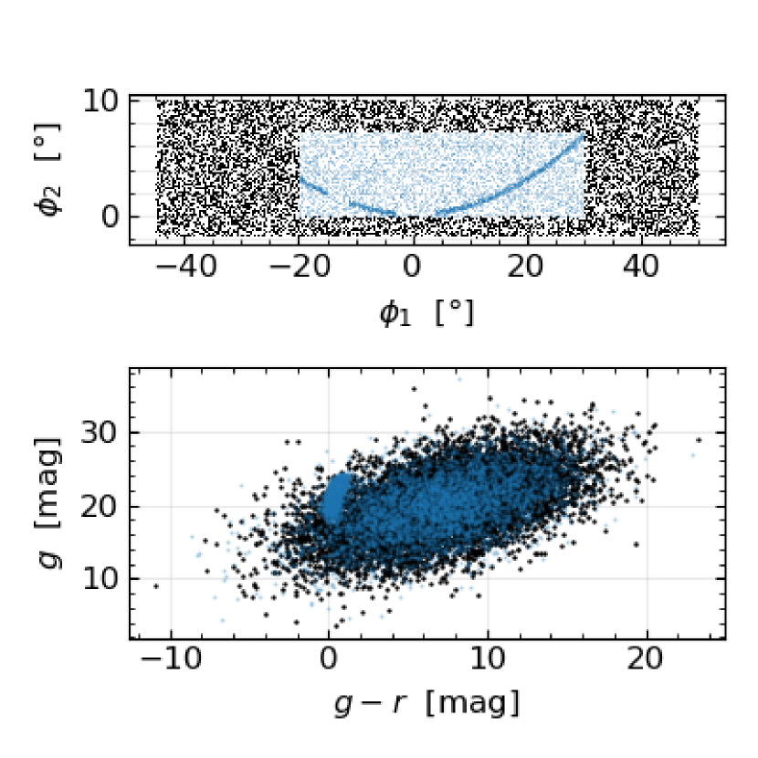
Figure 2: Top panel: Astrometric coordinates ($\phi_{1}$, $\phi_{2}$) for the mock data set. Light blue points are the stream and background within an “on”-stream region. Black points are in the “off”-stream region used to train the background photometric model. Bottom panel: Photometric coordinates for the mock data set. Black points are in the “off”-stream region from the region defined in the astrometric coordinates. Light blue points are the stream and background from the on-stream region. The stream’s isochrone is apparent as an overdensity around (g-r, g)$\ \approx(0,20)$. The background is an arbitrary Gaussian distribution from which the stream must be separated.

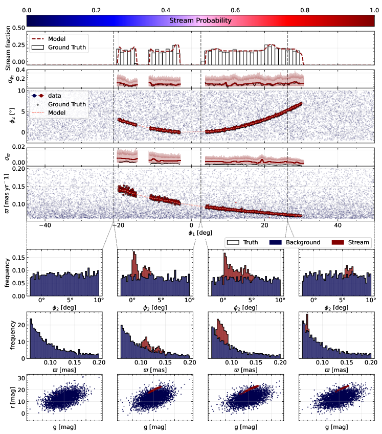
Figure 3: Illustration of the model’s performance in recovering a stream from synthetic observations. The top panel shows the stream mixture coefficient $f(\phi_{1})$ (dashed red line) predicted by the model, overplotted on the true stream fraction (black-outlined histogram). In the middle two rows we also show the $\phi_{2}$ and parallax, $\varpi$, tracks as a function of $\phi_{1}$ and their associated widths (labeled as $\sigma_{\phi_{2}}$ and $\sigma_{\varpi}$, respectively). The true values for these quantities are shown in gray, while our model prediction and uncertainty is show by the dashed red curve and red band, and by the color of the data points (color-coded by membership probability). The model does an excellent job at identifying the ground truth stream stars. In the bottom three rows we demonstrate our ability to separate the stream from the background both astrometrically and photometrically. Histograms are shown for each model component (black for the ground truth, blue for the background, red for the stream), in 4 $\phi_{1}$ ranges across the data set. The height of the histogram is the probability-weighted density for the collection of stars in each bin. There is nearly perfect agreement for the number of stars belonging to each model component as a function of $\phi_{1}$. In the bottom row we show photometric plots for each model component in the same 4 $\phi_{1}$ ranges across the data set. Points are color-coded by stream membership probability.

We select on-stream and off-stream regions using the known $\phi_{1},\phi_{2}$ range of the mock stream. The upper panel of Fig. 2 shows these selections in blue and black, respectively. The lower panel shows the on and off-stream selections in photometric coordinates. In this space it is apparent that the on-stream region has two populations, drawn from the isochrone and from background points included in the simple $\phi_{1},\phi_{2}$ box. In contrast, the off-stream region has only the the background population. We use the off-stream population to train a conditional normalizing flow (see §​​ 2.4) on the magnitudes $g$ and $r$ and conditioned on $\phi_{1}$. The normalizing flow is now a non-parametric distribution characterizing the photometric background, including its variation over $\phi_{1}$. For this mock stream the flexibility of the normalizing flow greatly exceeds necessity: the background is drawn from a $\phi_{1}$-invariant multivariate normal, essentially the base distribution of the normalizing flow. It is therefore no surprise that the trained normalizing flow provides an excellent characterization of the background. We will later see that the flow performs similarly well on complex distributions. Having trained the background photometric model we proceed to build and train the full model.

Per Eq. 6 the stream is an independent addition of both astrometric and photometric models. In astrometrics the stream is a Gaussian track in $\phi_{2}$ and parallax $\varpi$, using the model defined in §​ 2.6.1. We use a 4-layer LTD with overall shape ($\phi_{1}$ input, 4 outputs), where the 4 outputs are $[\mu_{\phi_{2}},\sigma_{\phi_{2}},\mu_{\varpi},\sigma_{\varpi}](\phi_{1})$. The network is small, but sufficiently large to permit 15% dropout and retain robust predictions. The photometric model is a distance modulus-shifted isochrone, using the model outlined in §​ 2.7.1. We use the same isochrone parameters as were used to simulate the stream, including the Grillmair & Smith (2001) mass function. For this mock stream, we demonstrate simultaneous astrometric and photometric modeling, linking the distance modulus and parallax track, as explained in §​ 2.7.2.

The total background model has two pieces, an astrometric and a photometric model. As a pre-training phase the photometric normalizing flow model was fitted to an off-stream selection and is now held fixed. The astrometric model is split in two components, the first is a uniform distribution in $\phi_{2}$, and the second is an exponential distribution for $\varpi$. The uniform distribution does not have any parameters, and thus no neural network. The exponential distribution has only the slope parameter and we use a 3-layer LTD with shape (1, 32, 1) and 15% dropout. Background and stream are combined in a mixture model whose mixture parameters are a 4-layer (1, 64, 1) LTD network. We train the mixture model with an AdamW optimizer with learning rate of $5\times 10^{-3}$ and a scheduler to periodically and temporarily increase the learning rate, encouraging the optimizer towards better minima.

3.3 Trained Density Model

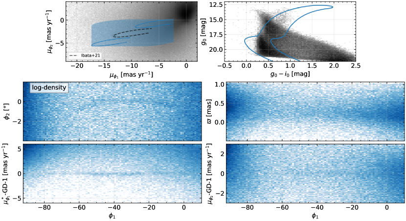
Figure 4: Data selections for GD-1, within the data cube described in §​​ 4.1. Row 1: Proper motion and photometric selections. The proper motion selection is the $[\mu_{\phi_{1}},\mu_{\phi_{2}}](\phi_{1})$ curve from I21 (dashed black line) buffered by $6$ and $3$ mas/yr, respectively (blue curves defining the bottom left and top-right of the shaded rectangular region). Viewed without $\phi_{1}$ we see the $\mu_{\phi_{1}},\mu_{\phi_{2}}$ “phase”-like diagram. The photometric selection is based on a 12 Gyr, [Fe/H] = -1.2 MIST isochrone, buffered by 0.3 mag to select the stream. The data is cut at $G\leq 20$, before applying the isochrone selection. Rows 2 & 3: Applying the combination of astrometric and photometric selections, plotted for astrometric coordinates $\phi_{2},\varpi,\mu_{\phi_{1}},\mu_{\phi_{2}}$. The proper motions are plotted relative to I21. Using a log-density coloring, the stream is identifiable in all phase-space coordinates except $\varpi$ where the errors are significant.

The result of applying our density model to the synthetic data is illustrated in Fig. 3. The top panel shows the weight parameter that controls membership probability as a function of $\phi_{1}$. The dashed curve represents the output of our data-driven model, while the histogram is the ground truth. The second panel shows the stream and background in the $(\phi_{1},\phi_{2})$ plane, and the third panel shows the stream and background in the $(\phi_{1},\varpi)$ plane. Points are color-coded according to their membership probability Eq. 7. The weight parameter clearly shows that the model has captured the two prominent density variations along the stream. There are additional variations, mostly around the edges of the stream, though re-sampling the neural network weights with dropout reveals that these variations represent regions of higher model uncertainty.

We find that the stream is successfully recovered in both astrometric and photometric coordinates, with $>99\%$ of stream stars being recovered with membership probability greater than $80\%$. In the bottom two rows of Fig. 3 we illustrate the synthetic data color-coded by stream membership probability (top) and background membership probability (background) for different $\phi_{1}$ slices. Importantly, the photometric portion of the mixture model successfully identifies the stream in magnitude space, showing a high stream membership probability where the stream is present, and a low probability ($\sim 0$) where the stream is absent. The false positive rate (i.e., stars misidentified as stream members) for this test is found to be $<0.1\%$ (3 stars) when cutting on the 80% membership probability threshold.

4 Results: GD-1

We now apply our method for stream characterization to the stellar stream GD-1, initially discovered by Grillmair & Dionatos (2006a). Previous work has identified several density variations along GD-1 (de Boer et al., 2018), including a bifurcation that can be modeled by an encounter with a dense dark matter subhalo (Bonaca et al., 2019; Webb et al., 2019). Characterizing the detailed density fluctuations of this stream is therefore important for constraining a population of perturbers. We discuss the data selection in §​​ 4.1, model specifics in §​​ 4.2, and the results in §​​ 4.3.

4.1 Data Selection

We utilize data from Gaia DR3 for the astrometric coordinates of each star. To obtain more accurate color information, we cross-match the Gaia field on Pan-STARRS1 (Chambers et al., 2016) using Gaia’s provided Best-neighbors catalog. To limit the field to a region known to contain GD-1 we adopt broad cuts on the cross-matched data. We perform these rough cuts by requiring the data lie within the phase-space cube:

• $\phi_{1}\in[-100,40]\ \rm{deg}$,

• $\phi_{2}\in[-9,5]\ \rm{deg}$,

• $\varpi\in[-10,1]\ \rm{mas}$,

• $G_{\rm BP}\in[-1,3]\ \rm{mag}$

• $g,r\in[0,50]\ \rm{mag}$,

where we use gala’s (Price-Whelan, 2017; Price-Whelan et al., 2020) GD1Koposov10 frame (Koposov et al., 2010) to define $\phi_{1}$, $\phi_{2}$, and associated proper motions. For downloading purposes we split the query into 32 sub-regions in even $\phi_{1}$ increments. Stream-specific coordinates ($\phi_{1},\phi_{2}$) are not included in Gaia. One could embed the coordinate transform in the ADQL (Osuna et al., 2008), or define great-circle arcs in ICRS (Arias et al., 1997). Since only rough cuts are required and since the sub-region boxes are sufficiently small for a reasonable flat-sky approximation we simply translate the ($\phi_{1},\phi_{2}$) boxes to ICRS. We correct the Pan-STARRS1 photometry for dust extinction using the Bayestar19 (Green et al., 2019) models in the dustmaps package (Green, 2018). Bayestar19 is a three-dimensional dust map of the Milky Way for which we use Gaia’s position and parallax distance information. We note that the extinction has very little dependence on the distance past $\approx 8\ \rm{kpc}$. For stars with missing parallax measurements we assume a distance of $8.5\ \rm{kpc}$, a typical distance to the stream, thus increasing potential membership probability. Adopting a slightly lower or higher fiducial distance does not significantly change the results of our analysis. We include the 1$\sigma$ errors as a source of uncertainty in $\boldsymbol{\Sigma}_{n}$, the per-star photometric uncertainty. We also correct the parallax for the zero-point using the gaiadr3-zeropoint package, which implements the findings from Lindegren et al. (2021). The result is a field populated by 8,243,417 stars, from which we would like to identify stream members.

We create data masks for a higher signal-to-noise selection around GD-1. The two mask types, proper motion and photometric, are shown in Fig. 4. For the proper motions we use Ibata et al. (2021) (hereafter I21) as the reference for the known track of the stream. We select all all stars with $\mu_{\phi_{1}}^{*},\mu_{\phi_{2}}$ within 6 mas/yr of the track, as a function of $\phi_{1}$. In Fig. 4 the proper motion data are shown as the difference from the I21 track. In photometric coordinates we define a mask around a $12\ \rm{Gyr}$, [Fe/H] = $-1.2$ isochrone at a distance of $7.8\ \rm{kpc}$. The selection region is a $0.3\ \rm{mag}$ orthogonal buffer around the MIST isochrone (using Speagle et al., 2020), which is illustrated in the 2nd-from-the-top-left plot in Fig. 4. The buffered isochrone selection is wide enough to contain GD-1 over its full distance gradient, including the “typical” distance of 8.5 kpc used in the photometric correction. In addition, to avoid detailed modeling of the completeness as a term in $\mathcal{\pi}_{obs}$ (from Eq. 18) we mask out photometry with $G>20$. With combinations of these masks the stream has much larger signal-to-noise, though is still only a small percent of the total data.

4.2 Model Specification

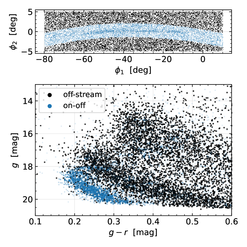
Figure 5: The on and off-stream selection. Top panel: Astrometric coordinates ($\phi_{1}$, $\phi_{2}$). Light blue points are the stream and background within an on-stream region. Black points are in the off-stream region used to train the background photometric model. Note this plot is generated from a reduced field with a tighter proper motion cut to aid in visually identifying the stream. The proper motion cut is $-15<\mu_{\phi_{1}}^{*}<-10$, $-4.5<\mu_{\phi_{2}}<-2$ [mas/yr]. Bottom panel: CMD of the astrometric selection above. The stream’s isochrone is apparent as an overdensity.

The modeling framework, detailed in section §​ 2, is modular, allowing many model components to be combined, nested, added to the mixture, and linked via priors. The model we require for GD-1 is similar to the model built for the mock stream in §​​ 3.2, but has additional components for GD-1’s spur. In this section we will discuss how the total model is built, noting similarities to the example mocks-stream model.

All full stream models necessarily include a background model, which we model in both astrometric and photometric spaces. The photometric background is too complex to capture with simple analytic distributions. Instead, we train a normalizing flow on the magnitudes $g,r$, conditioned on $\phi_{1}$. We refer readers to §​​ 2.4 for discussion of the photometric distribution and how a normalizing flow can characterize this complex distribution, including its variation over $\phi_{1}$. The flow’s flexibility, while necessary in this context, also poses a problem: the flow captures the stream as easily as the background. Consequently we select on-stream and off-stream regions using the known $\phi_{1},\phi_{2}$ range of the stream, as shown in the upper panel of Fig. 5. In the lower panel we plotted this selection in photometric coordinates, where an isochrone is apparent in the on-stream selection. The normalizing flow is trained on the off-stream selection, and will be fixed (not trainable, nor contribute to the gradient) when incorporated into the larger model.

Unlike for the photometry, the astrometric background could be (mostly) fit with simple analytic distributions. This is true if the selected field is large enough – the distribution in each coordinate is approximately a skew-normal or a similarly tailed exponential-type function. However by defining a higher signal-to-noise field around the Ibata et al. (2021) stream track in $\mu_{\phi_{1}}^{*},\mu_{\phi_{2}}$, the background in these coordinates is no longer well described by an exponential distribution. Similarly, for much of the extent of GD1’s field the parallax is well modeled by a truncated skew-normal distribution, $\varpi\sim\rm{TruncSkew}\mathcal{N}(\mu,\Sigma;a,b)$, however for $\phi_{1}\in[-100,-60]$ this does not hold. Rather than splitting the model at a somewhat arbitrary $\phi_{1}$ or interpolating between two distributions we instead fit the astrometry with a $\phi_{1}$-conditioned normalizing flow. The background model is characterized by:

• $\phi_{2},\sim\rm{TruncExp}(\lambda;a,b)$: a truncated exponential distribution (see §​​ A.2). The distribution has 1 slope parameter.

• $\mu_{\phi_{1}}^{*},\mu_{\phi_{2}},\varpi\sim q_{\rm flow}$: a 3 argument , one context feature ($\phi_{1}$) normalizing flow trained on an off-stream selection (see Fig. 5 for that selection). Though discussed in the context of a photometric background, §​​ 2.4 details how these flows are constructed and trained.

We model the main stream of GD-1 similarly to the mock stream – as an independent addition of both astrometric and photometric models. The astrometric model for the stream is a 5-dimensional Gaussian in a Gaussian track in $\phi_{2},\varpi,\mu_{\phi_{1}},\mu_{\phi_{2}},\varpi$, using the model defined in §​ 2.6.1. The parameter network’s 10 outputs are $\boldsymbol{\theta}=[\mu_{\phi_{2}},\sigma_{\phi_{2}},\mu_{\varpi},\sigma_{\varpi},\mu_{\mu_{\phi_{1}}^{*}},\sigma_{\mu_{\phi_{1}}^{*}},\mu_{\mu_{\phi_{2}}},\sigma_{\mu_{\phi_{2}}},\mu_{\varpi},\sigma_{\varpi}](\phi_{1})$. In testing the network is sufficiently large to permit 15% dropout and retain robust predictions.

The stream’s photometric model is a distance modulus-shifted isochrone, using the model from §​ 2.7.1. We use a $12\ \rm{Gyr}$, [Fe/H]$=-1.2$ MIST isochrone with no assumed intrinsic dispersion. GD-1’s true spectroscopic metallicity is [Fe/H]$\lesssim-2$, but there is enough degeneracy in age and metallicity that the chosen isochrone empirically matches the CMD locus and is useful in this modeling context. Using the method described in §​ 2.7.2 the distance modulus track is set by the parallax track in the astrometric model. Thus the on-stream photometric model has no independent parameters and consequently no neural network.

Table 1: Stream Track Regions Prior: This table includes all the region priors used to guide the model towards the known stream track. The model will converge to the region ${}_{\rm minimum}^{\rm maximum}$. See §​ 2.8.2 for details.

component	$\phi_{1}\,[\rm{\degree}]$	$\phi_{2}\,[\rm{\degree}]$	$\mu_{\phi_{1}}\,[\frac{\rm{mas}}{\rm{yr}}]$	$\mu\,[\rm{mag}]$	$(\simeq\varpi\,[\text{mas}])$
stream	-90.0	${\color[rgb]{.5,.5,.5}\big{(}}_{-5.28}^{-1.78}{\color[rgb]{.5,.5,.5}\big{)}}$
stream	-80.0	${\color[rgb]{.5,.5,.5}\big{(}}_{-3.93}^{-0.43}{\color[rgb]{.5,.5,.5}\big{)}}$
stream	-70.0	${\color[rgb]{.5,.5,.5}\big{(}}_{-2.89}^{\phantom{+}0.61}{\color[rgb]{.5,.5,.5}\big{)}}$	${\color[rgb]{.5,.5,.5}\big{(}}_{-12.20}^{-10.20}{\color[rgb]{.5,.5,.5}\big{)}}$	${\color[rgb]{.5,.5,.5}\big{(}}_{14.20}^{14.80}{\color[rgb]{.5,.5,.5}\big{)}}$	${\color[rgb]{.5,.5,.5}\big{(}}_{0.11}^{0.15}{\color[rgb]{.5,.5,.5}\big{)}}$
stream	-60.0	${\color[rgb]{.5,.5,.5}\big{(}}_{-2.13}^{\phantom{+}1.37}{\color[rgb]{.5,.5,.5}\big{)}}$	${\color[rgb]{.5,.5,.5}\big{(}}_{-13.30}^{-11.70}{\color[rgb]{.5,.5,.5}\big{)}}$
stream	-50.0	${\color[rgb]{.5,.5,.5}\big{(}}_{-1.66}^{\phantom{+}1.84}{\color[rgb]{.5,.5,.5}\big{)}}$	${\color[rgb]{.5,.5,.5}\big{(}}_{-14.05}^{-12.55}{\color[rgb]{.5,.5,.5}\big{)}}$
stream	-40.0	${\color[rgb]{.5,.5,.5}\big{(}}_{-1.46}^{\phantom{+}2.04}{\color[rgb]{.5,.5,.5}\big{)}}$	${\color[rgb]{.5,.5,.5}\big{(}}_{-14.05}^{-12.55}{\color[rgb]{.5,.5,.5}\big{)}}$	${\color[rgb]{.5,.5,.5}\big{(}}_{14.10}^{14.70}{\color[rgb]{.5,.5,.5}\big{)}}$	${\color[rgb]{.5,.5,.5}\big{(}}_{0.11}^{0.15}{\color[rgb]{.5,.5,.5}\big{)}}$
spur	-35.0	${\color[rgb]{.5,.5,.5}\big{(}}_{0.45}^{2.15}{\color[rgb]{.5,.5,.5}\big{)}}$	${\color[rgb]{.5,.5,.5}\big{(}}_{-14.95}^{-10.95}{\color[rgb]{.5,.5,.5}\big{)}}$
stream	-30.0	${\color[rgb]{.5,.5,.5}\big{(}}_{-1.51}^{\phantom{+}1.99}{\color[rgb]{.5,.5,.5}\big{)}}$	${\color[rgb]{.5,.5,.5}\big{(}}_{-13.35}^{-11.85}{\color[rgb]{.5,.5,.5}\big{)}}$
spur	-30.0	${\color[rgb]{.5,.5,.5}\big{(}}_{0.45}^{2.15}{\color[rgb]{.5,.5,.5}\big{)}}$	${\color[rgb]{.5,.5,.5}\big{(}}_{-14.60}^{-10.60}{\color[rgb]{.5,.5,.5}\big{)}}$
stream	-20.0	${\color[rgb]{.5,.5,.5}\big{(}}_{-1.80}^{\phantom{+}1.70}{\color[rgb]{.5,.5,.5}\big{)}}$
spur	-20.0	${\color[rgb]{.5,.5,.5}\big{(}}_{0.65}^{2.35}{\color[rgb]{.5,.5,.5}\big{)}}$	${\color[rgb]{.5,.5,.5}\big{(}}_{-13.50}^{\phantom{+}-9.50}{\color[rgb]{.5,.5,.5}\big{)}}$
stream	-10.0	${\color[rgb]{.5,.5,.5}\big{(}}_{-2.32}^{\phantom{+}1.18}{\color[rgb]{.5,.5,.5}\big{)}}$	${\color[rgb]{.5,.5,.5}\big{(}}_{-11.75}^{\phantom{+}-8.25}{\color[rgb]{.5,.5,.5}\big{)}}$
stream	0.0	${\color[rgb]{.5,.5,.5}\big{(}}_{-3.05}^{\phantom{+}0.45}{\color[rgb]{.5,.5,.5}\big{)}}$		${\color[rgb]{.5,.5,.5}\big{(}}_{14.70}^{15.30}{\color[rgb]{.5,.5,.5}\big{)}}$	${\color[rgb]{.5,.5,.5}\big{(}}_{0.08}^{0.12}{\color[rgb]{.5,.5,.5}\big{)}}$
stream	5.0		${\color[rgb]{.5,.5,.5}\big{(}}_{-9.15}^{-5.65}{\color[rgb]{.5,.5,.5}\big{)}}$
stream	10.0	${\color[rgb]{.5,.5,.5}\big{(}}_{-3.97}^{-0.47}{\color[rgb]{.5,.5,.5}\big{)}}$

We model the spur of GD-1 as a separate component to the main stream. The spur has an identical model as the stream: a 5-D astrometric Gaussian and isochrone in the photometry. Owing to their common origin, we impose the prior that the spur and stream share the same isochrone. The parallax is also shared, motivated by initial findings, and that there were too few stars to robustly detect any deviations.

Table 2: Subset of GD-1 Membership Table.
This table includes a selection of candidate member stars for the GD-1 stream, based on the membership likelihoods. For each star we include the Gaia DR3 source ID and astrometric solution, the Pan-STARRS1 photometry, and the membership likelihoods for the stream, spur, and background. The likelihoods are computed using the trained model described in §​​ 4.3 and we include a quality flag ${\rm dim}(\boldsymbol{x})$, indicating the number of features used by the model. For most stars all features are measured. We use dropout regularization to estimate the uncertainty in the likelihoods, and report the 5% and 95% quantiles of the distribution, as well as the dropout-disabled maximum-likelihood estimate (MLE) of the likelihood.
We include as interesting cases:
$\phantom{+}\ast$  1 star with the highest MLE for the stream,
$\phantom{+}\ast$  5 stars with high stream MLE ($\mathcal{L}^{(S)}_{\rm MLE}>0.9$),
$\phantom{+}\ast$  4 stars with low stream MLE, but whose 95% likelihood is high ($\mathcal{L}^{(S)}_{\rm MLE}<0.75,\mathcal{L}^{(S)}_{\rm 95\%}>0.8$),
$\phantom{+}\ast$  1 star with the maximum MLE for the spur,
$\phantom{+}\ast$  1 star with high spur MLE and low stream MLE ($\mathcal{L}^{(spur)}_{\rm MLE}>0.9,\mathcal{L}^{(S)}_{\rm MLE}<0.75$),
For convenience we round the likelihoods to 2 decimal places, and only show the value and uncertainty when it is non-zero.
The full table, including source ids, is available online.

Gaia						PS-1			Membership Likelihood (${\rm MLE}_{\phantom{0}5\%}^{95\%}$)
source_id	$\alpha$ [∘]	$\delta$ [∘]	$\mu_{\alpha}^{*}$ [$\frac{\rm{mas}}{\rm{yr}}$]	$\mu_{\delta}$ [$\frac{\rm{mas}}{\rm{yr}}$]	$\varpi$ [mas]	g [mag]	r [mag]	${\rm dim}(\boldsymbol{x})$	$\mathcal{L}_{\rm stream}$	$\mathcal{L}_{\rm spur}$	$\mathcal{L}_{\rm background}$
—	207.32	58.53	$-7.71\pm 0.01$	$-2.85\pm 0.01$	$0.08\pm 0.01$	$14.14\pm 0.01$	$13.37\pm nan$	7	$1.00$	—	—
—	138.13	20.99	$-3.78\pm 0.27$	$-12.66\pm 0.20$	$0.22\pm 0.28$	$19.15\pm 0.02$	$18.91\pm 0.02$	7	$0.99_{-0.04}^{+0.00}$	—	$0.01_{-0.00}^{+0.04}$
—	166.42	49.40	$-7.08\pm 0.06$	$-9.72\pm 0.08$	$0.04\pm 0.09$	$17.53\pm 0.00$	$17.14\pm 0.00$	7	$0.99_{-0.10}^{+0.01}$	—	$0.01_{-0.01}^{+0.10}$
—	159.37	45.40	$-6.94\pm 0.22$	$-11.34\pm 0.22$	$0.43\pm 0.27$	$19.76\pm 0.02$	$19.48\pm 0.01$	7	$0.96_{-0.42}^{+0.03}$	$0.00_{-0.00}^{+0.03}$	$0.04_{-0.02}^{+0.41}$
—	146.05	32.95	$-5.13\pm 0.25$	$-12.72\pm 0.18$	$0.36\pm 0.23$	$19.02\pm 0.02$	$18.81\pm 0.02$	7	$0.95_{-0.11}^{+0.02}$	$0.03_{-0.02}^{+0.08}$	$0.01_{-0.00}^{+0.04}$
—	145.70	32.85	$-5.14\pm 0.38$	$-12.48\pm 0.26$	$0.18\pm 0.40$	$19.74\pm 0.02$	$19.47\pm 0.02$	7	$0.95_{-0.13}^{+0.02}$	$0.04_{-0.02}^{+0.13}$	$0.01_{-0.01}^{+0.01}$
—	190.27	57.04	$-7.52\pm 0.43$	$-5.50\pm 0.40$	$0.16\pm 0.38$	—	—	5	$0.74_{-0.61}^{+0.12}$	—	$0.26_{-0.12}^{+0.61}$
—	135.37	16.22	$-2.82\pm 0.79$	$-12.77\pm 0.52$	$0.72\pm 0.88$	—	—	5	$0.72_{-0.43}^{+0.13}$	—	$0.28_{-0.13}^{+0.43}$
—	164.08	47.92	$-8.06\pm 0.16$	$-10.93\pm 0.20$	$0.19\pm 0.21$	$19.28\pm 0.01$	$19.07\pm 0.01$	7	$0.69_{-0.66}^{+0.16}$	—	$0.31_{-0.16}^{+0.66}$
—	146.51	34.16	$-5.01\pm 0.25$	$-13.06\pm 0.22$	$0.33\pm 0.23$	$19.07\pm 0.01$	$18.85\pm 0.01$	7	$0.63_{-0.30}^{+0.18}$	$0.30_{-0.18}^{+0.23}$	$0.08_{-0.02}^{+0.16}$
—	156.99	44.64	$-6.41\pm 0.31$	$-11.47\pm 0.40$	$0.74\pm 0.40$	$19.86\pm 0.06$	$19.63\pm 0.05$	7	—	$0.99_{-0.01}^{+0.00}$	$0.01_{-0.00}^{+0.01}$
—	149.88	38.71	$-5.87\pm 0.25$	$-12.42\pm 0.20$	$0.00\pm 0.25$	$19.34\pm 0.02$	$19.12\pm 0.01$	7	$0.00_{-0.00}^{+0.01}$	$0.96_{-0.12}^{+0.01}$	$0.04_{-0.01}^{+0.12}$

The parameter phase-space is large and a random initialization will take significant time to converge towards the stream track. This initial training is unnecessary as the rough stream track is known a priori. To guide the astrometric model towards the known GD-1, we set down guides (see §​ 2.8.2) along GD-1’s main track and on the spur. We set the width of these guides to large values, so that their influence on the model is not dominant. Indeed, we find that the value of the guides is to help reduce training time, since otherwise it will take the flexible density model much longer to converge to the actual stream. We include all the track regions in Table 1.

All the component models are tied together into a mixture model. The singular weight parameter network is a LTD network with 15% dropout. The stream weights are in the range $\ln f\in[-10,0]$, while the spur weights are $\ln f\in[-10,0]$ and set to 0 for $\phi_{1}<-45,-15<\phi_{1}$. By Eq. 3 the background brings the cumulative weight to one, normalizing the mixture.

4.3 Trained Density Model

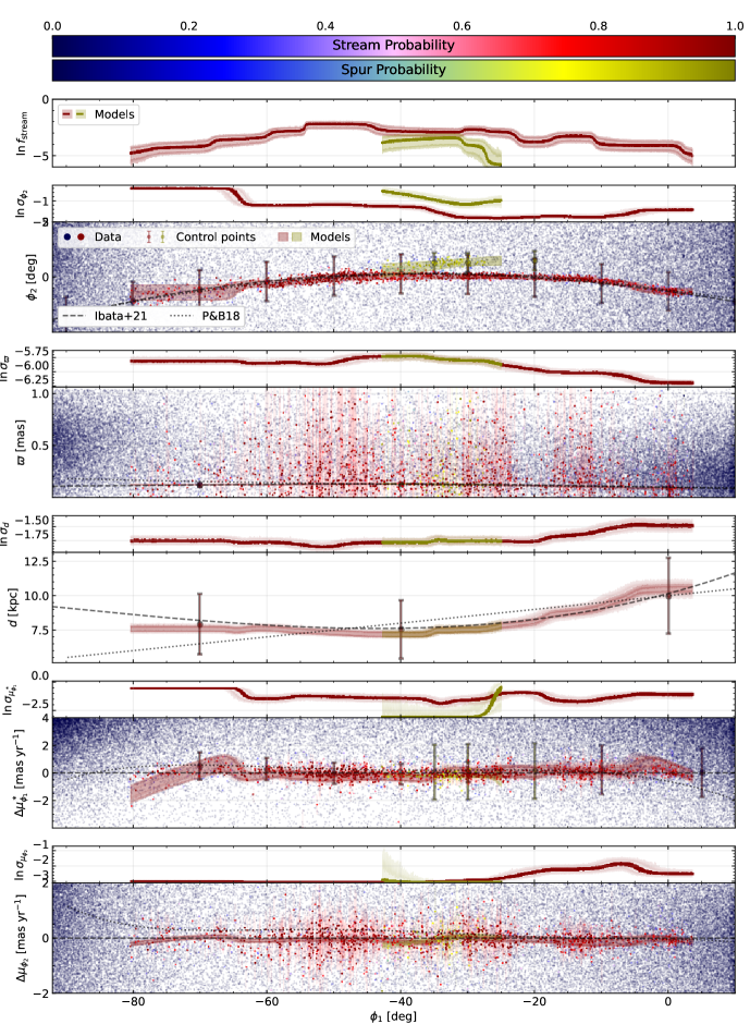
Figure 6: The model for GD-1, including both a thin-stream and spur component. For comparison we include the tracks from Price-Whelan & Bonaca (2018) and Ibata et al. (2021). Note how the model largely agrees with the latter track in all astrometric dimensions. Panel 1: The stream mixture coefficients $f(\phi_{1})$ predicted by the model, colored by the stream and spur membership likelihood. Panel 2: $\phi_{2}(\phi_{1})$ over the full range of $\phi_{1}$. The data color and transparency are set by the model’s 50th-percentile stream and spur probability. We include the error bars for stars with $>75\%$ membership probability. The predicted 50th-percentile track $\pm$ width is over-plotted (red band), along with the 90% confidence region (broader red band). The 5th to 95th percentile variation in the width is shown in the adjoining top plot. Panel 3 & 4: $\varpi(\phi_{1})$ and $d(\phi_{1})$ over the full range of $\phi_{1}$. The $\varpi$ is tied to the photometry – see Fig. 7. Panel 5 & 6: The proper motions $\Delta\mu_{\phi_{1}^{*}},\Delta\mu_{\phi_{2}}$ shown relative to the galstreams track (black dashed line). The model convolves observational errors with the stream width, but the large fractional errors make the determination difficult.

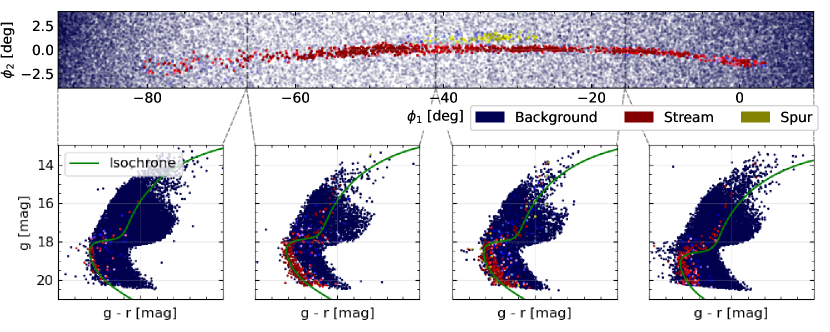
Figure 7: Photometric coordinate $(g,r)$ plots for each model component in 4 $\phi_{1}$ ranges across the data set. Over-plotted is the model isochrone, shifted to the mean distance of the track within the selected $\phi_{1}$ range. Importantly this means we do not expect the mean isochrone to exactly match the distribution of points. See Fig. 6 for the match of the distance gradient to the data and prior literature results.

In this section we present results from our model applied to real Gaia and Pan-STARRS data of GD-1. We visualize the performance of our model in identifying stream stars in Fig. 6, and illustrate our photometric fit in Fig. 7. In Table 2 we provide a selection of GD-1 member stars. The full catalog is available online at zenodo:10211410. Lastly, Fig. 8 is a membership probability-weighted density heatmap of the GD-1 stream derived from our fit.

In Fig. 6, the top panels shows the fraction of stars belonging to the stream (red) and spur (yellow) as a function of $\phi_{1}$. The second panel illustrates the stream in $\phi_{1}$, $\phi_{2}$ coordinates, color-coded by the membership probability for the stream and spur components (derived from Eq. 7). The following rows represent the other astrometric dimensions for the stream and spur components, with the distance track obtained through our photometric model (visualized in Fig. 7 and discussed below). The red and yellow bands represent model predictions for the main stream and spur, respectively. The points with thick error bars represent control points (discussed in §​​ 4.2) for the stream and spur components, which are priors on the location of the stream and spur components across the astrometric dimensions. The control points in the parallax panel represent the reliable parallax and distance modulus estimates from de Boer et al. (2020). The actual data points are color-coded by the maximum membership probability of belonging to any of the three model components (i.e., maximum of the main stream, spur, or background components). For stars with membership probability greater than $75\%$, we also plot their astrometric errorbars from Gaia as the thin red lines.

Because the neural networks are trained with dropout, we can estimate the modeling uncertainty in our fits to each stream with a Monte Carlo procedure (Gal & Ghahramani, 2015). Namely, by incorporating dropout during both neural network training and inference, the distribution of model outputs represents the posterior predictive distribution, marginalized over the neural network parameters. An estimate of this distribution is shown in the weight parameter of Fig. 6, represented as the red (main stream) and yellow (spur) bands. For the astrometric dimensions, our model predicts a mean track, and a standard deviation. Error bands are estimated by incorporating dropout with a rate of 15%. Each of the panels in Fig. 6 shows the track mean and width, calculated from the 50th percentile of the posterior predictive distribution for both quantities. Plotted behind that is the 90% credible region of the track mean. We note that the credible region of the mean alone is generally larger than that of the $\mu\pm\sigma$ 50th-percentile ridge. This highlights the importance of exploring the full posterior of parameters, not only a Maximum Likelihood Estimation (MLE) or posterior ridge-line.

Our model finds $730$ stars that belong to the main stream component with membership probability greater than $80\%$ at the $50$th percentile in the membership posterior distribution. For the spur component, there are $37$ stars with the same membership probability threshold at the same percentile of the posterior distribution. A tabulation of the astrometry, photometry, and membership posterior distribution for each star is included in Table 2. The full table may be found on the paper’s GitHub repository. Table 2 gives the MLE prediction, but also samples the 5th-95th percentile of the posterior distribution of the likelihood using the dropout method. The variation in the 90% credible region in the track means there can be significant variation in a star’s estimated membership probability.

The extent of the main stream in $\phi_{1}$ is roughly $80~{}\rm{deg}$, and the angular extent of the spur is roughly $15~{}\rm{deg}$. The distance track (bottom panel) places the stream in the range of $6-10~{}\rm{kpc}$, with an upwards concavity as a function of $\phi_{1}$. This result is consistent with other works, which find a similar distance to GD-1 using other techniques (de Boer et al., 2020; Ibata et al., 2021). Importantly, our distance estimate is not hard-coded to fall in this range: we allow for the stream track to fall anywhere within $[4,40]~{}\rm{kpc}$, with a broad prior around previous literature estimates. The similarity of our inferred distance track compared to other works indicates that our photometric model is performing satisfactorily.

We also recover the well-known underdensity gaps along the stream around $\phi_{1}\approx-40,-20\ \rm{and}-5~{}\rm{deg}$ (seen best in Fig. 8). The $-20\degree$ feature was first reported by Carlberg & Grillmair (2013), and is one location hypothesized for the dissolved stream progenitor. Webb & Bovy (2019) suggests the $-40\degree$ gap might be the progenitor location. The recovery of this density fluctuation from a joint model in astrometric and photometric coordinates developed here argues that the feature is indeed intrinsic to the stream and not an artifact of the data.

The spur is a distinct component of our model, independent in its weight and all astrometric dimensions except $\varpi$ which is shared with the GD-1 main stream through the photometric model. The model finds a non-negligible spur feature, with a peak fractional weight approaching the thin stream. As corroboration, the proper motion of the spur closely agrees with the thin stream. The alignment of these dimensions is not hard-coded in our model. The width of the spur in proper motion is very thin, thinner even than the stream. However with the large observational errors and low number density of the spur it is difficult to attribute this to a physical difference between the two systems. In contrast, the small errors in $\phi_{2}$ indicate the spur’s width diverges from the thin stream at $\phi_{1}>-35\ \rm{deg}$, whereas the width is similar at lower $\phi_{1}$. There are numerous mechanisms by which a stream’s width may vary (e.g. epicyclic effects as in Ibata et al., 2020), so differences between the spur and stream are both notable and expected.

GD-1 has other observed tidal features, namely the “blob” (Price-Whelan & Bonaca, 2018), which is a very diffuse component enclosing the thin stream. When fitting our model to GD-1 with a more stringent proper motion cut, we are able to recover the blob. In a more crowded field, the stream makes up only a few percent of the total number of stream stars, so diffuse features like the blob are not separated from the background. We could, perhaps, guide the model towards the blob by adding an additional mixture distribution that is specialized to diffuse components around the thin stream. Because the aim of the current paper is to introduce and demonstrate our method, we defer a more detailed fit of the diffuse extra-tidal structure of Milky Way streams to future work.

We note that the model-predicted track does not always closely align with the predicted member stars or our notion of a slowly-evolving stream. This misalignment is most evident in $\mu_{\phi_{1}^{*}}$, where the track has a sharp turn up at $\phi_{1}\sim-65\ \rm{deg}$ and then flattens out. There are a number of contributing factors. First, the observational uncertainties are large enough that this flattening is consistent with the data. Second, we do not enforce the stream track to be smooth with $\phi_{1}$ – our fits are dictated by the data. Last, examining 2D slices when fitting in high dimensional spaces can be misleading (Aggarwal et al., 2002). Unsurprisingly, the raw membership probabilities for each model component provide a more accurate representation of the stream’s 6d phase-space distribution than any phase-space slice could, as may be seen in Fig. 8. We discuss the smoothed stream model determined solely by membership probabilities at the end of this section.

We highlight the performance of our photometric model in Fig. 7. In this figure, we color-code each star by its membership probability (top row; same as Fig. 6), and in the bottom row we visualize the performance of our photometric model in bands of $\phi_{1}$. Our model isochrone, which shifts vertically due to our distance modulus estimate, is shown in green (we plot the mean-distance isochrone in each $\phi_{1}$ band). Because our model preforms a joint fit in photometry and astrometry, the most probable stream members do not need to fall exactly along the isochrone. Still, the likely stream members are overwhelmingly distributed as might be expected from a single-stellar population. Even the more diffuse tails of the stream can be seen in the CMD distribution, where they still roughly follow a single-stellar population.

With membership probabilities for each component of the stream estimated from both astrometry and photometry, it is possible to quickly construct a custom representation of the stream’s phase-space density. We illustrate this in Fig. 8, which shows a Gaussian kernel density estimate (KDE) of bandwidth $0.1\ \rm{deg}$ (or mas/yr) fit to the model. The primary overdensities at $\phi_{1}=(-50,-30,-10)\ \rm{deg}$ are all visible in $\phi_{2}$. The gap at $20\ \rm{deg}$ is prominent in all features, but the gap at $-40$ is less visible in proper motions, since the spur shares the stream’s proper motions and thus contributes to the density in those coordinates. This highlights the importance of constructing a multidimensional smooth density model of streams.

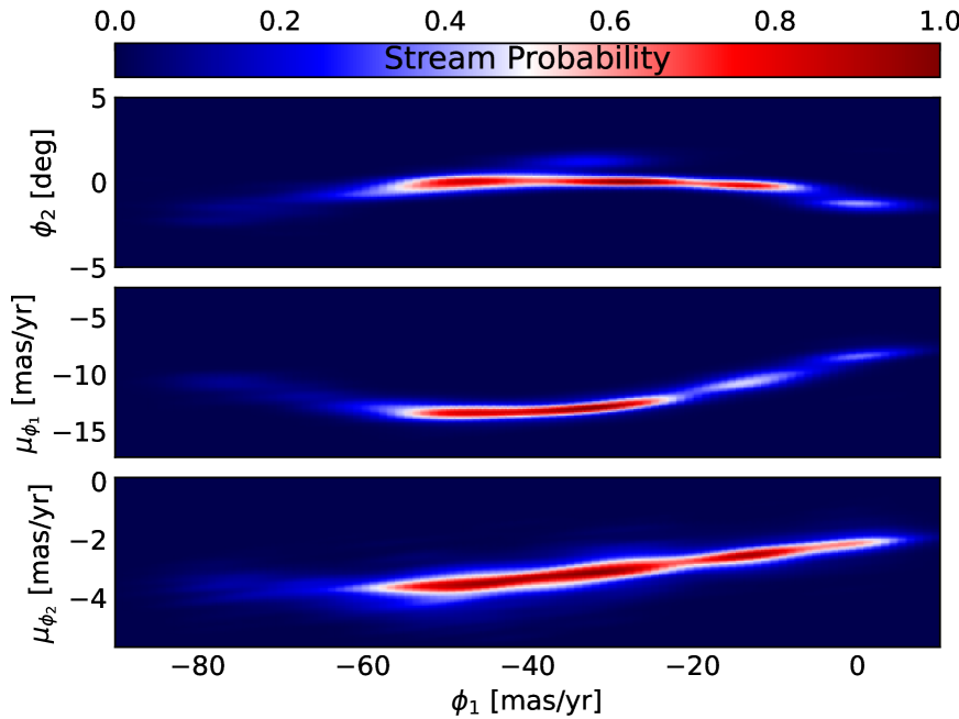
Figure 8: Smoothed KDE model of GD-1’s member stars, weighted by their membership probability. The KDE has a bandwidth of $0.1\ \rm{deg}$ (or mas/yr). In $\phi_{2}$ the spur is clearly visible in the KDE. The gaps at $-20\degree$ are prominent in both $\phi_{2}$ and $\mu_{\phi_{1}}$. The gap at $-40\degree$ is most prominent in $\phi_{2}$.

5 Results: Palomar 5

We now apply the method to the stellar stream Palomar 5. Historically lengths of the stream have been found with matched filter photometric techniques, like with the discovery in Odenkirchen et al. (2001). Post-Gaia the stream was also observed by filtering kinematically (e.g., Starkman et al., 2019; Ibata et al., 2021). However at $\sim 20\ \rm{kpc}$, the Pal 5 main sequence is not observed by Gaia, making a high signal-to-noise astrometric detection challenging. We discuss the data selection in §​​ 5.1, model specifics in §​​ 5.2, and the results in §​​ 5.3.

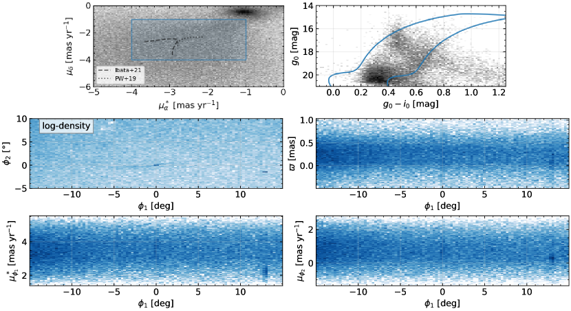
Figure 9: Data selections for Pal 5, within the data cube described in §​​ 5.1. Row 1: Proper motion and photometric selections. Pal 5 is apparent in the proper motions as a small overdensity. The photometric selection is based on a 12 Gyr, [Fe/H] = -1.2 MIST isochrone, buffered by 0.3 dex. The photometry is also cut to Gaia’s $G\leq 20$ mag, before applying the isochrone selection. Rows 2 & 3: Applying the combination of astrometric and photometric selections, plotted for astrometric coordinates $\phi_{2},\varpi,\mu_{\phi_{1}},\mu_{\phi_{2}}$. The stream is an identifiable overdensity in only $\phi_{2}$ and errors dominate all other coordinates.

5.1 Data Selection

We construct a Gaia DR3 - Pan-STARRS1 crossmatched field very similarly to the procedure outlined in §​​ 4.1 for GD-1. To limit the field to a region containing Pal 5 we adopt broad cuts on the data by requiring the data lie within the phase-space cube:

• $\phi_{1}\in[-20,20]\ \rm{deg}$,

• $\phi_{2}\in[-5,10]\ \rm{deg}$,

• $\varpi\in[-10,1]\ \rm{mas}$,

• $\rm{G-R}\in[-0.5,1.2]\ \rm{mag}$

• $g,r\in[0,30]\ \rm{mag}$,

where we use gala’s Pal5PriceWhelan18 frame (Price-Whelan et al., 2019) to define $\phi_{1}$, $\phi_{2}$, and associated proper motions. Using the Bayestar19 maps we correct the Pan-STARRS1 photometry for dust extinction. For stars without distance information we assume a distance of $20\ \rm{kpc}$, a typical distance to the stream (Harris, 1996; Odenkirchen et al., 2003; Grillmair & Dionatos, 2006b; Ibata et al., 2016; Price-Whelan et al., 2019) and thus increasing the probability of the star being considered a member. The 1$\sigma$ dust correction errors are included by quadrature in $\boldsymbol{\Sigma}_{n}$, the per-star photometric uncertainty. We also correct the parallax for the Gaia zero-point as in §​​ 4.1. The result is a field populated by 5,022,757 stars, from which we would like to identify stream members.

Within the broad selection cuts, we create more specific data masks. In particular we mask concentrated over-densities, like the globular cluster M5, that are not associated with Pal 5. In Fig. 9 we show the proper motion and photometric masks, with M5 already filtered out. The proper motion mask extends from $\mu_{\phi_{1}}$ and $\mu_{\phi_{2}}\in(-4,-1)$ [mas/yr]. The photometric mask is defined by a $0.15\ \rm{mag}$ buffer around a $[\rm{Fe}/{H}]=-1.3$, $11.5\ \rm{Gyr}$ isochrone. It is the shape of the isochrone which is important, not the physical reality of the metallicity nor age, discussed in further detail in §​ 2.7.1. In addition, to avoid detailed modeling of the completeness as a term in $\mathcal{\pi}_{obs}$ (from Eq. 18) we mask out photometry with $G>20$. With combinations of these masks the stream has much larger signal-to-noise, though is still only a small fraction of the total data.

The reduced dataset, with all specific masks applied, is included below the data mask plots in Fig. 9. In $\phi_{2}$, $\mu_{\phi_{1}}^{*}$, and $\mu_{\phi_{2}}$ the Pal 5 progenitor is clearly visible. Only in $\phi_{2}$ is the stream visible, and then only for a few degrees around the progenitor. The distance of Pal 5 means most $\varpi$ measurements have $\sim 100\%$ errors, so neither the stream nor even the progenitor are evident.

5.2 Model Specification

In this section we discuss how the total Pal 5 model is built, using the modular modeling framework from §​ 2. We model the stream of Pal 5 as a single Gaussian component conditioned on $\phi_{1}$. As a function of $\phi_{1}$, the astrometric stream density is a 3-dimensional Gaussian in $\phi_{2},\mu_{\phi_{1}},\mu_{\phi_{2}}$, using the model defined in §​ 2.6.1. The parameter network is a 5-layer LTD where the 6 outputs are $\boldsymbol{\theta}=[\mu_{\phi_{2}},\sigma_{\phi_{2}},\mu_{\mu_{\phi_{1}}^{*}},\sigma_{\mu_{\phi_{1}}^{*}},\mu_{\mu_{\phi_{2}}},\sigma_{\mu_{\phi_{2}}}](\phi_{1})$. In testing, the network is sufficiently large to permit 15% dropout and retain robust predictions. At $\sim 20\ \rm{kpc}$ any Gaia-crossmatched data is not photometrically deep enough to contain the main sequence nor its turn off. Thus we do not model the stream photometrically. We only use photometric cuts to remove some background. Similarly, we do not include the parallax as the errors are too large for the parallax to contribute to the model.

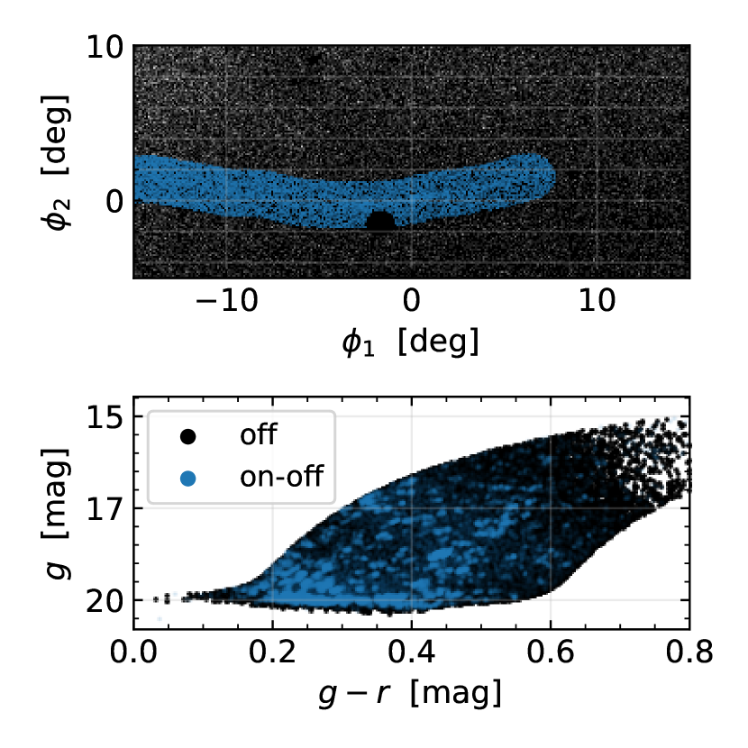
Figure 10: Top panel: Astrometric coordinates ($\phi_{1}$, $\phi_{2}$). Light blue points are the stream and background within an “on”-stream region. Black points are in the “off”-stream region used to train the background photometric model. The M5 cluster is masked as a black circle cutting into the on-stream selection at $\phi_{1}\sim-1\degree$. Bottom panel: CMD plot of the astrometric selection above. The stream’s isochrone is somewhat apparent, but the background contamination is large.

To avoid a large convergence time, we use as a prior the known stream track, in this case galstream’s (Mateu, 2022) implementation of Pal 5 from Ibata et al. (2021). From the track, we set down guides (see §​ 2.8.2) regularly spaced in $\phi_{1}$. We include all the guides in Table 3. We don’t place guides in the other coordinates, except at the location of the progenitor, because the stream is not visible and the models disagree on the proper motions (see Fig. 9, top left plot). The progenitor is an exception, both visible kinematically and also extremely well measured (Vasiliev & Baumgardt, 2021), and we place a tight kinematic prior on the stream track at the location of the progenitor. The guide priors are visible in Fig. 11.

Table 3: Stream Track Regions Priors for Pal 5: This table includes all the region priors used to guide the model towards the known stream track. The model will converge to the region ${}_{\rm minimum}^{\rm maximum}$. The regions are determined by the stream track from galstreams (Mateu, 2022), with a width significantly larger than the stream width. In the kinematics only the progenitor is used to guide the model.

$\phi_{1}\,[\rm{\degree}]$	$\phi_{2}\,[\rm{\degree}]$	$\mu_{\phi_{1}}\,[\frac{\rm{mas}}{\rm{yr}}]$	$\mu_{\phi_{2}}\,[\frac{\rm{mas}}{\rm{yr}}]$
-12.71	${\color[rgb]{.5,.5,.5}\big{(}}_{-0.08}^{\phantom{+}1.92}{\color[rgb]{.5,.5,.5}\big{)}}$
-10.30	${\color[rgb]{.5,.5,.5}\big{(}}_{-0.44}^{\phantom{+}1.56}{\color[rgb]{.5,.5,.5}\big{)}}$
-7.89	${\color[rgb]{.5,.5,.5}\big{(}}_{-0.78}^{\phantom{+}1.22}{\color[rgb]{.5,.5,.5}\big{)}}$
-5.48	${\color[rgb]{.5,.5,.5}\big{(}}_{-1.05}^{\phantom{+}0.95}{\color[rgb]{.5,.5,.5}\big{)}}$
-3.07	${\color[rgb]{.5,.5,.5}\big{(}}_{-1.19}^{\phantom{+}0.81}{\color[rgb]{.5,.5,.5}\big{)}}$
-0.66	${\color[rgb]{.5,.5,.5}\big{(}}_{-1.15}^{\phantom{+}0.85}{\color[rgb]{.5,.5,.5}\big{)}}$
0.00	${\color[rgb]{.5,.5,.5}\big{(}}_{-0.10}^{\phantom{+}0.10}{\color[rgb]{.5,.5,.5}\big{)}}$	${\color[rgb]{.5,.5,.5}\big{(}}_{2.96}^{4.24}{\color[rgb]{.5,.5,.5}\big{)}}$	${\color[rgb]{.5,.5,.5}\big{(}}_{0.09}^{1.37}{\color[rgb]{.5,.5,.5}\big{)}}$
1.76	${\color[rgb]{.5,.5,.5}\big{(}}_{-0.88}^{\phantom{+}1.12}{\color[rgb]{.5,.5,.5}\big{)}}$
4.17	${\color[rgb]{.5,.5,.5}\big{(}}_{-0.32}^{\phantom{+}1.68}{\color[rgb]{.5,.5,.5}\big{)}}$
6.58	${\color[rgb]{.5,.5,.5}\big{(}}_{0.58}^{2.58}{\color[rgb]{.5,.5,.5}\big{)}}$
8.99	${\color[rgb]{.5,.5,.5}\big{(}}_{1.88}^{3.88}{\color[rgb]{.5,.5,.5}\big{)}}$

The background is fit with an analytic distribution and a normalizing flow:

• $\phi_{2}\sim\rm{TruncExp}(\lambda;a,b)$: a truncated exponential distribution (see §​​ A.2). The distribution has 1 parameter and we use a LTD neural network with 15% dropout.

• $\mu_{\phi_{1}},\mu_{\phi_{2}}\sim q_{\rm flow}$: a two feature, one context feature normalizing flow trained on an off-stream selection (see Fig. 10 for that selection). §​​ 2.4 details how these flows are constructed and trained.

All the component models are tied together into a mixture model. The weight parameter network is the usual LTD with 15% dropout. The stream weights are in the range $\ln{f_{\rm stream}}\in[-10,0]$ and set to $-\infty$ for $\phi_{1}\notin[-10^{\circ},10^{\circ}]$. By Eq. 3 the background brings the cumulative weight to one, normalizing the mixture.

5.3 Trained Density Model

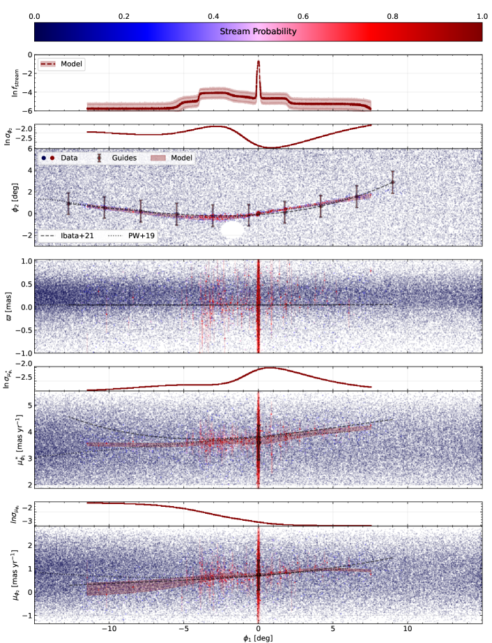
Figure 11: The model for Pal 5. For comparison we include the tracks from Price-Whelan et al. (2019) and Ibata et al. (2021). Panel 1: The stream mixture coefficients $f(\phi_{1})$ predicted by the model, colored by the stream membership likelihood. The stream fraction and number density drop to nearly $0$ for $\phi_{1}>5\ \rm{deg}$, making the track dominated by low-number statistics. Panel 2: $\phi_{2}(\phi_{1})$ over the full range of $\phi_{1}$. The data color and transparency are set by the model’s 50th-percentile stream probability. We include the error bars for stars with $>75\%$ membership probability. The predicted 50th-percentile track $\pm$ width is over-plotted (red band), along with the 90% confidence region (broader red bend). The 5th to 95th percentile variation in the width is shown in the adjoining top plot. Panel 3: $\varpi(\phi_{1})$ and $d(\phi_{1})$ over the full range of $\phi_{1}$. Panel 4 & 5: The proper motions $\mu_{\phi_{1}^{*}},\mu_{\phi_{2}}$. The model convolves observational errors with the stream width, but the large fractional errors make the determination difficult. The track is largely consistent with 0 width driven by small number statistics.

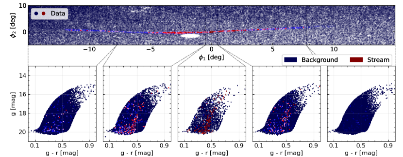
Figure 12: Photometric coordinate $(g,r)$ plots for each model component in 5 $\phi_{1}$ ranges across the data set, centered on the Pal 5 progenitor. On either side of the progenitor we strongly detect the stream for $\approx 5\degree$ and tentatively for an additional $\approx 5\degree$. The leading arm (positive $\phi_{1}$) track for $\phi_{1}>5\degree$ is consistent with Starkman et al. (2019). We do not detect any fanning of the stream, but given the shallow photometry, this is expected.

Table 4: Subset of Pal 5 Membership Table.
This table includes a selection of candidate member stars for the Pal 5 stream, based on the membership likelihoods. For each star we include the Gaia DR3 source ID and astrometric solution, the Pan-STARRS1 photometry, and the membership likelihoods for the stream and background. The likelihoods are computed using the trained model described in §​​ 5.3 and we include a quality flag ${\rm dim}(\boldsymbol{x})$, indicating the number of features used by the model. For most stars all features are measured. We use dropout regularization to estimate the uncertainty in the likelihoods, and report the 5% and 95% quantiles of the distribution, as well as the dropout-disabled maximum-likelihood estimate (MLE) of the likelihood.
We include as interesting cases:
$\phantom{+}\ast$  1 star with the highest MLE for the stream,
$\phantom{+}\ast$  5 stars with high stream MLE ($\mathcal{L}^{(S)}_{\rm MLE}>0.9$),
$\phantom{+}\ast$  4 stars with low stream MLE, but whose 95% likelihood is high ($\mathcal{L}^{(S)}_{\rm MLE}<0.75,\mathcal{L}^{(S)}_{\rm 95\%}>0.8$),
For convenience we round the likelihoods to 2 decimal places, and only show the value and uncertainty when it is non-zero.
The full table, including source ids, is available online.

Gaia					PS-1			Membership (${\rm MLE}_{5\%}^{95\%}$)
source_id	$\alpha$ [∘]	$\delta$ [∘]	$\mu_{\alpha}^{*}$ [$\frac{\rm{mas}}{\rm{yr}}$]	$\mu_{\delta}$ [$\frac{\rm{mas}}{\rm{yr}}$]	g [mag]	r [mag]	${\rm dim}(\boldsymbol{x})$	$\mathcal{L}_{\rm stream}$	$\mathcal{L}_{\rm background}$
—	228.98	-0.10	$-2.74\pm 0.04$	$-2.64\pm 0.03$	$15.99\pm 0.02$	$15.29\pm 0.02$	6	$1.00$	—
—	229.03	-0.03	$-2.77\pm 0.57$	$-1.92\pm 0.51$	$19.92\pm 0.02$	$19.55\pm 0.01$	6	$0.98_{-0.01}^{+0.01}$	$0.02_{-0.01}^{+0.01}$
—	228.97	-0.10	$-2.66\pm 0.74$	$-1.82\pm 0.65$	—	—	4	$0.99$	$0.01$
—	229.05	-0.20	$-3.44\pm 0.67$	$-2.77\pm 0.57$	$20.05\pm 0.01$	$19.67\pm 0.01$	6	$0.98_{-0.01}^{+0.00}$	$0.02_{-0.00}^{+0.01}$
—	229.00	-0.09	$-2.30\pm 0.59$	$-2.81\pm 0.51$	—	—	4	$1.00$	—
—	229.03	-0.13	$-1.52\pm 0.86$	$-3.60\pm 0.73$	—	—	4	$0.98_{-0.01}^{+0.00}$	$0.02_{-0.00}^{+0.01}$

Our fit to Pal 5 and its tidal tails is illustrated in Fig. 11. In the top panel we plot the stream fraction and its uncertainty, estimated by applying dropout during inference and evaluation of our model. The model clearly identifies the progenitor cluster $(\phi_{1}=0)$.

The membership probability of stream stars is illustrated in subsequent panels of Fig. 11, with guide points and their widths shown in red. The leading and trailing arms of the stream are clearly identified in our fits, with high membership probability on either side of the cluster. Our model prefers a thin on-sky morphology for Pal 5’s tidal tails, with an angular width of the stream (parameterized by $\ln{\sigma_{\phi_{2}}}$) around $\sim 0.1~{}\rm{deg}$. This is contrary to our fit of GD-1 in Fig. 6, where we find a more appreciable width of $\sim 0.2~{}\rm{deg}$ and above. This inferred width is consistent with Pal 5 being more distant than GD-1, though we expect a thin inferred width for Pal 5 since we do not model the stream in photometric coordinates. When photometry is available, we expect that our photometric model provides substantial constraining power in characterizing the stream, since diffuse parts of the tidal tails in on-sky angular coordinates remain tightly clustered in the CMD. This clustering is seen in our GD-1 fits (Fig. 7), where even the more extended parts of the stream remain clustered in the CMD.

The parallax, proper motion tracks, and their widths are also shown in Fig. 11. The red vertical lines represent the astrometric errors in each dimension, shown only for stars with membership probability greater than $75\%$. The errors are large compared to the width of the best fit stream track (shown as the red band). The track is a valid minimum to our loss function: because our model incorporates the large astrometric uncertainties, small variations to the estimated width of the stream in each dimension do not produce substantial changes to the loss function. Thus, a narrow stream in the kinematic dimensions provides a valid fit to the stream given the data at hand.

We also note that the track of the stream shown as the red band in each dimension appears to have an abrupt change in direction around $\phi_{1}\approx 7^{\circ}$. This also represents the region with the lowest stream fraction, as seen in the top panel of Fig. 11. In low stream fraction regions, the model is uncertain about the track of the stream since only a few stars contribute to the on-stream fit. The track changes highlight the importance of utilizing the membership probabilities of individual stars when analyzing any given stream, since membership probabilities incorporate information on the stream fraction while the mean stream-track alone does not provide this information.

In Fig. 12 we again show the data in $\phi_{1}-\phi_{2}$ coordinates, color-coded by membership probabilities in the top panel (same colorbar as in Fig. 11). In the bottom panels we plot the CMD of the data in bands of $\phi_{1}$. As discussed, our fit to Pal 5 does not incorporate information from the CMD. Thus, the bottom row represents a data-driven isochrone for Pal 5 and its tidal tails, obtained by fitting the stream’s astrometric overdensity. Indeed, the highest probability regions of the CMD appear qualitatively similar to a standard isochrone, with an extended and clustered sequence. The main sequence appears to be missing, which is expected given our cut at $G=20~{}\rm{mag}$, below which the main sequence of Pal 5 resides (Bonaca et al., 2020). The similarity of the color-magnitude distribution of Pal 5’s tidal tails to the red end of a standard isochrone highlights the validity of our astrometric membership model, since a photometric fit was never performed.

The stream solution, i.e. the per-star membership likelihood, is a posterior distribution. Fig. 11 and Fig. 12 show the membership likelihood evaluated at the $50$th percentile of this distribution, per star. In Fig. 13 we sample over the full distribution and smooth by a 0.1 deg (or mas/yr) kernel to produce a smooth representation of the stream. As a consequence of the sampling we see the model’s stream solution extends beyond the $\approx\pm 5\degree$ shown previously. Though the model certainty and individual membership likelihoods are low, the stream path matches closely with findings in deeper photometric catalogues, like Ibata et al. (2017).

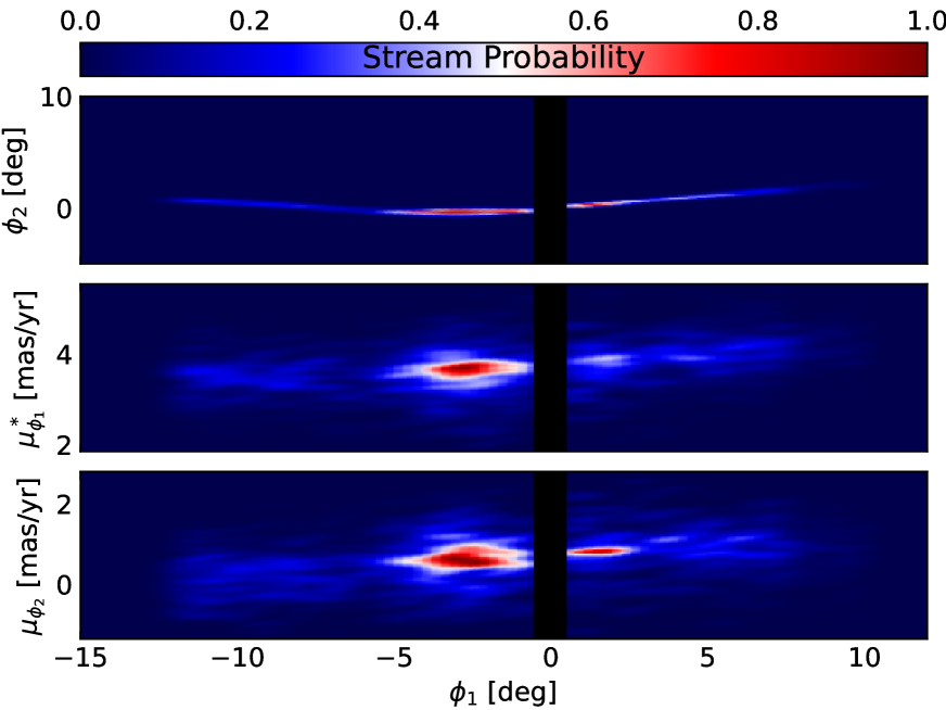
Figure 13: Smoothed KDE model of the stream’s member stars, weighted by their membership probability. The KDE has a bandwidth of $0.1\ \rm{deg}$ (or mas/yr). We exclude the progenitor to limit the density range and better display the diffuse tidal tails. The stream extends from $-12$ to $10$ degrees in this plot, which appears longer than in Fig. 11 and Fig. 12. Those show the membership likelihood at the $50$th-percentile of its distribution. This figure samples over the full posterior, showing the contribution of less-likely members.

While Gaia alone is not photometrically capable of observing the main sequence of Pal 5’s tidal tails, the modeling framework we present here is capable of operating on outer-joined datasets. This allows us to easily combine deep photometric data with kinematics from, e.g., Gaia. We leave that to a future work, though expect that a simultaneous model in photometry and astrometry would help identify the more diffuse parts of the stream, which become washed out in our astrometric fit due to the substantial number of background stars. Still, this section highlights the capability of our model when applied to a noisy field with a diffuse stream.

6 Discussion

We now provide a discussion of the methods presented in the paper, focusing on limitations of our approach in §​​ 6.1 and comparison to existing methods in §​​ 6.2. In §​​ 6.3 we discuss prospects for applying our method to existing and future datasets.

6.1 Caveats and Limitations

We now highlight the limitations of our method, and areas for potential improvement.

First, our usage of neural networks ensures that our method is expressive, and capable of describing a diverse range of stream morphologies all under one framework. At the same time, neural network training is computationally expensive, and takes a long time on a local device. Our fits to GD-1 and Pal 5 presented in this work were performed on a local computer without GPU support, though training time takes on the order of a few hours per stream. This can be improved substantially with the use of GPUs.

Second, our fits to GD-1 in §4 rely on a theoretical isochrone. While the stream does appear to be decently characterized by a theoretical isochrone, there is room for improvement. Especially considering that globular clusters do not always follow simple single-stellar population (see, e.g., Milone & Marino 2022 for a review of this subject), it is worth considering whether more data-driven approaches can be used to model the photometry of a stream without imposing tight priors on the stellar population.

Third, we have used a combination of analytic distributions and more flexible machine learning methods like normalizing flows to describe the distribution of background stars. However, the field of the Galaxy is complicated, in all coordinates. The analytic distributions in our modeling (specifically the $\phi_{2}$ background distributions) are clearly approximate. While the analytic distributions might be made more complex, the alternative is to substitute for non-parameteric flexible models. We have postponed this to future work, since the analytic backgrounds provide a decent description in the fields of GD-1 and Pal 5. However, this might not be the case for other streams. Constructing flexible background models will therefore provide further improvement over our method.

Fourth, the number density of stars belonging to a stream is determined by several interesting physical processes. These include (e.g.) epicyclic overdensities, the orbital phase of the stream, and interactions with galactic substructure. Our model constrains the stellar number density along any given stream, and can therefore be used to infer the underlying mechanism(s) responsible for the stream’s density. However, all observational surveys are subject to selection effects. In order to determine the nature and reality of a stream’s density fluctuations, selection effects must be accounted for. For the case of Gaia, there is ongoing work to model the survey’s selection function (Cantat-Gaudin et al., 2023). Our model provides the first step, which is to characterize the observations. With additional work, the selection function may be incorporated into our model and fits as a prior on the data. Doing so will enable a more robust analysis of each stream’s linear density, allowing us to make more definitive conclusions about its intrinsic structure. We defer this to future work

Finally, our method is suited for characterizing streams rather than detecting them. Thus, some amount of supervised work is required to reduce the data down to a clean enough selection of stars so that our model can converge to a high likelihood solution. Crucially, the field must contain not only stream stars but also enough background stars to model that component well and distinguish stream from background. As a rule of thumb, it is best if the stream is at least a few percent of the total data, preferably even 10%. Better background models permit this fraction to be pushed down further. If the field is too noisy and control points cannot be reliably placed, our method might not be able to characterize the stream of interest. This also applies to streams with bifurcated features like GD-1’s spur component. To model these additional features we must add a separate mixture component. A more data-driven approach to characterize previously unknown or diffuse extensions to a stream would mark a substantial improvement over our current implementation. We leave this to future work.

6.2 Comparison to Existing Methods

There are several existing methods for the detection of stellar streams, and some existing work on detailed stream characterization. Here we briefly overview the existing methods, and highlight commonalities and differences between the results of our work and previous studies.

Currently, the matched filter is the most common method for detecting and characterizing streams (e.g., Rockosi et al. 2002; Grillmair 2014; Bonaca et al. 2012; Jethwa et al. 2018; Shipp et al. 2018). The method works by selecting a stellar population in the CMD (i.e., from a metal-poor isochrone) and searching for a stellar overdensity in the astrometric data. The approach has proved successful for stream detection, but to a lesser extent for characterization. From the matched filter approach alone, stream membership probabilities are not obtained and there is substantial contamination from background stars. While the approach can provide an excellent coarse-grained description of a given stream, it does not provide a density model in astrometry and photometry.

To a good approximation streams are expected to roughly trace a stellar orbit. The STREAMFINDER algorithm exploits this physical expectation (Malhan & Ibata, 2018), by integrating orbits in a trial Galactic potential and identifying stellar overdensities that appear to coincide with segments of the trial orbits. While the method has identified many stream candidates, using these streams for potential reconstruction is circular in reasoning. That is, the detection and characterization of these streams is conditioned on a choice of the potential. The method we present here does not make assumptions about the gravitational potential, nor do we enforce physical assumptions about the dynamics of each stream.

This work represents one machine learning-based approach for stream characterization. Another method is presented in Shih et al. (2022), VIA MACHINAE, which uses conditional density estimation and a linear feature detector to discover streams and identify probable members. While the method is promising for stream discovery, its intended use is not for detailed characterization (as stated in Shih et al. 2022). Our work has the opposite intent: the method presented is not designed to detect streams, rather, it is well-suited for characterizing streams that fall within some predefined field. Thus, our method can be used for characterizing the VIA MACHINAE candidates, and obtaining more robust membership probabilities.

In Patrick et al. (2022) the stellar density of 13 tidal streams is modeled in on-sky positions and color-magnitude coordinates. The morphology of each stream is characterized by a series of splines, which are themselves a function of $\phi_{1}$. This method was originally developed in Erkal et al. (2017). Importantly, Patrick et al. (2022) performs a fit in $\phi_{1}-\phi_{2}$ and photometry, similar to our work. The photometric approach in Patrick et al. (2022) relies on generating mock stellar populations in the CMD, selecting probable stream stars, modeling the $\phi_{1}-\phi_{2}$ distribution for those stars, and then refining the CMD fit based on the $\phi_{1}-\phi_{2}$ fit. This approach is therefore similar to a matched filter analysis. The model does not currently incorporate kinematic information, though the work could be extended. The improvement of our work is that we do not require an iterative fit to the CMD and astrometry: we handle both spaces through a joint likelihood without simulating mock-observations. Additionally, we can easily incorporate kinematic information and data with missing phase-space dimensions.

We also highlight upcoming work from the CATS Collaboration 2023 (in prep.), which provides a spline-based characterization of streams implemented in the Jax library (Bradbury et al., 2018). The Jax backend ensures that fitting the model to a stream is very fast (on the order of minutes), and also has the capability of incorporating kinematic data with missing phase-space dimensions. The method does not currently model the color-magnitude distribution of a stream, but relies on a loose photometric selection. The photometric model in this work could be extended to the spline-based method, allowing for a joint astrometric and photometric model than can be rapidly fit to the stream of interest.

In total, having multiple methods to characterize streams and their membership probabilities is advantageous. As the volume of tidal features continues to grow, it will become important to fit different models to the same stream, in order to evaluate whether certain features or density variations are real versus spurious artifacts from the adopted method. Considering the information encoded about perturbations in the small-scale density fluctuations along a given stream, a posterior distribution over models will help capture systematic errors in our description of streams and the field of perturbations that give rise to their density.

6.3 Combining Information from Present and Future Surveys

Streams have been primarily discovered and characterized using photometric searches and matched filter methods (e.g., Rockosi et al. 2002; Grillmair 2014; Bonaca et al. 2012; Jethwa et al. 2018; Shipp et al. 2018). Gaia has enabled a more precise localization of streams, thanks to their compact kinematic distribution relative to a field of background stars. On the other hand, Gaia is not photometrically deep ($G\lesssim 21$) and therefore is less sensitive to diffuse streams in the outer Milky Way halo. Current and upcoming surveys — e.g., DES (Abbott et al., 2018, 2021), Euclid (Laureijs et al., 2011), Rubin (Ivezić et al., 2019), Roman (Spergel et al., 2013) — do and will probe much deeper photometrically than Gaia can detect. From the more distant stellar halo (Shipp et al., 2018) to extragalactic systems (Martínez-Delgado et al., 2008; Demirjian et al., 2020; Román et al., 2023), these missions will reveal many new tidal features. Since Gaia cannot be used for these streams, kinematic information will be rare, requiring dedicated followup observations.

In this work we build mixture models (specifically MDNs) to characterize streams using all of the existing photometric and astrometric data for a given field. Looking to Fig. 6 and Fig. 11, the proper motion components of the model are among the most information-rich and contribute significantly to the model. What then are the prospects for using this work with streams discovered with data from DES, Euclid, Rubin, etc? There are two categories of streams these surveys will observe. The first is streams that partially appear in Gaia but are deeper in these surveys; Pal 5 is an example, with its main sequence below the Gaia observation limit. Our method permits missing phase-space dimensions, therefore allowing “outer”-joined catalogues mixing Gaia and photometrically deeper surveys. In this scenario the stream track in proper motions and parallaxes (and possibly radial velocities) communicate and are mutually constrained with the photometric tracks. The second category is streams entirely missing from Gaia, where the data is on-sky positions ($\phi_{1}$, $\phi_{2}$), photometry ($\boldsymbol{m}$), and potentially metallicities. Even in this limited data regime, our stream characterization framework is applicable. The normalizing flow background model with a tightly constrained stream isochrone model can be flexibly applied to any stream, allowing for a characterization of the tidal feature insofar as the available data allows.

The ability to simultaneously model the on-sky and photometric distribution of a stream makes this approach a quantitative and Bayesian form of a matched filter analysis. For this reason, our method is readily applicable to the wealth of data expected from upcoming surveys, including both streams discovered in the Milky Way and extragalactic tidal features. While the present work is concerned with the former case, similar methods to the approach developed here may be applied to extragalactic tidal features, 1000s of which are expected to be discovered with Rubin (Ivezić et al., 2019) and Roman (Spergel et al., 2013). With a density model of an extragalactic tidal feature, the gravitational potential of external galaxies can be constrained (e.g., Fardal et al. 2013; Pearson et al. 2022; Nibauer et al. 2023). We leave an extension of our method to extragalactic streams to future work.

7 Summary and Conclusion

We have constructed and demonstrated a new method for characterizing stellar streams, given all of the astrometric and photometric data available. We model a stream in astrometric coordinates using mixture density networks, allowing for a flexible representation of diverse stream morphologies under a single modeling framework. Additionally, our astrometric fit does not rely on assumptions about the gravitational potential. Our simultaneous photometric model treats each stream as a single-stellar population, generated from a theoretical isochrone. The distance modulus along the stream is itself a function of $\phi_{1}$, allowing us to tie photometric information to parallax measurements along the stream. This tie enables a reconstruction of stellar stream distance tracks that are compatible with photometry and astrometry by construction. A joint model in astrometric and photometric coordinates also naturally allows for more spatially diffuse regions of a stream to be detected. Additionally, our background model relies on a combination of analytic densities and normalizing flows, each of which are modular in StreamMapper and readily adaptable to a given field.

The combination of a flexible stream and background model allows us to obtain robust stream-membership probabilities for each star in a given field. This enables the generation of statistical samples for stream stars, informed by astrometry and photometry. We apply the method to the stream GD-1 and the tidal tails of Palomar 5, generating membership catalogs for both streams that are publicly available at zenodo:10211410. Our characterization of GD-1 reveals a significant detection of the stream’s main component as well as the “spur” component, which represents a bifurcation from the main stream. We also recover density variations and gaps along the stream that have been previously observed. Our fit to Pal 5 demonstrates the performance of our model on a more diffuse stream with low signal-to-noise measurements. The inclusion of deeper photometric data for Pal 5 will enable a more extended view of the stream.

Our method represents a new avenue to characterize the growing census of stellar streams discovered in the Milky Way. While most streams have been roughly characterized with matched filter algorithms, a statistical and homogeneous determination of stream-membership probabilities for each star has not been performed or made publicly available. A homogeneous catalog of stellar streams and stellar membership probabilities will therefore represent a substantial step forward for modeling the Galaxy, since both the global track of a stream and its small-scale density distribution are sensitive to the Milky Way’s gravitational potential.

Especially when considering the small-scale perturbation history of a stream predicted by $\Lambda\rm{CDM}$, the inclusion or exclusion of stream stars can make a substantial difference in our inference of the perturbers. Constructing catalogs with membership probabilities as we do in this work provides a crucial step forward to making our inference of, e.g., dark matter subhalos in the Galaxy more robust. Equipped with membership probabilities, one is finally able to propagate the uncertainty in our determination of the “on-stream data” through to the posterior distribution of model parameters (e.g., those characterizing the subhalo mass function). Thus, our works provides a new technique to generate samples of stream stars using all of the existing kinematic and photometric data, from which models for the Milky Way and its potential can be constrained in a statistically sound manner.

8 acknowledgements

NS acknowledges support from the Natural Sciences and Engineering Research Council of Canada (NSERC) - Canadian Graduate Scholarships Doctorate Program [funding reference number 547219 - 2020]. NS received partial support from NSERC (funding reference number RGPIN-2020-04712) and from an Ontario Early Researcher Award (ER16-12-061; PI Bovy).

JN is supported by a National Science Foundation Graduate Research Fellowship, Grant No. DGE-2039656. Any opinions, findings, and conclusions or recommendations expressed in this material are those of the author(s) and do not necessarily reflect the views of the National Science Foundation.

Both NS and JN would like to thank the Community Atlas of Tidal Streams 2022 conference for starting the discussions that led to this work. We thank Joshua Speagle for conversations and suggestions that were crucial to the development of the photometric model. We also thank Shirley Ho and Miles Cranmer for insightful discussions and comments.

This work has made use of data from the European Space Agency (ESA) mission Gaia (https://www.cosmos.esa.int/gaia), processed by the Gaia Data Processing and Analysis Consortium (DPAC, https://www.cosmos.esa.int/web/gaia/dpac/consortium). Funding for the DPAC has been provided by national institutions, in particular the institutions participating in the Gaia Multilateral Agreement.

The data availability statement is modified from one provided to ShowYourWork by Mathieu Renzo.

Software (alphabetical)

asdf (Greenfield et al., 2015), astropy (Astropy Collaboration et al., 2013, 2018, 2022), astroquery (Ginsburg et al., 2019), brutus (Speagle et al., 2020), Matplotlib (Hunter, 2007), NumPy (Harris et al., 2020), Pytorch (Paszke et al., 2019), SciPy (Virtanen et al., 2020), ShowYourWork (Luger et al., 2021), zuko (Rozet, 2023).

Data Availability

This study was carried out using the reproducibility software (Luger et al., 2021), which uses continuous integration to programmatically download the data, perform the analyses, create the figures, and compile the manuscript. Each figure caption contains two links: one to the dataset used in the corresponding figure, and the other to the script used to make the figure. The datasets are stored at zenodo:10211410. The git repository associated with this study is publicly available at nstarman/stellar_stream_density_ml_paper. The open-source code base developed for this project is StreamMapper.

Appendix A Probability Distributions

A variety of probability distributions are used when modeling the stream and Galactic background. This appendix presents relevant mathematical details of these distributions. In particular, observational errors are modeled as Gaussian distributions, which requires modifying each distribution to account for the Gaussian noise.

Let $x\sim X$ be distributed as some specified distribution and $\delta\sim\Delta\equiv\mathcal{N}(0,\sigma_{*})$ as an independent, centered Gaussian. An observation $Y$ is distributed as

$$Z=X+\Delta,$$ (A1)

Which is a convolution of the PDFs.

$$p_{Z}(x;\boldsymbol{\theta},\sigma) \equiv(p_{X}(x;\boldsymbol{\theta})*\mathcal{N}(x;0,\sigma))$$ (A2)

$$=\int_{-\infty}^{\infty}\rm{d}\tau\,p(x;\boldsymbol{\theta})\mathcal{N}(x-\tau;0,\sigma)$$ (A3)

In the following subsections we work through the distributions $p(x,\boldsymbol{\theta})$ and the convolutions with $\mathcal{N}(x,0,{\sigma_{*}})$.

A.1 Flat Distribution

The simplest distribution is that of the univariate uniform distribution. For a domain $x\in[a,b]$ the PDF is given by

$$P_{\mathcal{U}}(x|a,b)=\begin{cases}(b-a)^{-1}&a<x\leq b\\ 0&\text{else}\end{cases}$$ (A4)

where $a,b$ are the bounds.

In practice, the bounds $a,b$ are the bounds of the observation window, creating a subset of a larger field. Suppose the larger field is uniformly distributed in a region larger than the bounds $a,b$, ie. $P_{\mathcal{U}}(x|\alpha,\beta)$. Let each observed datum $x_{n}$ in the field have Gaussian error ${\sigma_{*}}_{n}$, then the PDF of the uniform-Gaussian-convolved distribution is given by:

$$p_{(\mathcal{U}*\mathcal{N})}(x;\alpha,\beta,{\sigma_{*}})=\begin{cases}p_{\mathcal{U}}(x;\alpha,\beta)\left(P_{\mathcal{N}}(x;\alpha,{\sigma_{*}})-P_{\mathcal{N}}(x;\beta,{\sigma_{*}})\right)&\alpha\leq x\leq\beta\\ 0&\text{else}\end{cases}$$ (A5)

We then truncate this distribution to the observed field $(a,b]$

$$p_{(\mathcal{U}*\mathcal{N})}(x|a<X\leq b;\alpha,\beta,{\sigma_{*}})$$ (A6)

in the normal fashion: setting $p_{(\mathcal{U}*\mathcal{N})}=0$ when $x<a,x>b$ and normalizing $p_{(\mathcal{U}*\mathcal{N})}$ within $(a,b]$. The truncated distribution is tractable but unwieldy. The distribution can be simplified enormously if two conditions hold: first, $\alpha\ll a,b\ll\beta$, the observed field is a small subset of the full field; and second, ${\sigma_{*}}\ll|\alpha-a|$ and ${\sigma_{*}}\ll|\beta-b|$, the errors are smaller than the observation window size compared to the full field. In this case, the distribution reduces back to the uniform distribution!

Therefore, for all cases considered in this work (A6) becomes:

$$p_{(\mathcal{U}*\mathcal{N})}(x|a<X\leq b;\alpha,\beta,{\sigma_{*}})\cong P_{\mathcal{U}}(x|a,b)$$ (A7)

A.2 Truncated Exponential Distribution

The univariate exponential distribution is:

$$p_{\mathcal{E}}(x;\lambda)=\begin{cases}me^{-\lambda x}&x\in[0,\infty)\\ 0&x<0\end{cases}$$ (A8)

The support of this distribution, $[0,\infty)$, rarely matches the support of the data. We generalize to the unit-normalized, truncated, univariate exponential distribution in the domain $(a,b]$:

$$p_{\mathcal{E}_{T}}(x;\lambda,a,b)=\begin{cases}\frac{\lambda e^{-\lambda\,(x-a))}}{1-e^{-\lambda(b-a)}}&a<x\leq b\\ 0&\text{else},\end{cases}$$ (A9)

for bounds $x\in(a,b]$. However, as $\lambda\rightarrow 0$, which describes the flat distribution (§​​ A.1), this functional form can be numerically unstable. It is therefore practical to define $p_{\mathcal{E}}(x;|\lambda|<\epsilon,a,b)\cong P_{\mathcal{U}}(x;a,b)$.

Let each observed datum $x_{n}$ in the field have Gaussian error ${\sigma_{*}}_{n}$, then the PDF of the Exponential-convolved-with-a-Gaussian distribution is given by:

$$p_{\mathcal{E}\cdot\mathcal{N}}(x;m,a,\sigma_{*})=\frac{me^{\frac{1}{2}\lambda\left(2b+\lambda\sigma_{*}^{2}-2x\right)}}{e^{\lambda(b-a)}-1}=p_{\mathcal{E}}(x;\lambda,a)\ e^{\frac{1}{2}\lambda^{2}\sigma_{*}^{2}},$$ (A10)

where the function is no longer truncated, since a Gaussian is not compact.

We impose the same observation field $(a,b]$ and truncate $p_{\mathcal{E}\cdot\mathcal{N}}(x|a<X\leq b;m,a,\sigma_{*})$. We note the normalization, which is the CDF evaluated at $a,b$, cancels the factor $e^{\frac{1}{2}\lambda^{2}\sigma_{*}^{2}}$. Following thtough, the truncated convolved distribution is identical to the original distribution.

$$p_{(\mathcal{E}\cdot\mathcal{N})_{T}}x|a<X\leq b;m,a,\sigma_{*})\equiv p_{\mathcal{E}}(x;\lambda,a,b)$$ (A11)

A.3 Normal Distribution

The properties of the Normal distribution are well known. For completeness we state

$$P_{X}(x;\mu,\sigma)=\mathcal{N}(x;\mu,\sigma).$$ (A12)

With the inclusion of observational errors the distribution becomes

$$P_{\mathcal{N}\cdot\mathcal{N}}(x;\mu,\sigma,{\sigma_{*}})=\mathcal{N}(x;\mu,\sqrt{\sigma^{2}+{\sigma_{*}}^{2}}).$$ (A13)

The Normal distribution is not compact, with non-zero value over all $x$. In an observational window $(a,b]$ the PDF is truncated, giving

$$P_{\mathcal{N}_{T}}(x;\mu,\sigma,a,b)=\begin{cases}\frac{\mathcal{N}(x;\mu,\sigma)}{\Phi_{\mathcal{N}}(b;\mu,\sigma)-\Phi_{\mathcal{N}}(a;\mu,\sigma)}&a<x\leq b\\ 0&\text{else}\end{cases}$$ (A14)

Note that the observation-window-truncation is performed on the full distribution, which includes the observational errors, if present. Therefore, let $\tilde{\sigma}^{2}\equiv\sigma^{2}+\sigma_{*}^{2}$

$$P_{(\mathcal{N}\cdot\mathcal{N})_{T}}(x;\mu,\tilde{\sigma},a,b)=P_{\mathcal{N}_{T}}(x;\mu,\tilde{\sigma},a,b)$$ (A15)

Appendix B Pairing Neural Networks with Priors

In modeling, the choices of priors are important, not only for the information they adds to a model, but also for how optimizers explore parameter spaces. Simple optimizers, like MCMC, propose a parameter vector then compute its likelihood given the data (Hogg & Foreman-Mackey, 2018). Priors with compact support $\theta\sim\mathcal{D}((a,b])$, e.g. $\mathcal{U}(a,b)$, may be very dangerous as the optimizer can be initialized in a region with zero probability and has no means but blind luck to find the region of support – the region with non-zero likelihood. More sophisticated optimizers, like gradient-based descent (Cauchy, 1847), are susceptible to a similar initialization problem, allowing zero-probability regions, but requiring at least a non-zero gradient to make informed updates to the optimizers state. Outside the support the gradient can be zero. With MDNs, model parameters are neural network outputs. Unlike for conventional models where an informed initial parameter state may be chosen by hand, it is impractical and undesirable to initialize by hand a neural network’s output by setting all its internal weights. One might imagine accomplishing a desired initial output by pre-training the network with a toy model that forces convergence on a set output vector. However, neural networks are highly non-linear in their response to internal state changes (a desirable property). It is quite possible that when switching from the toy to real model’s loss function the pre-trained network is in a local probability island from which the global optimum is unreachable. Therefore, with the MDN neural networks, initialization is mostly for checking the dependence of the results on the initial state – though even this dependence may instead be done using parameter dropout. Rather than focusing on initializing to a particular parameter vector, for neural networks it is instead important that the initial state, whatever it is, has non-zero probability (or non-zero gradient, depending on the optimizer). Neural networks have some intrinsic phase-space range that depends on the architecture of the network. Therefore the network architecture must be chosen such that the outputs match well with the priors. For example, with a uniform prior $\theta\sim\mathcal{U}(a,b)$, the network should be restricted such that $\theta\in(a,b]$, e.g. by ending the network’s $\theta$ channel with a scaled logistic function.

References

- Abbott et al. (2018) Abbott, T. M. C., Abdalla, F. B., Allam, S., et al. 2018, ApJS, 239, 18, doi: 10.3847/1538-4365/aae9f0
- Abbott et al. (2021) Abbott, T. M. C., Adamów, M., Aguena, M., et al. 2021, ApJS, 255, 20, doi: 10.3847/1538-4365/ac00b3
- Aggarwal et al. (2002) Aggarwal, C., Hinneburg, A., & Keim, D. 2002, First publ. in: Database theory, ICDT 200, 8th International Conference, London, UK, January 4 - 6, 2001 / Jan Van den Bussche … (eds.). Berlin: Springer, 2001, pp. 420-434 (=Lecture notes in computer science ; 1973)
- Antoja et al. (2020) Antoja, T., Ramos, P., Mateu, C., et al. 2020, A&A, 635, L3, doi: 10.1051/0004-6361/201937145
- Antoja et al. (2014) Antoja, T., Helmi, A., Dehnen, W., et al. 2014, A&A, 563, A60, doi: 10.1051/0004-6361/201322623
- Arias et al. (1997) Arias, E. F., Charlot, P., Feissel, M., & Lestrade, J. F. 1997, IERS Technical Note, 23, IV
- Astropy Collaboration et al. (2013) Astropy Collaboration, Robitaille, T. P., Tollerud, E. J., et al. 2013, A&A, 558, A33, doi: 10.1051/0004-6361/201322068
- Astropy Collaboration et al. (2018) Astropy Collaboration, Price-Whelan, A. M., Sipőcz, B. M., et al. 2018, AJ, 156, 123, doi: 10.3847/1538-3881/aabc4f
- Astropy Collaboration et al. (2022) Astropy Collaboration, Price-Whelan, A. M., Lim, P. L., et al. 2022, ApJ, 935, 167, doi: 10.3847/1538-4357/ac7c74
- Bennett & Bovy (2019) Bennett, M., & Bovy, J. 2019, MNRAS, 482, 1417, doi: 10.1093/mnras/sty2813
- Binney (2008) Binney, J. 2008, MNRAS, 386, L47, doi: 10.1111/j.1745-3933.2008.00458.x
- Bishop (1994a) Bishop, C. 1994a, Mixture density networks, Workingpaper, Aston University
- Bishop (1994b) —. 1994b, Mixture density networks, Workingpaper, Aston University
- Bishop (2016) Bishop, C. M. 2016, Pattern Recognition and Machine Learning (Information Science and Statistics), paperback edn. (Springer), 758. https://lead.to/amazon/com/?op=bt&la=en&cu=usd&key=1493938436
- Bonaca et al. (2012) Bonaca, A., Geha, M., & Kallivayalil, N. 2012, ApJ, 760, L6, doi: 10.1088/2041-8205/760/1/L6
- Bonaca et al. (2014) Bonaca, A., Geha, M., Küpper, A. H. W., et al. 2014, ApJ, 795, 94, doi: 10.1088/0004-637X/795/1/94
- Bonaca et al. (2019) Bonaca, A., Hogg, D. W., Price-Whelan, A. M., & Conroy, C. 2019, ApJ, 880, 38, doi: 10.3847/1538-4357/ab2873
- Bonaca et al. (2020) Bonaca, A., Pearson, S., Price-Whelan, A. M., et al. 2020, ApJ, 889, 70, doi: 10.3847/1538-4357/ab5afe
- Bovy (2014) Bovy, J. 2014, ApJ, 795, 95, doi: 10.1088/0004-637X/795/1/95
- Bovy et al. (2016) Bovy, J., Bahmanyar, A., Fritz, T. K., & Kallivayalil, N. 2016, ApJ, 833, 31, doi: 10.3847/1538-4357/833/1/31
- Bovy et al. (2017) Bovy, J., Erkal, D., & Sanders, J. L. 2017, MNRAS, 466, 628, doi: 10.1093/mnras/stw3067
- Bradbury et al. (2018) Bradbury, J., Frostig, R., Hawkins, P., et al. 2018, JAX: composable transformations of Python+NumPy programs, 0.3.13. http://github.com/google/jax
- Cantat-Gaudin et al. (2023) Cantat-Gaudin, T., Fouesneau, M., Rix, H.-W., et al. 2023, A&A, 669, A55, doi: 10.1051/0004-6361/202244784
- Carlberg (2012) Carlberg, R. G. 2012, ApJ, 748, 20, doi: 10.1088/0004-637X/748/1/20
- Carlberg & Grillmair (2013) Carlberg, R. G., & Grillmair, C. J. 2013, ApJ, 768, 171, doi: 10.1088/0004-637X/768/2/171
- Cauchy (1847) Cauchy, A.-L. 1847, Cambridge Library Collection - Mathematics, Vol. 10, ANALYSE MATHÉMATIQUE. – Méthodc générale pour la résolution des systèmes d’équations simultanées (Cambridge University Press), 399–402, doi: 10.1017/CBO9780511702396.063
- Chambers et al. (2016) Chambers, K. C., Magnier, E. A., Metcalfe, N., et al. 2016, arXiv e-prints, arXiv:1612.05560, doi: 10.48550/arXiv.1612.05560
- Choi et al. (2016) Choi, J., Dotter, A., Conroy, C., et al. 2016, ApJ, 823, 102, doi: 10.3847/0004-637X/823/2/102
- de Boer et al. (2018) de Boer, T. J. L., Belokurov, V., Koposov, S. E., et al. 2018, MNRAS, 477, 1893, doi: 10.1093/mnras/sty677
- de Boer et al. (2020) de Boer, T. J. L., Erkal, D., & Gieles, M. 2020, MNRAS, 494, 5315, doi: 10.1093/mnras/staa917
- Dehnen et al. (2004) Dehnen, W., Odenkirchen, M., Grebel, E. K., & Rix, H.-W. 2004, AJ, 127, 2753, doi: 10.1086/383214
- Demirjian et al. (2020) Demirjian, A., Pearson, S., & Clark, S. 2020, in American Astronomical Society Meeting Abstracts, Vol. 235, American Astronomical Society Meeting Abstracts #235, 371.18
- Dirac (1947) Dirac, P. A. M. 1947, The principles of quantum mechanics (Oxford University Press)
- Dotter (2016) Dotter, A. 2016, ApJS, 222, 8, doi: 10.3847/0067-0049/222/1/8
- Erkal et al. (2017) Erkal, D., Koposov, S. E., & Belokurov, V. 2017, MNRAS, 470, 60, doi: 10.1093/mnras/stx1208
- Fardal et al. (2013) Fardal, M. A., Weinberg, M. D., Babul, A., et al. 2013, MNRAS, 434, 2779, doi: 10.1093/mnras/stt1121
- Gaia Collaboration (2023) Gaia Collaboration. 2023, Gaia Data Release 3 Completeness of source contents, Gaia Collaboration. https://gea.esac.esa.int/archive/documentation/GDR3/Catalogue_consolidation/chap_cu9val/sec_cu9val_introduction/ssec_cu9val_intro_completeness.html
- Gaia Collaboration et al. (2016a) Gaia Collaboration, Prusti, T., de Bruijne, J. H. J., et al. 2016a, A&A, 595, A1, doi: 10.1051/0004-6361/201629272
- Gaia Collaboration et al. (2016b) —. 2016b, A&A, 595, A1, doi: 10.1051/0004-6361/201629272
- Gaia Collaboration et al. (2023a) Gaia Collaboration, Vallenari, A., Brown, A. G. A., et al. 2023a, A&A, 674, A1, doi: 10.1051/0004-6361/202243940
- Gaia Collaboration et al. (2023b) —. 2023b, A&A, 674, A1, doi: 10.1051/0004-6361/202243940
- Gal & Ghahramani (2015) Gal, Y., & Ghahramani, Z. 2015, arXiv e-prints, arXiv:1506.02157, doi: 10.48550/arXiv.1506.02157
- Ginsburg et al. (2019) Ginsburg, A., Sipőcz, B. M., Brasseur, C. E., et al. 2019, AJ, 157, 98, doi: 10.3847/1538-3881/aafc33
- GRAVITY Collaboration et al. (2018) GRAVITY Collaboration, Abuter, R., Amorim, A., et al. 2018, A&A, 615, L15, doi: 10.1051/0004-6361/201833718
- Green (2018) Green, G. 2018, The Journal of Open Source Software, 3, 695, doi: 10.21105/joss.00695
- Green et al. (2019) Green, G. M., Schlafly, E., Zucker, C., Speagle, J. S., & Finkbeiner, D. 2019, ApJ, 887, 93, doi: 10.3847/1538-4357/ab5362
- Greenfield et al. (2015) Greenfield, P., Droettboom, M., & Bray, E. 2015, Astronomy and Computing, 12, 240, doi: 10.1016/J.ASCOM.2015.06.004
- Grillmair (2014) Grillmair, C. J. 2014, ApJ, 790, L10, doi: 10.1088/2041-8205/790/1/L10
- Grillmair & Dionatos (2006a) Grillmair, C. J., & Dionatos, O. 2006a, ApJ, 643, L17, doi: 10.1086/505111
- Grillmair & Dionatos (2006b) —. 2006b, ApJ, 641, L37, doi: 10.1086/503744
- Grillmair et al. (1995) Grillmair, C. J., Freeman, K. C., Irwin, M., & Quinn, P. J. 1995, AJ, 109, 2553, doi: 10.1086/117470
- Grillmair & Johnson (2006) Grillmair, C. J., & Johnson, R. 2006, ApJ, 639, L17, doi: 10.1086/501439
- Grillmair & Smith (2001) Grillmair, C. J., & Smith, G. H. 2001, AJ, 122, 3231, doi: 10.1086/323916
- Harris et al. (2020) Harris, C. R., Millman, K. J., van der Walt, S. J., et al. 2020, Nature, 585, 357, doi: 10.1038/s41586-020-2649-2
- Harris (1996) Harris, W. E. 1996, AJ, 112, 1487, doi: 10.1086/118116
- Hattori et al. (2016) Hattori, K., Erkal, D., & Sanders, J. L. 2016, MNRAS, 460, 497, doi: 10.1093/mnras/stw1006
- Hermans et al. (2021) Hermans, J., Banik, N., Weniger, C., Bertone, G., & Louppe, G. 2021, MNRAS, 507, 1999, doi: 10.1093/mnras/stab2181
- Hogg & Foreman-Mackey (2018) Hogg, D. W., & Foreman-Mackey, D. 2018, ApJS, 236, 11, doi: 10.3847/1538-4365/aab76e
- Hunter (2007) Hunter, J. D. 2007, Computing in Science and Engineering, 9, 90, doi: 10.1109/MCSE.2007.55
- Ibata et al. (2020) Ibata, R., Thomas, G., Famaey, B., et al. 2020, ApJ, 891, 161, doi: 10.3847/1538-4357/ab7303
- Ibata et al. (2021) Ibata, R., Malhan, K., Martin, N., et al. 2021, ApJ, 914, 123, doi: 10.3847/1538-4357/abfcc2
- Ibata et al. (2002) Ibata, R. A., Lewis, G. F., Irwin, M. J., & Quinn, T. 2002, MNRAS, 332, 915, doi: 10.1046/j.1365-8711.2002.05358.x
- Ibata et al. (2016) Ibata, R. A., Lewis, G. F., & Martin, N. F. 2016, ApJ, 819, 1, doi: 10.3847/0004-637X/819/1/1
- Ibata et al. (2017) Ibata, R. A., Lewis, G. F., Thomas, G., Martin, N. F., & Chapman, S. 2017, ApJ, 842, 120, doi: 10.3847/1538-4357/aa7514
- Ibata et al. (1998) Ibata, R. A., Lewis, G. F., Totten, E., & Irwin, M. J. 1998, in Dynamical Studies of Star Clusters and Galaxies, ed. P. Kroupa, J. Palous, & R. Spurzem, 178
- Ivezić et al. (2019) Ivezić, Ž., Kahn, S. M., Tyson, J. A., et al. 2019, ApJ, 873, 111, doi: 10.3847/1538-4357/ab042c
- Jethwa et al. (2018) Jethwa, P., Torrealba, G., Navarrete, C., et al. 2018, MNRAS, 480, 5342, doi: 10.1093/mnras/sty2226
- Jimenez Rezende & Mohamed (2015) Jimenez Rezende, D., & Mohamed, S. 2015, arXiv e-prints, arXiv:1505.05770, doi: 10.48550/arXiv.1505.05770
- Johnston et al. (2002) Johnston, K. V., Spergel, D. N., & Haydn, C. 2002, ApJ, 570, 656, doi: 10.1086/339791
- Johnston et al. (1999) Johnston, K. V., Zhao, H., Spergel, D. N., & Hernquist, L. 1999, ApJ, 512, L109, doi: 10.1086/311876
- Kobyzev et al. (2019) Kobyzev, I., Prince, S. J. D., & Brubaker, M. A. 2019, arXiv e-prints, arXiv:1908.09257, doi: 10.48550/arXiv.1908.09257
- Koposov et al. (2010) Koposov, S. E., Rix, H.-W., & Hogg, D. W. 2010, ApJ, 712, 260, doi: 10.1088/0004-637X/712/1/260
- Koposov et al. (2019) Koposov, S. E., Belokurov, V., Li, T. S., et al. 2019, MNRAS, 485, 4726, doi: 10.1093/mnras/stz457
- Koposov et al. (2023) Koposov, S. E., Erkal, D., Li, T. S., et al. 2023, MNRAS, 521, 4936, doi: 10.1093/mnras/stad551
- Kroupa (2001) Kroupa, P. 2001, MNRAS, 322, 231, doi: 10.1046/j.1365-8711.2001.04022.x
- Küpper et al. (2012) Küpper, A. H. W., Lane, R. R., & Heggie, D. C. 2012, MNRAS, 420, 2700, doi: 10.1111/j.1365-2966.2011.20242.x
- Laureijs et al. (2011) Laureijs, R., Amiaux, J., Arduini, S., et al. 2011, arXiv e-prints, arXiv:1110.3193, doi: 10.48550/arXiv.1110.3193
- Leung et al. (2022) Leung, H. W., Bovy, J., Mackereth, J. T., et al. 2022, arXiv e-prints, arXiv:2204.12551. https://arxiv.org/abs/2204.12551
- Li et al. (2019) Li, T. S., Koposov, S. E., Zucker, D. B., et al. 2019, MNRAS, 490, 3508, doi: 10.1093/mnras/stz2731
- Li et al. (2022) Li, T. S., Ji, A. P., Pace, A. B., et al. 2022, ApJ, 928, 30, doi: 10.3847/1538-4357/ac46d3
- Lindegren et al. (2021) Lindegren, L., Bastian, U., Biermann, M., et al. 2021, A&A, 649, A4, doi: 10.1051/0004-6361/202039653
- Luger et al. (2021) Luger, R., Bedell, M., Foreman-Mackey, D., et al. 2021, arXiv e-prints, arXiv:2110.06271. https://arxiv.org/abs/2110.06271
- Majewski et al. (2003) Majewski, S. R., Skrutskie, M. F., Weinberg, M. D., & Ostheimer, J. C. 2003, ApJ, 599, 1082, doi: 10.1086/379504
- Malhan & Ibata (2018) Malhan, K., & Ibata, R. A. 2018, MNRAS, 477, 4063, doi: 10.1093/mnras/sty912
- Martínez-Delgado et al. (2008) Martínez-Delgado, D., Peñarrubia, J., Gabany, R. J., et al. 2008, ApJ, 689, 184, doi: 10.1086/592555
- Mateu (2022) Mateu, C. 2022, arXiv e-prints, arXiv:2204.10326. https://arxiv.org/abs/2204.10326
- McLachlan & Basford (1989) McLachlan, G. J., & Basford, K. E. 1989, in Mixture models : inference and applications to clustering. https://api.semanticscholar.org/CorpusID:119405289
- Milone & Marino (2022) Milone, A. P., & Marino, A. F. 2022, Universe, 8, 359, doi: 10.3390/universe8070359
- Newberg et al. (2002) Newberg, H. J., Yanny, B., Rockosi, C., et al. 2002, ApJ, 569, 245, doi: 10.1086/338983
- Nibauer et al. (2022) Nibauer, J., Belokurov, V., Cranmer, M., Goodman, J., & Ho, S. 2022, ApJ, 940, 22, doi: 10.3847/1538-4357/ac93ee
- Nibauer et al. (2023) Nibauer, J., Bonaca, A., & Johnston, K. V. 2023, ApJ, 954, 195, doi: 10.3847/1538-4357/ace9bc
- Odenkirchen et al. (2001) Odenkirchen, M., Grebel, E. K., Rockosi, C. M., et al. 2001, ApJ, 548, L165, doi: 10.1086/319095
- Odenkirchen et al. (2003) Odenkirchen, M., Grebel, E. K., Dehnen, W., et al. 2003, AJ, 126, 2385, doi: 10.1086/378601
- Osuna et al. (2008) Osuna, P., Ortiz, I., Lusted, J., et al. 2008, IVOA Astronomical Data Query Language Version 2.00, IVOA Recommendation 30 October 2008, doi: 10.5479/ADS/bib/2008ivoa.spec.1030O
- Paszke et al. (2019) Paszke, A., Gross, S., Massa, F., et al. 2019, arXiv e-prints, arXiv:1912.01703, doi: 10.48550/arXiv.1912.01703
- Patrick et al. (2022) Patrick, J. M., Koposov, S. E., & Walker, M. G. 2022, MNRAS, 514, 1757, doi: 10.1093/mnras/stac1478
- Pearson et al. (2022) Pearson, S., Price-Whelan, A. M., Hogg, D. W., et al. 2022, ApJ, 941, 19, doi: 10.3847/1538-4357/ac9bfb
- Pearson et al. (2017) Pearson, S., Price-Whelan, A. M., & Johnston, K. V. 2017, Nature Astronomy, 1, 633, doi: 10.1038/s41550-017-0220-3
- Price-Whelan et al. (2020) Price-Whelan, A., Sipőcz, B., Daniel, L., et al. 2020, adrn/gala: v1.3, v1.3, Zenodo, doi: 10.5281/zenodo.4159870
- Price-Whelan (2017) Price-Whelan, A. M. 2017, The Journal of Open Source Software, 2, doi: 10.21105/joss.00388
- Price-Whelan & Bonaca (2018) Price-Whelan, A. M., & Bonaca, A. 2018, ApJ, 863, L20, doi: 10.3847/2041-8213/aad7b5
- Price-Whelan et al. (2014) Price-Whelan, A. M., Hogg, D. W., Johnston, K. V., & Hendel, D. 2014, ApJ, 794, 4, doi: 10.1088/0004-637X/794/1/4
- Price-Whelan et al. (2019) Price-Whelan, A. M., Mateu, C., Iorio, G., et al. 2019, AJ, 158, 223, doi: 10.3847/1538-3881/ab4cef
- Price-Whelan et al. (2016) Price-Whelan, A. M., Sesar, B., Johnston, K. V., & Rix, H.-W. 2016, ApJ, 824, 104, doi: 10.3847/0004-637X/824/2/104
- Rippel & Prescott Adams (2013) Rippel, O., & Prescott Adams, R. 2013, arXiv e-prints, arXiv:1302.5125, doi: 10.48550/arXiv.1302.5125
- Rockosi et al. (2002) Rockosi, C. M., Odenkirchen, M., Grebel, E. K., et al. 2002, AJ, 124, 349, doi: 10.1086/340957
- Román et al. (2023) Román, J., Rich, R. M., Ahvazi, N., et al. 2023, arXiv e-prints, arXiv:2305.03073, doi: 10.48550/arXiv.2305.03073
- Rozet (2023) Rozet, F. 2023, Zuko 0.2.0, Zenodo, doi: 10.5281/zenodo.7813846
- Sanders & Binney (2013a) Sanders, J. L., & Binney, J. 2013a, MNRAS, 433, 1813, doi: 10.1093/mnras/stt806
- Sanders & Binney (2013b) —. 2013b, MNRAS, 433, 1826, doi: 10.1093/mnras/stt816
- Shih et al. (2022) Shih, D., Buckley, M. R., Necib, L., & Tamanas, J. 2022, MNRAS, 509, 5992, doi: 10.1093/mnras/stab3372
- Shipp et al. (2018) Shipp, N., Drlica-Wagner, A., Balbinot, E., et al. 2018, ApJ, 862, 114, doi: 10.3847/1538-4357/aacdab
- Siegal-Gaskins & Valluri (2008) Siegal-Gaskins, J. M., & Valluri, M. 2008, ApJ, 681, 40, doi: 10.1086/587450
- Speagle et al. (2020) Speagle, J., Beane, G., & Zucker, C. 2020, brutus v0.8.2, v0.8.2, Zenodo, doi: 10.5281/zenodo.3840241
- Spergel et al. (2013) Spergel, D., Gehrels, N., Breckinridge, J., et al. 2013, arXiv e-prints, arXiv:1305.5422, doi: 10.48550/arXiv.1305.5422
- Starkman et al. (2019) Starkman, N., Bovy, J., & Webb, J. 2019, arXiv e-prints, arXiv:1909.03048. https://arxiv.org/abs/1909.03048
- Starkman et al. (2023) Starkman, N., Bovy, J., Webb, J. J., Calvetti, D., & Somersalo, E. 2023, MNRAS, 522, 5022, doi: 10.1093/mnras/stad1166
- Tabak & Vanden-Eijnden (2010) Tabak, E. G., & Vanden-Eijnden, E. 2010, Communications in Mathematical Sciences, 8, 217
- Vasiliev & Baumgardt (2021) Vasiliev, E., & Baumgardt, H. 2021, MNRAS, 505, 5978, doi: 10.1093/mnras/stab1475
- Virtanen et al. (2020) Virtanen, P., Gommers, R., Oliphant, T. E., et al. 2020, Nature Methods, 17, 261, doi: 10.1038/s41592-019-0686-2
- Wannier & Wrixon (1972) Wannier, P., & Wrixon, G. T. 1972, ApJ, 173, L119, doi: 10.1086/180930
- Webb & Bovy (2019) Webb, J. J., & Bovy, J. 2019, MNRAS, 485, 5929, doi: 10.1093/mnras/stz867
- Webb & Bovy (2022) —. 2022, MNRAS, 510, 774, doi: 10.1093/mnras/stab3451
- Webb et al. (2019) Webb, J. J., Bovy, J., Carlberg, R. G., & Gieles, M. 2019, MNRAS, 488, 5748, doi: 10.1093/mnras/stz2118
- Yoon et al. (2011) Yoon, J. H., Johnston, K. V., & Hogg, D. W. 2011, ApJ, 731, 58, doi: 10.1088/0004-637X/731/1/58