Local certification of geometric graph classes

Abstract.

The goal of local certification is to locally convince the vertices of a graph $G$ that $G$ satisfies a given property. A prover assigns short certificates to the vertices of the graph, then the vertices are allowed to check their certificates and the certificates of their neighbors, and based only on this local view, they must decide whether $G$ satisfies the given property. If the graph indeed satisfies the property, all vertices must accept the instance, and otherwise at least one vertex must reject the instance (for any possible assignment of certificates). The goal is to minimize the size of the certificates.

In this paper we study the local certification of geometric and topological graph classes. While it is known that in $n$-vertex graphs, planarity can be certified locally with certificates of size $O(\log n)$, we show that several closely related graph classes require certificates of size $\Omega(n)$. This includes penny graphs, unit-distance graphs, (induced) subgraphs of the square grid, 1-planar graphs, and unit-square graphs. These bounds are tight up to a constant factor and give the first known examples of hereditary (and even monotone) graph classes for which the certificates must have linear size. For unit-disk graphs we obtain a lower bound of $\Omega(n^{1-\delta})$ for any $\delta>0$ on the size of the certificates, and an upper bound of $O(n\log n)$. The lower bounds are obtained by proving rigidity properties of the considered graphs, which might be of independent interest.

1. Introduction

Local certification is an emerging subfield of distributed computing where the goal is to assign short certificates to each of the nodes of a network (some connected graph $G$) such that the nodes can collectively decide whether $G$ satisfies a given property (i.e., whether it belongs to some given graph class $\mathcal{C}$) by only inspecting their certificate and the certificates of their neighbors. This assignment of certificates is called a proof labeling scheme, and its complexity is the maximum number of bits of a certificate (as a function of the number of vertices of $G$, which is usually denoted by $n$ in the paper). If a graph class $\mathcal{C}$ admits a proof labeling scheme of complexity $f(n)$, we say that $\mathcal{C}$ has local complexity $f(n)$. Graphs classes of logarithmic local complexity can be considered as distributed analogues of classes whose recognition is in NP [7]. The notion of proof labeling scheme was formally introduced by Korman, Kutten and Peleg in [17], but originates in earlier work on self-stabilizing algorithms (see again [7] for the history of local certification and a thorough introduction to the field). While every graph class has local complexity $O(n^{2})$ [17], the work of [13] identified three natural ranges of local complexity for graph classes:

• $\Theta(1)$: this includes $k$-colorability for fixed $k$, and in particular bipartiteness;

• $\Theta(\log n)$: this includes non-bipartiteness and acyclicity; and

• $\Theta(\text{poly}(n))$: this includes non-3-colorability and problems involving symmetry.

It was later proved in [21] that any graph class which can be recognized in linear time (by a centralized algorithm) has an “interactive” proof labeling scheme of complexity $O(\log n)$, where “interactive” means that there are several rounds of interaction between the prover (the entity which assigns certificates) and the nodes of the network (see also [16] for more on distributed interactive protocols). A natural question is whether the interactions are necessary or whether such graph classes have classical proof labeling schemes of complexity $O(\log n)$ as defined above, that is, without multiple rounds of interaction. This question triggered the work of [9] on planar graphs, which have a well-known linear time recognition algorithm. The authors of [9] proved that the class of planar graphs indeed has local complexity $O(\log n)$, and asked whether the same holds for any proper minor-closed class. This was later proved for graphs embeddable on any fixed surface in [10] (see also [6]) and in [3] for classes excluding small minors, while it was proved in [12] that classes excluding a planar graph $H$ as a minor have local complexity $O(\log^{2}n)$. The authors of [12] also proved the related result that any graph class of bounded treewidth which is expressible in second order monadic logic has local complexity $O(\log^{2}n)$ (this implies in particular that for any fixed $k$, the class of graphs of treewidth at most $k$ has local complexity $O(\log^{2}n)$). Similar meta-theorems involving graph classes expressible in some logic were proved for graphs of bounded treedepth in [8] and graphs of bounded cliquewidth in [11].

Closer to the topic of the present paper, the authors of [14] obtained labeling schemes of complexity $O(\log n)$ for a number of classes of geometric intersection graphs, including interval graphs, chordal graphs, circular-arc graphs, trapezoid graphs, and permutation graphs. It was noted earlier in [15] (which proved various results on interactive proof labeling schemes for geometric graph classes) that the only classes of graphs for which polynomial lower bounds on the local complexity are known (for instance non-3-colorability, or some properties involving symmetry) are not hereditary, meaning that they are not closed under taking induced subgraphs. As classes of intersection graphs are naturally hereditary, it was speculated that they could have small local complexity. (Actually, an example of a hereditary class with polynomial local complexity is given in [5]: triangle-free graphs.)

Results

In this paper we identify a key rigidity property in graph classes and use it to derive a number of linear lower bounds on the local complexity of graph classes defined using geometric or topological properties. These bounds are all best possible, up to $n^{o(1)}$ factors. So our main result is that for a number of classical hereditary graph classes studied in structural graph theory, topological graph theory, and graph drawing, the local complexity is $\Theta(n)$. These are the first non-trivial examples of hereditary classes (some of our examples are even monotone) with linear local complexity. Interestingly, all the classes we consider are very close to the class of planar graphs (which is known to have local complexity $\Theta(\log n)$ [9, 6]): most of these classes are either subclasses or superclasses of planar graphs. Given the earlier results on graphs of bounded treewidth [12] and planar graphs, it is natural to understand which sparse graph classes have (poly)logarithmic local complexity. It would have been tempting to conjecture that any (monotone or hereditary) graph class of bounded expansion (in the sense of Nešetřil and Ossona de Mendez [22]) has polylogarithmic local complexity, but our results show that this is false, even for very simple monotone classes of linear expansion.

We first show that every class of graphs that contains at most $2^{f(n)}$ unlabelled graphs of size $n$ has local complexity $f(n)+O(\log n)$. This implies all the upper bounds we obtain in this paper, as the classes of graphs we consider usually contain $2^{O(n)}$ or $2^{O(n\log n)}$ unlabelled graphs of size $n$.

We then turn to lower bounds. Using rigidity properties in the classes we consider, we give a $\Omega(n)$ bound on the local complexity of penny graphs (contact graphs of unit-disks in the plane), unit-distance graphs (graphs that admit an embedding in $\mathbb{R}^{2}$ where adjacent vertices are exactly the vertices at Euclidean distance 1), and (induced) subgraphs of the square grid. We then consider 1-planar graphs, which are graphs admitting a planar drawing in which each edge is crossed by at most one edge. This superclass of planar graphs shares many similarities with them, but we nevertheless prove that it has local complexity $\Theta(n)$ (while planar graphs have local complexity $\Theta(\log n)$).

Next, we consider unit-square graphs (intersection graphs of unit-squares in the plane). We obtain a linear lower bound on the local complexity of triangle-free unit-square graphs (which are planar) and of unit-square graphs in general. Finally, we consider unit-disk graphs (intersection of unit-disks in the plane), which are widely used in distributed computing as a model of wireless communication networks. For this class we reuse some key ideas introduced in the unit-square case, but as unit-disk graphs are much less rigid we need to introduce a number of new tools, which might be of independent interest in the study of rigidity in geometric graph classes. In particular we answer questions such as: what is asymptotically the minimum number of vertices in a unit-disk graph $G$ such that in any unit-disk embedding of $G$, two given vertices $u$ and $v$ are at Euclidean distance at least $n$ and at most $n+1$? Or at distance at least $n$ and at most $n+\epsilon$, for $\epsilon\ll n$? Using our constructions we obtain a lower bound of $\Omega(n^{1-\delta})$ (for every $\delta>0$) on the local complexity of unit-disk graphs. As there are at most $2^{O(n\log n)}$ unlabelled unit-disk graphs on $n$ vertices [20], our first result implies that the local complexity of unit-disk graphs is $O(n\log n)$, so our results are nearly tight.

Techniques

All our lower bounds follow from a reduction to the set-disjointness problem in communication complexity. This approach was already used in earlier work in local certification, in order to provide lower bounds on the local complexity of computing the diameter [4]. Here the main challenge is to translate the technique into geometric constraints. In the set-disjointness problem, Alice and Bob each have a subset of $[N]=\{1,\ldots,N\}$ and must decide whether their subsets are disjoint by exchanging as few bits of communication as possible (we will actually need to consider a non-deterministic variant of this problem, see Section 4 for more details). The main result we use is that Alice and Bob need to use $\Omega(N)$ bits of communication in the worst case. To translate this into our problem, Alice and Bob will be associated to two paths $P_{A}$ and $P_{B}$ of length $\Omega(N)$ in some graph $G$, such that $P_{A}$ and $P_{B}$ only intersect in their endpoints. The crucial rigidity property which we will require is that in any embedding of $G$ as a geometric graph from some class $\mathcal{C}$, the two paths $P_{A}$ and $P_{B}$ will be very close, in the sense that if $P_{A}=a_{1},\ldots,a_{\ell}$ and $P_{B}=b_{1},\ldots,b_{\ell}$, then $a_{i}$ is close to $b_{i}$ for any $1\leq i\leq\ell$. Using this property, Alice and Bob will attach some gadgets to the vertices of their respective paths depending on their sets, in such a way that the resulting graph lies in the class $\mathcal{C}$ if and only if their sets are disjoint. As there is little connectivity between Alice’s and Bob’s parts, the endpoints of the paths will have to contain very long certificates, otherwise any proof labeling scheme for $\mathcal{C}$ could be translated in a short communication protocol for set-disjointness.

We present the results in increasing order of difficulty. Subgraphs or induced subgraphs of infinite graphs such as grids are perfectly rigid in some sense, with some graphs having unique embeddings up to symmetry. Unit-square graphs are much less rigid but we can use nice properties of the $\ell_{\infty}$ distance and the uniqueness of embeddings of 3-connected planar graphs in the sphere (up to homeomorphism). We conclude with unit-disk graphs, which is the least rigid class we consider. The Euclidean distance misses most of the properties enjoyed by the $\ell_{\infty}$ distance and we must work much harder to obtain the desired rigidity property.

Outline

We start with some preliminaries on graph classes and local certification in Section 2. We prove our general upper bound result in Section 3. Section 4 introduces the non-deterministic version of the set disjointness problem and its relation with local certification in geometric graph classes. We deduce in Section 5 linear lower bounds on the local complexity of subgraphs of the grid, penny graphs, and 1-planar graphs. Section 6 is devoted for the linear lower bound on the local complexity of unit-square graphs, while Section 7 contains the proof of our main result, a quasi-linear lower bound on the local complexity of unit-disk graphs. We conclude in Section 8 with a number of questions and open problems.

2. Preliminaries

All graphs in this paper are assumed to be simple, loopless, undirected, and connected. The length of a path $P$, denoted by $|P|$, is the number of edges of $P$. The distance between two vertices $u$ and $v$ in a graph $G$, denoted by $d_{G}(u,v)$ is the minimum length of a path between $u$ and $v$. The neighborhood of a vertex $v$ in a graph $G$, denoted by $N_{G}(v)$ (or $N(v)$ is $G$ is clear from the context), is the set of vertices at distance exactly 1 from $v$. The closed neighborhood of $v$, denoted by $N_{G}[v]:=\{v\}\cup N_{G}(v)$, is the set of vertices at distance at most 1 from $v$. For a set $S$ of vertices of $G$, we define $N_{G}[S]:=\bigcup_{v\in S}N_{G}[v]$.

2.1. Local certification

The vertices of any $n$-vertex graph $G$ are assumed to be assigned distinct (but otherwise arbitrary) identifiers $(\text{id}(v))_{v\in V(G)}$ from the set $\{1,\ldots,\text{poly}(n)\}$. When we refer to a subgraph $H$ of a graph $G$, we implicitly refer to the corresponding labelled subgraph of $G$. Note that the identifiers of each of the vertices of $G$ can be stored using $O(\log n)$ bits, where $\log$ denotes the binary logarithm. We follow the terminology introduced by Göös and Suomela [13].

Proofs and provers

A proof for a graph $G$ is a function $P:V(G)\to\{0,1\}^{*}$ (as $G$ is a labelled graph, the proof $P$ is allowed to depend on the identifiers of the vertices of $G$). The binary words $P(v)$ are called certificates. The size of $P$ is the maximum size of a certificate $P(v)$, for $v\in V(G)$. A prover for a graph class $\mathcal{G}$ is a function that maps every $G\in\mathcal{G}$ to a proof for $G$.

Local verifiers

A verifier $\mathcal{A}$ is a function that takes a graph $G$, a proof $P$ for $G$, and a vertex $v\in V(G)$ as inputs, and outputs an element of $\{0,1\}$. We say that $v$ accepts the instance if $\mathcal{A}(G,P,v)=1$ and that $v$ rejects the instance if $\mathcal{A}(G,P,v)=0$.

Consider a graph $G$, a proof $P$ for $G$, and a vertex $v\in V(G)$. We denote by $G[v]$ the subgraph of $G$ induced by $N[v]$, the closed neighborhood of $v$, and similarly we denote by $P[v]$ the restriction of $P$ to $N[v]$.

A verifier $\mathcal{A}$ is local if for any $v\in G$, $\mathcal{A}(G,P,v)=\mathcal{A}(G[v],P[v],v)$. In other words, the output of $v$ only depends on the ball of radius $1$ centered in $v$, for any vertex $v$ of $G$.

Proof labeling schemes

A proof labeling scheme for a graph class $\mathcal{G}$ is a prover-verifier pair $(\mathcal{P},\mathcal{A})$, with the following properties.

Completeness: If $G\in\mathcal{G}$, then $P=\mathcal{P}(G)$ is a proof for $G$ such that for any vertex $v\in V(G)$, $\mathcal{A}(G,P,v)=1$.

Soundness: If $G\not\in\mathcal{G}$, then for every proof $P^{\prime}$ for $G$, there exists a vertex $v\in V(G)$ such that $\mathcal{A}(G,P^{\prime},v)=0$.

In other words, upon looking at its closed neighborhood (labelled by the identifiers and certificates), the local verifier of each vertex of a graph $G\in\mathcal{G}$ accepts the instance, while if $G\not\in\mathcal{G}$, for every possible choice of certificates, the local verifier of at least one vertex rejects the instance.

The complexity of the proof labeling scheme is the maximum size of a proof $P=\mathcal{P}(G)$ for an $n$-vertex graph $G\in\mathcal{G}$, and the local complexity of $\mathcal{G}$ is the minimum complexity of a proof labeling scheme for $\mathcal{G}$. If we say that the complexity is $O(f(n))$, for some function $f$, the $O(\cdot)$ notation refers to $n\to\infty$. See [7, 13] for more details on proof labeling schemes and local certification in general.

2.2. Geometric graph classes

In this section we collect some useful properties that are shared by most of the graph classes we will investigate in the paper.

A unit-disk graph (respectively unit-square graph) is the intersection graph of unit-disks (respectively unit-squares) in the plane. That is, $G$ is a unit-disk graph if every vertex of $G$ can be mapped to a unit-disk in the plane so that two vertices are adjacent if and only if the corresponding disks intersect, and similarly for squares. A penny graph is the contact graph of unit-disks in the plane, i.e., in the definition of unit-disk graphs above we additionally require the disks to be pairwise interior-disjoint. A unit-distance graph is a graph whose vertices are points in the plane, where two points are adjacent if and only if their Euclidean distance is equal to 1. Unit-distance graphs clearly form a superclass of penny graphs.

A drawing of a graph $G$ in the plane is a mapping from the vertices of $G$ to distinct points in the plane and from the edges of $G$ to Jordan curves, such that for each edge $uv$ in $G$, the curve associated to $uv$ joins the images of $u$ and $v$ and does not contain the image of any other vertex of $G$. A graph is planar if it has a drawing in the plane with no edge crossings (such a drawing will also be called a planar graph embedding in the remainder). A graph is 1-planar if it has a drawing in the plane such that for each edge $e$ of $G$, there is at most one edge $e^{\prime}$ of $G$ distinct from $e$ such that the interior of the curve associated to $e$ intersects the interior of the curve associated to $e^{\prime}$.

Figure 1. A triangle-free intersection graph of disks in the plane, and the associated planar graph embedding.

The following well-known proposition will be useful (see Figure 1 for an illustration).

Proposition 2.1.

Any triangle-free intersection graph $G$ of compact regions in the plane is planar. Moreover, each representation of $G$ as such an intersection graph in the plane gives rise to a planar graph embedding in a natural way (see for instance Figure 1). These two embeddings are combinatorially equivalent, in the sense that the clockwise cyclic ordering of the neighbors around each vertex is the same in both embeddings.

We will often need to argue that some planar graphs have unique planar embeddings (up to homeomorphism). The following classical result of Whitney will be crucial.

Theorem 2.2 ([24]).

If a planar graph $G$ is 3-connected (or can be obtained from a 3-connected simple graph by subdividing some edges), then it has a unique embedding in the sphere, up to homeomorphism.

In the result above we can also adopt the equivalent perspective of planar maps (a combinatorial rather than topological description of planar graphs), and say that all planar drawings of $G$ are combinatorially equivalent, in the sense that the cyclic orderings of the neighbors around each vertex are the same in all drawings.

3. Linear upper bounds for tiny classes

Given a class of graphs $\mathcal{C}$ and a positive integer $n$, let $\mathcal{C}_{n}$ be the set of all unlabelled graphs of $\mathcal{C}$ having exactly $n$ vertices (i.e., we consider graphs up to isomorphism).

If there is a constant $c>0$ such that for every positive integer $n$, $|\mathcal{C}_{n}|\leq c^{n}$, then the class $\mathcal{C}$ is said to be tiny. This is the case for all proper minor-closed classes (for instance planar graphs), and more generally any class of bounded twin-width (for instance 1-planar graphs). It is also easy to show that for any finitely generated group $\Gamma$ and any finite set of generators $S$, the class of finite subgraphs of $\mathrm{Cay}(\Gamma,S)$ is tiny (this is proved in [2] for induced subgraphs, but the result for subgraphs follows immediately as these graphs have $O(n)$ edges). On the other hand, unit-interval graphs and unit-disk graphs do not form tiny classes as proved in [20].

Theorem 3.1.

Any class $\mathcal{C}$ of connected graphs has local complexity $\log(|\mathcal{C}_{n}|)+O(\log n)$. In particular if $\mathcal{C}$ is a tiny class, then the local complexity is $O(n)$.

Proof.

Let $G\in\mathcal{C}_{n}$. The certificate given by the prover to each vertex $v$ of $G$ contain the following:

• the number of vertices $n$;

• a $\log(|\mathcal{C}_{n}|)$-bit word $w$ representing a graph $G^{\prime}$ isomorphic to $G$;

• the name of the vertex $\pi(v)$ corresponding to $v$ in $G^{\prime}$.

In addition to this, the vertices of $G$ store a locally certified spanning tree $T$, rooted in some vertex $r\in G$, which can be done with $O(\log n)$ additional bits per vertex (this also encodes the parent-child relation in the tree $T$, so that each vertex knows that it is the root $r$ or knows the identifier of its parent in the tree). We also give to each vertex $v$ the number of vertices in its rooted subtree $T_{v}$. In total, the certificates above take $\log(|\mathcal{C}_{n}|)+O(\log n)$ bits, as desired.

We now describe the verifier part. Using the spanning tree $T$, the vertices check that they have been given the same value of $n$ and the same word $w$ describing some graph $G^{\prime}\in\mathcal{C}$. The spanning tree $T$ is then used to compute the number of vertices of $G$ and the root $r$ checks that this number coincides with $n$ and the number of vertices of $G^{\prime}$ (this is standard: each vertex $v$ checks that the number of vertices in its rooted subtree $T_{v}$, which was given as a certificate, is equal to the sum of the number of vertices in the rooted subtrees of its children in $T$, plus 1). Then each vertex $v$ verifies that $\pi$ is a local isomorphism from $G$ to $G^{\prime}$, that is, $\pi$ maps bijectively the neighborhood of $v$ in $G$ to the neighborhood of $\pi(v)$ in $G^{\prime}$.

We now analyze the scheme. If $G\in\mathcal{C}$, then clearly all the vertices accept. Assume now that all the vertices accept. Then $\pi$ is a local isomorphism from $G$ to some graph $G^{\prime}\in\mathcal{C}$, with the same number of vertices as $G$. As $G^{\prime}$ is connected, $\pi$ is surjective, but as $G$ and $G^{\prime}$ have the same number of vertices, $\pi$ must also be injective. Thus $\pi$ is a bijection and $G$ and $G^{\prime}$ are isomorphic, which implies that $G\in\mathcal{C}$. ∎

As a consequence, we immediately obtain the following.

Corollary 3.2.

The following classes have local complexity $O(n)$:

• the class of all (induced) subgraphs of the square grid,

• any class of bounded twin-width,

• penny graphs,

• 1-planar graphs,

• triangle-free unit-square graphs, and

• triangle-free unit-disk graphs.

Proof.

The fact that the classes in the first two items are tiny is proved in [2]. All the other classes in the statement have bounded twin-width (the classes in the final two items are planar, by Proposition 2.1). ∎

The next result directly follows from a bound of order $2^{O(n\log n)}$ on the number of unit-square graphs and unit-disk graphs [20], and on the number of unit-distance graphs [1].

Corollary 3.3.

The classes of unit-distance graphs, unit-square graphs, and unit-disk graphs have local complexity $O(n\log n)$.

The remainder of the paper consists in proving lower bounds of order $\Omega(n)$ (or $\Omega(n^{1-\delta})$, for any $\delta>0$), for all the classes mentioned in Corollaries 3.2 and 3.3, except triangle-free unit-disk graphs (our quasi-linear lower bound only applies to unit-disk graphs).

4. Disjointness-expressing graph classes

In this section we describe the framework relating the non-deterministic disjointness communication problem to proof labeling schemes. This will allow us to leverage the lower bound of Theorem 4.1 below in the setting of local certification. Our main source of inspiration is [4], where a lower bound on the local complexity of graphs of small diameter is proved using a similar approach.

The disjointness communication problem

In the non-deterministic disjointness communication problem, two players, Alice and Bob, respectively receive subsets $A$ and $B$ of a given ground set $\{1,\ldots,N\}$, referred to as inputs, and their goal is to evaluate whether $A$ and $B$ are disjoint. A non-deterministic protocol specifies a set $\mathcal{L}$ of binary words called advices (or hints) and for each player which pair (input, advice) is accepted. The protocol is correct if for every pair of inputs for Alice and Bob, the inputs are disjoint if and only if there is an advice in $\mathcal{L}$ that is accepted by both players. The complexity of the protocol is the maximum length of a word in $\mathcal{L}$.

Our lower bounds rely on the following result.

Theorem 4.1 ([19, Section 2]).

Every non-deterministic protocol for the disjointness problem on an $N$-element ground set has complexity at least $N$.

A class $\mathcal{C}$ of graphs is said to be $(s,\varepsilon)$-disjointness-expressing if for some constant ${\alpha>0}$, for every positive integer $N$ and every $X\subseteq\{1,\ldots,N\}$, one can define graphs $L(X)$ (referred to as the “left part”) and $R(X)$ (“right part”), each containing a labelled set $S$ of special vertices such that for every $A,B\subseteq\{1,\ldots,N\}$ the following holds:

1. the graph $g(L(A),R(B))$ obtained by identifying vertices of $S$ in $L(A)$ to the corresponding vertices of $S$ in $R(B)$ is connected and has at most $\alpha N^{1/\varepsilon}$ vertices;

2. the subgraph of $g(L(A),R(B))$ induced by $N_{g(L(A),R(B))}[S]$ is independent of the choice of $A$ and $B$ and has at most $s$ vertices; and

3. $g(L(A),R(B))$ belongs to $\mathcal{C}$ if and only if $A\cap B=\emptyset$.

The idea is that, given a proof labeling scheme for a disjointness-expressing class $\mathcal{C}$, we can build a non-deterministic communication protocol so that Alice and Bob can decide whether two sets $A,B\subseteq\{1,\ldots,N\}$ are disjoint: the advice in the non-deterministic protocol will be the concatenation of certificates from the proof labeling scheme given to vertices of the cutset $S$ and its neighborhood, and Alice and Bob will simulate the verifier on their respective parts $L(A)$ and $L(B)$ to decide whether $A\cap B=\emptyset$. Intuitively, it means that all the important information to decide whether $A$ and $B$ are disjoint is located at the frontier between $L(A)$ (Alice’s part) and $R(B)$ (Bob’s part). The role of $s$ and $\varepsilon$ is explained by the result below.

Theorem 4.2.

Let $\mathcal{C}$ be a $(s,\varepsilon)$-disjointness-expressing class of graphs. Then any proof labeling scheme for the class $\mathcal{C}$ has complexity $\Omega\left(\frac{n^{\varepsilon}}{s}\right)$. In particular if $s$ is a constant and $\varepsilon=1$, the complexity is $\Omega(n)$.

Proof.

Let $(\mathcal{P},\mathcal{A})$ be a proof labeling scheme for the class $\mathcal{C}$ and let $p$ be its complexity. We will prove that the existence of such a proof labeling scheme yields a non-deterministic protocol of complexity $sp$ for Alice and Bob to decide the disjointness problem. In order to describe the protocol we first define an advice for each pair of inputs (using the aforementioned proof labeling scheme) and then we explain how Alice and Bob decide which pairs (input, advice) are accepted.

Let $A,B\subseteq\{1,\ldots,N\}$ and assume Alice and Bob are respectively given $A$ and $B$. Let us consider the graph $G:=g(L(A),R(B))$ which by definition belongs to $\mathcal{C}$ if and only if $A\cap B=\emptyset$, has a set $S$ of special vertices which is a cutset between $L(A)$ and $R(B)$, and is such that $|N_{G}[S]|\leq s$. Let us write $S^{\prime}:=N_{G}[S]$ and $P:=\mathcal{P}(G)$. Then the advice corresponding to the pair $(A,B)$ is the concatenation of the certificates $P(v)$ for $v\in S^{\prime}$.

In order to decide which pairs (input, advice) they should accept, the players proceed as follows. Alice verifies that these $P(v)$ are compatible with her given set $A$, meaning that there exists a set $B^{\prime}$ disjoint from $A$ such that $P(v)$ coincides with the certificate of $v\in S^{\prime}$ given by the proof labeling scheme on $G_{A}:=g(L(A),R(B^{\prime}))$. Bob proceeds analogously on $B$. Calling $P_{A}:=\mathcal{P}(G_{A})$ and $P_{B}:=\mathcal{P}(G_{B})$, this rephrases to testing whether $P_{A}(v)=P(v)=P_{B}(v)$ for all $v\in S^{\prime}$. Then Alice and Bob respectively compute $\mathcal{A}(G_{A},P_{A},v)$ for $v\in L(A)\cup S^{\prime}$ and $\mathcal{A}(G_{B},P_{B},v)$ for $v\in R(B)\cup S^{\prime}$, and they accept if and only if all the answers are 1.

Now that we described the protocol, let us prove that it is correct.

First assume that $A\cap B=\emptyset$ and prove that Alice and Bob both accept. In the first step, Alice finds some set $B^{\prime}$ disjoint from $A$ such that $P_{A}$ agrees with $P$ on $S^{\prime}$, and Bob finds some set $A^{\prime}$ disjoint from $B$ such that $P_{B}$ agrees with $P$ on $S^{\prime}$ (such $B^{\prime}$ and $A^{\prime}$ exist, for example $B^{\prime}=B$ and $A^{\prime}=A$). Since both $G_{A}$ and $G_{B}$ are in $\mathcal{C}$ by definition, both Alice and Bob accept as desired.

We now prove the other direction. Assume that Alice and Bob both accept on $A,B$. Then there exists $A^{\prime},B^{\prime}\subseteq\{1,\ldots,N\}$ such that $A\cap B^{\prime}=\emptyset$, $A^{\prime}\cap B=\emptyset$, and both $P_{A}:=\mathcal{P}(g(L(A),R(B^{\prime}))$ and $P_{B}:=\mathcal{P}(g(L(A^{\prime}),R(B))$ agree with $P$ on $S^{\prime}$. Furthermore, we have $\mathcal{A}(G_{A},P_{A},v)=1$ for every $v\in L(A)\cup S^{\prime}$, and $\mathcal{A}(G_{B},P_{B},v)=1$ for every $v\in R(B)\cup S^{\prime}$. We define a proof $P^{*}$ for $G$ as follows:

$$P^{*}(v)=\begin{cases}P_{A}(v)&\text{if}\ v\in L(A),\\ P_{B}(v)&\text{if}\ v\in R(B)\setminus S.\end{cases}$$

By construction, for every $v\in L(A)$ we have $N_{G}[v]\subseteq L(A)\cup S^{\prime}$ so $G[v]=G_{A}[v]$. Since $P^{*}[v]=P_{A}[v]$, we get $\mathcal{A}(G,P^{*},v)=\mathcal{A}(G[v],P^{*}[v],v)=\mathcal{A}(G_{A}[v],P_{A}[v],v)=1$. Analogously, for every $v\in R(B)$, we have $\mathcal{A}(G,P^{*},v)=\mathcal{A}(G[v],P^{*}[v],v)=\mathcal{A}(G_{B}[v],P_{B}[v],v)=1$. We conclude that $P^{*}$ is an accepted proof for $G$, hence that $A\cap B=\emptyset$ by definition of $\mathcal{C}$.

The complexity of this non-deterministic protocol is at most $sp$. However, any non-deterministic protocol for disjointness on $\{1,\ldots,N\}$ has complexity at least $N$ (Theorem 4.1). Hence we get $sp\geq N$, which combined with $n\leq\alpha N^{1/\varepsilon}$, gives that $p=\Omega\left(\frac{n^{\varepsilon}}{s}\right)$. ∎

In general a lower bound on the complexity of a proof labeling scheme for a graph class does not immediately translate to results for sub- or super-classes. This can be compared to what happens in centralized algorithms, where the computational hardness of the recognition problem for a graph class does not imply in general that a similar result holds for sub- or super-classes. Sometimes however the proof that a graph class is disjointness-expressing also provides results for sub- or super-classes, as described below.

Remark 4.3.

Let $\mathcal{C}$ be a class of graphs and let $\mathcal{C}^{-}\subseteq\mathcal{C}$ be a subclass of $\mathcal{C}$.

1. Assume $\mathcal{C}^{-}$ is $(s,\varepsilon)$-disjointness-expressing, as witnessed by functions $L$ and $R$ as in the definition. Suppose furthermore that for every $A,B\subseteq\{1,\ldots,N\}$ such that $A\cap B\neq\emptyset$, $g(L(A),R(B))\notin\mathcal{C}$. Then $\mathcal{C}$ is $(s,\varepsilon)$-disjointness-expressing.

2. Assume $\mathcal{C}$ is $(s,\varepsilon)$-disjointness-expressing, as witnessed by functions $L$ and $R$ as in the definition. Suppose furthermore that for every $A,B\subseteq\{1,\ldots,N\}$ such that $A\cap B=\emptyset$, $g(L(A),R(B))\in\mathcal{C}^{-}$. Then $\mathcal{C}^{-}$ is $(s,\varepsilon)$-disjointness-expressing.

5. Linear lower bounds in rigid classes

In this section we obtain linear lower bounds on the local complexity of several graph classes using the framework described in Section 4.

5.1. Penny graphs and unit-distance graphs

Theorem 5.1.

The class of penny graphs is $(6,1)$-disjointness-expressing.

Proof.

The construction is described in Figure 2. Let us argue that for $A,B\subseteq\{1,\ldots,N\}$ there is a unique (up to reflection, translation, and rotation) penny representation of $L(A),R(B)$, and $g(L(A),R(B))$ (shown on Figure 2(c)). We can observe that there exists an ordering $\{v_{1},\ldots,v_{r}\}$ of $L(A)$ (resp. $R(B)$) such that $v_{1},v_{2},v_{3}$ is a triangle, and each $v_{i}$ (for $i>3$) has two neighbors $x$ and $y$ in $\{v_{1},\ldots,v_{i-1}\}$ such that $xyv_{i_{0}}$ is a triangle for some $i_{0}<i$. Once we fix the image of the first triangle $v_{1}v_{2}v_{3}$ in the plane (which must form a unit equilateral triangle), there is a unique way to embed $v_{i}$ in the plane: its image must be at distance exactly one of the images of $x$ and $y$. This condition is satisfied by exactly two points in the plane, one of which is already used by $v_{i_{0}}$.

The set $S=\{c_{1},c_{2}\}$ has size 2 and we can observe that the subgraph induced by the neighborhood of $S$ in $g(L(A),R(B))$ is independent from the choice of $A$ and $B$, and has size at most 6. Hence Condition (ii) of disjointness-expressing is satisfied. Moreover $g(L(A),R(B))$ has at most $18N+12$ vertices ensuring Condition (i) with $\varepsilon=1$. Finally, we can see on Figure 2(c) that $a_{i}$ and $b_{i}$ cannot both exist at the same time since otherwise their images in the plane would coincide. So if there exists $i\in A\cap B$, $a_{i}$ and $b_{i}$ must both exist and $g(L(A),R(B))$ is not a penny graph. On the other hand, if $A\cap B=\emptyset$ then at most one of $a_{i},b_{i}$ exists for every $i$ and $g(L(A),R(B))$ is a penny graph with representation given in Figure 2. So Condition (iii) of disjointness-expressing is satisfied. ∎

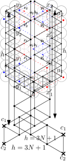
(a) $L(A)$, where the triangle $a_{i}x_{i}x^{\prime}_{i}$ exists if and only if $i\in A$

(b) $R(B)$, where the triangle $b_{i}y_{i}y^{\prime}_{i}$ exists if and only if $i\in B$

(c) $g(L(A),R(B)$ obtained by identifying $c_{1}$ and $c_{2}$. Grey circles show the only possible position for a penny representation of the graph, with a collision between $a_{i}$ and $b_{i}$.

Figure 2. Construction of $L,R$ and $g$ for penny graphs in the case where $N=2$, with $A,B\subseteq\{1,\ldots,N\}$. Color red highlights vertices and edges that depend on the choice of $A$, and color blue highlights vertices and edges that depend on the choice of $B$.

From Theorems 5.1 and 4.2, together with Corollary 3.2, we immediately deduce the following.

Theorem 5.2.

The local complexity of the class of penny graphs is $\Theta(n)$.

The exact same construction in the proof of Theorem 5.1 can be used to show the following. Indeed, conditions (i) and (ii) of the definition of disjointness-expressing trivially hold (as we consider the same graph) and the same rigidity arguments show that $g(L(A),R(B))$ is a unit-distance graph if and only if $A$ and $B$ are disjoint.

Theorem 5.3.

The class of unit-distance graphs is $(6,1)$-disjointness-expressing.

As above we have the following consequence.

Theorem 5.4.

The local complexity of the class of unit-distance graphs is $\Omega(n)$.

We observe that rigidity properties similar to those used in the proof of Theorem 5.1 can be obtained in higher dimension $d\geq 3$ with a very similar construction. This suggests that via a very similar proof one can obtain a linear lower bound on the local complexity of contact graphs of balls and unit-distance graphs in dimension $d$, for any $d\geq 3$.

5.2. Subgraphs of the square grid

(a) $L(A)$, where the block $D^{L}_{i}$ (4 vertices, 6 edges) exists if and only if $i\in A$

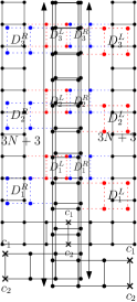
(b) $R(B)$, where the block $D^{R}_{i}$ (4 vertices, 6 edges) exists if and only if $i\in B$

(c) $g(L(A),R(B)$ obtained by identifying $c_{1}$ and $c_{2}$.

Figure 3. Construction of $L,R$ and $g$ for subgraphs of the square grid in the case where $N=3$, with $A,B\subseteq\{1,\ldots,N\}$. Color red highlights vertices and edges that depend on the choice of $A$, and color blue highlights vertices and edges that depend on the choice of $B$.

Theorem 5.5.

The class of subgraphs of the square grid is $(6,1)$-disjointness-expressing.

Proof.

The construction is described in Figure 3, and is very similar to the one used for penny graphs in Theorem 5.1. We denote by $D^{L}_{i}$ a left-truncated domino containing 4 vertices and 6 edges, attaching to 2 existing vertices on the left, as shown by one red block on the figure. We add such a subgraph $D^{L}_{i}$ in $L(A)$ if and only if $i$ belongs to $A$. Similarly we define a right-truncated domino $D^{R}_{i}$ containing 4 vertices and 6 edges, attaching to 2 existing vertices on the right, as shown by one blue block on the figure, and $D^{R}_{i}$ is present in $R(B)$ if and only if $i$ belongs to $B$. The set $S=\{c_{1},c_{2}\}$ has size 2 and we can observe that the subgraph induced by the neighborhood of $S$ in $g(L(A),R(B))$ is independent from the choice of $A$ and $B$ and has size at most 6, which fulfills Condition (ii) of disjointness-expressing. Moreover the size of $g(L(A),R(B))$ is at most $20N+18$, satisfying Condition (i) with $\varepsilon=1$. Finally, we claim that if $g(L(A),R(B))$ is a subgraph of the square grid, the blocks $D^{L}_{i}$ and $D^{R}_{i}$ cannot both exist because there is not enough space in the grid to fit two different vertices at their extremities, in a sense that we explain now. Observe that $g(L(A),R(B))$ can be constructed by gluing $C_{4}$’s along their edges. As every edge of the square grid is shared by exactly two $C_{4}$’s, as soon as we embed one $C_{4}$ of $g(L(A),R(B))$ as an induced subgraph of the square grid, there is at most one way to extend this to an embedding of $g(L(A),R(B))$ as an induced subgraph of the square grid. If both $D^{L}_{i}$ and $D^{R}_{i}$ exist in $g(L(A),R(B))$ and this graph is an induced subgraph of the grid, the aforementioned rigidity property implies that two vertices of the grid belong to both of the truncated dominos, which is impossible since these subgraphs are disjoint in $g(L(A),R(B))$. So in this case, $g(L(A),R(B))$ is not a subgraph of the grid. Conversely it is easy to check that when $A$ and $B$ are disjoint, $g(L(A),R(B))$ is indeed an induced subgraph of the grid. This shows Condition (iii). ∎

From the proof above, we deduce the following result for induced subgraphs of the square grid.

Corollary 5.6.

The class of induced subgraphs of the square grid is $(6,1)$-disjointness-expressing.

Proof.

As noticed in the proof of Theorem 5.5, the graph $g(L(A),R(B))$ is an induced subgraph of the square grid whenever $A\cap B=\emptyset$. Therefore by Remark 4.3, Item 2, the class of induced subgraphs of the square grid is disjointness-expressing with the same parameters as subgraphs of the square grids. ∎

From Theorem 5.5, Corollary 5.6, and Theorem 4.2, together with Corollary 3.2, we immediately deduce the following.

Theorem 5.7.

The local complexity of the class of (induced) subgraphs of the square grid is $\Theta(n)$.

Using similar techniques, we can prove that the same holds for grids in any fixed dimension $d\geq 2$.

5.3. 1-planar graphs

Theorem 5.8.

The class of 1-planar graphs is $(20,1)$-disjointness-expressing.

Proof.

Figure 4 illustrates the graph used in the proof. That this is the only possible $1$-planar embedding of this graph follows from a result of [18] (about the outer ring of vertices, which is $C_{2N+6}\boxtimes P_{4}$). On the one hand, $L(A)$ has $2N+8$ vertices, including the special vertices $c_{1},\ldots,c_{4}$, and the dotted edge $a_{i}a^{\prime}_{i}$ exists if and only if $i\in A$. On the other hand, $R(B)$ has $10N+25$ vertices, including the same four special vertices $c_{1},\ldots,c_{4}$, and the dotted edge $b_{i}b_{i+1}$ exists if and only if $i\in B$. If $A$ and $B$ are disjoint then the graph $g(L(A),R(B))$ is clearly 1-planar. We now prove that the converse also holds. Consider some $i\in A\cap B$ and assume for the sake of contradiction that $g(L(A),R(B))$ is 1-planar. Then the edge $a_{i}a^{\prime}_{i}$ must cross two edges: $b_{i}b_{i+1}$, and one edge incident to the degree-2 common neighbor of $b_{i}$ and $b_{i+1}$, which is a contradiction. Hence this graph is $1$-planar if and only if $A\cap B=\emptyset$. This proves Condition (iii) of disjointness-expressing. Condition (i) is satisfied with $\varepsilon=1$ because $g(L(A),R(B))$ has order $12N+29$. Finally regarding Condition (ii), by construction the closed neighborhood of $S=\{c_{1},c_{2},c_{3},c_{4}\}$ in $g(L(A),R(B))$ is independent of the choice of $A$ and $B$ and has size $s=20$.

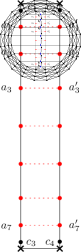
(a) $L(A)$ where $a_{i}a^{\prime}_{i}\in E$ iff $i\in A$

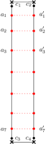
(b) $R(B)$ where $b_{i}b_{i+1}\in E$ iff $i\in B$

(c) $g(L(A),R(B))$ obtained by identifying $c_{1},\ldots,c_{4}$

Figure 4. The construction of $L$, $R$ and $g$ for 1-planar graphs in the case where $N=7$, with $A,B\subseteq\{1,\ldots,N\}$. Color red highlights edges that depend on the choice of $A$, and color blue highlights edges that depend on the choice of $B$.

∎

It seems plausible that a generalization of the result of Theorem 5.8 to $k$-planar graphs can be obtained from the same construction by adding for each edge $uv$ a set of $k-1$ new degree-2 vertices adjacent to both $u$ and $v$.

From Theorems 5.8 and 4.2, together with Corollary 3.2, we immediately deduce the following.

Theorem 5.9.

The local complexity of the class of 1-planar graphs is $\Theta(n)$.

6. Unit-square graphs

Given a set $S$ of points in the plane, the unit-square graph associated to $S$ is the graph with vertex set $S$ in which two points are adjacent if and only if their $\ell_{\infty}$-distance is at most 1. We say that a graph is a unit-square graph if it is the unit-square graph associated to some set of points in the plane. Equivalently, unit-square graphs can be defined as follows: the vertices correspond to axis-parallel squares of side length 1 (or any fixed value $r$, the same for all squares), and two vertices are adjacent if and only if the corresponding squares intersect. The equivalence can be seen by associating to each square its center, and to each point the axis-parallel square of side 1 centered in this point. It will sometimes be convenient to consider the two (equivalent) definitions at once, as each of them has some useful properties.

We say that a unit-square graph $G$ is embedded in the plane if it is given by a fixed set $S$ of points as above (or equivalently a set of unit-squares). The embedding is then referred to as a unit-square embedding of $G$. Recall that by Proposition 2.1, any triangle-free unit-square graph $G$ embedded in the plane gives rise to a planar graph embedding of $G$. Note that some planar graph embeddings of $G$ do not correspond to any unit-square embedding (even up to homeomorphism).

We start with some simple observations about triangle-free unit-square graphs.

Observation 6.1.

Let $G$ be a triangle-free unit-square graph associated to a set $\mathcal{S}=(S_{v})_{v\in V(G)}$ of unit-squares. Then $G$ has maximum degree 4, and for each vertex $v$ of degree 4 in $G$, each of the four corners of $S_{v}$ is contained in the square of a different neighbor of $v$ (and $S_{v}$ contains the opposite corner of each of the squares of the neighbors of $v$).

Given a triangle-free unit-square graph $G$ associated to a set $\mathcal{S}=(S_{v})_{v\in V(G)}$ of unit-squares, and a vertex $v$, we denote by $n_{00}(v)$, $n_{10}(v)$, $n_{01}(v)$ and $n_{11}(v)$ the neighbors of $v$ whose squares intersect the bottom-left, bottom-right, top-left, and top-right corner of the square of $v$, respectively (see Figure 5). In general these vertices might coincide, but since $G$ is triangle-free there is at most one neighbor of each type. By Observation 6.1, when $v$ has degree 4, all vertices $n_{00}(v)$, $n_{10}(v)$, $n_{01}(v)$ and $n_{11}(v)$ exist and are distinct.

Figure 5. A vertex of degree 4 in a triangle-free unit-square graph.

For each unit-square graph $G$ embedded in the plane and each vertex $u$ in $G$, we denote by $x(u)$ and $y(u)$ the $x$- and $y$-coordinates of the center of the square associated to $u$ in the embedding.

Observation 6.2.

Let $G$ be a triangle-free unit-square graph embedded in the plane, and let $u,v,w$ be three distinct vertices.

• If $v=n_{11}(u)$ and $w=n_{10}(u)$, then $y(v)>y(w)+1$;

• If $v=n_{01}(u)$ and $w=n_{00}(u)$, then $y(v)>y(w)+1$;

• If $v=n_{10}(u)$ and $w=n_{00}(u)$, then $x(v)>x(w)+1$;

• If $v=n_{11}(u)$ and $w=n_{01}(u)$, then $x(v)>x(w)+1$.

Figure 6. A horizontal prop of length 4 (left), a vertical prop of length 2 (right), and the associated planar graph embeddings (which are unique up to homeomorphism, by Observation 6.4).

Let $G$ be a triangle-free unit-square graph embedded in the plane. For $n\geq 1$, a horizontal prop of length $n$ in $G$ is a sequence of distinct vertices $(u_{i})_{0\leq i\leq n}$, $(v_{i})_{0\leq i\leq n-1}$, and $(w_{i})_{0\leq i\leq n-1}$, such that the following holds: for each $0\leq i\leq n-1$, $v_{i}=n_{11}(u_{i})$, $w_{i}=n_{10}(u_{i})$, and $u_{i+1}=n_{10}(v_{i})=n_{11}(w_{i})$. Similarly, a vertical prop of length $n$ in $G$ is a sequence of distinct vertices $(u_{i})_{0\leq i\leq n}$, $(v_{i})_{0\leq i\leq n-1}$, and $(w_{i})_{0\leq i\leq n-1}$, such that the following holds: for each $0\leq i\leq n-1$, $v_{i}=n_{10}(u_{i})$, $w_{i}=n_{00}(u_{i})$, and $u_{i+1}=n_{00}(v_{i})=n_{10}(w_{i})$ (see Figure 6). The vertices $u_{0}$ and $u_{n}$ are respectively said to be the starting and ending vertex of the (horizontal or vertical) prop.

We easily deduce the following from Observation 6.2.

Observation 6.3.

Let $G$ be a triangle-free unit-square graph embedded in the plane, and let $u_{0}$ and $u_{n}$ be the starting and ending vertices of a prop of length $n$ in $G$. If the prop is horizontal, then $x(u_{n})>x(u_{0})+n$. If the prop is vertical, then $y(u_{0})>y(u_{n})+n$.

Let $\mathrm{Pr}_{n}$ denote the graph induced by a (vertical or horizontal) prop of length $n$. That is, $\mathrm{Pr}_{n}$ can be obtained from $n$ disjoint 4-cycles $u_{i}v_{i}u_{i}^{\prime}w_{i}$ ($0\leq i\leq n-1)$ by identifying $u_{i}^{\prime}$ with $u_{i+1}$, for each $0\leq i\leq n-2$. Then $\mathrm{Pr}_{n}$ has $3n+1$ vertices. Consider any fixed embedding of $\mathrm{Pr}_{n}$ in the plane as a unit-square graph. Since $\mathrm{Pr}_{n}$ is triangle-free, this unit-square embedding of $\mathrm{Pr}_{n}$ also gives a planar embedding of $\mathrm{Pr}_{n}$ (with the same circular order of neighbors around each vertex), see Proposition 2.1. There are multiple non-equivalent planar embeddings of $\mathrm{Pr}_{n}$, however a simple area computation shows that in any planar graph embedding coming from a unit-square embedding of $\mathrm{Pr}_{n}$ each 4-cycle of $\mathrm{Pr}_{n}$ is a face, distinct from the outerface, so up to homeomorphism the resulting planar embedding is unique. This implies the following.

Observation 6.4.

Let $G$ be a triangle-free unit-square graph embedded in the plane and let $H$ be a subgraph of $G$ that is isomorphic to $\mathrm{Pr}_{n}$. Then $H$ is a vertical or horizontal prop of length $n$ in $G$.

We are now ready to prove the main result of this section.

Theorem 6.5.

The class of triangle-free unit-square graphs is $(6,1)$-disjointness-expressing.

Proof.

Consider the graph $G_{k}$ depicted in Figure 7, where $k\geq 1$ is an integer. It consists of:

• a cycle $C$ of length $16k+16$, depicted with bold black edges in Figure 7;

• a copy of $\mathrm{Pr}_{8k+6}$ with endpoints $v_{1},v_{3}\in C$ with $v_{1}$ and $v_{3}$ antipodal on $C$;

• another copy of $\mathrm{Pr}_{8k+6}$ with endpoints $v_{2},v_{4}\in C$, such that $v_{2}$ and $v_{4}$ are antipodal on $C$ and, for any $1\leq i\leq 4$, $v_{i}$ and $v_{i+1}$ are at distance $4k+4$ on $C$ (where indices are taken modulo 4 plus 1). Moreover the two props intersect in their middle, forming a star on 5 vertices (depicted in bold red edges in Figure 7);

• on the subpath of $C$ of length $4k+4$ between $v_{1}$ and $v_{2}$, there exists a unique vertex set $I$ of size $k$ in which all vertices are at distance at least 4 from $v_{1}$ and $v_{2}$ on $C$, and any two vertices of $I$ are at distance at least 4 on $C$. For each vertex $v\in I$, we create two copies of a 3 by 3 grid and add an edge between $v$ and a vertex of degree 3 in each of the two grids. The $2k$ copies of the grid are denoted by $H_{1},H_{1}^{\prime},\ldots,H_{k},H_{k}^{\prime}$ in order from $v_{1}$ and $v_{2}$.

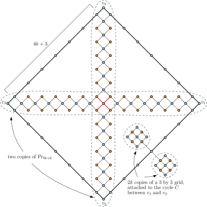
Figure 7. The graph $G_{k}$ for $k=1$.

Note that $G_{k}$ contains exactly $(16k+16)+(48k+21)+18k=82k+37=O(k)$ vertices. Intuitively, up to a few technical vertex additions, two copies of $G_{k}$ will be used as $L(X)$ and $R(X)$ respectively, for $X\subseteq\{1,\ldots,k\}$, where $H_{i}$ and $H_{i}^{\prime}$ will be removed if $i\notin X$. Before we explain how the two copies of $G_{k}$ are glued together, we analyze the properties of $G_{k}$. First of all, $G_{k}$ can easily be realized as a unit-square graph (see the top-left part of Figure 8, where colored vertices are represented by a square of the same color). We note that we have only represented $G_{1}$ so it is not immediately clear that several copies $H_{1},H_{1}^{\prime},\ldots,H_{k},H_{k}^{\prime}$ can fit together without overlapping. This simply follows from the fact that consecutive copies indexed $i,i+1$ of the 3 by 3 grid are attached to vertices lying at distance 4 on $C$.

Fix any embedding of $G_{k}$ as a unit-square graph. For each vertex $v\in V(G)$, we also write $v$ for the center of the square associated to $v$ in this embedding. Writing $d_{\infty}$ for the $\ell_{\infty}$-distance and $d_{G}$ for the distance in $G$, it follows from the definition of a unit-square graph that for any two vertices $u,v\in V(G)$, $d_{\infty}(u,v)\leq d_{G}(u,v)$. In particular $d_{\infty}(v_{i},v_{i+1})\leq 4k+4$ and $d_{\infty}(v_{i},v_{i+2})\leq 8k+8$ for any $1\leq i\leq 4$ (with indices taken modulo 4 plus 1). By Observation 6.4 and up to rotation and reflection, we can assume that the prop with endpoints $v_{1}$ and $v_{3}$ is a horizontal prop starting in $v_{3}$ and ending in $v_{1}$, and that the second prop is a vertical prop starting in $v_{4}$ and ending in $v_{2}$, precisely as in Figure 7.

By Observation 6.3, $d_{\infty}(v_{1},v_{3})>8k+6$ and $d_{\infty}(v_{2},v_{4})>8k+6$. As $d_{\infty}(v_{i},v_{i+1})\leq 4k+4$ for any $1\leq i\leq 4$, this implies (by the triangle inequality) that $d_{\infty}(v_{i},v_{i+1})>4k+2$ for any such $i$ (with indices taken modulo 4 plus 1). Hence, we have proved that $4k+2<d_{\infty}(v_{1},v_{2})\leq 4k+4$. Using Observation 6.3, this implies that

$$4k+2<|x(v_{1})-x(v_{2})|\leq 4k+4\text{ and }4k+2<|y(v_{1})-y(v_{2})|\leq 4k+4,$$

where $x(\cdot)$ and $y(\cdot)$ denote the $x$- and $y$-coordinates of the points as before. Let us denote by $u_{1},u_{2},\ldots,u_{4k+5}$ the vertices on the subpath $P$ of $C$ of length $4k+4$ between $v_{1}$ and $v_{2}$ (with $u_{1}=v_{1}$ and $u_{4k+5}=v_{2}$). The previous result implies that for any $1\leq i\leq j\leq 4k+5$,

$$j-i-2<|x(u_{i})-x(u_{j})|\leq j-i\text{ and }j-i-2<|y(u_{i})-y(u_{j})|\leq j-i.$$

In particular, if we translate and rotate the vertices of the embedding of $G_{k}$ such that $v_{1}$ lies at coordinates $(0,0)$ and $v_{2}$ lies at $\ell_{\infty}$-distance at most 2 from $(4k+4,4k+4)$, then for any $1\leq i\leq 4k+5$, $u_{i}$ lies in the square with corners $(i-3,i-3)$ and $(i-1,i-1)$. We call this property the almost-perfect rigidity of $G_{k}$.

The paragraph above also shows that if we only consider the subgraph of $G_{k}$ induced by the vertices of $C$ and the vertices of the two props, in any unit-square embedding of this graph the outerface of the embedding must be bounded by $C$ (otherwise one of the subpaths dividing $C$ would have to be much longer than what is possible). By Observation 6.1, for each vertex $v\in I$, one of the copies of the 3 by 3 grid attached to $v$ lies inside $C$ while the other must lie outside $C$ (it can be checked that the two copies cannot intersect two adjacent corners of a given square, since otherwise the two copies would overlap). In conclusion, the planar graph embedding corresponding to a unit-square embedding of $G_{k}$ is unique (up to homeomorphism and reflection), and corresponds precisely to the planar embedding depicted in Figure 7.

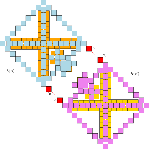
Figure 8. $L(A)$ and $R(B)$ in the proof of Theorem 6.5, when $k=1$ and $A=B=\{1\}$.

We now define $G_{k}^{\prime}$ as the graph obtained from $G_{k}$ by adding a vertex $c_{1}$ adjacent to $v_{1}$ and a vertex $c_{2}$ adjacent to $v_{2}$, and setting $S=\{c_{1},c_{2}\}$ as a set of special vertices. For every $X\subseteq\{1,\ldots,N\}$, we set $L(X)$ and $R(X)$ as $G_{N}^{\prime}$, in which we delete all copies $H_{i}$ and $H_{i}^{\prime}$ ($1\leq i\leq N$) such that $i\not\in X$. For $A,B\subseteq\{1,\ldots,N\}$, $g(L(A),R(B))$ is obtained from $L(A)$ and $R(B)$ by gluing them along their special vertices. This is illustrated in Figure 8, where $L(A)$ and $R(B)$ have been drawn disjointly, for the sake of clarity, and in Figure 9, where only the interface between $L(A)$ and $R(B)$ was represented. As illustrated in Figure 9 (left), it follows from the almost-perfect rigidity of $G_{k}$ that if $H_{i}$ and $H_{i}^{\prime}$ are present both in $L(A)$ and $R(B)$, then some square of $H_{i}$ or $H_{i}^{\prime}$ in $L(A)$ must intersect some square of $H_{i}$ or $H_{i}^{\prime}$ in $R(B)$, which is a contradiction as there are no edges between these copies in $g(L(A),R(B))$.

The results obtained above show that for any $A,B\subseteq\{1,\ldots,N\}$, $g(L(A),R(B))$ is triangle-free, and it a unit-square graph if and only if $A$ and $B$ are disjoint. As $G_{N}^{\prime}$ and $G_{N}$ have $O(N)$ vertices and the closed neighborhood of $S$ is independent of $A$ and $B$ and has size 6, the class of triangle-free unit-square graphs is $(6,1)$-disjointness-expressing. ∎

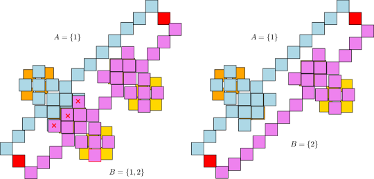
Figure 9. The interface between $L(A)$ and $R(B)$ when $k=2$ and $A=\{1\}$ and $B=\{1,2\}$ (left), and when $A=\{1\}$ and $B=\{2\}$ (right). The red crosses indicate the squares of $H_{i}$ or $H_{i}^{\prime}$ in $L(A)$ that intersect those of $H_{i}$ or $H_{i}^{\prime}$ in $R(B)$.

In the proof of Theorem 6.5 we have shown that when $A$ and $B$ are disjoint, then the resulting graph $g(L(A),R(B))$ is not a unit-square graph. Using Remark 4.3, we obtain the following as a direct consequence.

Corollary 6.6.

The class of unit-square graphs is $(6,1)$-disjointness-expressing.

Using Theorem 4.2, together with Corollaries 3.2 and 3.3, we immediately deduce the following.

Theorem 6.7.

The local complexity of the class of triangle-free unit-square graphs is $\Theta(n)$, and the local complexity of the class of unit-square graphs is $\Omega(n)$ and $O(n\log n)$.

We note that the proof approach of Theorem 6.5 naturally extends to higher dimension.

7. Unit-disk graphs

7.1. Definition

The Euclidean distance between two points $x$ and $y$ in the plane is denoted by $d_{2}(x,y)$, to avoid any confusion with the $\ell_{\infty}$-distance $d_{\infty}$ considered in the previous section, and the distance $d_{G}(u,v)$ between two vertices $u$ and $v$ in a graph $G$. Given a set $S$ of points in the plane, the unit-disk graph associated to $S$ is the graph with vertex set $S$ in which two points are adjacent if and only if their Euclidean distance is at most 1. We say that a graph is a unit-disk graph if it is the unit-disk graph associated to some set of points in the plane. Equivalently, unit-disk graphs can be defined as follows: the vertices correspond to disks of radius $\tfrac{1}{2}$ (or any fixed radius $r$, the same for all disks), and two vertices are adjacent if and only if the corresponding disks intersect. In particular, penny graphs are unit-disk graphs.

7.2. Discussion

We would like to prove a variant of Theorem 6.5 for unit-disk graphs, but there are two major obstacles. The first is that there does not seem to be a simple equivalent of a horizontal or vertical prop in unit-disk graphs, that is a unit-disk graph with $O(n)$ vertices with two specified vertices that are at Euclidean distance at least $n$ in any unit-disk embedding. Our construction of such a graph will be significantly more involved. The second obstacle comes from Pythagora’s theorem: In the unit-square case, if we consider a path $P$ of length $n+O(1)$ between two vertices $u,v$ embedded in the plane such that their $x$- and $y$-coordinates both differ by exactly $n$, then in any unit-square embedding of $P$, the vertices of $P$ deviate by at most a constant from the line segment $[u,v]$ between $u$ and $v$. This is what we used in the proof of the previous section to make sure that $L(A)$ and $R(B)$ (intuitively, Alice’s and Bob’s parts) are so close that the $i$-th gadget cannot exist both on $L(A)$ and $R(B)$ simultaneously when $i\in A\cap B$ (i.e., Alice’s and Bob’s subsets must be disjoint for the graph to be in the class). However, Pythagora’s theorem implies that in the Euclidean case, when the Euclidean distance between $u$ and $v$ is equal to $n$, the vertices of $P$ can deviate by $\Theta(\sqrt{n})$ from the line segment $[u,v]$, which is too much for our purpose (we need a constant deviation). So we need different ideas to make sure the gadgets are embedded sufficiently close from each other.

Figure 10. A summary of the construction used in the proof of Theorem 7.16.

A summary of our construction is depicted in Figure 10. We now describe the different steps of the construction in details. In order to not disrupt the flow of reading, the technical proofs from this section have been deferred to the appendix (with the same numbering). This is marked by a symbol ✂ which links to the relevant appendix section.

7.3. Stripes

For $k,\delta>0$, a triangle in the plane is said to be $(k,\delta)$-almost-equilateral if all sides have length at least $k-\delta$ and at most $k+\delta$. By the law of cosines and the approximation $\arccos(1/2-x)=\pi/3+O(x)$ as $x\to 0$, we have the following.

Observation 7.1.

All angles in a $(k,\delta)$-almost-equilateral triangle with $k\gg\delta$ are between $\tfrac{\pi}{3}-O(\delta/k)$ and $\tfrac{\pi}{3}+O(\delta/k)$.

For $\ell\geq 0$, the stripe $S_{\ell}$ with vertex set $u_{0},v_{0},\ldots,u_{\ell},v_{\ell}$ is the graph defined as follows: $u_{0}v_{0}$ is an edge and for any $i\geq 1$, $u_{i}$ is adjacent to $u_{i-1}$ and $v_{i-1}$, and $v_{i}$ is adjacent to $v_{i-1}$ and $u_{i}$. Note that this graph can also be obtained from a sequence of triangles by gluing any two consecutive triangles on one of their edges. The vertices $u_{0}$ and $v_{\ell}$ are called the ends of the stripe $S_{\ell}$.

We say that the stripe $S_{\ell}$ has a $(k,\delta)$-almost-equilateral embedding in the plane if the vertices $u_{0},v_{0},\ldots,u_{\ell},v_{\ell}$ are embedded in the plane in such way that all triangles of $S_{\ell}$ are $(k,\delta)$-almost-equilateral (see Figure 11 for an illustration where $k\gg\delta$).

Figure 11. A $(k,\delta)$-almost-equilateral embedding of a stripe, where the Euclidean distance between the ends is minimized.

We show that in a $(k,\delta)$-almost-equilateral embedding of the stripe that minimizes the Euclidean distance between its ends, the vertices of the stripe are close to a circular arc whose radius only depends on $(k,\delta)$. The Menger curvature of a triple of points $a,b,c$ is the reciprocal of the radius of the circle that passes through $a$, $b$, and $c$.

Lemma 7.2 (✂).

For every $k$ and $\delta=o(k)$, there are $\rho=\rho(k,\delta)$ and $\rho^{\prime}=\rho^{\prime}(k,\delta)$ such that for any $\ell$, the following holds. Consider a $(k,\delta)$-almost-equilateral embedding of the stripe $S_{\ell}$ that minimizes $d_{2}(u_{0},v_{\ell})$. Then (up to changing all $u_{i}$’s by $v_{i}$’s and vice versa), all triples $v_{i-1},v_{i},v_{i+1}$ have the same Menger curvature $1/\rho$, and all triples $u_{i-1},u_{i},u_{i+1}$ have the same Menger curvature $1/\rho^{\prime}$. In particular all vertices $v_{i}$ lie on some circular arc of radius $\rho$, and all vertices $u_{i}$ lie on some circular arc of radius $\rho^{\prime}$.

By Observation 7.1, the maximum angle between the lines $u_{i}v_{i}$ and $u_{i+1}v_{i+1}$ is of order $O(\delta/k)$. Hence, there exists a constant $\alpha$ (independent of $k$ and $\delta$) such that if $\ell=\alpha k/\delta$, the maximum angle between $u_{0}v_{0}$ and $u_{\ell}v_{\ell}$ in any $(k,\delta)$-almost-equilateral embedding is close to $\pi$. In this case, by Lemma 7.2 the minimum (Euclidean) distance $m$ between $u_{0}$ and $v_{\ell}$ in any $(k,\delta)$-almost-equilateral embedding is of order $\Theta(k/\delta\cdot k)=\Theta(k^{2}/\delta)$. Moreover, any $(k,\delta)$-almost-equilateral embedding of $S_{\ell}$ realizing this minimum $m$ is close to some semicircle with endpoints $u_{0}$ and $v_{\ell}$, in the sense that all the vertices of $S_{\ell}$ lie at distance $O(k)$ from the semicircle (see Figure 11). We will need a looser version of this observation in the slightly weaker setting where $d_{2}(u_{0},v_{\ell})\leq m+1$, instead of $d_{2}(u_{0},v_{\ell})=m$.

Lemma 7.3 (✂).

Let $k\gg\delta$ and $\ell=\lceil\alpha k/\delta\rceil$ as above, and let $m=\Theta(k^{2}/\delta)$ be the minimum Euclidean distance between $u_{0}$ and $v_{\ell}$ in any $(k,\delta)$-almost-equilateral embedding of $S_{\ell}$. Consider a $(k,\delta)$-almost-equilateral embedding of $S_{\ell}$ where $d_{2}(u_{0},v_{\ell})\leq m+1$. Let $c$ be the midpoint of the segment $[u_{0},v_{\ell}]$. Then no vertex of the stripe $S_{\ell}$ is contained in the disk of center $c$ and radius $m/2-O(k)$, and all vertices of the stripe $S_{\ell}$ are contained in a disk of center $c$ and radius $O(m)=O(k^{2}/\delta)$.

7.4. Quasi-rigid graphs

Our next goal is to construct a sequence of unit-disk graphs $T_{n}$ on $O(n^{2})$ vertices, with two vertices $u$ and $v$ such that in any unit-disk representation of $T_{n}$, $d_{2}(u,v)=\Omega(n)$.

We define $T_{n}$ as follows. We consider two adjacent vertices $u,v$ of the infinite square grid and define $X$ as the set of vertices at distance at most $2n+1$ from $u$ or $v$ in the square grid, and $Y\subseteq X$ as the set of vertices at distance exactly $2n+1$ from $u$ or $v$. Note that $|X|=2(2n+2)^{2}=8(n+1)^{2}$ and $|Y|=8n+6$. The vertices of $Y$ are denoted by $y_{1},\ldots,y_{8n+6}$. The graph $T_{n}$ is obtained from the subgraph of the square grid induced by $X$ by adding, for each vertex $y_{i}$ of $Y\subseteq X$, a vertex $c_{i}$ adjacent to $y_{i}$. We finally add edges to form a cycle $C$ containing all vertices $c_{i}$ in order, together with 10 new vertices (2 or 3 at each corner, see Figure 12). The resulting cycle $C$ has length $8n+16$. Note that the resulting graph $T_{n}$ contains $8n^{2}+24n+24=O(n^{2})$ vertices and is a planar triangle-free unit-disk graph (see Figure 12). A simple area computation shows that in any unit-disk embedding of $T_{n}$, $C$ bounds the outerface of the corresponding planar graph embedding (by the arguments of Section 2.2 there is a unique planar graph embedding in the sphere, and as all faces except $C$ have size at most 8, $C$ must be the outerface).

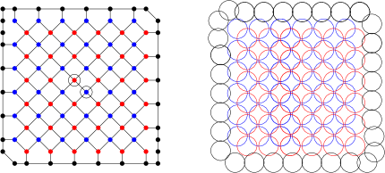
Figure 12. The graph $T_{n}$ with $n=2$ (left), with the central vertices $u$ and $v$ circled ; and a unit-disk embedding of $T_{n}$ (right).

Lemma 7.4 (✂).

Let $c$ and $c^{\prime}$ be two antipodal vertices on the cycle $C$ in $T_{n}$. In any unit-disk embedding of $T_{n}$, $d_{2}(c,c^{\prime})\geq\left(\pi\sqrt{2}-4\right)n-O(\sqrt{n})=\Omega(n)$.

Let $f(n)$ be the infimum Euclidean distance between two antipodal vertices $c$ and $c^{\prime}$ of the cycle $C$ in a unit-disk embedding of $T_{n}$. By Lemma 7.4, $f(n)=\Omega(n)$. Since $C$ has length $O(n)$, it follows that $f(n)=\Theta(n)$. Assume for simplicity that the infimum $f(n)$ is a minimum (otherwise we work with a sequence of unit-disk embeddings such that the Euclidean distance between $c$ and $c^{\prime}$ tends to $f(n)$). Let $Z_{n}$ be the point set of a unit-disk embedding of $T_{n}$ in which $d_{2}(c,c^{\prime})=f(n)$. Add $\lceil f(n)\rceil-1$ points, evenly spaced on the line-segment $[c,c^{\prime}]$ (note that together with $c$ and $c^{\prime}$, any two consecutive points on $[c,c^{\prime}]$ lie at distance at most 1 apart). Let $Z_{n}^{\prime}$ denote the resulting point set and $T_{n}^{\prime}$ be the resulting unit-disk graph. Note that $T_{n}^{\prime}$ has $O(n^{2})$ vertices and in any unit-disk graph embedding of $T_{n}^{\prime}$, $f(n)\leq d_{2}(c,c^{\prime})\leq f(n)+1$, with $f(n)=\Omega(n)$.

We say that an infinite family of unit-disk graphs $\mathcal{T}$ is quasi-rigid with density $g$ if for arbitrarily large $k$ there is a graph $G\in\mathcal{T}$ with at most $g(k)$ vertices, and two specific vertices $x$ and $y$ in $G$ such that in any unit-disk embedding of $G$, $k\leq d_{2}(x,y)\leq k+1$. Using this terminology, the family $\mathcal{T}^{2}=(T_{n}^{\prime})_{n\geq 1}$ is quasi-rigid with density $O(k^{2})$. We will now see how to construct increasingly sparser quasi-rigid classes, starting with $\mathcal{T}^{2}$ and using stripes.

Figure 13. Copies of a point set are glued along some stripe.

Assume we have found a family $\mathcal{T}^{1+c}$ which is quasi-rigid with density $g(k)=O(k^{1+c})$, for some $c\geq 0$. Take some graph $G\in\mathcal{T}^{1+c}$ with $g(k)$ vertices and that has two vertices $x$ and $y$ such that in any unit-disk embedding of $G$, $k\leq d_{2}(x,y)\leq k+1$. Let $X$ be the point set associated to some unit-disk embedding of $G$, and let $d:=d_{2}(x,y)$ in this point set ($k\leq d\leq k+1$). Consider a $(d,0)$-almost equilateral embedding of a stripe $S_{\ell}$ (for some integer $\ell\geq 0$ whose value will be fixed later), and for each edge $uv$ in $S_{\ell}$, add an isometric copy of $X$ in which $x$ is identified with $u$ and $y$ is identified with $v$ (by definition of $X$ we can always find such an isometric copy of $X$). See Figure 13 for an illustration. We denote by $X^{(\ell)}$ the resulting point set, and by $G^{(\ell)}$ the resulting unit-disk graph. Note that the different copies of $X$ interact and thus $G^{(\ell)}$ contains more edges than the unions of copies of $G$. Fix any unit-disk embedding of $G^{(\ell)}$, and consider the points corresponding to $x$ and $y$ in each of the copies of $G$ in $G^{(\ell)}$. By the properties of $G$, the union of all these points form a $(d,1)$-almost equilateral embedding of a stripe $S_{\ell}$. Let $a$ and $b$ be the ends of this stripe. By Lemma 7.3, there exists a constant $\alpha>0$ such that if we set $\ell=\lceil\alpha d\rceil=O(k)$, the following holds. Let $m$ be the minimum distance between $a$ and $b$ in any unit-disk embedding of $G^{(\ell)}$. Then $m=\Theta(d^{2})=\Theta(k^{2})$. As before we consider a point set realizing this distance and we add $\lceil m\rceil-1$ evenly spaced points on the segment $[a,b]$. We denote the resulting unit-disk graph by $H$ and we note that in any unit-disk graph embedding of $H$, $m\leq d_{2}(a,b)\leq m+1$. The point set $X^{(\ell)}$ has size at most $5\ell g(k)=O(k^{2+c})$ as there are $4\ell+1$ edges in $S_{\ell}$. We have added at most $m=O(d^{2})=O(k^{2})$ vertices to the graph, so $H$ has $O(k^{2+c})$ vertices. As $m=\Omega(k^{2})$, the family of all graphs $H$ created in this way is quasi-rigid with density $g^{\prime}(k)=O(k^{1+c/2})$.

By iterating this construction, starting with $\mathcal{T}^{2}$ and using Lemma 7.3, we obtain the following result. See Figure 10 for a depiction of the construction.

Observation 7.5.

For any $\varepsilon>0$ there is a family of unit-disk graphs which is quasi-rigid with density $O(k^{1+\varepsilon})$. More precisely, for any sufficiently large $k$ there is a unit-disk graph $G$ with $O(k^{1+\varepsilon})$ vertices with two vertices $a$ and $b$ such that in any unit-disk embedding of $G$, $k\leq d_{2}(a,b)\leq k+1$, and $a$ and $b$ are joined by a path $P$ of length at most $k+1$ such that at least $k/2$ consecutive vertices of $P$ lie at Euclidean distance at least $\Omega(k)$ from $G-P$.

7.5. Tied-arch bridges

In the previous subsection we have constructed unit-disk graphs with a pair of vertices $a,b$ whose possible Euclidean distance in any unit-disk embedding lies in some interval $\left[m,m+1\right]$. This is still too much for our purposes, because Pythagora’s theorem then implies that a path $P$ of length $\lceil m\rceil$ between $a$ and $b$ might deviate from the line-segment $[a,b]$ by $\Omega(m^{1/2})$, which prevents us from using arguments similar to unit-square case. We now explain how to obtain an even tighter path. The idea will be to cut $P$ into $\log m$ subpaths of nearly equal length, and join the endpoints of these subpaths to the rest of the graph, using some paths of minimum length. See Figure 15 for an illustration of this step of the proof. We will then argue that for any unit-disk embedding, at least one of these subpaths will be maximally tight (i.e., at constant distance from the line-segment joining its endpoints).

Figure 14. The setting of Lemma 7.6.

In this section, $x>0$ and $0\leq\delta\leq 1$ are real numbers, and whenever we use the $O(\cdot)$ notation, we implicitly assume that $x\to\infty$ (see for instance the terms $O(1/x)$ and $O(\sqrt{\delta/x})$ in the statement of the next lemma). Let $abc$ be a triangle such that $d_{2}(a,b)=x$ and $d_{2}(a,c)+d_{2}(b,c)=x+\delta$, with $|d_{2}(a,c)-d_{2}(b,c)|\leq 1$. Assume by symmetry that $d_{2}(a,c)\leq d_{2}(b,c)$. In particular $\tfrac{1}{2}(x+\delta-1)\leq d_{2}(a,c)\leq\tfrac{1}{2}(x+\delta)$ and $\tfrac{1}{2}(x+\delta)\leq d_{2}(b,c)\leq\tfrac{1}{2}(x+\delta+1)$. Let $c^{\prime}$ be a point such that $d_{2}(a,c^{\prime})\leq d_{2}(a,c)$, $d_{2}(b,c^{\prime})\leq d_{2}(b,c)$, and $d_{2}(c,c^{\prime})\leq\rho$, for some constant $\rho=O(1)$. See Figure 14 for an illustration.

Lemma 7.6 (✂).

$\min\{d_{2}(a,c)-d_{2}(a,c^{\prime}),d_{2}(b,c)-d_{2}(b,c^{\prime})\}\leq\rho\sqrt{2\delta/x}+O(1/x)=O(\sqrt{\delta/x})$.

Consider a graph $G_{0}$ given by Observation 7.5 with parameter $2k$. The unit-disk graph $G_{0}$ thus contains $O(k^{1+\varepsilon})$ vertices and has two vertices $u^{\prime}$ and $v^{\prime}$ such that in any unit-disk embedding $2k\leq d_{2}(u^{\prime},v^{\prime})\leq 2k+1$ and $u^{\prime}$ and $v^{\prime}$ are joined by a path $P^{\prime}$ of length less than $2k+1$.

For any unit-disk embedding of a unit-disk graph $G$ and for any $\delta>0$, we say that a path with endpoints $a$ and $b$ in $G$ is $\delta$-tight if the length of the path and the Euclidean distance between $a$ and $b$ differ by at most $\delta$. With this terminology, the path $P^{\prime}$ defined in the previous paragraph is 1-tight for any unit-disk embedding of $G_{0}$. Note that by the triangle inequality, any subpath of a $\delta$-tight path is also $\delta$-tight.

By the second part of Observation 7.5, $P^{\prime}$ has a subpath $P$ of length $k$ with endpoints $u$ and $v$ such that all vertices of $P$ lie at Euclidean distance at least $\Omega(k)$ from $G_{0}-P^{\prime}$ in any unit-disk embedding. It will be convenient to work with this subpath $P$ instead of $P^{\prime}$, as a large region around $P$ is free of any vertices of $G_{0}-P^{\prime}$. For any unit-disk embedding of $G_{0}$, since $P^{\prime}$ is 1-tight, $P$ is also 1-tight and thus $k\leq d_{2}(u,v)\leq k+1$.

We consider a vertex $w$ of $P$, which divides $P$ into two consecutive paths $P_{0}$ and $P_{1}$, whose lengths differ by at most 1. We consider a unit-disk embedding of $G_{0}$ and look at the perpendicular bisector of the line-segment $[u,v]$. By connectivity, this line intersects $G_{0}-P$. Let $z$ be the first vertex of $G_{0}-P$ whose unit-disk is intersected by this line (if several such vertices exist we pick one arbitrarily); by the properties above, $z$ lies at distance at least $\Omega(k)$ from $w$. As in the construction of quasi-rigid graphs above Observation 7.5, we consider a point set corresponding to a unit-disk embedding of $G_{0}$ where the Euclidean distance $m^{*}$ between $z$ and $w$ is minimized and add, along the segment $[zw]$, $\lceil m^{*}\rceil-1$ evenly spaced new points. Observe that in the resulting unit-disk graph $G_{1}$ the newly added vertices correspond to a path $Q$ of minimum length between $z$ and $w$ (and possibly some extra edges between this path and $V(G_{0})$). Therefore we have $m^{*}\leq d_{2}(z,w)\leq\lceil m^{*}\rceil$ in any unit-disk embedding of $G_{1}$. We iterate this procedure recursively on $P_{0}$ and $P_{1}$, creating 4 consecutive subpaths $P_{00},P_{01},P_{10},P_{11}$ of $P$, and two new paths $Q_{0}$ and $Q_{1}$ joining the new midpoints to $G-P$. More precisely, for any $i\geq 0$, consider a unit-disk embedding of $G_{i}$, and any subpath $P_{\mathbf{x}}$ of $P$ with $\mathbf{x}\in\{0,1\}^{i}$ in $G_{i}$. Let $a,b$ denote the endpoints of $P_{\mathbf{x}}$. Then in $G_{i+1}$, $P_{\mathbf{x}}$ is split between $P_{\mathbf{x}0}$ (with endpoints $a$ and $c^{\prime}$) and $P_{\mathbf{x}1}$ (with endpoints $c^{\prime}$ and $b$), where $c^{\prime}$ is a midpoint of $P_{\mathbf{x}}$, which is then joined (in the way described above) via some path $Q_{\mathbf{x}}$ of minimal length to some vertex $z$ of $G_{i}-P$ lying at distance at most $\tfrac{1}{2}$ from the perpendicular bisector of the line segment $[ab]$. Note that by construction $G_{i+1}$ is a unit-disk graph. See Figure 15 for a picture of $G_{3}$.

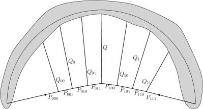
Figure 15. A tied-arch bridge.

Using the notation introduced in the previous paragraph, we obtain the following simple consequence of Lemma 7.6.

Corollary 7.7 (✂).

For any $\delta>0$ there exists $\gamma=O(\sqrt{\delta/d_{2}(a,b)})$ such that in any unit-disk embedding of $G_{i+1}$, if $P_{\mathbf{x}}$ is $\delta$-tight, then $P_{\mathbf{x}0}$ is $\gamma$-tight or $P_{\mathbf{x}1}$ is $\gamma$-tight.

Note that for any unit-disk embedding of $G_{i+1}$, the restriction of the embedding to $V(G_{i})\subset V(G_{i+1})$ is a unit-disk embedding of $G_{i}$ (the difference between $V(G_{i})$ and $V(G_{i+1})$ being the union of the newly added paths $Q_{\mathbf{x}}$). The following is proved by induction on $i\geq 0$.

Lemma 7.8 (✂).

In any unit-disk embedding of $G_{i}$, there is $\mathbf{x}\in\{0,1\}^{i}$ such that $P_{\mathbf{x}}$ is $O(2^{i}\cdot k^{2^{-i}-1})$-tight.

Consider a unit-disk embedding of a unit-disk graph $G$. For $\ell\geq 2$ and $\gamma\geq 0$, we say that a path $P=v_{1},\ldots,v_{\ell+1}$ of length $\ell$ in $G$ is $\gamma$-regular if the following holds: If we place $\ell+1$ evenly spaced points $u_{1},\ldots,u_{\ell+1}$ on the line-segment $[v_{1},v_{\ell+1}]$ with $u_{1}=v_{1}$ and $u_{\ell+1}=v_{\ell+1}$, then for any $1\leq i\leq\ell+1$, $d_{2}(u_{i},v_{i})\leq\gamma$. For $s\leq\ell+1$, we say that $P$ is $(\gamma,s)$-regular if the above holds for any $1\leq i\leq s$ (instead of $1\leq i\leq\ell+1$, so that $(\gamma,\ell+1)$-regular is the same as $\gamma$-regular for a path of length $\ell$) . In words, this means that the first $s$ vertices of $P$ are close to their ideal location on the segment connecting the two endpoints of $P$.

Lemma 7.9 (✂).

Consider a unit-disk embedding of a unit-disk graph $G$, and let $P=v_{1},\ldots,v_{\ell+1}$ be a path of length $\ell$ in $G$. If $P$ is $\delta$-tight with $\delta\leq 1$, then $P$ is $\gamma$-regular with $\gamma:=\sqrt{\ell\delta/2}+O(\ell^{-1/2})$. Moreover, for any $\alpha>0$, $P$ is $(\lambda,\alpha\ell)$-regular with $\lambda:=\sqrt{(2\alpha-\alpha^{2})\gamma^{2}+\alpha^{2}}$ (in particular, when $\gamma=O(1)$, $\lambda$ can be made arbitrarily small by taking $\alpha$ arbitrarily small but constant).

Set $t:=\lceil\log\log k\rceil$ (we recall that $\log$ denotes the logarithm in base 2). We immediately deduce the following.

Corollary 7.10.

In any unit-disk embedding of $G_{t}$, there is $\mathbf{x}\in\{0,1\}^{t}$ such that $P_{\mathbf{x}}$ is $O(k^{-1}\log k)$-tight, and in particular $O(1)$-regular.

Proof.

By Lemma 7.8, there is $\mathbf{x}\in\{0,1\}^{t}$ such that the length of the path $P_{\mathbf{x}}$ in $G_{t}$ with endpoints $a$ and $b$ differs from $d_{2}(a,b)$ by $\delta:=O(2^{t}\cdot k^{2^{-t}-1})$. As $P_{\mathbf{x}}$ has length $\Theta(2^{-t}k)$, it follows from Lemma 7.9 that $P_{\mathbf{x}}$ is $\gamma$-regular with $\gamma=O\left(\sqrt{k^{2^{-t}}}\right)=O\left(k^{2^{-t-1}}\right)$. As $k^{2^{-t}}\leq 2^{\log k\cdot\log^{-1}k}\leq 2$, $\delta=O(k^{-1}\log k)$ and $\gamma=O(1)$, as desired. ∎

To summarize this subsection, for every $\varepsilon>0$ and any sufficiently large $k$ we have constructed a unit-disk graph $G$ with $O(k^{1+\epsilon})$ vertices which contains $\log k$ disjoint paths $P_{1}^{\prime},P_{2}^{\prime},\ldots$ of length $k/\log k$ with the following properties: In any unit-disk graph embedding of $G$,

• at least one of the paths $P_{i}^{\prime}$ is $O(k^{-1}\log k)$-tight and thus $O(1)$-regular; and

• each $P_{i}^{\prime}$ contains a subpath $P_{i}$ of length at least $\tfrac{k}{2\log k}$, such that all vertices of $P_{i}$ lie at distance at least $\Omega(\tfrac{k}{\log k})$ from $G-P_{i}^{\prime}$. Moreover, if $P_{i}^{\prime}$ is $O(k^{-1}\log k)$-tight, then $P_{i}$ is also $O(k^{-1}\log k)$-tight, and in particular $O(1)$-regular.

We call a graph $G$ with these properties a tied-arch bridge of density $O(k^{1+\varepsilon})$.

7.6. Corridors

In the previous subsection we have seen how to produce unit-disk graphs with large $O(1)$-regular paths, that is paths that are “maximally” tight. In this subsection we introduce the final tool needed to prove the main result of this section: corridors. This is where, intuitively, we will place the gadgets in order for Alice and Bob to decide whether their sets are disjoint or not.

The graph depicted in Figure 16 (bottom) with black vertices and edges (and grey or black circles for the unit-disk embedding) is called an $r$-corridor with ends $u$ and $v$: it consists of 2 internally vertex-disjoint paths of length $r+2$ between $u$ and $v$, say $P=x_{0},\ldots,x_{r+2}$ and $Q=y_{0},\ldots,y_{r+2}$, with $u=x_{0}=y_{0}$ and $v=x_{r+2}=y_{r+2}$, together with vertices $x_{1}^{\prime}$ (adjacent to $x_{0}$ and $x_{2}$), $y_{1}^{\prime}$ (adjacent to $y_{0}$ and $y_{2}$), $x_{r+1}^{\prime}$ (adjacent to $x_{r}$ and $x_{r+2}$), $y_{r+1}^{\prime}$ (adjacent to $y_{r}$ and $y_{r+2}$), $z_{1}$ (adjacent to $x_{1}^{\prime}$ and $y_{1}^{\prime}$) and $z_{r+1}$ (adjacent to $x_{r+1}^{\prime}$ and $y_{r+1}^{\prime}$).

The paths $x_{1},\ldots,x_{r+1}$ and $y_{1},\ldots,y_{r+1}$ are called the walls of the corridor (we emphasize that the walls do not contain $u$ and $v$).

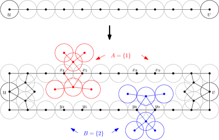
Figure 16. A path between $u$ and $v$ (top) is replaced by a corridor of the same length between $u$ and $v$ (bottom). The edges of the graph show which disks intersect or not (even if they appear to touch on the figure).

Observation 7.11.

Any $r$-corridor is a unit-disk graph, and in any unit-disk embedding of an $r$-corridor with ends $u$ and $v$, such that $u$ and $v$ lie on the outerface of the corresponding planar graph embedding, we have $d_{2}(u,v)\leq r$.

Proof.

A unit-disk embedding of an $r$-corridor is depicted in Figure 16 (bottom). The second property follows from the fact that there is a unique planar graph embedding assuming $u$ and $v$ lie on the outerface (up to homeomorphism, which follows from Theorem 2.2), and the 4 neighbors of $u$ (and $v$) are non-adjacent, and thus the minimum angle between $ux_{1}$ and $uy_{1}$ is at least $\pi$ (and similarly for the angle between $vx_{r+1}$ and $vy_{r+1}$). ∎

If an $r$-corridor with ends $u$ and $v$ is embedded as a unit-disk graph in the plane, we say that the corridor is $\delta$-tight if $r$ and $d_{2}(u,v)$ differ by at most $\delta$.

Consider a unit-disk graph $G$ embedded in the plane with a $\delta$-tight path $P^{\prime}$, for $\delta\leq 1$. Assume that $P^{\prime}$ has a subpath $P$ of length $|P|\geq|P^{\prime}|/2$, with endpoints $u,v$, such that in any unit-disk embedding of $G$, $P$ lies at Euclidean distance at least $4$ from $G-P^{\prime}$. As a subpath of $P^{\prime}$, $P$ is also $\delta$-tight. Let $G^{\prime}$ be the graph obtained from $G$ by deleting the internal vertices of $P$ and adding a copy of a $|P|$-corridor $C$ with ends $u$ and $v$. We say that we have replaced the path $P$ by the corridor $C$ in $G$.

Observation 7.12.

The graph $G^{\prime}$ is a unit-disk graph, and for any unit-disk graph embedding of $G^{\prime}$, there exist a unit-disk graph embedding of $G$ that coincides with that of $G^{\prime}$ on the vertex-set $\{u,v\}\cup(V(G)\setminus V(P))=\{u,v\}\cup(V(G^{\prime})\setminus V(C))$.

Proof.

Let $\hat{P}$ denote the polygonal chain corresponding to the embedding of $P$. Let $R$ be the region of all points at Euclidean distance at most 2 from $\hat{P}$, and at distance more than 1 from the neighbors of $u$ and $v$ not in $P$. Since $P$ lies at Euclidean distance at least $4$ from $G-P^{\prime}$, $R$ is at distance more than 1 from all points of $V(G)\setminus V(P)$. We now embed $C$ inside $R$.

Conversely, given a unit-disk embedding of $G^{\prime}$, we can simply remove $V(C)\setminus\{u,v\}$ and as by Observation 7.11, $d_{2}(u,v)\leq|P|$, we can add a path of length $|P|$ between $u$ and $v$ in the region delimited by the walls of $C$ (so the newly added vertices do not interfere with the rest of the graph). ∎

We now consider a tied-arch bridge $G$ of density $O(k^{1+\varepsilon})$, as constructed in the previous section. Recall that $G$ contains $\log k$ disjoint paths $P_{1}^{\prime},P_{2}^{\prime},\ldots$ of length $k/\log k$ with the following properties: In any unit-disk graph embedding of $G$,

• at least one of the paths $P_{i}^{\prime}$ is $O(k^{-1}\log k)$-tight and thus $O(1)$-regular, and

• Each $P_{i}^{\prime}$ contains a subpath $P_{i}$ of length at least $\tfrac{k}{2\log k}$, such that all vertices of $P_{i}$ lie at distance at least $\Omega(\tfrac{k}{\log k})$ from $G-P_{i}^{\prime}$. Moreover, if $P_{i}^{\prime}$ is $O(k^{-1}\log k)$-tight, then $P_{i}$ is also $O(k^{-1}\log k)$-tight, and in particular $O(1)$-regular.

We now replace each path $P_{i}$ in $G$ by a $|P_{i}|$-corridor $C_{i}$ as defined above. Let $G^{\prime}$ be the resulting graph (and note that $G^{\prime}$ still has $O(k^{1+\epsilon})$ vertices).

Observation 7.13.

The graph $G^{\prime}$ is a unit-disk graph, and in any unit-disk graph embedding of $G^{\prime}$, some $\Theta\left(\tfrac{k}{\log k}\right)$-corridor $C_{i}$ is $O(k^{-1}\log k)$-tight, and in particular the two walls of $C_{i}$ are $O(k^{-1}\log k)$-tight and thus $O(1)$-regular.

Proof.

By Observation 7.12 (applied to each corridor $C_{i}$), any unit-disk embedding of $G^{\prime}$ can be transformed in a unit-disk embedding of $G$ by replacing each corridor $C_{i}$ by the original path $P_{i}$ and leaving the rest of the embedding unchanged. In the resulting embedding of $G$, one of the paths $P_{i}$ is $O(k^{-1}\log k)$-tight. It follows that in the original embedding of $G^{\prime}$, the corridor $C_{i}$ is also $O(k^{-1}\log k)$-tight, and thus so are its two walls. This implies that the two walls of $C_{i}$ are $O(1)$-regular. ∎

7.7. Decorating the corridors

Now that we have found a corridor in which the walls are $O(1)$-regular, we are ready to add the gadgets that will express the disjointness. Given $A,B\subseteq\{1,\ldots,\ell\}$, one wall will belong to $L(A)$ (let us call it Alice’s wall) and the other to $R(B)$ (let us call it Bob’s wall). Intuitively, the goal of Alice (resp. Bob) will be to decorate her (his) own wall with sculptures, the locations of which are given by her subset $A$ (resp. his subset $B$). The main idea will be to make sure that a sculpture on Alice’s wall cannot be placed next to a sculpture on Bob’s wall because the corridor is too narrow for that (this corresponds to the fact that $A$ and $B$ must not intersect). One important point is that we do not know in advance which of the $O(\log k)$ corridors will have $O(1)$-regular walls, so we have to decorate all of them in advance (in the same way).

Consider an $r$-corridor $C$ in some unit-disk graph $G$, and sets $A,B\subseteq\{1,\ldots,\ell\}$, with $r\geq 4\ell+8$. Let $P_{A}=x_{1},\ldots,x_{r}$ and $P_{B}=y_{1},\ldots,y_{r}$ be the two walls of $C$. By decorating the walls of $C$ with $A$ and $B$, we mean the following: for each $1\leq i\leq\ell$,

• if $i\in A$, we add two 3-vertex paths to $G$, whose central vertices are adjacent to $x_{4i}$ and $x_{4i+1}$, (the union of the two 3-vertex paths is called a sculpture on $P_{A}$ at the $i$-th location) and

• if $i\in B$, we add two 3-vertex paths to $G$, whose central vertices are adjacent to $y_{4i}$ and $y_{4i+1}$ (the union of the two 3-vertex paths is called a sculpture on $P_{B}$ at the $i$-th location).

This is depicted in Figure 16 (bottom), with $\ell=2$, $A=\{1\}$ and $B=\{2\}$, with the sculpture on $P_{A}$ represented in red and the sculpture on $P_{B}$ represented in blue.

Observation 7.14.

If $G$ is a unit-disk graph embedded in the plane, with an $r$-corridor $C$ which is at Euclidean distance at least 3 from the vertices at distance at least 3 from $C$ in $G$, and two disjoint sets $A,B\subseteq\{1,\ldots,\ell\}$ with $r\geq 4\ell+8$, then the graph obtained from $G$ by decorating the walls of $C$ with $A$ and $B$ is a unit-disk graph.

Proof.

This follows from the definition of a corridor: the purpose of the vertices $z_{1}$ and $z_{r+1}$ is to make sure that the line segments $[x_{1},x_{r+1}]$ and $[y_{1},y_{r+1}]$ are at Euclidean distance at least $\sqrt{3}$ from each other, which allows one of the two 3-vertex paths to be placed inside the corridor while the other is placed outside, for each location $i$, as illustrated in Figure 16 (bottom). ∎

It remains to prove that when $A$ and $B$ are not disjoint, if the corridor is sufficiently tight (and the walls sufficiently regular, as a consequence), then the graph obtained by decorating the walls with $A$ and $B$ is not a unit-disk graph anymore. For this we will need to assume that $\ell$ is sufficiently small compared to the size of the corridor (but still linear in this size).

Lemma 7.15.

Let $G^{\prime}$ be the unit-disk graph with $O(k^{1+\epsilon})$ vertices from Observation 7.13. Then there is $\ell=\Omega(k/\log k)$ such that for any sets $A,B\subseteq\{1,\ldots,\ell\}$, the graph obtained from $G^{\prime}$ by decorating the walls of each of the $\Theta\left(\tfrac{k}{\log k}\right)$-corridors of $G^{\prime}$ with $A$ and $B$ is a unit-disk graph if and only if $A$ and $B$ are disjoint.

Proof.

By Observation 7.14, we only need to prove the only if direction. Fix any unit-disk embedding of the graph $G^{\prime\prime}$ obtained by decorating the walls of each of the $\log k$ many $r$-corridors of $G^{\prime}$ with $A$ and $B$, where $r=\Theta\left(\tfrac{k}{\log k}\right)$. By Observation 7.13 applied to the restriction of the unit-disk embedding to $G^{\prime}$, some $r$-corridor $C_{i}$ is $O(k^{-1}\log k)$-tight, and in particular the two walls of $C_{i}$ are $O(k^{-1}\log k)$-tight and thus $O(1)$-regular. Let $P_{A}=x_{1},\ldots,x_{r+1}$ and $P_{B}=y_{1},\ldots,y_{r+1}$ be the walls of $C_{i}$. By Lemma 7.9 there exists a constant $\alpha>0$ such that $P_{A}$ and $P_{B}$ are $\left(1/10,\alpha\tfrac{k}{\log k}\right)$-regular, so the first $\Theta(k/\log k)$ points of each of $P_{A}$ and $P_{B}$ are at Euclidean distance at most $1/10$ from their ideal points on the two line segments connecting the endpoints of $P_{A}$ and the endpoints of $P_{B}$. As these two line segments lie at distance at most 2 apart, this does not leave enough space to place a sculpture on $P_{A}$ and a sculpture on $P_{B}$ at the same location $i$, as two vertices from these sculptures would be at distance at most 1 from each other (while these vertices are non adjacent in the graph). ∎

The graph $G^{\prime}$ from Lemma 7.15 is illustrated in Figure 10.

7.8. Disjointness-expressivity of unit-disk graphs

We are now ready to prove the main result of this section.

Theorem 7.16.

For any $\delta>0$, the class of unit-disk graphs is $(O(\log n),1-\delta)$-disjointness-expressing.

Proof.

Let $N$ be a natural integer and $A,B\subseteq\{1,\ldots,N\}$. Let $k$ be such that $N=\Theta\left(\tfrac{k}{\log k}\right)$ and such that we can apply Lemma 7.15 with $\ell=N$, which gives us a graph $G^{\prime}_{A,B}$ where each of the corridors is decorated with $A$ and $B$. Observe that $G^{\prime}_{A,B}$ contains $\log k$ corridors, each of length $\Theta\left(\tfrac{k}{\log k}\right)$. Before decoration, the graph has $O(k^{1+\epsilon})$ vertices so, even after decorating the walls of the corridors, the resulting graph $G^{\prime}_{A,B}$ still contains $O\left(k^{1+\epsilon}\right)$ vertices. It follows that the graphs have at most $O((N\log N)^{1+\epsilon})=O(N^{1+\delta})$ vertices for any $\delta>\epsilon$.

For a corridor $C$ in $G^{\prime}_{A,B}$, let $P_{A}$ be the wall of $C$ decorated with $A$, and let $P_{A}^{-}$ be $P_{A}$ minus its two endpoints (i.e., if $P_{A}$ consists of the path $x_{1},\ldots,x_{r+1}$ plus decorations, then $P_{A}^{-}=P_{A}-\{x_{1},x_{r+1}\}$). We say that $P_{A}^{-}$ is a reduced decorated wall, with endpoints $x_{2}$ and $x_{r}$. We define $L(A)$ to be the subgraph of $G^{\prime}_{A,B}$ induced by the union of the reduced decorated walls $P_{A}^{-}$ in each of the corridors of $G^{\prime}_{A,B}$. We then define the set of special vertices $S$ as the union of all endpoints of the reduced decorated walls $P_{A}^{-}$. The graph $R(B)$ is then defined as the subgraph of $G^{\prime}_{A,B}$ induced by $V(G^{\prime}_{A,B})\setminus L(A))\cup S$.

By construction, $G^{\prime}_{A,B}$ is the graph $g(L(A),R(B))$ obtained from $L(A)$ and $R(B)$ by gluing them along $C$. As there are $\log k=O(\log N)$ corridors and the closed neighborhood of each vertex of $S$ contains 4 vertices, the size of $N[S]$ is $O(\log N)$. The fact that $G^{\prime}_{A,B}$ is a unit-disk graph if and only if $A$ and $B$ are disjoint is a direct consequence of Lemma 7.15. ∎

Using Theorem 4.2, together with Corollary 3.3, we immediately deduce the following.

Theorem 7.17.

The local complexity of the class of unit-disk graphs is $O(n\log n)$ and $\Omega(n^{1-\delta})$ for any $\delta>0$.

8. Open problems

In this paper we have obtained a number of optimal (or close to optimal) results on the local complexity of geometric graph classes. Our proofs are based on a new notion of rigidity. It is natural to ask which other graph classes enjoy similar properties. A natural candidate is the class of segment graphs (intersection graphs of line segments in the plane), which have several properties in common with unit-disk graphs, in particular the recognition problems for these classes are $\exists\mathbb{R}$-complete (i.e., complete for the existential theory of the reals) and the minimum bit size for representing an embedding of some of these graphs in the plane is at least exponential in $n$. We believe that the local complexity of segment graphs (and that of the more general class of string graphs) is at least polynomial in $n$. More generally, is it true that all classes of graphs for which the recognition problem is hard for the existential theory of the reals have polynomial local complexity?

It might also be interesting to investigate the smaller class of circle graphs (intersection graphs of chords of a circle). The authors of [14] proved that the closely related class of permutation graphs has logarithmic local complexity. It is quite possible that the same holds for circle graphs. See [15] for results on interactive proof labeling schemes for this class and related classes.

We proved that 1-planar graphs have local complexity $\Theta(n)$. What can we say about the local complexity of other graph classes defined with constrained on their drawings in the plane? For instance is it true that for every $k\geq 2$, the local complexity of the class of graphs with queue number at most $k$ is polynomial? What about graphs with stack number at most $k$?

We have given the first example of non-trivial hereditary (and even monotone) classes of local complexity $\Omega(n)$. Can this be improved? Are there hereditary (or even monotone) classes of local complexity $\Omega(n^{c})$ for $c>1$?

Appendix A Proofs from Section 7.3

See 7.2

Proof.

Consider a $(k,\delta)$-almost-equilateral embedding of a stripe $S_{\ell}$ with $k\gg\delta$. Up to exchanging the roles of $u_{i}$ and $v_{i}$, the Euclidean distance between $u_{0}$ and $u_{\ell}$ is minimized when the distances $d_{2}(u_{i},u_{i+1})$ ($0\leq i\leq\ell-1$) are minimized and the angles $\angle u_{i-1}u_{i}u_{i+1}$ ($1\leq i\leq\ell-1$) are maximized. Since all the constraints on these distances and angles are local, in an embedding minimizing $d_{2}(u_{0},v_{\ell})$ all these lengths are equal, and all these angles are equal. It follows that the Menger curvature of all consecutive triples is the same (and only depends on $k$ and $\delta$, since the local constraints only depend on $k$ and $\delta$). ∎

See 7.3

Proof.

Consider a $(k,\delta)$-almost-equilateral embedding of $S_{\ell}$ where $d_{2}(u_{0},v_{\ell})\leq m+1$. The second part of the statement simply follows from the fact that in any $(k,\delta)$-almost-equilateral embedding of $S_{\ell}$, the diameter of the corresponding point set is at most $(k+\delta)\ell$, so we only need to prove the first part of the statement. We only give the main steps of the proof and omit the technical computations. By Lemma 7.3, for each $0\leq i<j\leq\ell$, the Euclidean distance between $u_{i}$ and $u_{j}$ is at least the distance between the endpoints of some circular arc of radius $\rho$ that subtends an angle $\tfrac{j-i}{\ell}\cdot\pi$, that is $d_{2}(u_{i},u_{j})\geq 2\rho\sin(\tfrac{j-i}{\ell}\cdot\tfrac{\pi}{2})$. It follows that for any $0\leq i\leq\ell$, $d_{2}(u_{0},u_{i})\geq 2\rho\sin(\alpha)$ and $d_{2}(u_{0},u_{i})\geq 2\rho\cos(\alpha)$, where $\alpha:=\tfrac{i\pi}{2\ell}$. We can use this to estimate the area of the triangle $u_{0}u_{i}u_{\ell}$

1. when $u_{0},u_{i},u_{\ell}$ all lie on a circle of radius $\rho$ and $d_{2}(u_{0},u_{\ell})=2\rho$, and

2. when we only require that $d_{2}(u_{0},u_{\ell})=2\rho+O(k)$.

Comparing the two areas (more precisely, in the second case, we only obtain a lower bound on the area), we can estimate the distance between $u_{i}$ and the segment $[u_{0}u_{\ell}]$ in both cases and then show that these distances differ by at most $O(k)$. We use this to conclude that in the second case, $u_{i}$ lies at distance $O(k)$ from the circle of radius $\rho$ centered in $c$. ∎

Appendix B Proofs from Section 7.4

See 7.4

Proof.

Consider a unit-disk graph embedding of $T_{n}$, and let $P$ be the $(8n+16)$-gon corresponding to the vertices of $C$. We denote by $P_{1}$ and $P_{2}$ the two polygonal subchains of $P$ with endpoints $c$ and $c^{\prime}$. Let $R_{1}$ be the region bounded by $P_{1}$ and the line-segment $[c,c^{\prime}]$, and let $R_{2}$ be the region bounded by $P_{2}$ and the line-segment $[c,c^{\prime}]$. It might be the case that one of the two regions contains the other, but in any case the region $R$ bounded by $P$ is contained in the union of $R_{1}$ and $R_{2}$.

Note that $T_{n}$ has an independent set $S$ of size at least $(2n+2)^{2}$ (the set of red vertices, or the set of blue vertices in Figure 12). Discard the vertices of $S$ that are at Euclidean distance at most $\tfrac{1}{2}$ from $P$ or from the line-segment $[c,c^{\prime}]$ (there are at most $O(n)$ such vertices), and let $S^{\prime}$ be the resulting independent set (of size $(2n+2)^{2}-O(n)$). The disks of radius $\tfrac{1}{2}$ centered in the points corresponding to $S^{\prime}$ are pairwise disjoint, and all contained in $R$, and thus contained in $R_{1}$ or $R_{2}$. It follows that one of $R_{1}$ or $R_{2}$ (say $R_{1}$), contains at least $\tfrac{1}{2}(2n+2)^{2}-O(n)=2(n+1)^{2}-O(n)$ disjoint disks of radius $\tfrac{1}{2}$, and thus has area $A(R_{1})\geq\tfrac{\pi}{4}(2(n+1)^{2}-O(n))=\tfrac{\pi}{2}(n+1)^{2}-O(n)$. Let $d:=d_{2}(c,c^{\prime})$. Note that $R_{1}$ and $R_{2}$ have perimeter at most $4n+8+d$, and thus by the isoperimetric inequality in the plane, $A(R_{1})\leq\tfrac{1}{4\pi}(4n+8+d)^{2}$. It follows that $(4n+d+8)^{2}\geq 2\pi^{2}(n+1)^{2}-O(n)$, and thus $d\geq(\pi\sqrt{2}-4)n-O(\sqrt{n})=\Omega(n)$, as desired. ∎

Appendix C Proofs from Section 7.5

See 7.6

Proof.

Let $y$ be the length of the altitude of $abc$ passing through $c$. Note that $y$ is maximized when $d_{2}(a,c)=d_{2}(b,c)$, and thus by Pythagora’s theorem, $y\leq\sqrt{\delta x/2}+O(x^{-1/2})$. Note that subject to the conditions above, $\min\{d_{2}(a,c)-d_{2}(a,c^{\prime}),d_{2}(b,c)-d_{2}(b,c^{\prime})\}$ is maximized when $d_{2}(c,c^{\prime})=\rho$. Let $c^{*}$ be the point of the altitude of $abc$ passing through $c$ such that $d_{2}(c,c^{*})=\rho$. This altitude divides $abc$ into two triangles, say $T_{a}$ containing $a$ and $T_{b}$ containing $b$. If $c^{\prime}\in T_{a}$ then $d_{2}(b,c^{\prime})\geq d_{2}(b,c^{*})$, and if $c^{\prime}\in T_{b}$ then $d_{2}(a,c^{\prime})\geq d_{2}(a,c^{*})$. Thus it suffices to prove that $d_{2}(a,c)-d_{2}(a,c^{*})\leq\rho\sqrt{2\delta/x}+O(1/x)$ and $d_{2}(b,c)-d_{2}(b,c^{*})\leq\rho\sqrt{2\delta/x}+O(1/x)$. The two cases being symmetric, we only prove the former. Let $z=d_{2}(a,c)$. By Pythagora’s theorem,

$$d_{2}(a,c^{*})^{2}=z^{2}-2\rho y+\rho^{2}=z^{2}\left(1-\frac{2\rho y}{z^{2}}+\frac{\rho^{2}}{z^{2}}\right).$$

As $z=\Omega(x)$, it follows that

$$d_{2}(a,c^{*})=z\sqrt{1-\frac{2\rho y}{z^{2}}+\frac{\rho^{2}}{z^{2}}}=z\left(1-\frac{\rho y}{z^{2}}+O(x^{-2})\right)=z-\rho\sqrt{2\delta/x}+O(x^{-1}).$$

So, $d_{2}(a,c)-d_{2}(a,c^{*})\leq\rho\sqrt{2\delta/x}+O(1/x)=O(\sqrt{\delta/x})$, as desired. ∎

See 7.7

Proof.

Let $x:=d_{2}(a,b)$, and let $c\in\mathbb{R}^{2}$ be such that $d_{2}(a,c)=|P_{\mathbf{x}0}|$ and $d_{2}(b,c)=|P_{\mathbf{x}1}|$. There are two choices for $c$ which are symmetric with respect to the line-segment $[a,b]$, and we take the one which is closest from $z$. The path $P_{\mathbf{x}}$ is $\delta$-tight so $d_{2}(a,c)+d_{2}(c,b)=x+\delta$. As $c^{\prime}$ is a midpoint of $P_{\mathbf{x}}$, $|d_{2}(a,c)-d_{2}(b,c)|\leq 1$. Hence, in order to apply Lemma 7.6, which directly gives us the desired result, we only need to prove that $\rho:=d_{2}(c,c^{\prime})=O(1)$.

Let $m_{i}^{*}$ denote the minimum distance between $z$ and $c^{\prime}$ in a unit-disk embedding of $G_{i}$ and observe that we have $m_{i}^{*}\leq d_{2}(z,c)\leq d_{2}(z,c^{\prime})$. By definition, the path in $G_{i+1}$ linking $z$ and $c^{\prime}$ has length $\lceil m_{i}^{*}\rceil$ so as $G_{i+1}$ is a unit-disk graph, $d_{2}(z,c^{\prime})\leq\lceil m_{i}^{*}\rceil$. Thus $d_{2}(z,c)\leq d_{2}(z,c^{\prime})\leq\lceil d_{2}(z,c)\rceil$.

Let $R_{a}$ be the disk of radius $d_{2}(a,c)$ centered in $a$ and let $R_{b}$ be the disk of radius $d_{2}(b,c)$ centered in $b$. Let $R_{z}$ be the disk of radius $\lceil d_{2}(z,c)\rceil\leq d_{2}(z,c)+1$ centered in $z$. Note that since $G_{0}$ is a unit-disk graph, $c^{\prime}$ lies in $R_{a}\cap R_{b}\cap R_{z}$. Recall that $z$ lies at distance $\Omega(k)=\Omega(x)$ from $c$ and at distance at most $\tfrac{1}{2}$ from the perpendicular bisector of the line-segment $[a,b]$. It then follows from Pythagora’s theorem that $\rho=d_{2}(c,c^{\prime})\leq 1+O(x^{-1})=O(1)$, as desired. ∎

See 7.8

Proof.

For the base case of the induction, we start by recalling that in any unit-disk embedding of $G_{0}$, $P$ is 1-tight. Assume now that $i\geq 1$ and the result holds in $G_{i-1}$. Fix a unit-disk embedding of $G_{i}$ and consider the restriction of this unit-disk embedding to $G_{i-1}$. By the induction hypothesis there is $\mathbf{x}\in\{0,1\}^{i-1}$ such that $|P_{\mathbf{x}}|\leq d_{2}(a,b)+\delta$ with $\delta\leq\alpha\cdot 2^{i-1}\cdot k^{2^{-i+1}-1}$, for some constant $\alpha>0$, where $a$ and $b$ denote the endpoints of $P_{\mathbf{x}}$. Let $c^{\prime}$ be the midpoint of $P_{\mathbf{x}}$ used to split it into $P_{\mathbf{x}0}$ and $P_{\mathbf{x}1}$ in $G_{i}$. As $d_{2}(a,b)\geq k2^{-i}$, we have

$$\sqrt{\delta/d_{2}(a,b)}\leq\frac{\alpha^{1/2}\cdot 2^{i/2}\cdot k^{2^{-i}-1/2}}{k^{1/2}2^{-i/2}}\leq\alpha^{1/2}\cdot 2^{i}\cdot k^{2^{-i}-1},$$

By Corollary 7.7, we have that $|P_{\mathbf{x}0}|\leq d_{2}(a,c^{\prime})+O(\sqrt{\delta/d_{2}(a,b)})$, or $|P_{\mathbf{x}1}|\leq d_{2}(b,c^{\prime})+O(\sqrt{\delta/d_{2}(a,b)})$. By taking $\alpha$ sufficiently large compared to the implicit constant in the $O(\sqrt{\delta/d_{2}(a,b)})$ term from Corollary 7.7, we obtain that $|P_{\mathbf{x}0}|\leq d_{2}(a,c^{\prime})+\alpha\cdot 2^{i}\cdot k^{2^{-i}-1}$, or $|P_{\mathbf{x}1}|\leq d_{2}(b,c^{\prime})+\alpha\cdot 2^{i}\cdot k^{2^{-i}-1}$ as desired. ∎

See 7.9

Proof.

Note that $\ell-\delta\leq d_{2}(v_{1},v_{\ell+1})\leq\ell$. We place $\ell+1$ evenly spaced points $u_{1},\ldots,u_{\ell+1}$ on the line-segment $[v_{1},v_{\ell+1}]$ with $u_{1}=v_{1}$, $u_{\ell+1}=v_{\ell+1}$. For $2\leq i\leq\ell+1$, the distance $d_{2}(u_{i},v_{i})$ is maximized when $i=\left\lceil\frac{\ell+1}{2}\right\rceil$, and is at most the distance between the middle of the line-segment $[v_{1},v_{\ell+1}]$ and a point $c$ at Euclidean distance $\ell/2$ from $v_{1}$ and $v_{\ell+1}$. By Pythagora’s theorem, this distance is at most $\gamma:=\sqrt{\ell^{2}/4-(\ell-\delta)^{2}/4}=\sqrt{\ell\delta/2}+O(\ell^{-1/2})$, as desired.

For the second part of the lemma, we observe that each vertex $v_{i}$ satisfies $d_{2}(v_{i},v_{1})+d_{2}(v_{i},v_{\ell+1})\leq\ell$, so each such point is contained in the region bounded by the ellipse with foci $v_{1}$ and $v_{\ell+1}$, width $\ell$, and height at most $2\gamma$ (by the preceding paragraph). Let $m$ denote the midpoint of the line segment $[v_{1},v_{\ell+1}]$. Let $p$ be a point on the ellipse, and let $p^{\prime}$ be the projection of $p$ on the line $(v_{1},v_{\ell+1})$. By the standard description of an ellipse in Cartesian coordinates, if $x:=d_{2}(m,p^{\prime})$ then $y:=d_{2}(p,p^{\prime})=\tfrac{2\gamma}{\ell}\sqrt{\ell^{2}/4-x^{2}}$. If we take $(1-\alpha)\ell/2\leq x\leq\ell/2$ for some $\alpha>0$, then $y\leq\gamma\sqrt{1-(1-\alpha)^{2}}=\lambda^{\prime}\gamma$ for $\lambda^{\prime}:=\sqrt{2\alpha-\alpha^{2}}$ independent of $\ell$ and $\delta$. Let $p^{\prime\prime}$ be the point of $[v_{1},v_{\ell+1}]$ at distance $\tfrac{\ell-\delta}{\ell}d_{2}(v_{1},p)$ from $v_{1}$. Then $d_{2}(p^{\prime},p^{\prime\prime})\leq d_{2}(v_{1},p)-\tfrac{\ell-\delta}{\ell}d_{2}(v_{1},p)=\tfrac{\delta}{\ell}d_{2}(v_{1},p)$. It then follows from Pythagora’s theorem that $d_{2}(p,p^{\prime\prime})\leq\sqrt{\lambda^{\prime 2}\gamma^{2}+\tfrac{\delta^{2}}{\ell^{2}}d_{2}(v_{1},p)^{2}}$. If $d_{2}(v_{1},p)\leq\alpha\ell$ then $d_{2}(p,p^{\prime\prime})\leq\sqrt{\lambda^{\prime 2}\gamma^{2}+\alpha^{2}\delta^{2}}\leq\sqrt{\lambda^{\prime 2}\gamma^{2}+\alpha^{2}}$ since $\delta\leq 1$. By considering $p$ above as the location of $v_{i}$ ($1\leq i\leq\alpha\ell$) that maximizes its distance to $u_{i}$ (whose location corresponds to $p^{\prime\prime}$ above), we conclude that $d_{2}(v_{i},u_{i})\leq\sqrt{\lambda^{\prime 2}\gamma^{2}+\alpha^{2}}=\sqrt{(2\alpha-\alpha^{2})\gamma^{2}+\alpha^{2}}$, as desired. ∎

References

- [1] Noga Alon and Andrey Kupavskii. Two notions of unit distance graphs. Journal of Combinatorial Theory, Series A, 125:1–17, 2014.
- [2] Édouard Bonnet, Colin Geniet, Eun Jung Kim, Stéphan Thomassé, and Rémi Watrigant. Twin-width II: small classes. Combinatorial Theory, 2(2):#10, 2022.
- [3] Nicolas Bousquet, Laurent Feuilloley, and Théo Pierron. Local certification of graph decompositions and applications to minor-free classes. In Quentin Bramas, Vincent Gramoli, and Alessia Milani, editors, 25th International Conference on Principles of Distributed Systems, OPODIS 2021, December 13-15, 2021, Strasbourg, France, volume 217 of LIPIcs, pages 22:1–22:17. Schloss Dagstuhl - Leibniz-Zentrum für Informatik, 2021.
- [4] Keren Censor-Hillel, Ami Paz, and Mor Perry. Approximate proof-labeling schemes. Theoretical Computer Science, 811:112–124, 2020.
- [5] Pierluigi Crescenzi, Pierre Fraigniaud, and Ami Paz. Trade-offs in distributed interactive proofs. In Jukka Suomela, editor, 33rd International Symposium on Distributed Computing, DISC 2019, October 14-18, 2019, Budapest, Hungary, volume 146 of LIPIcs, pages 13:1–13:17. Schloss Dagstuhl - Leibniz-Zentrum für Informatik, 2019.
- [6] Louis Esperet and Benjamin Lévêque. Local certification of graphs on surfaces. Theoretical Computer Science, 909:68–75, 2022.
- [7] Laurent Feuilloley. Introduction to local certification. Discrete Mathematics & Theoretical Computer Science, 23(3), 2021.
- [8] Laurent Feuilloley, Nicolas Bousquet, and Théo Pierron. What can be certified compactly? Compact local certification of MSO properties in tree-like graphs. In Alessia Milani and Philipp Woelfel, editors, PODC ’22: ACM Symposium on Principles of Distributed Computing, Salerno, Italy, July 25 - 29, 2022, pages 131–140. ACM, 2022.
- [9] Laurent Feuilloley, Pierre Fraigniaud, Pedro Montealegre, Ivan Rapaport, Éric Rémila, and Ioan Todinca. Compact distributed certification of planar graphs. Algorithmica, 83(7):2215–2244, 2021.
- [10] Laurent Feuilloley, Pierre Fraigniaud, Pedro Montealegre, Ivan Rapaport, Éric Rémila, and Ioan Todinca. Local certification of graphs with bounded genus. Discrete Applied Mathematics, 325:9–36, 2023.
- [11] Pierre Fraigniaud, Frédéric Mazoit, Pedro Montealegre, Ivan Rapaport, and Ioan Todinca. Distributed certification for classes of dense graphs. arXiv preprint arXiv:2307.14292, 2023.
- [12] Pierre Fraigniaud, Pedro Montealegre, Ivan Rapaport, and Ioan Todinca. A meta-theorem for distributed certification. In Merav Parter, editor, Structural Information and Communication Complexity - 29th International Colloquium, SIROCCO 2022, Paderborn, Germany, June 27-29, 2022, Proceedings, volume 13298 of Lecture Notes in Computer Science, pages 116–134. Springer, 2022.
- [13] Mika Göös and Jukka Suomela. Locally checkable proofs in distributed computing. Theory of Computing, 12(1):1–33, 2016.
- [14] Benjamin Jauregui, Pedro Montealegre, Diego Ramírez-Romero, and Ivan Rapaport. Local certification of some geometric intersection graph classes. CoRR, abs/2309.04789, 2023.
- [15] Benjamin Jauregui, Pedro Montealegre, and Ivan Rapaport. Distributed interactive proofs for the recognition of some geometric intersection graph classes. In Merav Parter, editor, Structural Information and Communication Complexity - 29th International Colloquium, SIROCCO 2022, Paderborn, Germany, June 27-29, 2022, Proceedings, volume 13298 of Lecture Notes in Computer Science, pages 212–233. Springer, 2022.
- [16] Gillat Kol, Rotem Oshman, and Raghuvansh R. Saxena. Interactive distributed proofs. In Calvin Newport and Idit Keidar, editors, Proceedings of the 2018 ACM Symposium on Principles of Distributed Computing, PODC 2018, Egham, United Kingdom, July 23-27, 2018, pages 255–264. ACM, 2018.
- [17] Amos Korman, Shay Kutten, and David Peleg. Proof labeling schemes. Distributed Computing, 22(4):215–233, 2010.
- [18] Vladimir P. Korzhik. Minimal non-1-planar graphs. Discrete Mathematics, 308(7):1319–1327, 2008.
- [19] László Lovász. Communication complexity: A survey. Forschungsinst. für Diskrete Mathematik. Inst. für Ökonometrie u. Operations, 1989.
- [20] Colin McDiarmid and Tobias Müller. The number of disk graphs. European Journal of Combinatorics, 35:413–431, 2014. Selected Papers of EuroComb’11.
- [21] Moni Naor, Merav Parter, and Eylon Yogev. The power of distributed verifiers in interactive proofs. In Shuchi Chawla, editor, Proceedings of the 2020 ACM-SIAM Symposium on Discrete Algorithms, SODA 2020, Salt Lake City, UT, USA, January 5-8, 2020, pages 1096–115. SIAM, 2020.
- [22] Jaroslav Nešetřil and Patrice Ossona De Mendez. Sparsity: graphs, structures, and algorithms, volume 28. Springer Science & Business Media, 2012.
- [23] Neil Robertson and Paul D. Seymour. Graph minors. XX. Wagner’s conjecture. Journal of Combinatorial Theory, Series B, 92(2):325–357, 2004.
- [24] Hassler Whitney. 2-isomorphic graphs. American Journal of Mathematics, 55(1):245–254, 1933.