The Sky’s the Limit: Re-lightable Outdoor Scenes via a
Sky-pixel Constrained Illumination Prior and Outside-In Visibility

Abstract

Inverse rendering of outdoor scenes from unconstrained image collections is a challenging task, particularly illumination/albedo ambiguities and occlusion of the illumination environment (shadowing) caused by geometry. However, there are many cues in an image that can aid in the disentanglement of geometry, albedo and shadows. We exploit the fact that any sky pixel provides a direct measurement of distant lighting in the corresponding direction and, via a neural illumination prior, a statistical cue as to the remaining illumination environment. We also introduce a novel ‘outside-in’ method for computing differentiable sky visibility based on a neural directional distance function. This is efficient and can be trained in parallel with the neural scene representation, allowing gradients from appearance loss to flow from shadows to influence estimation of illumination and geometry. Our method estimates high-quality albedo, geometry, illumination and sky visibility, achieving state-of-the-art results on the NeRF-OSR relighting benchmark. Our code and models can be found here.

1 Introduction

Inverse rendering of outdoor scenes has diverse downstream applications such as scene relighting, augmented reality, game asset generation, and environment capture for films and virtual production. However, accurately estimating the underlying scene model that produced an image is an inherently ambiguous task due to its ill-posed nature [2]. To address this, many works use some combination of handcrafted [7, 17] or learned priors [44, 4, 6, 20], inductive biases in model architectures [13], or multi-stage training pipelines [34, 48]. This process is made even more difficult when considering in-the-wild image collections from the internet that contain transient objects, image filters, unknown camera parameters and changes in illumination.

Outdoor scenes present particular challenges. Natural illumination from the sky is complex and exhibits enormous dynamic range. This causes strong cast shadows when the brightest parts of the sky are occluded. These occlusions are non-local and discontinuous making them hard to incorporate within a differentiable renderer. Outdoor scene geometry can also exhibit arbitrary ranges of scale. On the other hand, sky illumination dominates secondary bounce lighting, meaning it is reasonable to assume a spatially non-varying, distant illumination environment. In addition, natural illumination contains statistical regularities [14] that make it easier to model. For example, luminance generally increases with elevation (the ‘lighting-from-above’ prior), the sun can only be in one position and the range of possible colours from sun and sky light is limited.

In this paper, we tackle the outdoor scene inverse rendering problem by fitting a neural scene representation to a multi-view, varying-illumination photo collection. We name our method NeuSky, and make three key contributions relative to prior work. First, we exploit statistical and geometric (rotation equivariance) regularities in outdoor lighting by using a neural HDR illumination model [16] learnt from natural environments. Second, we make a key observation. Any pixel in an image that observes the sky provides a direct constraint on the illumination environment in that direction. Foreground scene pixels additionally indirectly constrain the illumination environment via their shading. Together these constraints allow us to estimate realistic illumination environments and reduce lighting/albedo ambiguities. Finally, we propose a novel differentiable, neural approximation to sky visibility, computed with a single forward pass through a directional distance function network. This allows us to render scene points with the estimated neural environment lighting, accounting for occlusions by other parts of the scene. Our neural scene representation and neural visibility model can be trained end-to-end, simultaneously without the need for phased training. Crucially, this means that shadows can influence illumination and geometry estimation by appearance losses backpropagating through the visibility network, also avoiding shadow baking into albedo.

Figure 2: We surround our NeuS-Facto [45] volume with two spherical neural fields at radius $1$ and radius $\infty$ modelling sky visibility and distant illumination respectively. Blue arrows correspond to rays sampling distant illumination. Pink circles and Maroon arrows are position and direction samples of our sky visibility network. In a given direction, visibility changes with position but distant illumination does not. For speed we only sample sky visibility on the surface of our scene, Green circles, and distribute this visibility to all samples, Orange circles, along a ray.

2 Related Work

Relightable Neural Scenes    The core NeRF [25] approach has been improved in several key ways since its publication. Nerfstudio, [35] a platform for researching in Neural Fields, introduced NeRFacto taking advantage of many of these developments. It leverages the same proposal sampling and scene contraction as Mip-NeRF 360 [3] alongside the hash-grid representation from Instant-NGP [26] to reduce network sizes and vastly speed up training. Implicit surface representations were introduced in NeuS [37], which used a neural Signed Distance Function (SDF) with NeRF volume rendering. NeuS-Facto, introduced in SDFStudio [45], combined the NeRFacto improvements with NeuS and is the underlying model that we use.

In parallel with these developments, several attempts have been made to use neural scene representations for decomposition into its intrinsic properties. NeRF-OSR [29] predicts albedo and density. For distant illumination, they predict per image Spherical Harmonic (SH) lighting coefficients and model illumination-dependent shadows via a shadow network conditioned on those SH coefficients. Whilst now providing a parametric model of illumination they are limited by the quality of normals obtained from NeRF density (we use a NeuS derivative with high-quality geometry), shadows that are not related to the scene geometry (our shadow network is directly tied to scene geometry) and the low frequency of SH (we employ a neural field for illumination capable of capturing higher order lighting effects). Methods such as PhySG [47] and NeRF-V [34] allow relighting but require known illumination. NeRFactor [48] additionally optimises visibility and illumination together allowing shadows but with a low-resolution environment map and no illumination prior. Similar to our work, FEGR [39] also uses a neural field representation for HDR illumination, however, they do not include a prior over illuminations. Their rasterisation process to model visibility is also a non-differentiable function, meaning cues from shading and shadows will not inform illumination or geometry estimations. Also similar to our work, NeuLighting [21] uses prior over illuminations and visibility MLP but their framework is trained in a cascaded manner, similar to NeRF-V, so visibility can not influence lighting and geometry estimations compared to our method, furthermore their method considers shadows only from the sun.

Directional Distance Fields    SDFs measure the distance to the nearest surface at a given point, signed to indicate outside/inside. In contrast, Directional Distance Functions (DDFs) measure the distance to the nearest surface in a given direction, making them 5D as opposed to 3D functions for SDFs. Interest in DDFs has primarily been as a geometry representation that allows faster rendering (no sphere tracing is required). Neural DDFs were primarily introduced in [50] which developed the Signed Directional Distance Functions as a model of continuous distance view synthesis and derived many important properties of SDDFs. This was later extended by [1], which enabled the modelling of internal structures via dropping the sign and extending the representation via probabilistic modelling. Subsequent works enable to model of shapes with no explicit boundary surface [36], refine the multi-view consistency of DDFs [22] and employ SDDFs to improve optimisation of multi-view shape reconstruction [49]. Our usage of a DDF is most similar to that of FiRE [43] which also combines an SDF scene representation with a DDF sampled only on the unit sphere. However, unlike FiRE, whose goal was fast rendering, we show how to use a spherical DDF for fast, differentiable sky visibility. A more in-depth explanation of DDFs is found in Section 3.2.

Neural Illumination and Visibility    Boss et al. [5] proposed neural pre-integrated lighting (PIL), a spherical neural field conditioned on a roughness parameter to model an illumination environment convolved with a BRDF. This enabled fast rendering but at the expense of being unable to model occlusions of the illumination environment. RENI  [15], proposed by Gardner et al., is a vertical-axis rotation-equivariant conditional spherical neural field, trained on thousands of HDR outdoor environment maps to learn a prior for natural illumination. The low-dimensional but expressive latent space is useful for constraining inverse rendering problems. This was subsequently extended in RENI++ [16] with the addition of scale-invariant training and a transformer-based architecture. Several other recent methods aim to predict illumination from small image crops [33, 12], as a 5D light field network [42], from a text description [10] or using diffusion models with differentiable path tracing [18]. Rhodin et al. [28] approximate scene geometry with Gaussian blobs for differentiable visibility. Lyu et al. [24] similarly use spheres for geometry and model illumination with spherical harmonics for approximate differentiable shadows. Worchel and Alexa [41] use a differentiable mesh renderer for classical shadow mapping [40].

3 Method

Our method takes as input a dataset of $N$ images. From these images we compute poses with COLMAP [30, 31] and semantic segmentation maps with ViT-Adapter [9] according to the Cityscapes [11] convention. The preprocessed dataset comprises $\mathcal{D}=\left\{(\mathcal{I}_{i},\mathbf{E}_{i},\mathbf{K}_{i},\mathcal{S}_{i})\right\}_{i=1}^{N}$, where $\mathcal{I}\in{\mathbb{R}}^{H\times W\times 3}$ is an image, $\mathcal{S}\in\mathbb{Z}^{H\times W}$ is the segmentation map and $\mathbf{E}=\left[\mathbf{R}|\mathbf{t}\right]\in{\mathbb{R}}^{3\times 4}$ and $\mathbf{K}\in{\mathbb{R}}^{3\times 3}$ are the camera extrinsics and intrinsics respectively. To align the vertical axis of our scene with gravity, we robustly fit a plane to the camera positions and rotate to align with the $x$-$y$ plane.

Scene Representation    We model scene geometry as a neural SDF, such that at any point $\mathbf{x}\in{\mathbb{R}}^{3}$, the signed distance is given by $f_{\text{SDF}}(\mathbf{x})\in{\mathbb{R}}$. We assume that the scene is Lambertian, with diffuse albedo modelled by the neural field $\mathbf{a}(\mathbf{x})\in[0,1]^{3}$. We also assume that illumination is a distant environment that depends only on direction $\mathbf{d}\in S^{2}$, with HDR RGB incident radiance given by $L_{i}(\mathbf{d})\in{\mathbb{R}}_{\geq 0}^{3}$.

Rendering    We follow NeuS [38] and derive a volume density, $\sigma(\mathbf{x})$, from the SDF value. This allows volume rendering of the SDF in the same fashion as in NeRF. For a ray $\mathbf{r}$ with origin $\mathbf{o}$ and direction $\mathbf{v}$, the time-discrete volume rendered RGB colour is given by:

$$\mathbf{c}(\mathbf{r})\!=\!\!\sum_{j=1}^{S}\!w_{j}\mathbf{a}(\mathbf{x}_{j})\!\sum_{k=1}^{D}\!L_{i}(\mathbf{d}_{k})V(\mathbf{x}_{E},\mathbf{d}_{k})\!\max(0,\mathbf{n}(\mathbf{x}_{j})\cdot\mathbf{d}_{k}),$$ (1)

where the first summation is over the $S$ samples along the ray, while the second is over the $D$ lighting direction samples. The lighting direction samples are distributed approximately uniformly over the sphere by using an $8$-subdivided icosahedron giving $D=642$. $w_{j}$ is the volume rendering blending weight for the $j$th sample point which depends on $t_{1\dots j}$ and $\sigma(\mathbf{x}_{1\dots j})$, with $\mathbf{x}_{j}=\mathbf{o}+t_{j}\mathbf{v}$. $V(\mathbf{x},\mathbf{d})\in\{0,1\}$ is the sky visibility in direction $\mathbf{d}$ at position $\mathbf{x}$ and $\mathbf{n}(\mathbf{x})=\nabla f_{\text{SDF}}(\textbf{x})/\|\nabla f_{\text{SDF}}(\textbf{x})\|$ is the surface normal at $\mathbf{x}$, derived from the gradient of the SDF.

We define our appearance loss for a batch of rays $\mathcal{R}$ as:

$$\mathcal{L}_{\text{app}}=\sum_{\mathbf{r}\in\mathcal{R}}\varepsilon(\mathbf{c}_{\text{gt}}(\mathbf{r}),\text{sRGB}(\mathbf{c}(\mathbf{r}))),$$ (2)

where $\mathbf{c}_{\text{gt}}(\mathbf{r})$ is the ground truth colour for ray $\mathbf{r}$, $\text{sRGB}(\cdot)$ tonemaps the linear image provided by our model and $\varepsilon$ computes the sum of L1 and cosine errors (to match both absolute RGB values and hue). To avoid overfitting we apply a random rotation $R\sim\mathcal{U}(SO(3))$ to jitter the direction vectors $\mathbf{d}_{k}$ in every batch.

Neural Illumination Model    To restrict $L_{i}$ to the space of plausible natural illumination environments, we use a neural illumination prior, RENI++ [16]. This is a conditional neural field, $f_{L_{i}}:S^{2}\times{\mathbb{R}}^{3\times K}\rightarrow{\mathbb{R}}^{3}$ that outputs log HDR RGB colours in the given input direction, conditioned on a normally distributed 3D latent code $\mathbf{Z}\in{\mathbb{R}}^{3\times K},\text{vec}(\mathbf{Z})\sim\mathcal{N}(\mathbf{0}_{3K},\mathbf{I}_{3K})$. The latent space of RENI++ provides a low dimensional characterisation of natural, outdoor illumination environments since it was trained on several thousand real-world outdoor environment maps. This provides useful global constraints on the estimated illumination, which is only partially observable in any one image. In addition, the normally-distributed latent space provides a prior while the latent code is vertical-axis rotation-equivariant (rotating $\mathbf{Z}$ about the vertical axis corresponds to similarly rotating the environment). This vertical axis corresponds to gravity and we therefore align the vertical axis of our scene with gravity as described above. We optimise a RENI++ latent code, $\mathbf{Z}_{i}$, and absolute scale, $\gamma_{i}$, for each image $i$ in the training set and replace $L_{i}(\mathbf{d}_{k})$ with $\gamma_{i}\exp(f_{L_{i}}(\mathbf{d}_{k},\mathbf{Z}_{i}))$ in (1). To ensure the estimated illumination is plausible, we include a prior loss: $\mathcal{L}_{\text{prior}}=\|\mathbf{Z}\|_{2}^{2}$ for all latent codes. In Section 3.1 we describe how the illumination environment in an image can be additionally constrained via sky pixel observations.

Reducing Visibility Tests    Visibility of the illumination environment from a scene point is required in our rendering equation (1) and essential for recreating cast shadows and ambient occlusion effects. However, computing sky visibility from a neural SDF is computationally expensive. It requires sphere tracing from the query point in the light direction until the ray hits another part of the surface or leaves the scene bounds. This must be performed $D$ times for each of the $S$ sample points in order to render a single pixel. We therefore make two initial simplifying assumptions. First, we assume that we are only concerned with visibility on the surface. Hence, we define $\mathbf{x}_{E}=\mathbf{o}+t_{E}\mathbf{v}$, where $t_{E}$ is the current expected termination depth of the ray, and evaluate visibility only at $\mathbf{x}_{E}$. This means we only need $D$ visibility tests per pixel since we reuse the computed visibilities for all sample points along the ray. Second, we assume that any light direction in the lower hemisphere, i.e. where $(\mathbf{d}_{j})_{z}<0$, will strike the ground. For these directions we set $V(\cdot)=1$, i.e. visible. The rationale for this is that the illumination environment will learn to capture the colour of the ground or lower hemisphere of the scene, averaged over all spatial positions. This provides an approximation to secondary illumination from the ground. We found this to perform considerably better than setting these directions as non-visible. In spite of these two speedups, the remaining $D/2$ visibility tests still prove too expensive if performed via sphere tracing of the SDF. For this reason, in Section 3.2 we propose a fast, softened approximation for visibility.

3.1 Sky Pixel Constrained Illumination Prior

Pixels labelled in the semantic segmentation maps with the ‘sky’ class (hereafter referred to as sky pixels) provide a direction observation of the distant illumination environment in the direction given by the ray for that pixel. To the best of our knowledge, this constraint has never been used to aid illumination estimation in inverse rendering methods. Since our illumination model, RENI++ [16], captures the space of plausible natural illuminations, even observing only a portion of the sky provides a strong statistical cue. For example, if a bright region corresponding to the sun is observed, then RENI++ cannot create another sun in an unobserved part of the environment. Alternatively, if all observed sky is white, it is likely to be an overcast day and RENI++ will predict an ambient environment without a discernible sun. Using sky pixel constraints alone can be viewed as statistical outpainting of the whole environment from the portion observed in an image. In practice, we incorporate this within our inverse rendering framework such that the appearance loss of non-sky pixels also provides a rich, indirect constraint on the illumination.

The sky segmentation also provides an additional constraint that is similar to the widely used mask loss. Since we know that sky ray pixels miss the scene, we penalise our neural scene representation from placing any density along the ray, providing geometric supervision. Together, these form our sky loss:

$$\mathcal{L}_{\text{sky}}=\!\!\!\sum_{\mathbf{r}\in\mathcal{R}\cap\mathcal{S}_{\text{sky}}}\!\!\!\varepsilon(\mathbf{c}_{\text{gt}}(\mathbf{r}),\mathbf{c}_{\text{sky}}(\mathbf{r}))-\log(1-\sum_{j}w_{j}),$$ (3)

where $\mathcal{S}_{\text{sky}}$ is the set of sky pixels. The first term is the error between the observed sky pixel colour and predicted, $\mathbf{c}_{\text{sky}}(\mathbf{r})=\text{sRGB}(\gamma\exp(f_{L_{i}}(\mathbf{r},\mathbf{Z})))$, and the second term is the binary cross entropy loss on the accumulated density in sky pixels.

3.2 Outside-in Sky Visibility

Shadows offer a wealth of information about geometry, both within and beyond the view frustum. For instance, if the sun is predicted to be behind the camera and a prominent cast shadow appears on the floor, we can infer there is geometry behind the camera and the likely sun direction. However, to fully leverage this information it is necessary to have a differentiable model of visibility.

To address this, we draw inspiration from works, NeRFactor [48] and NeRV [34] and learn a neural model of visibility. However, to make training tractable, [48, 34] learn their visibility representation in a second training phase with geometry pretrained and frozen. We desire a model of visibility that is consistent with the geometry of our scene and fast to sample from. Furthermore, we want this model to be differentiable, enabling gradients from visibility to inform illumination, albedo and geometry estimation and trainable end-to-end with our scene representation. To achieve this, we propose outside-in visibility in which visibility is represented implicitly via a Spherical Directional Distance Field (SDDF) defined on the radius 1 sphere that bounds our scene and is tied to our SDF scene representation via consistency losses. Our geometric volume is represented with the Mip-NeRF 360 [3] scene contraction. This means that parallel rays converge to a point on the radius 2 sphere (representing infinity). Hence, our visibility model resides on the radius 1 sphere where position-dependent visibility can be reasoned about, while our distant illumination model is defined on the radius 2 sphere (see Figure 3).

Figure 3: We model our illumination and illumination visibility via two spherical neural fields at radius $\infty$ and $1$ respectively. However our world space is contracted as per Mip-NeRF-360 [3], such that any point at infinity is placed on the sphere of radius $2$. Since we model distant illumination, the sampled colour only depends on direction, and two samples at different locations but in the same direction will sample RENI++ [16] at the same point. However, visibility of distant illumination is dependent on location and the intersection of the ray on the sphere of radius $1$ is used to sample our visibility network.

Spherical Directional Distance Function    Consider a point $\mathbf{s}\in S^{2}$ lying on a bounding sphere of radius $1$. The Spherical Directional Distance Function (DDF), $f_{\text{DDF}}:S^{2}\times S^{2}\mapsto{\mathbb{R}}$, returns the (positive) distance from $\mathbf{s}$ for any inward-pointing direction $\mathbf{d}$ to the first intersection with the surface. In other words, the spherical DDF stores an inward looking depth map of the scene from any viewpoint on the radius $r$ sphere. The DDF is related to the SDF: $f_{\text{SDF}}(\mathbf{s}+f_{\text{DDF}}(\mathbf{s},\mathbf{d})\mathbf{d})=0$, such that moving the distance given by the DDF must arrive at the surface where the SDF is zero. However, there may be multiple such points and the DDF must return the minimum, giving us another constraint: $f_{\text{DDF}}(\mathbf{s},\mathbf{d})=\min\{t|f_{\text{SDF}}(\mathbf{s}+t\mathbf{d})=0\}$.

The DDF is required to learn a very complex function: essentially an inward-facing depth map of the scene from any position on the sphere. We found that this function is easier to learn if we define a consistent coordinate frame to parameterise directions for any given point on the sphere. We normalise the inward-facing directions from world coordinates to a local coordinate system such that the $y$-axis aligns with $\mathbf{s}$ (the sample position on the DDF), the $x\text{-axis}$ is orthogonal to $y$ and to our world-up, and the $z$-axis is orthogonal to $y$ and $x$. See Figure 6 for a visualisation.

Figure 4: Visibility of our neural illumination from a point in the scene is implicitly represented via our Directional Distance Field (DDF) which represents the depth to the surface of our scene from any point on the unit sphere. The DDF is a spherical neural field that surrounds our scene at radius $1$. The DDF is fully differentiable allowing gradients obtained from shadowing to inform illumination and geometry.

Sky Visibility via Directional Distance Fields    Our key insight is to show how to use the inward looking DDF as a representation for computing outward sky visibility (see Figure 4). Consider a point $\mathbf{x}\in{\mathbb{R}}^{3}$ lying on the surface (and inside the bounding sphere, such that $\|\mathbf{x}\|\leq 1$). We can use the DDF to check whether $\mathbf{x}$ can see the sky or is occluded in a direction $\mathbf{d}$. First we compute the point $\mathbf{s}$ as the solution to $\mathbf{s}=\mathbf{x}+t\mathbf{d}$, s.t. $\|\mathbf{s}\|=1$ and $t\geq 0$, i.e. the point on the radius $r$ sphere that is intersected by the ray in direction $\mathbf{d}$ from $\mathbf{x}$. Next, we evaluate the DDF at $\mathbf{s}$ in direction $-\mathbf{d}$ (i.e. outside-in): $f_{\text{DDF}}(\mathbf{s},-\mathbf{d})$. If $\mathbf{x}$ is not occluded then the DDF value should be similar to the actual distance between $\mathbf{s}$ and $\mathbf{x}$: $f_{\text{DDF}}(\mathbf{s},-\mathbf{d})\approx\|\mathbf{s}-\mathbf{x}\|$. However, if $\mathbf{s}$ is occluded then the DDF will return a distance significantly less than the actual distance: $f_{\text{DDF}}(\mathbf{s},-\mathbf{d})<\|\mathbf{s}-\mathbf{x}\|$. Binary visibility can be computed by testing whether this difference is below a threshold $\epsilon$: $V=(\|\mathbf{s}-\mathbf{x}\|-f_{\text{DDF}}(\mathbf{s},-\mathbf{d})<\epsilon)$. Note that this is equivalent to classical shadow mapping [40] with the exception that we rely on a DDF forward pass as opposed to (non-differentiable) rasterisation of a mesh from the light source perspective.

However, binary visibility is discontinuous and so not suitable for propagating loss gradients through visibility and back into geometry. For this reason, we replace the discrete threshold with a softened approximation (see Figure 5):

$$V(\mathbf{x},\mathbf{d})=1-\varsigma\left(s(\|\mathbf{s}-\mathbf{x}\|-f_{\text{DDF}}(\mathbf{s},-\mathbf{d})-\epsilon)\right),$$ (4)

where $\varsigma$ is the sigmoid function. The threshold $\epsilon$ controls the tolerance on what is considered a shadow. We make this learnable and initialise it with a large value (equal to the scene radius). When $\epsilon$ is large, no parts of the scene will be considered occluded. As training converges, $\epsilon$ can be reduced to gradually introduce more illumination occlusions. The parameter $s$ controls the sharpness of the transition between occluded and unoccluded.

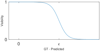
Figure 5: Soft visibility function. We plot $\|\mathbf{s}-\mathbf{x}\|-f_{\text{DDF}}(\mathbf{s},-\mathbf{d})$ on the $x$-axis versus $V(\mathbf{x},\mathbf{d})$ on the $y$-axis. When ground truth distance is significantly smaller than the threshold $\epsilon$, we assign a visibility of 1. When significantly larger, we infer an occlusion and a visibility of 0. In the vicinity of $\epsilon$ we smoothly transition from visible to non-visible with a steepness controlled by $s$.

Supervising the DDF    The DDF determines visibility which in turn determines appearance via the rendering equation in (1). This means that the DDF is partially supervised by the appearance loss. However, we also require that the DDF’s representation of scene geometry is consistent with the SDF geometry. We enforce this consistency through four losses. First, the depth predicted by the DDF should match that of the scene parameterised by the SDF:

$$\mathcal{L}_{\text{ddf\_depth}}=\sum_{(\mathbf{s},\mathbf{d})\in\mathcal{B}}w(\mathbf{d})\cdot|d_{\text{SDF}}(\mathbf{s},\mathbf{d})-f_{\text{DDF}}(\mathbf{s},\mathbf{d})|,$$ (5)

where $\mathcal{B}$ is a batch of positions on the sphere and inward facing directions. $d_{\text{SDF}}(\mathbf{s},\mathbf{d})$ is the ground truth expected termination depth for a ray from $\mathbf{s}$ in direction $\mathbf{d}$, computed from the current SDF. $w(\mathbf{r})$ is a weighting that encourages more accurate depth estimation at the centre of the scene. Second, travelling the distance predicted by the DDF should arrive at the SDF level set:

$$\mathcal{L}_{\text{ddf\_levelset}}=\sum_{(\mathbf{s},\mathbf{d})\in\mathcal{B}}f_{\text{SDF}}(\mathbf{s}+f_{\text{DDF}}(\mathbf{s},\mathbf{d})\mathbf{d})^{2}.$$ (6)

Third, we can impose multiview consistency on the DDF. Given an arbitrary starting point $\mathbf{s}_{1}$ and inward facing direction $\mathbf{d}_{1}$, we compute a termination point $\mathbf{x}_{1}=\mathbf{s}_{1}+f_{\text{DDF}}(\mathbf{s}_{1},\mathbf{d}_{1})\mathbf{d}_{1}$. Now, from an arbitrary second point $\mathbf{s}_{2}$, the predicted DDF depth towards $\mathbf{x}_{1}$ must be no greater than $\|\mathbf{x}_{1}-\mathbf{s}_{2}\|$, since $\mathbf{x}_{1}$ would occlude $\mathbf{s}_{2}$:

$$\mathcal{L}_{\text{ddf\_multiview}}=\!\!\!\!\!\!\!\sum_{(\mathbf{s}_{1},\mathbf{d}_{1},\mathbf{s}_{2})\in\mathcal{B}}\!\!\!\!\!\!\!\max\left(0,f_{\text{DDF}}(\mathbf{s}_{2},\mathbf{d}_{2})-\|\mathbf{x}_{1}-\mathbf{s}_{2}\|\right)^{2},$$ (7)

where $\mathbf{d}_{2}=(\mathbf{x}_{1}-\mathbf{s}_{2})/\|\mathbf{x}_{1}-\mathbf{s}_{2}\|$. Finally, we further take advantage of our sky segmentation maps as an additional constraint on our DDF. Rays that intersect the sky have no occlusions between the camera origin and our DDF sphere. Our DDF should therefore predict at least the distance to the camera origin for those intersecting rays:

$$\mathcal{L}_{\text{ddf\_sky}}=\sum_{\mathbf{r}\in\mathcal{R}\cap\mathcal{S}_{\text{sky}}}\max\left(0,\|\mathbf{o}-\mathbf{s}\|-f_{\text{DDF}}(\mathbf{s},-\mathbf{r})\right)$$ (8)

where $\mathbf{s}$ is the point where the ray intersects the DDF sphere and $\mathbf{o}$ the camera origin.

3.3 Implementation

We implement our method in Nerfstudio [35], building on top of NeuS-Facto [45]. We convert our CityScapes [11] segmentation masks into classes for sky, ground plane, foreground and transient objects (vehicles, vegetation, people etc). We sample ray batches only from non-transient pixels. We use a hash grid with $16$ levels, $2^{19}$ hash table size, $2$ features per entry and a course and fine resolution of $16$ and $2048$ respectively. Our SDF and albedo networks are both $2$-Layer $256$-Neuron MLPs. We initialise our SDF as a sphere with radius=$0.1$. We use the pre-trained RENI++ [16] model with a latent dimension $K=100$ and initialise latent codes as zeroes, corresponding to the mean environment provided by the RENI++ prior. We initialise the per-image illumination scale as $\gamma=1$.

Our visibility network is a FiLM-Conditioned [8] SIREN [32] with $5$-Layers and $256$-Neurons in both the FiLM Mapping Network and the main SIREN. We condition our network on positions on the sphere using the same dimensional hash grid as our SDF. We first map from position to a hashed latent, this latent is then provided to the FiLM mapping network to condition the model. As per Section 3.2 we normalise direction to a local coordinate frame and these directions are positionally encoded as per NeRF [25]. We use a sigmoid activation function scaled by the size of our scene bounds to ensure a depth prediction within the correct range. We generate samples for DDF supervision via our PyTorch re-implementation of fast von Mises-Fisher distribution sampling from Pinzón et al [27]. We used a concentration parameter of $20.0$ for the distribution and sampled $8$ positions and $128$ directions per batch exclusively from the upper hemisphere.

We optimise our Proposal Samplers, SDF/Albedo Field and DDF using Adam [19] optimisers with a Cosine Decay [23] schedule and 500-step ‘warm-up’ phase. Our loss is the sum of $\mathcal{L}_{\text{app}}$, $\mathcal{L}_{\text{prior}}$, $\mathcal{L}_{\text{sky}}$, the four DDF supervision losses and a proposal sampler interlevel loss as per Mip-NeRF 360 [3]. Our initial learning rates are $1\text{e}{-2}$, $1\text{e}{-3}$ and $1\text{e}{-4}$ respectively. Our RENI++ latent codes and the visibility threshold parameter use Adam [19] optimisers with an exponentially decaying learning rate which is initialised at $1\text{e}{-2}$ and $1\text{e}{-3}$ respectively.

Figure 6: Four views of the depth predicted by the Spherical DDF for Site 1 in the NeRF-OSR [29] dataset (see Figure 1). Cameras are placed on the unit sphere looking towards the origin. The DDF is trained concurrently with the scene representation and can capture high-frequency details required for accurate shadows.

Figure 7: Ambient occlusion and shadows from a point source computed from our soft visibility via the DDF.

4 Evaluation

We begin by qualitatively evaluating the output of our system components. Figure 6 illustrates that our spherical DDF is able to produce detailed depth maps via a single forward pass from arbitrary viewpoints. The geometry of the building and ground plane are well reconstructed. In Figure 7 we visualise the output of the visibility network in two different ways. On the left we average visibility over all directions, giving a good approximation to ambient occlusion. On the right we compute visibility for a single direction, producing a sharp shadow.

	Site 1			Site 2			Site 3
	PSNR $\uparrow$	MSE $\downarrow$		PSNR $\uparrow$	MSE $\downarrow$		PSNR $\uparrow$	MSE $\downarrow$
NeRF-OSR [29]	19.34	0.012		16.35	0.027		15.66	0.029
FEGR [39]	21.53	0.007		17.00	0.023		17.57	0.018
NeuSky (Ours)	22.50	0.005		16.66	0.023		18.31	0.016

Table 1: Outdoor scene relighting results on the NeRF-OSR relighting benchmark.

Figure 8: Comparion of albedo and normals produced by NeRF-OSR [29], FEGR [39] and our method. We produce much sharper albedo and normals than both prior works.

We evaluate NeuSky on the NeRF-OSR [29] relighting benchmark. The NeRF-OSR dataset consists of eight sites captured over multiple sessions each with differing illumination conditions along with Low Dynamic Range (LDR) ground truth environment maps. The relighting benchmark, in which the ground truth environment map from a session is used to relight the scene and the appearance error computed from a single viewpoint per session, for pixels within a provided mask, covers sites $1-3$. Since this environment map is LDR with over-saturated pixels around the sun, [29] first scale pixels $>0.95$ by $10$ to simulate HDR before fitting their SH illumination model. To benchmark NeuSky we chose to tackle a more challenging task and instead estimate our illumination environment from a single holdout image, a test image from another viewpoint of the scene during the same session. From the holdout viewpoint, we hold our model static and optimise only RENI++ latent codes and scale $\gamma$ for each holdout image. For this, we only optimise the appearance losses: $\mathcal{L}_{\text{eval\_illumination}}=\mathcal{L}_{\text{app}}+\!\!\!\sum_{\mathbf{r}\in\mathcal{R}\cap\mathcal{S}_{\text{sky}}}\!\!\!\varepsilon(\mathbf{c}_{\text{gt}}(\mathbf{r}),\mathbf{c}_{\text{sky}}(\mathbf{r}))$. We then position the camera in the test viewpoint and evaluate within the provided mask. Our results can be found in Table 1. Despite not seeing the full illumination environment we achieve better relighting performance than both NeRF-OSR [29] and FEGR [39] and produce models with significantly higher quality geometry and albedo as shown in Figure 8. As shown in Figure 9, NeuSky is capable of disentangling illumination, albedo and shading and our sky visibility network and RENI++ combine to produce sharp shadows. Further results are shown in Figure 1.

Figure 9: A render from each of the test scenes in NeRF-OSR [29]. Environment maps sampled from the estimated illumination of RENI++[16], albedo and normals are shown alongside the ground truth images. Our method accurately disentangles albedo, lighting and shadows whilst producing very high-quality geometry.

5 Conclusion

We have presented the first outdoor scene inverse rendering approach that incorporates a model of natural illumination, exploits direct sky pixel observations and can be trained end-to-end with a visibility model. This enables our model to reproduce accurate shadows, avoids shadow baking into albedo, allows shadows to constrain geometry and illumination and achieves superior reconstruction on the NeRF-OSR dataset beating [29] and [39] in the relighting benchmark. There are a number of limitations of our work, namely a high training GPU memory requirement when using large batches and at between 5-8 hours, our optimisation time is slow by modern neural field standards. The most obvious extension to our approach would be to use a more complex reflectance model and accompanying material parameters. For reflective surfaces, second bounce illumination becomes more significant. It is possible that a DDF could be used to speed up multibounce ray casting in this context.

Acknowledgments and Disclosure of Funding

This project was supported by travel funds from the Bavarian Research Alliance (BayIntAn FAU -2023-29). James Gardner was supported by the EPSRC Centre for Doctoral Training in Intelligent Games & Games Intelligence (IGGI) (EP/S022325/1).

Supplementary Material

Appendix A Introduction

Here we provide quantitative and qualitative ablations of our visibility network, include further implementation details of our method and demonstrate our method on the remaining NeRF-OSR [29] scenes.

Appendix B Ablation

Without Visibility Network

Figure 10: Whilst the majority of the training images for Site 3 in the NeRF-OSR dataset [29] show the front of the building in shadow. With our visibility network enabled our predicted albedo removes that shading along with shadows around the sign (a), at the joint between brick and plaster (b) and on the ground (c). Smaller cutouts show renderings with sky visibility on the left and without sky visibility on the right.

As shown in Figure 10, with our sky-visibility network enabled our model is better able to disentangle shading from albedo, particularly in scenes in which many of the images captured are shaded, namely Site 3 of the NeRF-OSR [29] dataset. This is further demonstrated quantitatively in the results shown in Table 2.

	Site 1			Site 2			Site 3
	PSNR $\uparrow$	MSE $\downarrow$		PSNR $\uparrow$	MSE $\downarrow$		PSNR $\uparrow$	MSE $\downarrow$
NeRF-OSR [29]	19.34	0.012		16.35	0.027		15.66	0.029
FEGR [39]	21.53	0.007		17.00	0.023		17.57	0.018
NeuSky	22.50	0.005		16.66	0.023		18.31	0.016
NeuSky (w/o sky visibility)	22.30	0.006		16.64	0.025		16.99	0.021

Table 2: Outdoor scene relighting results on the NeRF-OSR relighting benchmark. Not including the visibility network in our model results in worse performance due to the ambiguity between albedo and shading.

Shadows Informing Geometry

As shown in Figure 11, which shows a rendering of Site 1 looking behind any of the training cameras for that scene, to explain shadows seen during training geometry has formed outside the view of any training camera. This is a key advantage of training our differentiable sky visibility network concurrently with our scene representation.

Figure 11: Due to our differentiable sky visibility network being trained concurrently with our scene representation. Shadows can inform geometry outside of any training camera view frustum as highlighted in red.

Figure 12: Renders of four other scenes in NeRF-OSR [29]. Environment maps, sampled from the estimated illumination of RENI++[16], albedo and normals are shown alongside the ground truth images. Our method accurately disentangles albedo, lighting and shadows whilst producing very high-quality geometry.

Appendix C Implementation Details

During data pre-processing, we assume all cameras are looking towards the object of interest and align the average focus point of all cameras to be at the centre of our scene.

The weighting $w(\mathbf{r})$ applied in $\mathcal{L}_{\text{ddf\_depth}}$, see Section 3.2 in the main paper, is defined as $1.0-\left(\frac{\|\mathbf{p_{\text{term}}}(\mathbf{d})\|}{\text{radius}}\right)^{\sigma}$, with $\mathbf{p_{\text{term}}}(\mathbf{d})$ being the position of the termination point in direction $\mathbf{d}$ given the ground truth distance, radius being the predefined radius of the scene, and $\sigma$ being the exponent for the distance weight used to control sharpness of the weighting, set at $3.0$ for all experiments. This weighting encourages more accurate depth estimation at the centre of the scene.

As one of the classes in our CityScapes [11] segmentation masks is ground, we have an optional ground plane alignment loss that enforces consistency between the volume rendered normal and the world-up vector for rays inside that mask. We use the normal consistency loss from MonoSDF [46]:

$$\mathcal{L}_{\text{gp}}=\!\!\!\sum_{\mathbf{r}\in\mathcal{R}\cap\mathcal{S}_{\text{gp}}}\!\!\!\|N(\mathbf{r})-\mathbf{w}\|_{1}+\left\|1-N(\mathbf{r})^{\top}\mathbf{w}\right\|_{1}$$ (9)

Where $\mathcal{S}_{\text{gp}}$ is the set of ground plane pixels, $N(\mathbf{r})$ is the volume rendered normal for ray $\mathbf{r}$ and $\mathbf{w}$ is the world-up vector defined as $[0,0,1]$.

Appendix D Further Results and Videos

In Figure 12 we provide more renderings of our model fit to the remaining NeRF-OSR [29] scenes, demonstrating further our model’s ability to capture high-frequency geometric details, and accurately disentangle shading and albedo ambiguities. We encourage the reader to view the rendered videos on our project page demonstrating the multi-view and re-lighting capabilities of our model. In each video, we move the camera around the scene, once the camera comes to a stop we rotate the illumination environment to demonstrate the accurate shadow reproduction and relighting capabilities of our model. We also include videos of our Directional Distance Field (DDF) which we used for our sky visibility estimations and is trained concurrently with the scene representation. Each frame of this video is a single forward pass through our DDF which is able to produce the highly accurate depth maps required for accurate shadows.

References

- [1] Tristan Aumentado-Armstrong, Stavros Tsogkas, Sven Dickinson, and Allan D. Jepson. Representing 3D Shapes With Probabilistic Directed Distance Fields. In Proceedings of the IEEE/CVF Conference on Computer Vision and Pattern Recognition (CVPR), pages 19343–19354, June 2022.
- [2] Jonathan T. Barron and Jitendra Malik. Shape, Illumination, and Reflectance from Shading. TPAMI, 2015.
- [3] Jonathan T. Barron, Ben Mildenhall, Dor Verbin, Pratul P. Srinivasan, and Peter Hedman. Mip-NeRF 360: Unbounded Anti-Aliased Neural Radiance Fields. CVPR, 2022.
- [4] Sean Bell, Kavita Bala, and Noah Snavely. Intrinsic images in the wild. ACM Transactions on Graphics (TOG), 33(4):1–12, 2014.
- [5] Mark Boss, Varun Jampani, Raphael Braun, Ce Liu, Jonathan T. Barron, and Hendrik Lensch. Neural-PIL: Neural Pre-Integrated Lighting for Reflectance Decomposition. In A. Beygelzimer, Y. Dauphin, P. Liang, and J. Wortman Vaughan, editors, Advances in Neural Information Processing Systems, 2021.
- [6] Mark Boss, Varun Jampani, Kihwan Kim, Hendrik Lensch, and Jan Kautz. Two-shot spatially-varying brdf and shape estimation. In Proceedings of the IEEE/CVF Conference on Computer Vision and Pattern Recognition, pages 3982–3991, 2020.
- [7] Adrien Bousseau, Sylvain Paris, and Frédo Durand. User-assisted intrinsic images. In ACM SIGGRAPH Asia 2009 papers, pages 1–10. Association for Computing Machinery, New York, NY, United States, 2009.
- [8] Eric R. Chan, Marco Monteiro, Petr Kellnhofer, Jiajun Wu, and Gordon Wetzstein. Pi-GAN: Periodic Implicit Generative Adversarial Networks for 3D-Aware Image Synthesis. In Proceedings of the IEEE/CVF Conference on Computer Vision and Pattern Recognition (CVPR), pages 5799–5809, June 2021.
- [9] Zhe Chen, Yuchen Duan, Wenhai Wang, Junjun He, Tong Lu, Jifeng Dai, and Yu Qiao. Vision Transformer Adapter for Dense Predictions. In The Eleventh International Conference on Learning Representations, 2023.
- [10] Zhaoxi Chen, Guangcong Wang, and Ziwei Liu. Text2Light: Zero-Shot Text-Driven HDR Panorama Generation. ACM Trans. Graph., 41(6), Nov. 2022. Number of pages: 16 Place: New York, NY, USA Publisher: Association for Computing Machinery tex.articleno: 195 tex.issue_date: December 2022.
- [11] Marius Cordts, Mohamed Omran, Sebastian Ramos, Timo Rehfeld, Markus Enzweiler, Rodrigo Benenson, Uwe Franke, Stefan Roth, and Bernt Schiele. The Cityscapes Dataset for Semantic Urban Scene Understanding. In Proc. of the IEEE Conference on Computer Vision and Pattern Recognition (CVPR), 2016.
- [12] Mohammad Reza Karimi Dastjerdi, Yannick Hold-Geoffroy, Jonathan Eisenmann, and Jean-François Lalonde. EverLight: Indoor-Outdoor Editable HDR Lighting Estimation, 2023. arXiv: 2304.13207 [cs.CV].
- [13] Akshat Dave, Yongyi Zhao, and Ashok Veeraraghavan. PANDORA: Polarization-Aided Neural Decomposition of Radiance. In Shai Avidan, Gabriel J. Brostow, Moustapha Cissé, Giovanni Maria Farinella, and Tal Hassner, editors, Computer Vision - ECCV 2022 - 17th European Conference, Tel Aviv, Israel, October 23-27, 2022, Proceedings, Part VII, volume 13667 of Lecture Notes in Computer Science, pages 538–556. Springer, 2022. tex.bibsource: dblp computer science bibliography, https://dblp.org tex.biburl: https://dblp.org/rec/conf/eccv/DaveZV22.bib tex.timestamp: Mon, 05 Dec 2022 13:35:31 +0100.
- [14] Ron O. Dror, Alan S. Willsky, and Edward H. Adelson. Statistical characterization of real-world illumination. Journal of Vision, 4(9):11–11, Sept. 2004.
- [15] James A D Gardner, Bernhard Egger, and William A P Smith. Rotation-Equivariant Conditional Spherical Neural Fields for Learning a Natural Illumination Prior. In Alice H. Oh, Alekh Agarwal, Danielle Belgrave, and Kyunghyun Cho, editors, Advances in Neural Information Processing Systems, 2022.
- [16] James A. D. Gardner, Bernhard Egger, and William A. P. Smith. Reni++ a rotation-equivariant, scale-invariant, natural illumination prior, 2023.
- [17] Roger Grosse, Micah K Johnson, Edward H Adelson, and William T Freeman. Ground truth dataset and baseline evaluations for intrinsic image algorithms. In 2009 IEEE 12th International Conference on Computer Vision, pages 2335–2342. IEEE, 2009.
- [18] Jonathan Ho, Ajay Jain, and Pieter Abbeel. Denoising Diffusion Probabilistic Models. In H. Larochelle, M. Ranzato, R. Hadsell, M.F. Balcan, and H. Lin, editors, Advances in Neural Information Processing Systems, volume 33, pages 6840–6851. Curran Associates, Inc., 2020.
- [19] Diederik P. Kingma and Jimmy Ba. Adam: A Method for Stochastic Optimization. In Yoshua Bengio and Yann LeCun, editors, 3rd International Conference on Learning Representations, ICLR 2015, San Diego, CA, USA, May 7-9, 2015, Conference Track Proceedings, 2015. tex.bibsource: dblp computer science bibliography, https://dblp.org tex.timestamp: Thu, 25 Jul 2019 14:25:37 +0200.
- [20] Balazs Kovacs, Sean Bell, Noah Snavely, and Kavita Bala. Shading annotations in the wild. In Proceedings of the IEEE conference on computer vision and pattern recognition, pages 6998–7007, 2017.
- [21] Quewei Li, Jie Guo, Yang Fei, Feichao Li, and Yanwen Guo. NeuLighting: Neural Lighting for Free Viewpoint Outdoor Scene Relighting with Unconstrained Photo Collections. In SIGGRAPH Asia 2022 Conference Papers, SA ’22, New York, NY, USA, 2022. Association for Computing Machinery. Number of pages: 9 Place: Daegu, Republic of Korea tex.articleno: 13.
- [22] Zhuoman Liu, Bo Yang, Yan Luximon, Ajay Kumar, and Jinxi Li. RayDF: Neural Ray-surface Distance Fields with Multi-view Consistency. In Thirty-seventh Conference on Neural Information Processing Systems, 2023.
- [23] Ilya Loshchilov and Frank Hutter. SGDR: Stochastic Gradient Descent with Warm Restarts. In International Conference on Learning Representations, 2017.
- [24] Linjie Lyu, Marc Habermann, Lingjie Liu, Ayush Tewari, Christian Theobalt, et al. Efficient and differentiable shadow computation for inverse problems. In Proceedings of the IEEE/CVF International Conference on Computer Vision, pages 13107–13116, 2021.
- [25] Ben Mildenhall, Pratul P. Srinivasan, Matthew Tancik, Jonathan T. Barron, Ravi Ramamoorthi, and Ren Ng. NeRF: Representing Scenes as Neural Radiance Fields for View Synthesis. In ECCV, 2020.
- [26] Thomas Müller, Alex Evans, Christoph Schied, and Alexander Keller. Instant Neural Graphics Primitives with a Multiresolution Hash Encoding. ACM Trans. Graph., 41(4):102:1–102:15, July 2022. Number of pages: 15 Place: New York, NY, USA Publisher: ACM tex.articleno: 102 tex.issue_date: July 2022.
- [27] Carlos Pinzón and Kangsoo Jung. Fast Python sampler for the von Mises Fisher distribution. tex.hal_id: hal-04004568 tex.hal_version: v3, Aug. 2023.
- [28] Helge Rhodin, Nadia Robertini, Christian Richardt, Hans-Peter Seidel, and Christian Theobalt. A versatile scene model with differentiable visibility applied to generative pose estimation. In Proceedings of the 2015 International Conference on Computer Vision (ICCV 2015), 2015.
- [29] Viktor Rudnev, Mohamed Elgharib, William Smith, Lingjie Liu, Vladislav Golyanik, and Christian Theobalt. NeRF for Outdoor Scene Relighting. In European Conference on Computer Vision (ECCV), 2022.
- [30] Johannes Lutz Schönberger and Jan-Michael Frahm. Structure-from-motion revisited. In Conference on Computer Vision and Pattern Recognition (CVPR), 2016.
- [31] Johannes Lutz Schönberger, Enliang Zheng, Marc Pollefeys, and Jan-Michael Frahm. Pixelwise view selection for unstructured multi-view stereo. In European Conference on Computer Vision (ECCV), 2016.
- [32] Vincent Sitzmann, Julien N.P. Martel, Alexander W. Bergman, David B. Lindell, and Gordon Wetzstein. Implicit Neural Representations with Periodic Activation Functions. In Proc. NeurIPS, 2020.
- [33] Gowri Somanath and Daniel Kurz. Hdr environment map estimation for real-time augmented reality. In Proceedings of the IEEE/CVF Conference on Computer Vision and Pattern Recognition (CVPR), pages 11298–11306, June 2021.
- [34] Pratul P. Srinivasan, Boyang Deng, Xiuming Zhang, Matthew Tancik, Ben Mildenhall, and Jonathan T. Barron. NeRV: Neural Reflectance and Visibility Fields for Relighting and View Synthesis. In Proceedings of the IEEE/CVF Conference on Computer Vision and Pattern Recognition (CVPR), pages 7495–7504, June 2021.
- [35] Matthew Tancik, Ethan Weber, Evonne Ng, Ruilong Li, Brent Yi, Justin Kerr, Terrance Wang, Alexander Kristoffersen, Jake Austin, Kamyar Salahi, Abhik Ahuja, David McAllister, and Angjoo Kanazawa. Nerfstudio: A Modular Framework for Neural Radiance Field Development. arXiv preprint arXiv:2302.04264, 2023.
- [36] Itsuki Ueda, Yoshihiro Fukuhara, Hirokatsu Kataoka, Hiroaki Aizawa, Hidehiko Shishido, and Itaru Kitahara. Neural Density-Distance Fields. In Proceedings of the European Conference on Computer Vision, 2022.
- [37] Peng Wang, Lingjie Liu, Yuan Liu, Christian Theobalt, Taku Komura, and Wenping Wang. NeuS: Learning Neural Implicit Surfaces by Volume Rendering for Multi-view Reconstruction. In A. Beygelzimer, Y. Dauphin, P. Liang, and J. Wortman Vaughan, editors, Advances in Neural Information Processing Systems, 2021.
- [38] Peng Wang, Lingjie Liu, Yuan Liu, Christian Theobalt, Taku Komura, and Wenping Wang. NeuS: Learning Neural Implicit Surfaces by Volume Rendering for Multi-view Reconstruction. In A. Beygelzimer, Y. Dauphin, P. Liang, and J. Wortman Vaughan, editors, Advances in Neural Information Processing Systems, 2021.
- [39] Zian Wang, Tianchang Shen, Jun Gao, Shengyu Huang, Jacob Munkberg, Jon Hasselgren, Zan Gojcic, Wenzheng Chen, and Sanja Fidler. Neural Fields meet Explicit Geometric Representations for Inverse Rendering of Urban Scenes. In The IEEE Conference on Computer Vision and Pattern Recognition (CVPR), June 2023.
- [40] Lance Williams. Casting curved shadows on curved surfaces. In Proceedings of the 5th annual conference on Computer graphics and interactive techniques, pages 270–274, 1978.
- [41] Markus Worchel and Marc Alexa. Differentiable shadow mapping for efficient inverse graphics. In Proceedings of the IEEE/CVF Conference on Computer Vision and Pattern Recognition, pages 142–153, 2023.
- [42] Yao Yao, Jingyang Zhang, Jingbo Liu, Yihang Qu, Tian Fang, David McKinnon, Yanghai Tsin, and Long Quan. NeILF: Neural Incident Light Field for Physically-based Material Estimation. In Shai Avidan, Gabriel Brostow, Moustapha Cissé, Giovanni Maria Farinella, and Tal Hassner, editors, Computer Vision – ECCV 2022, pages 700–716, Cham, 2022. Springer Nature Switzerland.
- [43] Tarun Yenamandra, Ayush Tewari, Nan Yang, Florian Bernard, Christian Theobalt, and Daniel Cremers. FIRe: Fast Inverse Rendering using Directional and Signed Distance Functions, 2022. arXiv: 2203.16284 [cs.CV].
- [44] Ye Yu and William A. P. Smith. InverseRenderNet: Learning Single Image Inverse Rendering. In Proceedings of the IEEE/CVF Conference on Computer Vision and Pattern Recognition (CVPR), June 2019.
- [45] Zehao Yu, Anpei Chen, Bozidar Antic, Songyou Peng Peng, Apratim Bhattacharyya, Michael Niemeyer, Siyu Tang, Torsten Sattler, and Andreas Geiger. SDFStudio: A Unified Framework for Surface Reconstruction, 2022.
- [46] Zehao Yu, Songyou Peng, Michael Niemeyer, Torsten Sattler, and Andreas Geiger. MonoSDF: Exploring Monocular Geometric Cues for Neural Implicit Surface Reconstruction. In S. Koyejo, S. Mohamed, A. Agarwal, D. Belgrave, K. Cho, and A. Oh, editors, Advances in Neural Information Processing Systems, volume 35, pages 25018–25032. Curran Associates, Inc., 2022.
- [47] Kai Zhang, Fujun Luan, Qianqian Wang, Kavita Bala, and Noah Snavely. Physg: Inverse rendering with spherical gaussians for physics-based material editing and relighting. In Proceedings of the IEEE/CVF Conference on Computer Vision and Pattern Recognition, pages 5453–5462, 2021.
- [48] Xiuming Zhang, Pratul P. Srinivasan, Boyang Deng, Paul Debevec, William T. Freeman, and Jonathan T. Barron. NeRFactor: Neural Factorization of Shape and Reflectance under an Unknown Illumination. ACM Trans. Graph., 40(6), Dec. 2021. Number of pages: 18 Place: New York, NY, USA Publisher: Association for Computing Machinery tex.articleno: 237 tex.issue_date: December 2021.
- [49] Pierre Zins, Yuanlu Xu, Edmond Boyer, Stefanie Wuhrer, and Tony Tung. Multi-View Reconstruction using Signed Ray Distance Functions (SRDF), 2023. arXiv: 2209.00082 [cs.CV].
- [50] Ehsan Zobeidi and Nikolay Atanasov. A Deep Signed Directional Distance Function for Object Shape Representation. CoRR, abs/2107.11024, 2021. arXiv: 2107.11024 tex.bibsource: dblp computer science bibliography, https://dblp.org tex.timestamp: Fri, 04 Aug 2023 08:25:46 +0200.