Universality in Ground State Masses of Nuclei

Abstract

The beautiful and profound result that the first eigenvalue of Schrödinger operator can be interpreted as a large deviation of certain kind of Brownian motion leads to possible existence of universality in the distribution of ground state energies of quantal systems. Existence of such universality is explored in the distribution of the ground state energies of nuclei with $Z\geq 8$ and $N\geq 8$. Specifically, it has been demonstrated that the nuclear masses follow extreme-value statistics, implying that the nuclear ground state energies indeed can be treated as extreme values in the sense of the large deviation theory of Donsker and Varadhan.

1 Introduction

A glimpse at the energy levels of nuclei reveals their complexity: the “bar codes” seem to bear similarity at a gross level with some nuclei showing more clustering than others. Larger clustering is related to degeneracies and well-known magic numbers in nuclei bm and metallic clusters brack , with origin in underlying symmetries. Energy level patterns are characterized at a gross level in terms of mean density, epitomized in Thomas-Fermi and other semiclassical formulae. A closer look brings out fluctuation properties which correlate densities at two or more energies ap ; guhr ; kota . In the scaling limit, the level correlations have been successfully explained by Random Matrix Theory (RMT). However, at the centre of the physics of nuclei resides the ground states and the corresponding nuclear masses. Here we address “the elephant at the centre” and present a compelling case for universality associated with ground state energies. Its origin is in our consideration of ground state (GS) energies as extreme values comment of the spectra. The collection of these extreme values, taken for all nuclei, constitutes an ensemble, named as ground state ensemble (gSE).

The GS corresponds to the first eigenvalue of the self-adjoint operator, which is calculated by setting up a variational formulation leading to the Rayleigh - Ritz formula. Ground state energy for a Hamiltonian operator may also be calculated by employing the Feynman - Kac formula which is based on the asymptotic form of the Green function. It turns out that the first eigenvalue of the Schrödinger operator can be interpreted as a large deviation of certain kind of a Brownian motion. Donsker and Varadhan generalized this variational formulation to what they call the principal eigenvalue (GS in our nomenclature) for operators with maximum principle dv , thus providing a large-deviation interpretation of variational formula which reduces to the Rayleigh - Ritz formula for self-adjoint operators. This beautiful work is at the basis of our result.

2 Computational Details and Results

The goal of this work is to establish the universality argued above, which is associated with the ground state energies of nuclei quantitatively. For this purpose, we choose nuclei with atomic number, $Z\geq 8$ and neutron number, $N\geq 8$. For all 2353 nuclei, experimental masses have been considered from the atomic mass evaluation of 2012 WAN.12a ; WAN.12b . The fluctuations in the ground state energies can be obtained by subtracting the liquid drop binding energies ($E_{\rm LDM}$) from the experimental binding energies. This procedure is justified, and can be argued to be robust, since it is well known that all the variants of the liquid drop model yield binding energies that are similar to each other. Thus, the general conclusions drawn are not sensitive to a particular choice of the liquid drop model. Here, we consider a liquid drop model POM.03 ; BHA.12a ; BHA.12b ; BHA.21 with binding energy $E_{LDM}$ (see Appendix A for details).

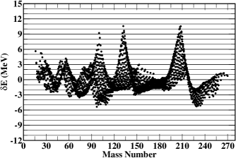
Figure 1: Difference between experimental and LDM binding energies. These are sharply peaked at the magic nuclei such as ${}^{100,132}Sn$ and ²⁰⁸Pb.

We denote the difference between experimental energies and $E_{LDM}$ by $\delta E$, and it is this quantity that we shall be analysing further to investigate the universality associated with the ground state energies. Here, we adopt the sign convention where the quantity $\delta E$ is positive at shell closures. Notice that the LDM assumed above does not have any deformation dependence, nor it contains any terms such as the Wigner correction. The only effect that has been taken in addition to the usual ‘macroscopic’ terms is the pairing energy. This is justified again on the basis of an idea similar to the Strutinsky theorem: exactly like the binding energy (barring two - body correlations), the pairing energy can be thought to be made of a ‘smooth’ part and a fluctuating part VIN.11 .

The quantity $\delta E$ is plotted in Fig. (1) for the chosen set of 2353 nuclei as a function of mass number. It can be seen that the sharp peaks are observed precisely at the locations of doubly magic nuclei. The mean of $\delta E$ turns out to be nearly zero. The plot also hints towards the possible choice of bin size for statistical study of this data set: an inspection of the graph suggests a bin size of about 1 MeV. For reliable conclusions, the bin size has to be optimal, the analysis of which we come to now. The question of optimality can be answered by a binning method developed by Shimazaki and Shinomoto SHI.07 . The idea is to choose the bin size such that the cost function is minimized, the details of this well-known procedure are explained in Appendix B.

Using the present data, Shimazaki-Shinomoto procedure gives an optimal bin-width to be $h\sim 1$ MeV.

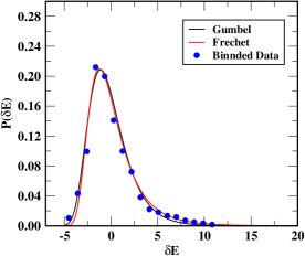
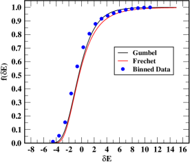
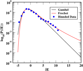
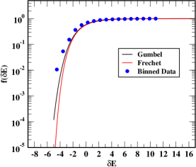
Figure 2: The probability distribution $P(\delta E)$ obtained from binning procedure as a function of $\delta E$. Fits to the Gumbel and Fréchet distributions and cumulative distributions on linear as well as $\log$ scale are shown.

The resulting frequency distribution, normalized to unity, is plotted in Fig. 2. The distribution is clearly different from Gaussian. In the light of the argument suggesting the possibility of the distribution being one of the extreme-value distributions (GEV), we first check if the distribution is a Gumbel distribution, expressed as:

$$P\left(x\right)=\frac{1}{\beta}\exp\left\{-\frac{\left(x-\mu\right)}{\beta}-\exp\left[-\frac{\left(x-\mu\right)}{\beta}\right]\right\}$$ (1)

where the scale parameter $\beta\in\mathbb{R}^{+}$ and the location parameter $\mu\in\mathbb{R}$. The support of this distribution is the whole of $\mathbb{R}$, i.e., $x\in\mathbb{R}$. The cumulative distribution function is expressed as:

$$f\left(x\right)=\exp\left\{-\exp\left[-\frac{\left(x-\mu\right)}{\beta}\right]\right\}.$$ (2)

The parameters $\mu$ and $\beta$ in this work are obtained through $\chi^{2}$ minimisation, using the well-known Powell’s conjugate direction method POW.64 , which is a derivative - free optimization technique for finding local minima of a given function. The values of the parameters thus obtained are $\mu$ = -1.12445 and $\beta$ = 1.78709. The fit turns out to be good, with an r.m.s. deviation of 1.4$\times 10^{-4}$.

The observation recorded above needs to be substantiated further. In order to do that, we consider the general GEV distribution:

$$P\left(x\right) = \frac{1}{\beta}\left\{1+\xi\left(\frac{x-\mu}{\beta}\right)\right\}^{-\left(1+\xi\right)/\xi}\times$$ (3)

$$\hskip 48.0pt\exp{\left\{1+\xi\left(\frac{x-\mu}{\beta}\right)\right\}^{-1/\xi}}$$

If $\xi$ = 0, we get the Gumbel distribution and the corresponding support is $\mathbb{R}$. On the other hand, if $\xi<0$, one obtains the Weibull distribution, with the support that is bounded above, that is, with $x\in\left(-\infty\right.,\left.\mu-\beta/\xi\right]$. Finally, if $\xi>0$, the Fréchet distribution is obtained, with the support that is bounded below, such that $x\in\left[\mu-\beta/\xi\right.,\left.\infty\right)$. The cumulative distribution function in the case of GEV is expressed as:

$$f\left(x\right)=\exp\left\{1+\xi\left(\frac{x-\mu}{\beta}\right)\right\}^{-1/\xi}$$ (4)

The parameters are determined using Powell’s method. The explicit values of the parameters are: $\mu$ = -1.03173, $\beta$ = 1.79009 and $\xi$ = 0.13552 with rms deviation of 1.2$\times 10^{-4}$. The fact that $\xi>0$ indicates that this is a Fréchet distribution.

3 Statistical Analysis

On the face of it, it seems that we have fitted the same data equally well with two different probability densities. However, we shall now establish that the two seemingly different distributions are statistically indistinguishable. To begin with, notice that the values of the position and scale parameters in the two cases are very close to each other: the position parameters differ by about 5%, whereas the scale parameters differ by less than 0.2%. Secondly, the value of the shape parameter is just about 0.14 which is quite small indeed. The lower bound on the support works out to be $\sim$-14, which is very large and negative (notice that the smallest value of $\delta E$ in this data set is $\sim$-4.5). Thus, it is to be expected a priori that the two should be almost identical, particularly so far as shapes are concerned. This observation is amply reflected in Fig. (3), where, we plot the two probability distributions and cumulative distributions along with the corresponding binned data. It is clear from the graph that the two distributions are very close to each other, and also describe the binned data very well. The cumulative distribution however shows that there are differences between Gumbel and Fréchet, and we shall quantify them here.

To quantify this near-indistinguishability of the two distributions, one sample Kolmogorov-Smirnov test (see, for example, DOD.08 ) is carried out to test the null hypothesis that the fitted Gumbel and Fréchet empirical data (cumulative probability at the midpoint of a bin) is identical to the one for Gumbel distribution (Eqs. (1) and (2)). The former is denoted by $S_{n}(x)$ and the latter by $f(x)$. Then the Chebyshev norm,

$$D=\max_{x\in\mathbb{R}}\left|S_{n}(x)-f(x)\right|,\quad n\in\mathbb{N}$$ (5)

gives the Kolmogorov - Smirnov statistic. Let the significance level of an observed value of $D$ be denoted by $P$. small values of $P$ show that the cumulative distribution function $S_{n}$ is significantly different from the hypothesised function, $f(x)$ (for details, refer to DOD.08 ; NR.92 ). In other words, the null hypothesis that the two are the same is to be accepted if the $P$ value is close to 1. In the present case, $D$ turns out to be equal to 1.5$\times 10^{-2}$, leading to $P\sim 1$, confirming the null hypothesis. We now perform the Kolmogorov - Smirnov test once again for the cumulative distributions. Even in this case, the quantity $D$ works out to be 3.3$\times 10^{-2}$, leading to $P\sim 0.98$, supporting the above conclusion. From these two conclusions alone, one may conclude that within the Kolmogorov - Smirnov criteria, the two distributions are almost identical.

We now test the closeness of the ‘observed’ distribution (binned data) to the fitted Gumbel distribution. The null hypothesis, in this case, is that the empirical data (probability at the midpoint of a bin) is identical to the one for that of the Gumbel distribution. Again, the infinity norm ($D$) turns out to be $\sim$0.1, leading to $P\sim 0.99$, validating the null hypothesis. As we had done earlier, we now apply the Kolmogorov - Smirnov test to the cumulative distributions. In that case, $D$ works out to be $\sim$0.11, leading to $P\sim 0.99$, substantiating the claim that indeed, the distribution is a Gumbel distribution as per the Kolmogorov - Smirnov test.

We next compute the quantities, mean ($E[X]$), variance ($\mathrm{Var}(x)$), skewness ($\tilde{\mu}_{3}$), excess kurtosis (${\cal{K}}[X]$) and Shannon entropy ($H(X)$), characterising the Gumbel and Fréchet distribution, as well as the binned data. The explicit expressions for these quantities are summarised in Appendix C.

Table 1: Various quantities characterising the probability distributions. Here the quantities listed under ‘Binned Data’ stand for those computed directly from the binned data, ‘Exact’ means the ones calculated from the exact expressions for all the relevant quantities (detailed in Appendix C), and ‘Bin Centroid’ implies the quantities computed by taking $\delta E$ to be the bin centroid.

		From Distribution
		Gumbel		Fréchet
Quantity	Binned Data	Exact	Bin Centroid	Exact	Bin Centroid
$E[X]$	0.003	-0.099	-0.111	0.222	0.152
Var$(X)$	6.319	5.112	5.218	7.475	6.454
$\tilde{\mu}_{3}$	1.269	1.140	1.038	2.140	1.310
${\cal{K}}[X]$	2.144	2.4	1.568	10.549	2.195
$H(X)$	2.247	2.144	2.228	2.215	2.270

A comparison between these quantities (denoted by ‘From Distribution’) and the corresponding quantities computed directly from binned data (denoted by ‘Binned Data’) is made in Table (1). In addition, the quantities computed by using the exact distribution functions, but only the bin centroids are also presented there. By and large, these agree with each other reasonably well. The only exception is excess kurtosis, which has been grossly underestimated for the Fréchet distribution. The binned data, exact result for Gumbel, and kurtosis obtained for Fréchet from centroids are quite close to each other, whereas the exact result for Fréchet is way too high: this is to be expected, as can be seen from the plot where the distributions have been presented on log scale: the Fréchet distribution tends to have a rather heavy tail, and this dominates kurtosis: it is well known that it is both the peak and tail that contribute to kurtosis (see, for example, DEC.97 ). Fréchet has a rather heavy tail, and while computing the kurtosis from bin centroids (with exact distribution), the tail has not been fully accounted for.

4 Discussion and Summary

The distribution of $\delta E$ is a GEV. As per the Kolmogorov - Smirnov test, as well as the visual confirmation that we get after examining the two distributions along with the binned data, it is apparent that the Gumbel and Fréchet distributions here behave alike, given that the parameter $\xi$ is small: it is a well known fact that in the limit of $\xi\rightarrow 0$, Fréchet distribution ‘tends’ to Gumbel. Thus, so far as these measures are concerned, the two are almost identical, and the distribution can be safely taken to be a Gumbel distribution. This is further supported by the observation that the excess kurtosis value of the binned data is very similar to that of the Gumbel distribution. Even the excess kurtosis obtained by assuming exact Gumbel distribution and centroids of the bins yields an excess kurtosis that is not too far from these two. Fréchet distribution, on the other hand, has a very large excess kurtosis, which does not really agree with the other calculations. The excess kurtosis obtained from bin centroids is closer to the others, but this is primarily due to the fact that the entire distribution is not taken into account here.

Whereas the energy levels of nuclei are known to possess correlations which are well-understood in terms of RMT ap ; bhp , we have argued that the ground state energies may be treated as extreme values in the sense of large-deviations theory. This is not only interesting but also significant as we are able to propose a universality for nuclear masses which happens to belong to one of the well-known distributions. We would like to emphasize that the kernel of the argument leading to our finding is in the profound work by Donsker and Varadhan dv .

Appendix A Liquid Drop Model

Here, we consider a liquid drop model inspired from Pomorski’s work POM.03 ; BHA.12a ; BHA.12b ; BHA.21 ; BHA.14 , expressed as

$$E_{LDM} = a_{v}\left[1~{}+~{}\frac{4k_{v}}{A^{2}}~{}T_{z}\left(T_{z}~{}+~{}1\right)\right]A$$ (6)

$$+ a_{s}\left[1~{}+~{}\frac{4k_{s}}{A^{2}}~{}T_{z}\left(T_{z}~{}+~{}1\right)\right]A^{2/3}$$

$$+ \frac{3Z^{2}e^{2}}{5r_{0}A^{1/3}}~{}+~{}\frac{C_{4}Z^{2}}{A}~{}+~{}E_{p}.$$

In this expression, $T_{z}$ is the third component of isospin and $e$ is the electronic charge. The coefficients $a_{v}$, $k_{v}$, $a_{s}$, $k_{s}$, $r_{0}$ and $C_{4}$ (correction to Coulomb energy due to surface diffuseness) are treated to be free parameters. Following Möller and Nix NIX.92 , the smooth pairing energy is assumed to be of the form

$$E_{p} = \frac{d_{n}}{N^{1/3}}~{},~{}\mathrm{for}~{}N~{}\mathrm{odd~{}and~{}}Z\mathrm{~{}even}$$ (7)

$$= \frac{d_{p}}{Z^{1/3}}~{},~{}\mathrm{for}~{}Z~{}\mathrm{odd~{}and~{}}N\mathrm{~{}even}$$

$$= \frac{d_{n}}{N^{1/3}}+\frac{d_{p}}{Z^{1/3}}+\frac{d_{np}}{A^{2/3}}~{},~{}\mathrm{for}~{}Z~{}\mathrm{and~{}}N\mathrm{~{}odd}$$

$$= 0~{},~{}\mathrm{for}~{}Z~{}\mathrm{and~{}}N\mathrm{~{}even}.$$

with the constants $d_{n}$, $d_{p}$ and $d_{np}$ being free parameters. These parameters have been determined through $\chi^{2}$ - minimisation through the NETLIB NETLIB implementation of the Levenberg - Marquardt (LM) algorithm MAR.68 ; KEL.99 . The values of the coefficients thus obtained are BHA.14 : $a_{v}$ = -15.505 MeV; $a_{s}$ = 17.830 MeV; $k_{v}$ = -1.825; $k_{s}$ = -2.265; $r_{0}$ = 1.215 fm; $C_{4}$ = 1.297 MeV; $d_{n}$ = 4.687 MeV; $d_{p}$ = 4.717 MeV; and $d_{np}$ = -6.495 MeV. The rms deviation obtained for the fit, as expected MYE.96 , is 2.456 MeV.

Appendix B Optimisation of Bin-size

Suppose, that for given width $\Delta$, there are $M$ bins in all. Let $n_{k}$ represent number of objects in the $k^{th}$ bin. Then, the mean $\bar{n}$ and variance $v$ corresponding to the data are defined by obvious expressions SHI.07

$$\bar{n}=\frac{1}{M}\sum_{j=1}^{M}n_{k},\qquad v=\frac{1}{M}\sum_{j=1}^{M}\left(n_{k}-\bar{n}\right)^{2}.$$ (8)

Given these quantities, the cost function, which depends explicitly on the bin width, is given by SHI.07

$$C\left(\Delta\right)=\frac{2\bar{n}-v}{\Delta^{2}}.$$ (9)

The Shimazaki-Shinomoto procedure amounts to determination of $\Delta$ such that the above cost function is minimized.

Appendix C Gumbel and Fréchet distribution

Quantities calculated for Gumbel and Fréchet distribution, as well as for the binned data are detailed here: mean ($E[X]$), variance ($\mathrm{Var}(x)$), skewness ($\tilde{\mu}_{3}$), excess kurtosis (${\cal{K}}[X]$) and Shannon entropy ($H(X)$). These quantities can be computed exactly for a Gumbel as well as a Fréchet distribution (see, for example, FIN.03 for further details). We first list these quantities for a Gumbel distribution:

$$E[X] = \mu+\beta\gamma$$ (10)

$$\mathrm{Var}(X) = \frac{\pi^{2}}{6}\beta^{2}$$ (11)

$$\tilde{\mu}_{3} = \frac{12\sqrt{6}\,\zeta\left(3\right)}{\pi^{3}}$$ (12)

$${\cal{K}}[X] = \frac{12}{5}$$ (13)

$$H(X) = \log\left(\beta\right)+\gamma+1$$ (14)

where, $\zeta\left(3\right)$ is the Riemann zeta function with argument 3, also known as the Apéry’s constant and $\gamma$ is the Euler - Mascheroni constant. On the other hand, these quantities for a Fréchet distribution are given by:

$$E[X] = \mu+\beta\frac{\left({\cal{G}}_{1}\!\left(\xi\right)-1\right)}{\xi}$$ (15)

$$\mathrm{Var}(X) = \beta^{2}\,\frac{{\cal{G}}_{2}\!\left(\xi\right)-{\cal{G}}_{1}\!\left(\xi\right)^{2}}{\xi^{2}}$$ (16)

$$\tilde{\mu}_{3} = \frac{{\cal{G}}_{3}\!\left(\xi\right)-3\,{\cal{G}}_{1}\!\left(\xi\right){\cal{G}}_{2}\!\left(\xi\right)+2\,{\cal{G}}_{1}\!\left(\xi\right)^{3}}{\left({\cal{G}}_{2}\!\left(\xi\right)-{\cal{G}}_{1}\!\left(\xi\right)^{2}\right)^{3/2}}$$ (17)

$${\cal{K}}[X] = \frac{{\cal{G}}_{4}\!\left(\xi\right)-4\,{\cal{G}}_{3}\!\left(\xi\right){\cal{G}}_{1}\!\left(\xi\right)-3\,{\cal{G}}_{2}\!\left(\xi\right)^{2}}{\left({\cal{G}}_{2}\!\left(\xi\right)-{\cal{G}}_{1}\!\left(\xi\right)^{2}\right)^{2}}$$ (18)

$$+ \frac{\left(\xi\right)^{2}{\cal{G}}_{2}\!\left(\xi\right)-6\,{\cal{G}}_{1}\!\left(\xi\right)^{4}}{\left({\cal{G}}_{2}\!\left(\xi\right)-{\cal{G}}_{1}\!\left(\xi\right)^{2}\right)^{2}}$$

$$H(X) = \log\left(\beta\right)+\gamma\left(\xi+1\right)+1$$ (19)

here, ${\cal{G}}_{k}\!\left(\xi\right)=\Gamma\left(1-k\xi\right)$, with $k\in\mathbb{N}$ and $\Gamma$ is the gamma function.

These quantities are computed by using the following expressions for the binned data:

$$E[X] = \sum_{n=1}^{N}x_{n}P\left(x_{n}\right)$$ (20)

$$\mathrm{Var}(X) = E\left[\left(X-E\left(X\right)\right)^{2}\right]$$ (21)

$$\tilde{\mu}_{3} = \frac{E\left[\left(X-E\left(X\right)\right)^{3}\right]}{\left\{E\left[\left(X-E\left(X\right)\right)^{2}\right]\right\}^{3/2}}$$ (22)

$${\cal{K}}[X] = \frac{E\left[\left(X-E\left(X\right)\right)^{4}\right]}{\left\{E\left[\left(X-E\left(X\right)\right)^{2}\right]\right\}^{2}}-3$$ (23)

$$H(X) = E\left[-\log\left(P\left(X\right)\right)\right]$$ (24)

References

- (1) A. Bohr and B. R. Mottelson, Nuclear Structure, W. A. Benjamin, Inc., New York (1969).
- (2) M. Brack, The physics of simple metal clusters: self-consistent jellium model and semiclassical approaches, Rev. Mod. Phys. 65 (1993) 677.
- (3) T. A. Brody, J. Flores, J. B. French, P. A. Mello, A. Pandey, and S. S. M. Wong, Random-matrix physics: spectrum and strength fluctuations, Rev. Mod. Phys. 53 (1981) 385.
- (4) T. Guhr, Axel Müller-Groeling, and H. A. Weidenmüller, Random-matrix theories in quantum physics: common concepts, Phys. Rep. 299 (1998) 189.
- (5) V. K. B. Kota, Embedded random matrix ensembles in quantum physics, Springer, Heidelberg (2014).
- (6) GS energies are of course the minima of the spectral sequence, these are the most extreme values. The point we are trying to make in the present work may also be taken as an argument which allows us to treat GS energies as extreme values, in the sense of statistics.
- (7) M. D. Donsker and S. R. S. Varadhan, On a Variational Formula for the Principal Eigenvalue for Operators with Maximum Principle, Proc. Natl Acad. Sc. (NY) 72 (1975) 780.
- (8) M. Wang, A.H. Wapstra, F.G. Kondev, M. MacCormick, X. Xu and B. Pfeiffer. The AME2012 atomic mass evaluation (I), Evaluation of input data, adjustment procedures, Chinese Phys. C 36 (2012) 1287.
- (9) M. Wang, G. Audi, A. H. Wapstra, F. G. Kondev, M. MacCormick, X. Xu and B. Pfeiffer, The Ame2012 atomic mass evaluation, Chinese Phys. C 36 (2012) 1603.
- (10) K. Pomorski and J. Dudek, Nuclear liquid-drop model and surface-curvature effects, Phys. Rev. C 67 (2003) 044316.
- (11) A. Bhagwat, X. Viñas, M. Centelles, P. Schuck and R. Wyss, Microscopic-macroscopic approach for binding energies with the Wigner-Kirkwood method, Phys. Rev. C 81 (2010) 044321.
- (12) A. Bhagwat, X. Viñas, M. Centelles, P. Schuck and R. Wyss, Microscopic-macroscopic approach for binding energies with the Wigner-Kirkwood method. II. Deformed nuclei, Phys. Rev. C 86 (2012) 044316.
- (13) A. Bhagwat, M. Centelles, X. Viñas, and P. Schuck, Microscopic-macroscopic approach for ground-state energies based on the Gogny force with the Wigner-Kirkwood averaging scheme, Phys. Rev. C 103 (2021) 024321.
- (14) X. Viñas, P. Schuck and M. Farine, Semiclassical Description of Average Pairing Properties in Nuclei, Int. J. Mod. Phys. E 20 (2011) 399.
- (15) H. Shimazaki and S. Shinomoto, A Method for Selecting the Bin Size of a Time Histogram, Neural Computation 19 (2007) 1503.
- (16) M. J. D. Powell, An efficient method for finding the minimum of a function of several variables without calculating derivatives, Computer Journal 7 (1964) 155.
- (17) Yadolah Dodge, The Concise Encyclopedia of Statistics, Springer, New York (2008), p. 283.
- (18) W. T. Vetterling, W. H. Press, S. A. Teukolsky and B. P. Flannery, Numerical Recipes in FORTRAN, 2nd Edition, Cambridge University Press, (1992), page 617ff.
- (19) L. T. DeCarlo, On the Meaning and Use of Kurtosis, Psych. Meth. 2 (1997) 292.
- (20) R. U. Haq, A. Pandey, and O. Bohigas, Fluctuation Properties of Nuclear Energy Levels: Do Theory and Experiment Agree?, Phys. Rev. Lett. 48 (1982) 1086.
- (21) P. Möller and J. R. Nix, Nuclear pairing models, Nucl. Phys. A536 (1992) 20.
- (22) D. W. Marquardt, An Algorithm for Least-Squares Estimation of Nonlinear Parameters, J. Soc. Ind. Appl. Math. 11 (1963) 431.
- (23) C. T. Kelley, Iterative Methods for Optimisation, Society for Industrial and Applied Mathematics, Philadelphia (1999).
- (24) E. Anderson, Z. Bai, C. Bischof, S. Blackford, J. Demmel, J. Dongarra, J. Du Croz, A. Greenbaum, S. Hammarling, A. McKenney and D. Sorensen, LAPACK User’s Guide, 3rd Edition, Society for Industrial and Applied Mathematics, Philadelphia (1999).
- (25) A. Bhagwat, Phys. Rev. C, 90 (2014) 064306.
- (26) W. D. Myers and W. J. Swiatecki, Nuclear properties according to the Thomas-Fermi model, Nucl. Phys. A601 (1996) 141.
- (27) Steven Finch, Mathematical Constants, Cambridge University Press, (2003), pages 363 - 367, and references cited therein.