Stein Variational Belief Propagation for Multi-Robot Coordination

Abstract

Decentralized coordination for multi-robot systems involves planning in challenging, high-dimensional spaces. The planning problem is particularly challenging in the presence of obstacles and different sources of uncertainty such as inaccurate dynamic models and sensor noise. In this paper, we introduce Stein Variational Belief Propagation (SVBP), a novel algorithm for performing inference over nonparametric marginal distributions of nodes in a graph. We apply SVBP to multi-robot coordination by modelling a robot swarm as a graphical model and performing inference for each robot. We demonstrate our algorithm on a simulated multi-robot perception task, and on a multi-robot planning task within a Model-Predictive Control (MPC) framework, on both simulated and real-world mobile robots. Our experiments show that SVBP represents multi-modal distributions better than sampling-based or Gaussian baselines, resulting in improved performance on perception and planning tasks. Furthermore, we show that SVBP’s ability to represent diverse trajectories for decentralized multi-robot planning makes it less prone to deadlock scenarios than leading baselines.

I Introduction

Multi-robot coordination is an essential capability for applications involving teams of robots, such as industrial robots, delivery vehicles, and autonomous cars. Planning for multi-robot systems is challenging due to the high-dimensionality introduced by a large number of agents. Decentralized algorithms enable each robot to perform local computations using information from neighboring robots. This distributed approach is well-suited to multi-robot systems since it involves solving lower-dimensional, local problems compared to the expensive high-dimensional centralized approach.

Decentralized control algorithms [1, 2] are prone to deadlock scenarios which arise from the multi-modality of the solutions that each robot must consider. Considering multiple possible trajectories as a distribution allows us to represent diverse solutions [3, 4]. This ability lends added robustness in dynamic environments, such as those with multiple mobile agents. We therefore consider the problem of multi-robot coordination as a probabilistic inference problem. We represent the robot swarm as a graphical model, where each robot is a node in the graph, and edges connect robots in communication range [5, 6, 7]. This representation enables distribution of possible trajectories for each robot to be inferred via graphical inference (see Figure 1). We represent a multi-robot system as a Markov Random Field (MRF) [5, 8] and leverage belief propagation [9] to infer the marginal posteriors for each node by passing messages between robots.

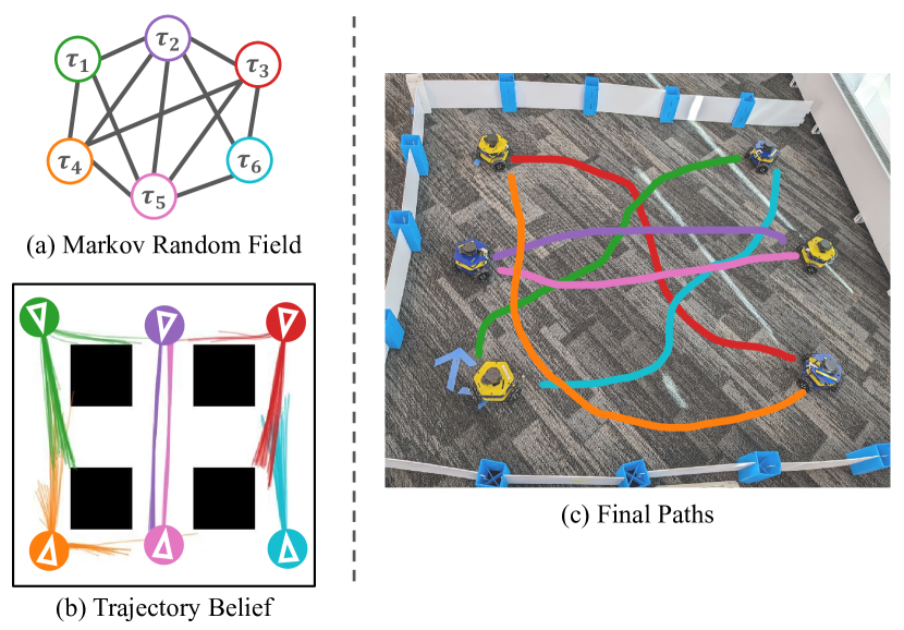
Figure 1: Stein Variational Belief Propagation (SVBP) computes marginal trajectory distributions for each robot in a multi-robot system. SVBP represents the relationships between robots as a Markov Random Field (a) and maintains multi-modal distributions over each robot trajectory (b). The final trajectory generated by SVBP for each robot is shown in (c), where the colour represents time, and the robot is shown in its final position.

In this work, we propose Stein Variational Belief Propagation (SVBP), an efficient method for performing nonparametric belief propagation [10, 11]. SVBP employs Stein Variational Gradient Descent (SVGD) [12] to update a set of particles representing the marginal posteriors, eliminating the need for sampling and fully leveraging gradient information. We formulate our SVBP algorithm by leveraging the particle message update rules from Particle Belief Propagation (PBP) [13]. The belief propagation framework enables multi-hop information to be passed through the graph while only passing messages between immediate neighbors. Our approach leverages SVGD to mitigate mode collapse and effectively represent multi-modal distributions compared to sampling-based methods. The algorithm is efficient and parallelizable since the particles are deterministically updated using gradient information.

We demonstrate our approach on two applications: a simulated multi-robot perception task, and a multi-robot Model-Predictive Control (MPC) task, both in simulation and on a real-world mobile robot swarm. The perception experiments show that SVBP can maintain multi-modal belief distributions in uncertain environments, leading to lower localization error compared to baselines. The planning experiments demonstrate that SVBP is more resilient to deadlock scenarios, and produces smoother trajectories resulting faster time-to-goal. Our robot experiments show that our SVBP controller is robust to noisy localization and dynamics and asynchronous message passing. Video results are available at the following webpage: https://progress.eecs.umich.edu/projects/stein-bp.

II Related Work

II-A Multi-robot Coordination

Decentralized multi-robot coordination algorithms are those in which each robot executes a controller to satisfy individual objectives considering local information from neighbors. This technique is highly scalable to large and dynamic swarms. Optimal Reciprocal Collision Avoidance (ORCA) [2], a variant of velocity obstacles [1], demonstrates real-time collision avoidance for thousands of agents with independent objectives but are highly prone to deadlock scenarios. We focus on decentralized Model-Predictive Control and graphical approaches in this section and refer the reader to existing surveys [14, 15] for broader coverage.

Multi-robot coordination with graphical models: Probabilistic graphical models present a natural formulation for decentralized multi-robot coordination, whereby individual robots are represented by nodes in a graph and edges connect communicating robots [5]. This formulation has been used to solve for robot localization and control with Gaussian Belief Propagation [7]. Graphical representations have also been used to learn factors for robot control via graph neural networks [6, 16]. This technique requires expert trajectory demonstrations from a centralized controller for training.

Multi-robot Model Predictive Control: Decentralized model-predictive control (DMPC) has been applied to multi-agent collision avoidance problems [17, 18, 19, 20, 21, 22]. By planning over a horizon, these techniques mitigate deadlock scenarios issues but introduce complexities due to the higher dimensionality introduced. These works consider the problem of finding a single trajectory solution. In work most similar to ours, Patwardhan et al. use Gaussian Belief Propagation for collision avoidance in multi-robot planning [7]. This method restricts the trajectory distributions to Gaussian forms, and requires all factors to be linear Gaussian. In contrast, our approach can be used with any differentiable factor and uses a more flexible nonparametric distribution.

II-B Belief propagation

A number of belief propagation algorithms have been proposed in the literature. Gaussian Belief Propagation (GaBP) is an efficient algorithm when the node distributions and their corresponding factors can be represented as Gaussian [23, 24]. This method enables efficient computation and has been shown to be effective for multi-robot collision avoidance and localization [7, 25]. However, many applications in robotics are complex and multi-modal, and cannot be fully represented by unimodal Gaussian uncertainty. Nonparametric Belief Propagation (NBP) [10, 11] represents distributions nonparametrically as mixtures of Gaussians, but involves expensive product operations between mixture distributions. Particle Belief Propagation (PBP) [13] uses importance sampling to iteratively update a set of particles representing the belief, enabling the representation of arbitrarily complex distributions. PBP relies on the definition of a sampling distribution, which later work proposed to estimate via expectation maximization [26]. However, importance sampling is prone to mode collapse, an effect which has been mitigated by using multiple sampling distributions [27]. Belief propagation has been applied to robotic perception of articulated objects, using an efficient sampling-based message product technique [28], learned unary factors [29], and end-to-end learned factors [30]. While these methods enable complex representations of belief distributions, they rely on expensive sequential sampling operations.

II-C Stein Variational Inference

SVGD has proven useful in a number of robotic applications in recent years, including control, planning, and point cloud matching [31, 32, 33, 34]. SVGD has been applied to graphical models to approximate joint distributions using kernels over local node neighborhoods [35] and conditional distributions over nodes [36]. Both these methods rely on the conditional independence structure of MRFs and as such only pass messages between immediate neighbors in the graph. In contrast, our proposed method computes the marginal beliefs over nodes using belief propagation, which involves passing messages through the whole graph.

III Background: Belief Propagation

Let $G=(V,E)$ denote a Markov Random Field (MRF) with nodes $V$ and edges $E$. Let $\mathcal{X}=\{x_{s}\mid s\in V\}$ denote the set of all hidden nodes in the graph, and $\mathcal{Z}=\{z_{s}\mid s\in V\}$ denote the observed nodes corresponding to each hidden node. The joint probability of the graph $G$ can be expressed as a product of its clique potentials:

$$p(\mathcal{X},\mathcal{Z})\propto\prod_{(s,t)\in E}\psi_{st}(x_{s},x_{t})\prod_{s\in V}\phi_{s}(x_{s},z_{s}).$$ (1)

The function $\psi_{st}$ is the pairwise potential, describing the correspondence between neighboring nodes, and $\phi_{s}$ is the unary potential, describing the correspondence of a hidden variable $x_{s}$ with the observed variable $z_{s}$. Note that in the following equations, we omit the observation, $z_{s}$, from the unary potential $\phi_{s}$ for brevity.

Belief propagation estimates the marginal posterior distribution of a hidden node $s$ using the following equation:

$$p(x_{s}\mid\mathcal{Z})\propto\phi_{s}(x_{s})\prod_{t\in\rho(s)}m_{t\to s}(x_{s})$$ (2)

where $\rho(s)$ denotes the neighbors of $s$. The message from node $t$ to node $s$, $m_{t\to s}$, is defined as:

$$m_{t\to s}(x_{s})=\int_{x_{t}}\phi_{t}(x_{t})\psi_{ts}(x_{t},x_{s})\prod_{u\in\rho(t)\setminus s}m_{u\to t}(x_{t})\;dx_{t}$$ (3)

In many cases, the integral in the above equation is intractable. Sampling-based approximations are a common way to circumvent this issue.

III-A Particle Belief Propagation

Particle Belief Propagation (PBP) defines a sampling-based algorithm for computing the messages in Equation (3) for cases where the integral is intractable due to the complexity of the state space [13]. PBP represents the belief at each node with a set of $N$ particles, $\left\{x_{s}^{(i)}\mid i\in 1\dots N\right\}$. Given samples $x_{t}^{(1)},\dots,x_{t}^{(M)}$ drawn from a candidate distribution $W_{t}$, PBP defines the approximate message:

$$\hat{m}_{t\to s}(x_{s}^{(i)})=\\ \frac{1}{M}\sum_{j=1}^{M}\frac{\phi_{t}(x_{t}^{(j)})}{W_{t}(x_{t}^{(j)})}\psi_{ts}(x_{t}^{(j)},x_{s}^{(i)})\prod_{u\in\rho(t)\setminus s}m_{u\to t}(x_{t}^{(j)}).$$ (4)

This message definition is used to draw samples from the marginal posterior, $p(x_{s}\mid\mathcal{Z})$, using importance sampling.

IV Stein Variational Belief Propagation

Our SVBP algorithm represents the marginal posterior distributions nonparametrically as a set of particles as in PBP, but eliminates the need for expensive sampling operations to approximate Equation (2). SVBP uses Stein Variational Gradient Descent (SVGD) [12] to approximate the true posterior distribution with a nonparametric candidate distribution by iteratively updating the set of particles. The update rule minimizes the Kullback–Leibler (KL) divergence between the true and candidate posteriors within a function space.

At an iteration $k$, the SVGD update is applied to each particle $x_{s}^{(i)}$:

$$x_{s}^{(i)}[k] \leftarrow x_{s}^{(i)}[k-1]+\epsilon\gamma(x_{s}^{(i)}[k-1])$$ (5)

$$\begin{split}\gamma(x_{s})&=\\ &\frac{1}{N}\sum_{j=1}^{N}\kappa(x_{s}^{(j)},x_{s})\nabla_{x_{s}^{(j)}}\log p(x_{s}^{(j)})+\nabla_{x_{s}^{(j)}}\kappa(x_{s}^{(j)},x_{s})\end{split}$$ (6)

where $\kappa(x_{s},\cdot)$ is a kernel function between particles corresponding to node $s$. Intuitively, the kernel gradient term of the above equation acts as a repulsive force between particles. In practice, this characteristic prevents mode collapse in SVGD and often requires less particles to cover the space. We define the likelihood term $p(x_{s}^{(j)})$ in Equation (6) using the marginal belief from Equation (2) to obtain the SVBP likelihood gradient:

$$\nabla_{x_{s}^{(j)}}\log p(x_{s}^{(j)})=\nabla_{x_{s}^{(j)}}\log\phi_{s}(x_{s}^{(j)})\\ +\sum_{t\in\rho(s)}\nabla_{x_{s}^{(j)}}\log m_{t\to s}(x_{s}^{(j)}),$$ (7)

where $m_{t\to s}(x_{s})$ is defined via the PBP message rule from Equation (4). A distinct set of Stein particles represents the posterior belief at each node. We note that the gradient update from Equation (7) only involves evaluating gradient information from immediate neighbors, since the messages $m_{u\to t}$ in Equation (4) are not a function of $x_{s}$. This enables efficient gradient updates since the algorithm only requires backpropagating through single-hop neighbors.

In practice, we use the current belief of the neighboring node, $p(x_{t})$, as the sampling distribution, $W_{t}$, where $p(x_{t})$ is represented by Stein particles for node $t$ with equal weights. This enables efficient computation of the messages since it eliminates the need to run expensive sampling algorithms like MCMC, as originally proposed in the PBP algorithm.

We employ a synchronous message passing scheme in which all messages are computed prior to updating each node belief. This enables efficient batch computations of factors and messages suitable for execution on a GPU. However, our algorithm can be employed with other message passing schedules.

V SVBP for Multi-Robot Perception

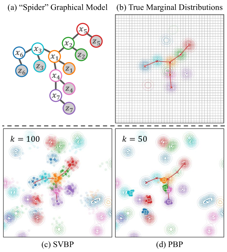
Figure 2: SVBP better represents the underlying distribution, avoiding mode collapse. (a) Graphical model of the “spider” perception problem. The $x_{i}$ nodes represent the position of each node, and the $z_{i}$ nodes represent the observation corresponding to a node. (b) The approximate true marginals for the graph in (a) and the observation shown in (c, d). Qualitative results for SVBP (c) and PBP (d) at the final iteration ($k$). The red lines represent the true position of the nodes, and the colored ‘x’ markers represent the maximum likelihood estimate for each node. Lower-weighted particles are shown with lower transparency. The distributions represent the noisy observations for each node of the corresponding color. Best viewed in color.

The first application on which we validate our algorithm is a simulated multi-robot perception experiment. The objective is to infer the belief, $p(x_{s})$, over the robot’s 2D position, denoted $x_{s}$, for each robot $s$. We consider the challenging case in which the observation for each agent is multi-modal. Specifically, the observation consists of a mixture of Gaussians which contains a component centered around the true position of the robot and randomly sampled noisy components. An example observation and the associated graphical model are shown in Figure 2. In addition to the observations, robots observe the displacement to neighboring robots, creating edges in the graph (shown in red). The resulting marginal distributions for each robot are multi-modal, as shown in Figure 2(b). We restrict the graph to a tree structure without loops for this problem. This experiment is a version of the articulated “spider” localization problem from the NBP literature [11, 28, 30].

The MRF in Figure 2 requires the definition of the potentials in Equation (1). We define the unary potential for each robot to be the mixture of Gaussians corresponding to the robot observation. The pairwise potential is defined as a function of the observed translation $L$ between neighboring robots:

$$\psi_{ts}(x_{t},x_{s})=\exp\Big{(}-\alpha\big{(}\|x_{s}-x_{t}\|-L\big{)}\Big{)}.$$ (8)

where $x_{s}$ and $x_{t}$ are the 2D positions of neighboring robots.We use $L=1$ m for all edges.

Baseline: We implement Particle Belief Propagation as a baseline approach. We employ iterative importance sampling over the particles at each node, where each particle is weighted according to Equation (2) with the message definition of Equation (4). We use the current particle set at each neighboring node as the candidate distribution for message computation, with equal weights, as in SVBP. We apply random noise at the beginning of each iteration. The same factor definitions and parameters are used for PBP and SVBP.

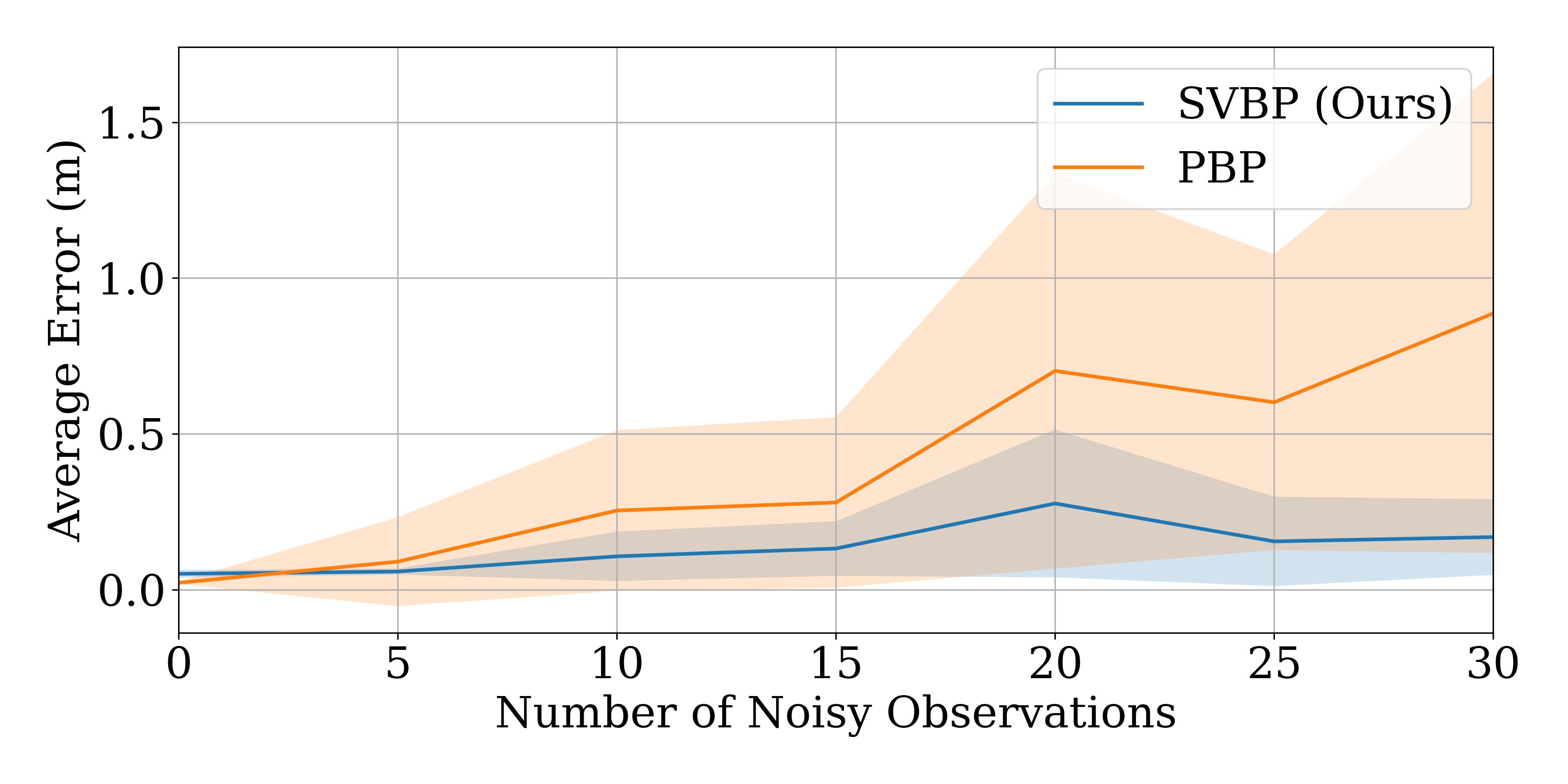
Figure 3: Average error for each node estimate for multi-robot localization. Results are shown for varying levels of noise, corresponding to the number of noisy components added to the observation.

V-A Results

To generate an estimate for each node’s position, we select the highest weighted particle according to the marginal posteriors and compute the error compared to the ground truth. The average error for each node over 10 runs for our SVBP algorithm against PBP is shown in Figure 3. The $x$-axis represents the total number of noisy Gaussian components added to the node observations. For each run, the number of noisy components are randomly assigned across nodes, making each observation a Gaussian mixture. SVBP ran for 100 optimization iterations, and PBP ran for 50 iterations. A visualization of the final belief distributions of SVBP and PBP for the highest noise observation is shown in Figure 2.

SVBP performs comparatively to PBP for low observation noise, but significantly outperforms PBP in noisy cases. We observed that PBP tends to converge quickly but was subjected to mode collapse which results in locally optimal estimates. In contrast, SVBP maintains multiple modes, making it more likely that the global solution is represented in the candidate particle set.

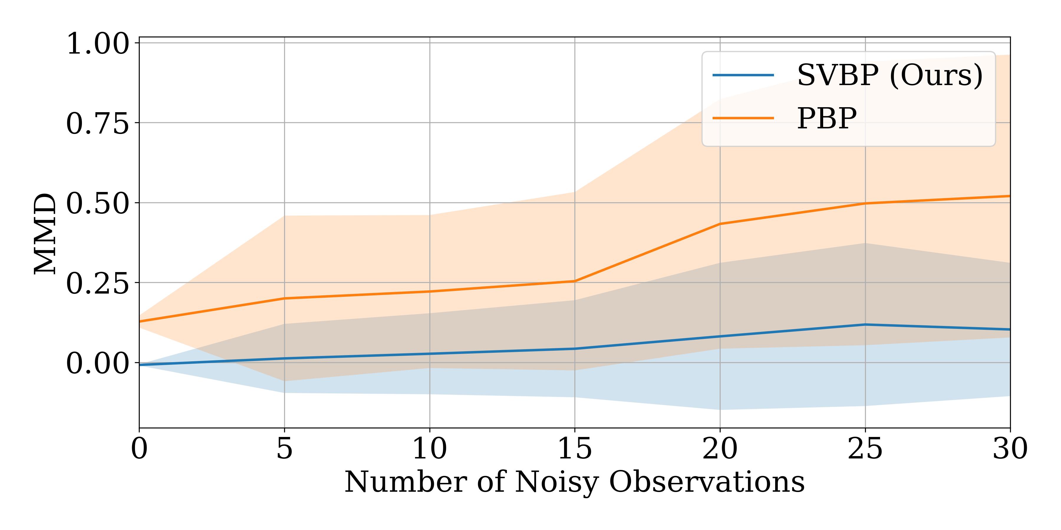
Figure 4: The average Maximum Mean Discrepency (MMD) between the samples from the true marginal distribution and the particle sets from SVBP and PBP. Both methods use 50 particles.

V-A1 Comparison to True Marginals

We hypothesize that SVBP better represents the true marginal distributions. In order to verify this hypothesis, we perform an analysis of the particle distribution of each method compared to the true marginal beliefs. To obtain the true marginal beliefs, we run a Gibbs simulation [37] to sample from the marginal using the density from Equation (2). To evaluate the integral for the message in Equation (3), we employ Monte-Carlo integration over the full region of the observation with a high number of samples (1000). The ground truth sampled marginals are imperfect due to the sampling procedure and occasionally miss modes in the true distribution, but in general provide a reasonable baseline approximation. The visualization of the true marginal is shown in Figure 2(b).

We compute the kernelized Maximum Mean Discrepancy (MMD) [38] between the sampled particle set and the belief particles for SVBP and PBP. The kernel bandwidth is chosen using the median heuristic over the ground truth sample set [39]. Results are shown in Figure 4. SVBP obtains a lower MMD than PBP consistently across noisy environments. We observe that some particles in SVBP get caught in local minima in very noisy cases in areas where the unary potential is high, as in Figure 2(c). These particles are easily detected as they have very low overall weights and could be reset in practice. We therefore do not include any particles with weights less than 1% of the highest weight in the MMD computation.

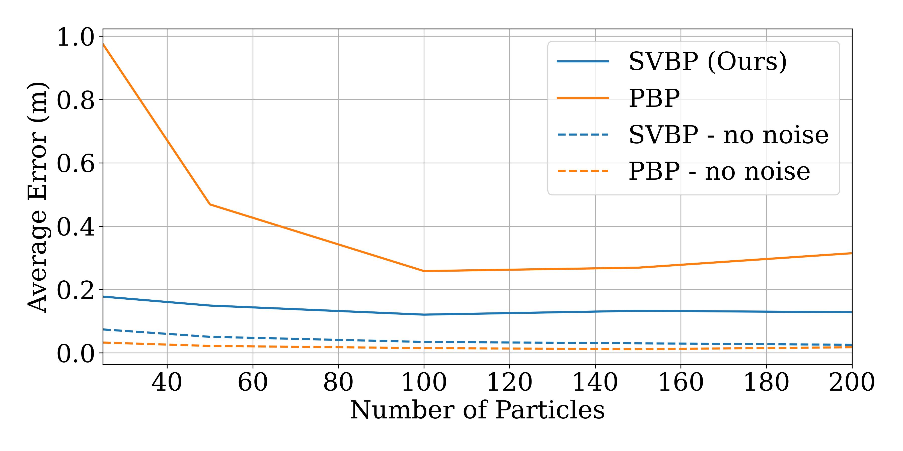
Figure 5: Average error for each node estimate for different numbers of particles. The solid lines correspond to experiments runs with noise added to the observation. The dashed lines correspond to experiments with no noise added to the observation.

V-A2 Analysis of Number of Particles

We claim that SVBP can represent the marginal beliefs with fewer particles due to SVGD’s ability to maintain modes of the distribution. We execute both SVBP and PBP with different particle set sizes and measure the average error across each node for the final estimate. The results are shown in Figure 5. For noisy environments, PBP benefits significantly when the size of the particle set is increased from 25 to 100, whereas SVBP finds a good estimate even when the number of particles is as low as 25. For environments with no noise, PBP has a slight advantage over SVBP since the particles are allowed to collapse to the true estimate, whereas SVBP particles might not converge to the true value due to the repulsive force. This could be mitigated by performing gradient descent without the Stein update after convergence to improve the final estimate.

VI SVBP for Multi-Robot Planning

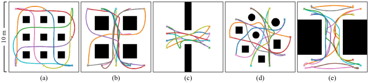
Figure 6: Testing environments for the multi-robot control experiments with randomly selected trajectories from SVBP. The goal positions for each robot are marked with an ‘x’. Each environment is 10 meters by 10 meters.

Our second application involves decentralized Model Predictive Control (MPC) of a multi-robot system. Each robot must avoid obstacles and the other robots in its trajectory to the goal. We run experiments both in a 2D planar navigation simulation and on a decentralized real robot system with realistic sensor and action noise.

VI-A Problem Formulation

We consider the problem of finding a collision-free trajectory for each robot $s$, $\tau_{s}=\{u_{s,k}\mid 1\leq k\leq T\}$, where $u_{s,k}$ are control commands for time $k$ over a fixed horizon $T$. We take a planning as inference approach [3, 4] in which the nodes in the graph represent the trajectory distribution, $p(\tau_{s})$ for each robot, and the edges in the graph represent robots in communication, as in Figure 1. We assume known dynamics $x_{s,k+1}=f_{s}(x_{s,k},u_{s,k})$, where $x_{s,k}$ is the state of robot $s$ at time $k$, and a known initial state $x_{s,0}$. At each timestep, we execute the first action in the trajectory and rerun the optimization, as in model predictive control (MPC). This approach is akin to a multi-robot version of Stein MPC [31].

For this experiment, we assume the graph is fully-connected. We employ a loopy version of belief propagation, in which the messages are initialized and iteratively updated. This approach does not provide exact marginals but has proven to be effective in practice [40].

Potential functions: The unary potential for each robot trajectory is defined with respect to the running cost $c(x_{s,k},u_{s,k})$ and terminal cost $C(x_{s,T})$ for a trajectory:

$$\phi_{s}(\tau_{s},x_{s,0})=\exp-\left(C(x_{s,T})+\sum_{k=1}^{T-1}\gamma_{k}\,c_{s}(x_{s,k},u_{s,k})\right)$$ (9)

where $T$ is the time horizon and $\gamma_{k}$ are constants. The running cost consists of a quadratic cost and an obstacle avoidance cost based on the signed-distance function for the obstacles. Intermediate state values $x_{s,k}$ needed to compute the costs are obtained by simulated rollouts using the dynamics, $f_{s}(x_{s,k},u_{s,k})$.

The pairwise potential between communicating robots employs the following collision avoidance factor over the trajectory:

$$\begin{split}\log&\;\psi_{ts}(\tau_{t},\tau_{s})=\\ &-\sum_{k=0}^{T}\begin{cases}\alpha_{k}\left(1-\left(\frac{d(x_{s,k},x_{t,k})}{r}\right)^{\beta}\right)&d(x_{s,k},x_{t,k})\leq r\\ 0&d(x_{s,k},x_{t,k})>r\\ \end{cases}\end{split}$$ (10)

where $d(x_{s,k},x_{t,k})$ is the distance between the robot positions at timestep $k$, $r$ is the desired collision radius, and $\alpha_{k}$ and $0<\beta\leq 1$ are constants. In our experiments, we use $r=0.5$ and $\beta=0.3$. We set $\alpha_{k}$ to decrease linearly over the horizon.

Given differentiable dynamics, the above potential definitions allow the gradients from Equation (7) to be computed with respect to the trajectories $\tau_{s}$. We use a Gaussian kernel which employs a distance function computed as the sum of the Euclidean distance between states in two trajectories at corresponding times. Equation (6) is applied iteratively to obtain a set of trajectories comprising the belief for each robot, $\{\tau_{s}^{(i)}\mid 1\leq i\leq N\}$.

VI-B Baselines

Two baselines are employed for this scenario: the well-established Optimal Reciprocal Collision Avoidance (ORCA) algorithm [2], and Gaussian Belief Propagation (GaBP), as in [7]. ORCA assumes that neighboring agent’s velocity are known and calculates optimal reciprocally collision-avoiding velocities that are closest to the original preferred velocity. The scenario was implemented using the RVO2 library [41]. We assume full connectivity.

For GaBP, potentials are expressed as a linearized Gaussian factor [24] with a bias term that encodes the expected joint Gaussian to be observed. In contrast to the formulation by Patwardhan et al. [7], we represent the trajectory consisting of 2D acceleration commands for one robot as a single node, rather than inferring the state at individual timesteps. We use similar potential functions to our SVBP implementation for fair comparison. The factors in GaBP are restricted to the form:

$$E_{s}(\tau_{s})=\frac{1}{2}(h_{s}(\tau_{s})-b_{s})^{\top}\Sigma_{s}^{-1}(h_{s}(\tau_{s})-b_{s})$$ (11)

where $h_{s}(\tau_{s})$ is an “observation function” over the trajectory $\tau_{s}$, $b_{s}$ is a bias term, and $\Sigma_{s}$ is the covariance [24].

In order to use our non-linear, non-Gaussian costs, we set $h_{s}(\tau_{s})$ to be the cost for each of our factors, with $b_{s}=0$. Since our costs are non-linear, $h_{s}(\tau_{s})$ must be linearized about an estimate via a first-order Taylor series expansion. As in SVBP, the linearization requires backpropagation through the dynamics $f_{s}(x_{s,k},u_{s,k})$. Since the quadratic cost is already linear, we use $h_{s}(\tau_{s})=\begin{bmatrix}X_{s}&\tau_{s}\end{bmatrix}$, where $X_{s}$ is the state vector from simulated trajectory rollouts using the dynamics model. Our GaBP implementation is able to infer optimal trajectories without the need of a trajectory planner by making use of the dynamics function, in contrast to the formulation by Patwardhan et al. [7].

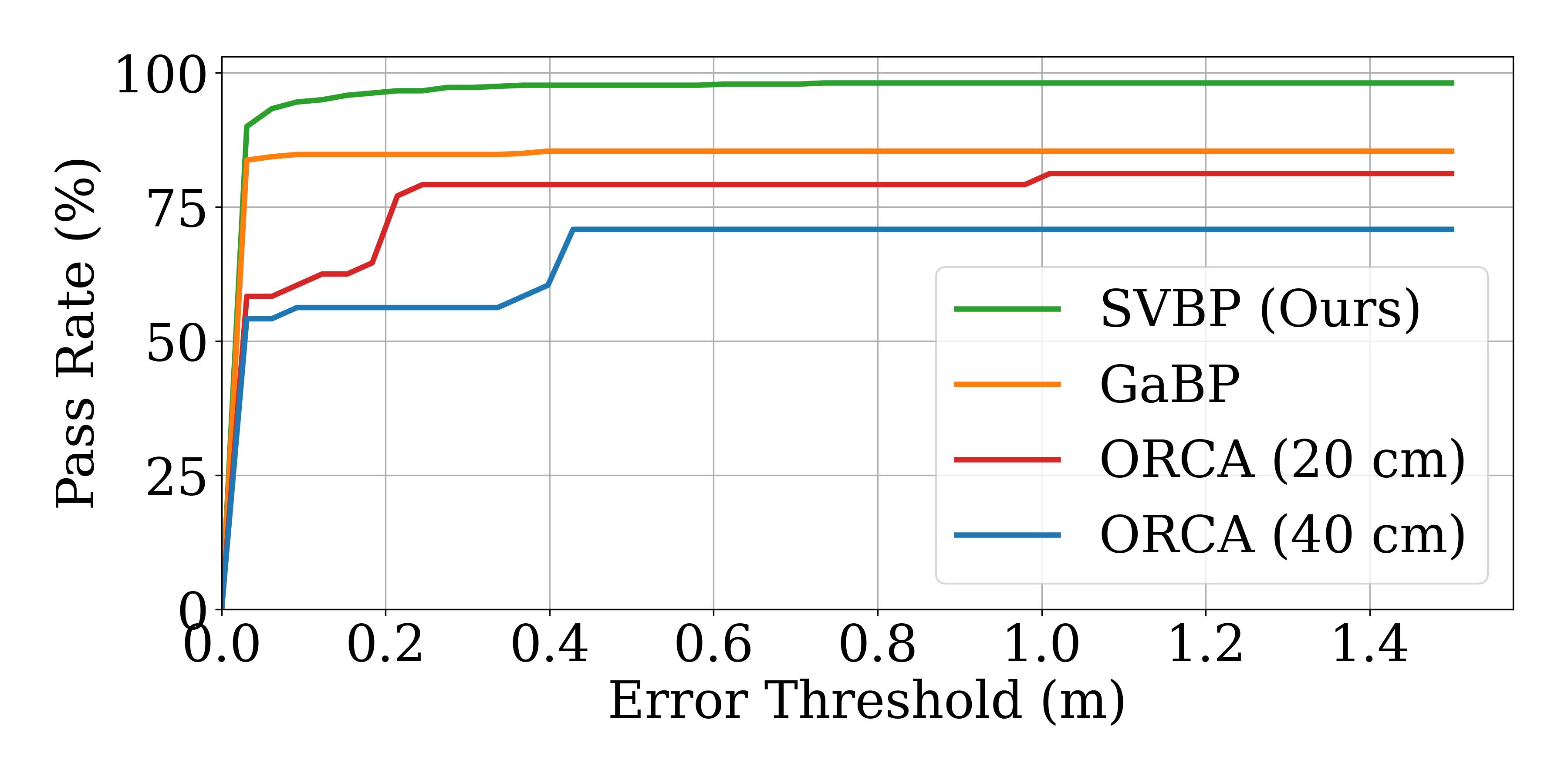
Figure 7: Pass rate for each method considered for the multi-robot control example. The pass rate represents the percentage of trajectories which finished within a given error threshold.

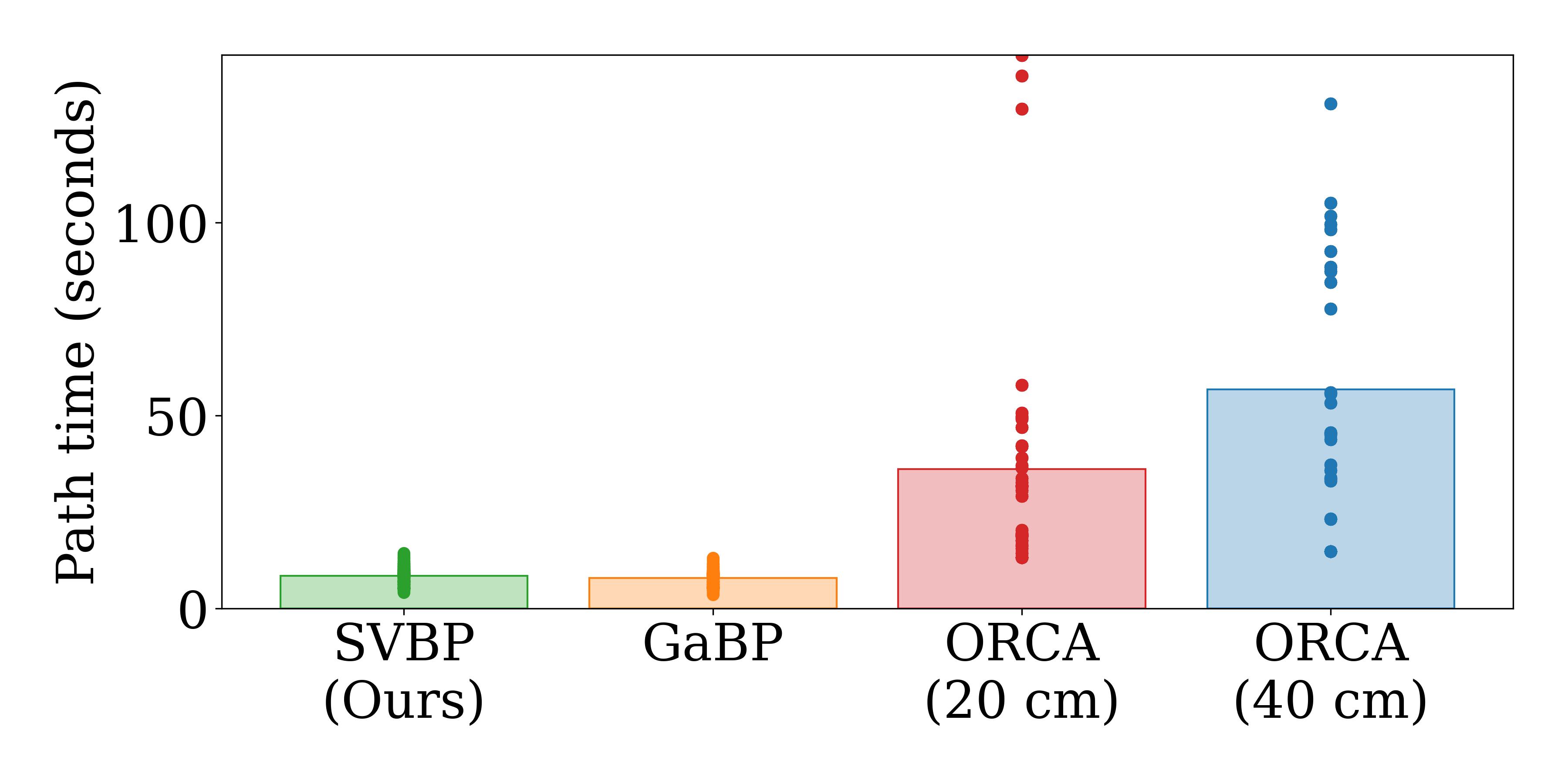
Figure 8: Path time for each method considered for the multi-robot control example. Only successful results are included for path time analysis. A trajectory is successful if it reaches the goal within 30 cm without collisions.

VI-C Simulated Robot Experiments

We perform the simulated experiments in acceleration space, where the state $x_{s,k}$ consists of 2D position and velocity, and the control commands $u_{s,k}$ are 2D accelerations. We use a time horizon of 20 discrete steps of 0.1 seconds each, making $\tau_{s}$ 40 dimensional for each robot. The first control command from the lowest cost trajectory is executed at each timestep. The optimization is then rerun in MPC-style.

Results: We present the pass rate for ORCA, GaBP, and SVBP in Figure 7. The pass rate represents the percentage of trajectories ($y$-axis) which reached the goal within a given error threshold ($x$-axis) across all robots for each run. Any robots that collided with another robot are not counted as passed for any threshold. Since ORCA is sensitive to the robot radius parameter, we show results for both a radius of 20 cm and 40 cm. We perform 10 runs on each of the environments in Figure 6. The total path time for each method is shown in Figure 8. Path time is only computed for trajectories which terminated within 30 cm of the goal without collisions. While all methods result in similar path lengths, the robots move much more conservatively in the ORCA baseline, which results in higher path times.

We observe that the failure modes in SVBP can occur due to local minima, for example around large obstacles such as in the environments in Figure 6(c, e). GaBP is especially susceptible to getting caught in local minima in the presence of challenging obstacles. A subset of robots fail to reach their goals for every run in one environment, as illustrated in Figure 9(b). OCRA is particularly prone to deadlock scenarios when it must obey a collision tolerance (i.e. 40 cm collision radius case), failing for all runs in the environment shown in Figure 9(a).

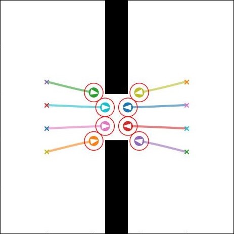
(a) ORCA (40 cm)

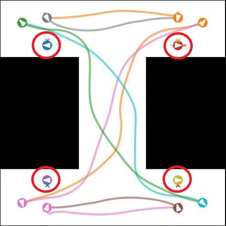
(b) Gaussian Belief Propagation

Figure 9: Failure modes for the baselines considered for the planar navigation experiment. (a) ORCA is prone to deadlock, especially in the presence of obstacles. All run for this environment fail with a 40 cm radius (shown with red circles). (b) Gaussian Belief Propagation is prone to falling into local minima, especially around large objects. The four robots circled in red cannot get around the obstacles.

VII Real Robot Experiments

We run our controller on a real multi-robot system comprised of omni-directional robot platforms. We perform a collision avoidance experiment with three robots where the robots must cross paths to reach their goal locations. The goal of this experiment is to determine the performance of our controller under 1) noisy perception and dynamics, 2) limited computing resources, 3) realistic asynchronous message passing schedules. The robots are equipped with a single-board computer with limited processing power (a Raspberry Pi) and pass messages through a custom websocket interface over a WiFi connection. We employ particle-based Monte-Carlo Localization using a 2D Lidar for state estimation [42]. The swarm is assumed to be fully-connected.

Decentralized Message Passing: Each robot independently maintains a representation of the graph and updates messages within their local graph based on neighbor belief. At the beginning of each optimization iteration, the robots request the current trajectory distribution from their neighbors which is used to update the local messages in each robot’s representation of the graph. The robots pass messages using a custom API which passes messages through websockets, inspired by rosbridge [43], which allows them to synchronously query data from robots on a shared network.

Baseline: ORCA is implemented on the robots as a baseline. The algorithm is run in a centralized manner on a single robot which broadcasts velocity commands to the whole fleet. ORCA outputs a velocity command for each robot rather than a trajectory, therefore we do not use an external trajectory tracker and execute the velocity command directly.

Implementation Details: We perform the simulated experiments in velocity space, where the state $x_{s,k}$ consists of 2D position and the control commands $u_{s,k}$ are 2D velocities. We plan over 10 discrete timesteps, with a 0.25 second timestep. We first perform 15 initialization iterations over random trajectory particles before beginning execution. The lowest cost trajectory is chosen and executed by a closed-loop velocity controller. The optimization is repeated until the goal is reached in MPC-style, initializing using particles from the previous timestep.

VII-A Results

We perform 5 runs on a scene with and without collisions (10 runs total) for SVBP and ORCA. The time-to-goal results are shown in Figure 11. On the scene with no obstacles, SVBP reaches the goal in all runs with no collisions except for in one run, in which one robot has a localization failure resulting in a collision. We find that ORCA deadlocks at the start of the trajectory for all runs. To obtain meaningful comparisons, we manually perturb the robots from their start positions until they escape the deadlock. ORCA’s built-in random perturb for deadlock prevention is not sufficient to overcome deadlock in practice as the physical robots require higher commanded velocities to overcome static forces, but ORCA tends to select low speeds unless large clearances are available. Modification of the perturbation functionality for this application could mitigate this issue. After the deadlock is resolved, ORCA and SVBP achieve similar time-to-goal in scenarios without obstacles.

For the case with obstacles, ORCA deadlocks at the beginning of the run two cases. However, the algorithm gets stuck in deadlock for 2 of 5 runs near the obstacle, and the deadlock results in a collision in one of the cases (robots #2 and #3 do not reach the goal in 2 cases in Figure 11, right). We only apply manual perturbation for deadlocks for ORCA at the beginning of the run. SVBP reaches the goals in all the cases, and in generally smoother paths. One robot #2 is prone to stopping when the robots cross paths, but eventually reaches the goal. A visualization of an execution of SVBP with obstacles is shown in Figure 10.

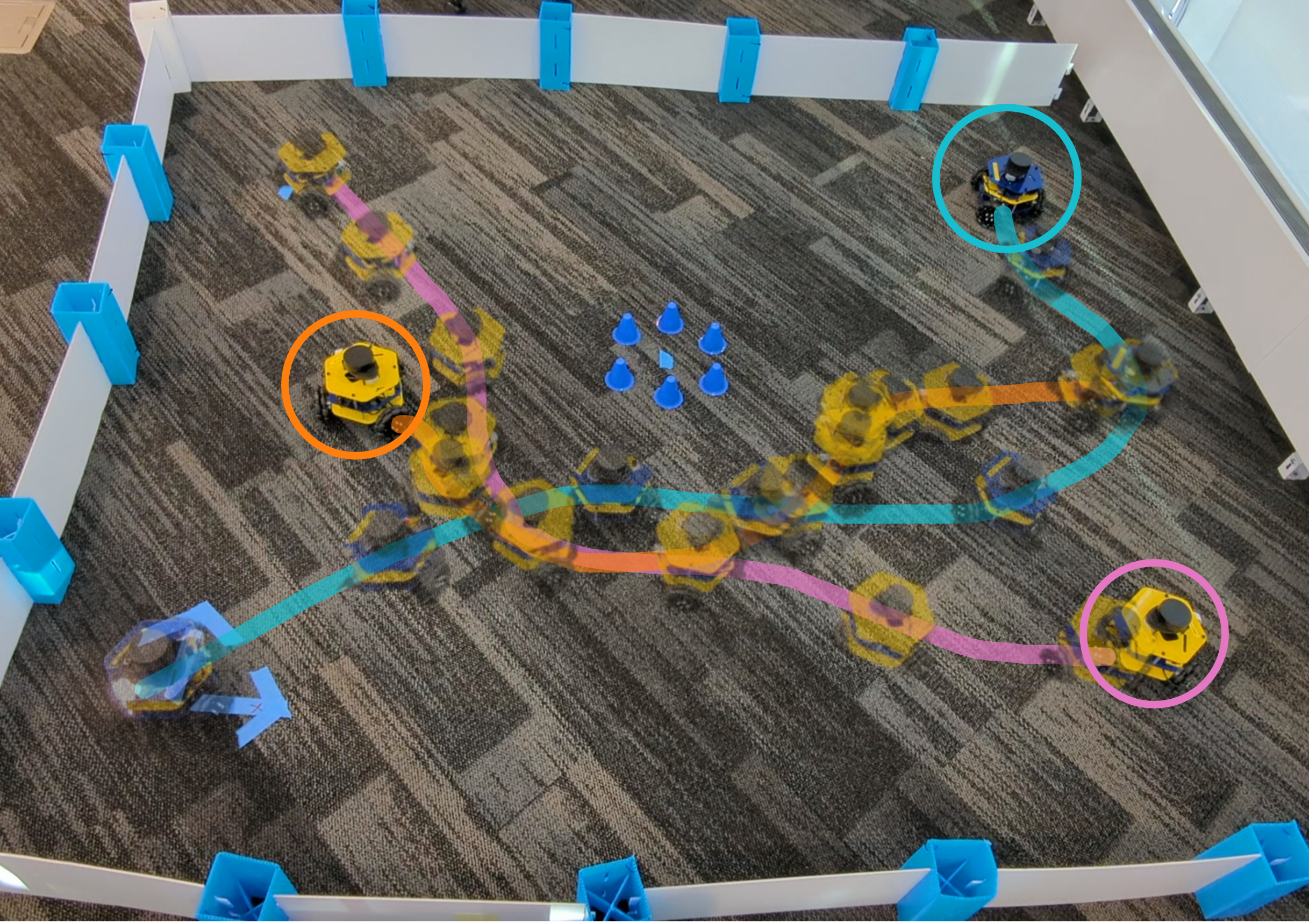
Figure 10: An example of a trajectory for the SVBP algorithm on a real robot. The circles highlight the final goal position for each robot.

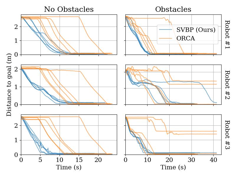
Figure 11: Distance to the goal over time for each robot for runs with no obstacles (left) and with obstacles (right).

VIII Discussion & Conclusion

We present Stein Variational Belief Propagation (SVBP), an algorithm for inferring nonparametric marginal beliefs in graphs using Stein Variational Gradient Descent. We demonstrate the applicability of our algorithm on two applications: simulated multi-robot perception, and multi-robot planning both in simulation and on real robots. Through simulated perception experiments, we show that SVBP approximates the true marginal distributions better and is more particle efficient than sampling-based baselines. The planning experiments show that the algorithm is more effective at escaping local-minima and deadlock scenarios than baselines. The real-world planning experiments show that the method is robust to realistic noise.

A limitation of the proposed algorithm is that the computation time scales with the number of neighbors. We limited the robot experiments to three robots in order to achieve fast enough execution to run MPC on the single-board computers on the robots. Future work will involve improving the implementation efficiency in order to increase the size of the swarm. Another limitation for decentralized control is the need to time-synchronize incoming neighbor messages from other robots. We observe that the robots are prone to starting and stopping behavior when near other robots which we posit occurs due to lack of time synchronization. This could be mitigated by accounting for the time delays between messages. Further study is needed on the impact of message delays and packet loss [16].

Our robot experiments show that our method is robust to realistic perception and action uncertainty, despite the fact that we do not explicitly model this uncertainty. Integrating perception and action noise models into the model in order to deal with more challenging scenarios is an interesting avenue of investigation. We hypothesize that this could also help scale the algorithm to cases with nonlinear dynamics.

IX Acknowledgements

This work was supported in part by Ford Motor Company, J.P. Morgan AI Research, Amazon, the Alfred P. Sloan Foundation, and an NSERC doctoral fellowship.

References

- [1] P. Fiorini and Z. Shiller, “Motion planning in dynamic environments using velocity obstacles,” The international journal of robotics research, vol. 17, no. 7, pp. 760–772, 1998.
- [2] J. Van Den Berg, S. J. Guy, M. Lin, and D. Manocha, “Reciprocal n-body collision avoidance,” in Robotics Research: The 14th International Symposium (ISRR). Springer, 2011, pp. 3–19.
- [3] H. Attias, “Planning by probabilistic inference,” in International Workshop on Artificial Intelligence and Statistics, ser. Proceedings of Machine Learning Research, vol. R4. PMLR, 2003, pp. 9–16.
- [4] M. Toussaint, “Robot trajectory optimization using approximate inference,” in International Conference on Machine Learning (ICML), 2009, pp. 1049–1056.
- [5] J. N. Schwertfeger and O. C. Jenkins, “Multi-robot belief propagation for distributed robot allocation,” in 2007 IEEE 6th international conference on development and learning. IEEE, 2007, pp. 193–198.
- [6] E. Tolstaya, F. Gama, J. Paulos, G. Pappas, V. Kumar, and A. Ribeiro, “Learning decentralized controllers for robot swarms with graph neural networks,” in Conference on robot learning. PMLR, 2020, pp. 671–682.
- [7] A. Patwardhan, R. Murai, and A. J. Davison, “Distributing collaborative multi-robot planning with Gaussian belief propagation,” Robotics and Automation Letters, vol. 8, no. 2, pp. 552–559, 2022.
- [8] J. Butterfield, O. C. Jenkins, D. M. Sobel, and J. Schwertfeger, “Modeling aspects of theory of mind with markov random fields,” International Journal of Social Robotics, vol. 1, pp. 41–51, 2009.
- [9] M. J. Wainwright, M. I. Jordan et al., “Graphical models, exponential families, and variational inference,” Foundations and Trends in Machine Learning, vol. 1, no. 1–2, pp. 1–305, 2008.
- [10] E. B. Sudderth, A. T. Ihler, M. Isard, W. T. Freeman, and A. S. Willsky, “Nonparametric belief propagation,” Communications of the ACM, vol. 53, no. 10, pp. 95–103, 2010.
- [11] M. Isard, “PAMPAS: Real-valued graphical models for computer vision,” in Computer Vision and Pattern Recognition (CVPR), vol. 1, 2003.
- [12] Q. Liu and D. Wang, “Stein variational gradient descent: A general purpose Bayesian inference algorithm,” Advances in Neural Information Processing Systems, vol. 29, 2016.
- [13] A. Ihler and D. McAllester, “Particle belief propagation,” in Artificial Intelligence and Statistics, 2009, pp. 256–263.
- [14] B. P. Gerkey and M. J. Matarić, “A formal analysis and taxonomy of task allocation in multi-robot systems,” The International journal of robotics research, vol. 23, no. 9, pp. 939–954, 2004.
- [15] F. Rossi, S. Bandyopadhyay, M. T. Wolf, and M. Pavone, “Multi-agent algorithms for collective behavior: A structural and application-focused atlas,” arXiv preprint arXiv:2103.11067, 2021.
- [16] E. Tolstaya, L. Butler, D. Mox, J. Paulos, V. Kumar, and A. Ribeiro, “Learning connectivity for data distribution in robot teams,” in International Conference on Intelligent Robots and Systems (IROS). IEEE, 2021, pp. 413–420.
- [17] D. Morgan, S.-J. Chung, and F. Y. Hadaegh, “Model predictive control of swarms of spacecraft using sequential convex programming,” Journal of Guidance, Control, and Dynamics, vol. 37, no. 6, pp. 1725–1740, 2014.
- [18] H. Y. Ong and J. C. Gerdes, “Cooperative collision avoidance via proximal message passing,” in 2015 American Control Conference (ACC), 2015, pp. 4124–4130.
- [19] R. Van Parys and G. Pipeleers, “Distributed model predictive formation control with inter-vehicle collision avoidance,” in 2017 11th Asian Control Conference (ASCC), 2017, pp. 2399–2404.
- [20] L. Dai, Q. Cao, Y. Xia, and Y. Gao, “Distributed MPC for formation of multi-agent systems with collision avoidance and obstacle avoidance,” Journal of the Franklin Institute, vol. 354, no. 4, pp. 2068–2085, 2017.
- [21] C. E. Luis, M. Vukosavljev, and A. P. Schoellig, “Online trajectory generation with distributed model predictive control for multi-robot motion planning,” IEEE Robotics and Automation Letters, vol. 5, no. 2, pp. 604–611, 2020.
- [22] Z. Cheng, J. Ma, X. Zhang, C. W. de Silva, and T. H. Lee, “ADMM-based parallel optimization for multi-agent collision-free model predictive control,” arXiv preprint arXiv:2101.09894, 2021.
- [23] Y. Weiss and W. Freeman, “Correctness of belief propagation in gaussian graphical models of arbitrary topology,” Advances in neural information processing systems, vol. 12, 1999.
- [24] A. J. Davison and J. Ortiz, “FutureMapping 2: Gaussian belief propagation for spatial AI,” arXiv preprint arXiv:1910.14139, 2019.
- [25] R. Murai, J. Ortiz, S. Saeedi, P. H. Kelly, and A. J. Davison, “A robot web for distributed many-device localisation,” arXiv preprint arXiv:2202.03314, 2022.
- [26] T. Lienart, Y. W. Teh, and A. Doucet, “Expectation particle belief propagation,” in Advances in Neural Information Processing Systems, 2015, pp. 3609–3617.
- [27] J. Pacheco, S. Zuffi, M. Black, and E. Sudderth, “Preserving modes and messages via diverse particle selection,” in International Conference on Machine Learning (ICML), vol. 32, no. 2, 2014, pp. 1152–1160.
- [28] K. Desingh, S. Lu, A. Opipari, and O. C. Jenkins, “Efficient nonparametric belief propagation for pose estimation and manipulation of articulated objects,” Science Robotics, vol. 4, no. 30, 2019.
- [29] J. Pavlasek, S. Lewis, K. Desingh, and O. C. Jenkins, “Parts-based articulated object localization in clutter using belief propagation,” in International Conference on Intelligent Robots and Systems (IROS). IEEE, 2020.
- [30] A. Opipari, J. Pavlasek, C. Chen, S. Wang, K. Desingh, and O. C. Jenkins, “DNBP: Differentiable nonparametric belief propagation,” ACM Journal of Data Science, vol. 1, no. 1, 2023.
- [31] A. Lambert, A. Fishman, D. Fox, B. Boots, and F. Ramos, “Stein variational model predictive control,” in Conference on Robot Learning (CoRL), 2020.
- [32] L. Barcelos, A. Lambert, R. Oliveira, P. Borges, B. Boots, and F. Ramos, “Dual online Stein variational inference for control and dynamics,” in Robotics: Science and Systems (RSS), 2021.
- [33] F. A. Maken, F. Ramos, and L. Ott, “Stein ICP for uncertainty estimation in point cloud matching,” Robotics and Automation Letters, vol. 7, no. 2, pp. 1063–1070, 2022.
- [34] A. Lambert, B. Hou, R. Scalise, S. S. Srinivasa, and B. Boots, “Stein variational probabilistic roadmaps,” in International Conference on Robotics and Automation (ICRA). IEEE, 2022, pp. 11 094–11 101.
- [35] D. Wang, Z. Zeng, and Q. Liu, “Stein variational message passing for continuous graphical models,” in International Conference on Machine Learning. PMLR, 2018, pp. 5219–5227.
- [36] J. Zhuo, C. Liu, J. Shi, J. Zhu, N. Chen, and B. Zhang, “Message passing Stein variational gradient descent,” in International Conference on Machine Learning. PMLR, 2018, pp. 6018–6027.
- [37] G. Casella and E. I. George, “Explaining the gibbs sampler,” The American Statistician, vol. 46, no. 3, pp. 167–174, 1992.
- [38] A. Gretton, K. M. Borgwardt, M. J. Rasch, B. Schölkopf, and A. Smola, “A kernel two-sample test,” The Journal of Machine Learning Research, vol. 13, no. 1, pp. 723–773, 2012.
- [39] D. Garreau, W. Jitkrittum, and M. Kanagawa, “Large sample analysis of the median heuristic,” arXiv preprint arXiv:1707.07269, 2017.
- [40] K. P. Murphy, Y. Weiss, and M. I. Jordan, “Loopy belief propagation for approximate inference: An empirical study,” in Conference on Uncertainty in Artificial Intelligence (UAI), ser. UAI’99. Morgan Kaufmann Publishers Inc., 1999, p. 467–475.
- [41] J. Van Den Berg, S. J. Guy, J. Snape, M. Lin, and D. Manocha. (2016) RVO2 library: Reciprocal collision avoidance for real-time multi-agent simulation. [Online]. Available: https://gamma.cs.unc.edu/ORCA/
- [42] S. Thrun, W. Burgard, and D. Fox, Probabilistic Robotics. MIT Press, 2005.
- [43] C. Crick, G. Jay, S. Osentoski, B. Pitzer, and O. C. Jenkins, “rosbridge: ROS for non-ROS users,” in Robotics Research: The 15th International Symposium ISRR. Springer, 2017, pp. 493–504.