Diffusive evaporation dynamics in polymer solutions is ubiquitous

Abstract

Recent theory and experiments have shown how the buildup of a high-concentration polymer layer at a one-dimensional solvent-air interface can lead to an evaporation rate that scales with time as $t^{-1/2}$ and that is insensitive to the ambient humidity. Using phase field modelling we show that this scaling law constitutes a naturally emerging robust regime, Diffusion-Limited Evaporation (DLE). This regime dominates the dynamical state diagram of the system, which also contains regions of constant and arrested evaporation, confirming and extending understanding of recent experimental observations and theoretical predictions. We provide a theoretical argument to show that the scaling observed in the DLE regime occurs for a wide range of parameters, and our simulations predict that it can occur in two-dimensional geometries as well. Finally, we discuss possible extensions to more complex systems.

Evaporating aqueous polymer solutions are found everywhere: from industrial coatings to foods and even respiratory aerosols. Surprisingly, recent experiments suggest that such solutions evaporate in a way that is fundamentally different from pure water. The buildup of a concentrated polymer layer at the water-air interface hinders evaporation and slows down the process. We use theory and computer simulations to investigate the ubiquitous nature of this phenomenon in a one-dimensional model. We then show how our model can be generalised to more realistic and complex systems. Our results provide insights for understanding many practical applications, from the survival of viruses in respiratory droplets to how oil paintings dry slowly over time.

Solvent evaporation from concentrated solutions or suspensions is an omnipresent phenomenon. The apparent simplicity of this process is deceptive: it is in fact ridden with complications due to the interaction between multiple components and the environment, leading to complex and fascinating dynamics. Such dynamics can in turn fundamentally alter the evaporative behaviour. Its understanding is therefore important for designing or controlling any process that involves drying. For instance, evaporative dynamics controls the application of paints and inks, where the formation of a defect-free skin upon drying is desired [1]. It is also important in food preservation, where moisture content reduction increases shelf-life, but may also adversely affect flavour or texture [2]. Due to such practical applications and fundamental interest in the dynamics of multi-component complex systems, the physics of evaporating polymer solutions and colloidal suspensions has inspired numerous investigations [3, 4, 5, 6, 7].

A number of these pertain to quasi-one-dimensional evaporation from the open end of a long capillary. In this geometry, the phase behaviour of aqueous lipid solutions can respond to varying ambient water activity $a_{e}$ (equivalently, relative humidity) in such a way as to render the evaporation rate practically independent of $a_{e}$ [5]. It is suggested that in this regime, the mass flux is diffusion-controlled, $J_{\text{evap}}\sim t^{-1/2}$. A similar regime was predicted theoretically by Salmon et al. [6]. They argue that the evaporation-induced advective flux causes the growth of a concentrated ‘polarization layer’ at the interface, leading to mass loss increasing with the square root of time, hereafter referred to as Diffusion-Limited Evaporation (DLE). However, the stability range of this DLE regime in parameter space was not explored because current calculations assume diffusional dynamics.

We have recently tested the predictions of Salmon et al., and observed a regime of $a_{e}$-independent evaporation in which the rate decreases as $t^{-1/2}$ [8]. We also found a transition from constant evaporation rate at early times to this $t^{-1/2}$ regime, consistent with the building up of a polymeric ‘polarisation layer’. The inclusion of elastic effects from the formation of a very thin ‘gelled skin’ right at the air-solution interface [9, 10] improves the agreement between theory and experiments.

On general grounds, we expect that $J_{\text{evap}}\sim t^{-1/2}$ should only be one of at least three dynamical regimes of mass loss in an evaporating polymer solution. At very low polymer concentration, we should approach pure solvent evaporation, where the mass loss $m(t)\sim t$, giving a constant evaporation rate. In the absence of any evaporative driving force, for instance when the air is saturated with solvent, we expect $m(t)\sim t^{0}$. So, we expect that DLE, where $J_{\text{evap}}\sim t^{-1/2}$ or $m\sim t^{1/2}$, represents an intermediate regime. Surprisingly, however, this is the only behaviour observed experimentally to date at long times [5, 11, 8]. Why this is so is currently a puzzle.

We set up and investigate a continuum phase-field model for the one-dimensional hindered evaporation of a polymer solution. We indeed find three main evaporative regimes that transition into one another, with predictions for the diffusive regime that agree with other studies to date. Importantly, the DLE regime dominates the predicted state diagram of the system. We characterise the generic nature of this regime and propose an argument to explain why it is so pervasive. The physical picture that emerges is a simple one. A polymer layer grows from the interface into the bulk solution. When this layer becomes concentrated enough to act as a ‘porous plug’, Darcy solvent flow through this layer is the rate limiting step, so that the evaporative dynamics becomes diffusive. Finally, we show how the model can be extended to higher dimensions, or to study more complex systems such as aerosol droplets, important in respiratory virus transmission, or multilayered paints and coatings.

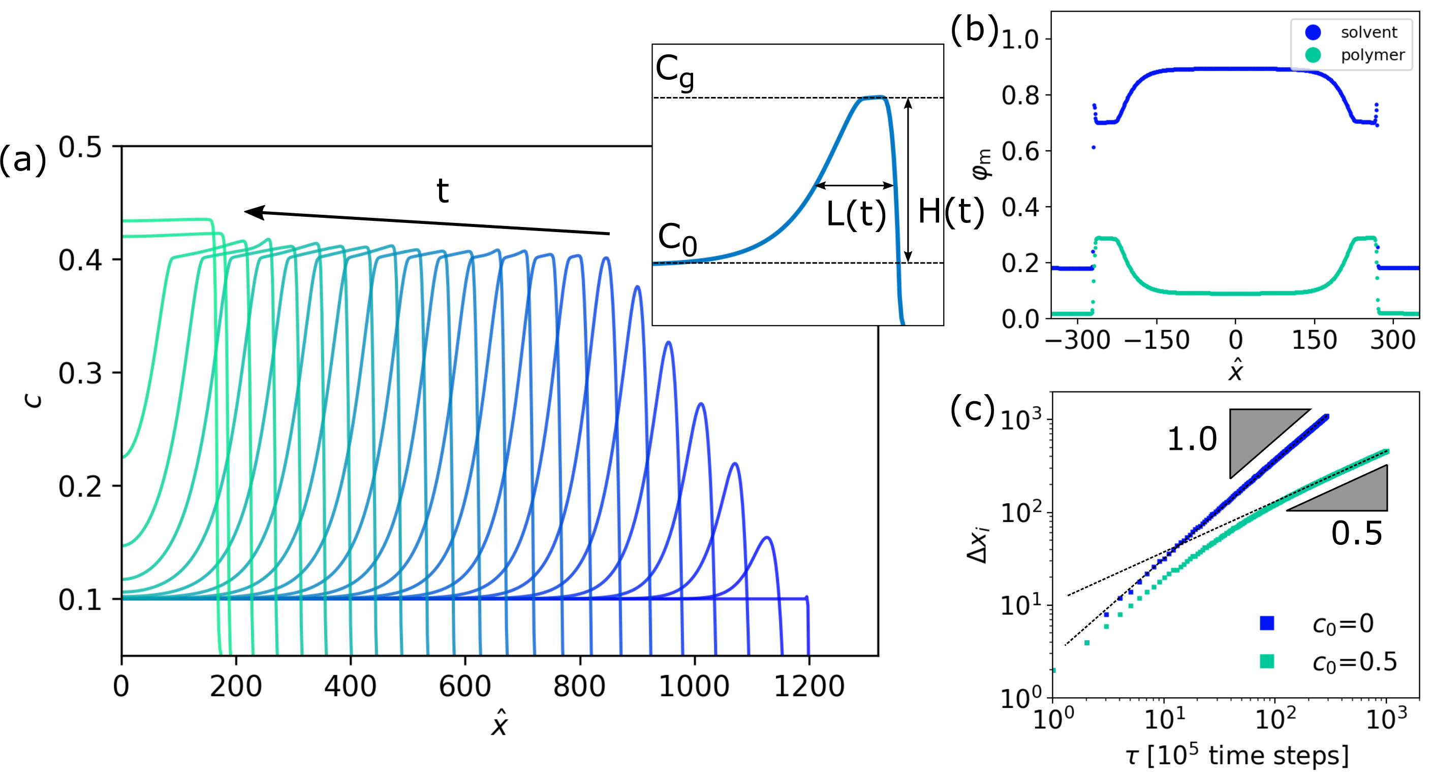
Figure 1: Dynamic evolution of a unidirectional drying polymer-solvent system in 1D. (a) Time evolution of polymer concentration profiles $c$ in a 1D polymer-solvent slab during evaporation. The arrow indicates the direction of time. Inset: schematic of the initial concentration $c_{0}$, gelation concentration $c_{g}$, width of the polymer layer $L(t)$ (taken as the Full Width Half Maximum) and the peak height of the polymer layer $H(t)$. (b) Normalized phase field of the polymer ($\varphi_{m}=\frac{c}{\phi_{1}+c}$) and the solvent ($\varphi_{m}=\frac{\phi}{\phi_{1}+c}$) at time $t=1800$. (c) Evolution of the interface $\Delta x_{\text{i}}$ plotted over time, comparing a system with added polymer to a system of pure solvent. A log-log scaling is applied to highlight the different long time power-law behaviour.

A Phase Field Model for Evaporation

Our model consists of two phases, inside and outside (= the atmosphere) the drop, connected through a continuous interface (see SI for details). Two continuum fields are discretised over the same lattice, one for the solvent concentration, $\phi$, and one for the polymer concentration, $c$. Inside the droplet $\phi=\phi_{1}$, and $c$ has some finite value, with $c=c_{0}<\phi_{1}$ initially. Outside the drop, there is initially no polymer ($c=0$), and the solvent concentration has some finite value $\phi=\phi_{0}<\phi_{1}$.

The dynamic evolution of these fields is governed by chemical potential gradients around the interfaces, stemming from a coupled free energy density $f(\phi,c)$. The two fields themselves are coupled through a convective term $v(\phi,c)$. Each phase field is described by a modified Cahn-Hilliard equation with an additional evaporative term [12]:

$$\frac{\partial\phi}{\partial t}+v\cdot\nabla\phi=\nabla\cdot\left[M_{\phi}\nabla\mu_{\phi}\right]\,,$$ (1a)

$$\frac{\partial c}{\partial t}+\nabla\cdot(vc)=\nabla\cdot\left[M_{c}(c)\nabla\mu_{c}\right]\,,$$ (1b)

where we assume that $\phi$ tends to a constant, finite value outside of the drop so that is not conserved, whereas $c$ is conserved globally. The solvent mobility, $M_{\phi}$, is constant, and the polymer mobility is concentration dependent, $M_{\text{c}}(c)=\frac{M_{0}}{1+\beta c}$. The $v$ term couples the two fields. Physically, an interfacial gradient in $\phi$ should increase evaporation, while a gradient in $c$ should decrease evaporation. So, we take $v=-\gamma\nabla(\phi-(\gamma^{\prime}/\gamma)c)$, with the phenomenological parameters $\gamma$ and $\gamma^{\prime}$ determining the relative importance of these two effects.

The term driving droplet evaporation is therefore $v\cdot\nabla\phi$, which leads to droplet shrinking. Interestingly, in the absence of $c$, this has the form of a square gradient term, similar to the key nonlinearity in the Kardar-Parisi-Zhang (KPZ) [13] equation, but with the opposite sign with respect to the one normally considered for growing interfaces.

The local chemical potential $\mu$ is derived from the free energy density $f$ as $\mu_{\phi}=\frac{\delta F}{\delta\phi}=\frac{\partial f}{\partial\phi}-\nabla\cdot\frac{\partial f}{\partial\nabla\phi}$ for the solvent and $\mu_{\text{c}}=\frac{\delta F}{\delta c}=\frac{\partial f}{\partial c}-\nabla\cdot\frac{\partial f}{\partial\nabla c}$ for the polymer. We use a Landau-like free energy density,

$$\begin{split}f(\phi,c)&=\frac{a_{1}}{4}(\phi-\phi_{0})^{2}(\phi-\phi_{1})^{2}+\frac{\kappa_{\phi}}{2}|\nabla\phi|^{2}+\frac{\kappa_{c}}{2}|\nabla c|^{2}\\[3.0pt] &{}-\frac{a_{0}}{2}\phi^{2}c^{2}+\theta(x)\frac{a_{\text{2}}}{2}c^{2}+\theta^{\prime}(x)\frac{K_{\text{g}}}{2}(c-c_{\text{g}})^{2}\\[3.0pt] &{}+\frac{b_{0}}{2}c^{2}+\frac{b_{1}}{4}c^{4}\,.\end{split}$$ (2)

The first term ensures that the system separates into a solvent rich droplet $\phi_{1}$ and a surrounding vapor phase that contains some solvent $\phi_{0}$, and ($\kappa_{\phi}$, $\kappa_{c}$) determines the bare surface tension of the solvent and polymer. The interaction energy $-\frac{a_{0}}{2}\phi^{2}c^{2}$ represents a good solvent for the polymer. The term $\theta(x)\frac{a_{\text{2}}}{2}c^{2}$ penalises the transfer of polymer across the interface, where $\theta(x)=\Theta(\phi-\frac{\phi_{1}-\phi_{0}}{2})$ is an indicator function defined in terms of the Heaviside $\Theta$ such that $\theta=0$ if $\frac{\phi_{1}-\phi_{0}}{2}>\phi$ and $\theta=1$ otherwise. When $c$ is high enough to induce gelation, a permanent elastic stress develops, increasing the osmotic pressure and thereby the chemical potential [14]. This is implemented approximately with $\kappa(c)=\theta^{\prime}(x)\frac{K_{\text{g}}}{2}(c-c_{\text{g}})^{2}$ [10], where $K_{\text{g}}$ is a (constant) bulk osmotic modulus, $c_{\text{g}}$ is the gelation concentration of the polymer, and $\theta^{\prime}(x)=\Theta(c-c_{\rm{g}})$ is another indicator function. The remaining terms represent the virial coefficient for polymer diffusion ($b_{0}$) and excluded volume effects of the polymer ($b_{1}$).

Results and Discussion

Unidirectional Drying in 1D.

We solve a 1D version of our model with periodic boundary conditions, defining the origin of the $x$ coordinate to be in the middle of the droplet. For the case of $\phi_{1}=1$, $c_{0}=0.1$, $\phi_{0}=0.2$ and $\gamma^{\prime}/\gamma=1.50$, Fig. 1a shows the polymer concentration $c(x,t)$ in the right half ($x>0$) of the droplet at a series of time points, while Fig. 1b plots the profiles of the normalised polymer and solvent concentrations (defined in the caption) in the full droplet at time $t=1800$. These results agree qualitatively with previous work [9]. As the drop shrinks, a peak in $c(t)$ develops just within the interface – a ‘polarisation layer’. When the peak height, $H(t)$, reaches $c_{\text{g}}$, the peak stops growing and flattens into a plateau of increasing width, $L(t)$ (Fig. 1a inset), until the concentration in the droplet is homogeneous and the droplet continues to shrink slowly.

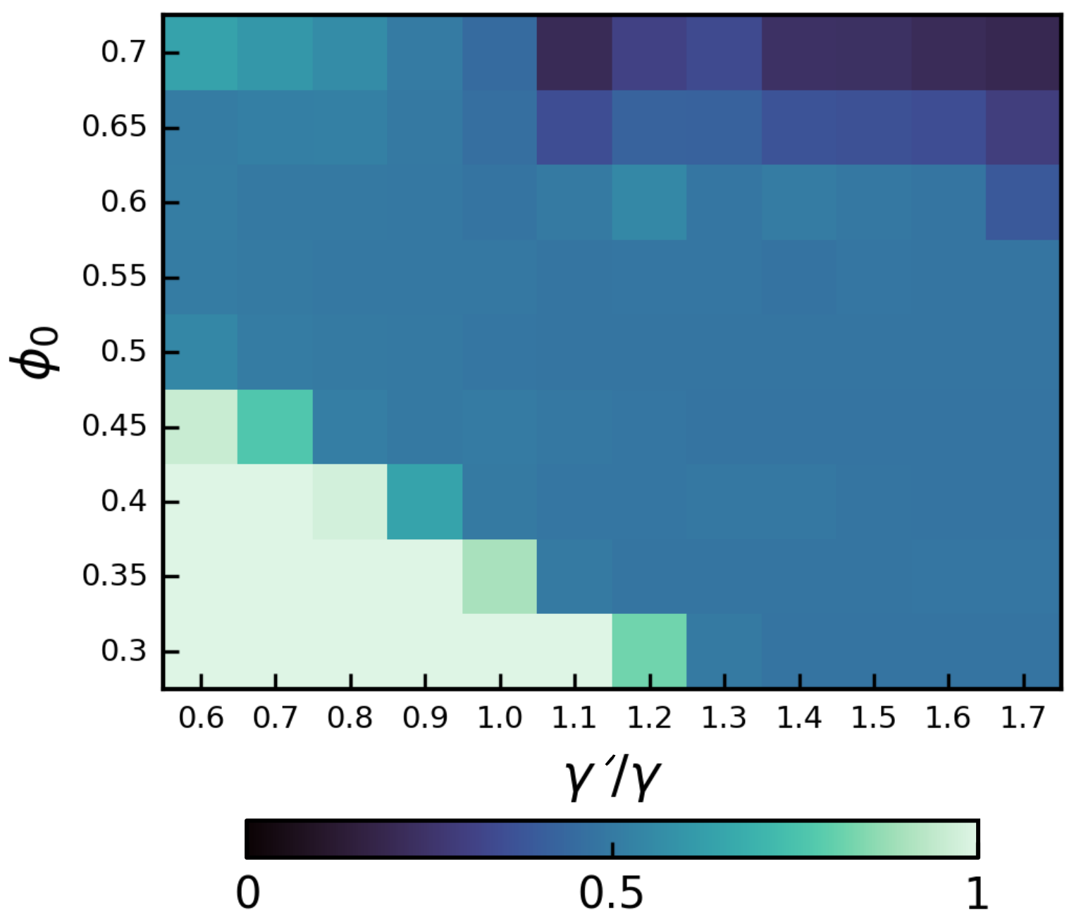
Figure 2: State diagram of the $\alpha$ exponent in $m(t)\sim t^{\alpha}$ with varying $\phi_{0}$ and $\gamma^{\prime}/\gamma$, in a system with $c_{0}=0.5$.

To quantify evaporative dynamics, consider the position of the interface $x_{\rm i}$, taken to be the position of the peak in $c(t)$. Fig. 1c shows a log-log plot of $\Delta x_{\rm i}(t)=x_{\rm i}(t)-x_{\rm i}(0)=m(t)$ by mass conservation if only solvent leaves the interface. For pure solvent ($c_{0}=0$), $\Delta x_{\rm i}\sim t$, so that $J\sim\mathrm{d}{(\Delta x_{\rm i})}/\mathrm{d}{t}$ is constant, which is a well-known result [15]. A solvent-polymer mixture ($c_{0}=0.5$, with $\phi_{0}=0.35$ and $\gamma^{\prime}/\gamma=1.50$) behaves differently. After an initial linear regime, the evaporation slows down and approaches a steady state where $\Delta x_{\rm i}\sim t^{1/2}$ and $J\sim t^{-1/2}$, as found by experiments [5, 8] and theory [6].

Stability of the DLE Regime.

To assess the relative stability of the $\Delta x_{\rm i}\sim t$ and $\sim t^{1/2}$ regimes and explore the possibility of other forms of scaling, we scan two parameters. The first, $\gamma^{\prime}/\gamma$, regulates the extent to which $c$ reduces the convective evaporation speed $v=-\gamma\nabla(\phi-(\gamma^{\prime}/\gamma)c)$. The second is the solvent concentration outside the droplet, $\phi_{0}$, which governs the evaporative driving force.

For the exponent $\alpha$ in $m(t)\sim t^{\alpha}$, the state diagram in Fig. 2 displays three dynamical regimes separated by relatively sharp boundaries, with $\alpha\approx 1,0.5$ and 0. We identify the DLE regime by $\alpha\approx 0.5$ and observe that it occupies the largest region in the state diagram, and is therefore the most robust. This is consistent with the fact that diffusive dynamics is the behaviour typically reported in experiments to date.

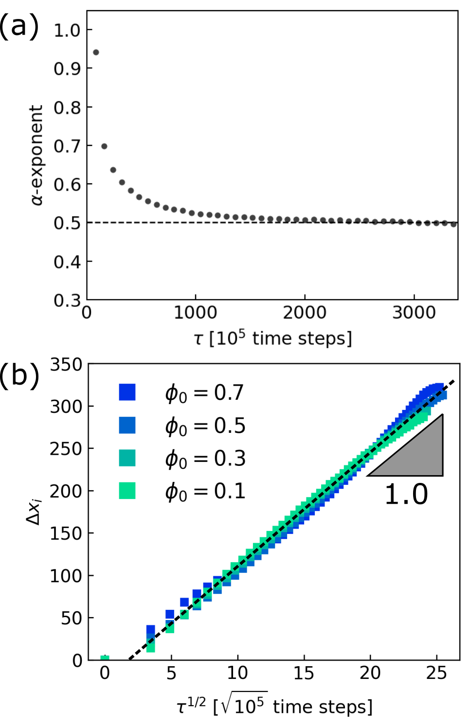
Figure 3: Diffusion-Limited Evaporation (DLE) after long times that is independent of the external driving force. (a) Evolution of the exponent $\alpha$ in $m(t)\sim t^{\alpha}$ over time steps $\tau$ in a system with $\phi_{0}=0.35$ and $\gamma^{\prime}/\gamma=1.5$, settling on a time exponent $\alpha=0.5$. $\alpha$ is found through power law fitting of $m(t)=Bt^{\alpha}$ using $\alpha={\mathrm{d}{\,\ln m(t)}}/{\mathrm{d}{\,\ln t}}$. (b) Evolution of $\Delta x_{\text{i}}$ over the square root of time $\tau^{1/2}$, showing independence of the external driving force $\phi_{0}$. Systems shown are $\phi_{0}=0.7$ with $\gamma^{\prime}/\gamma=0.415$, $\phi_{0}=0.5$ with $\gamma^{\prime}/\gamma=1.00$, $\phi_{0}=0.3$ with $\gamma^{\prime}/\gamma=1.85$ and $\phi_{0}=0.1$ with $\gamma^{\prime}/\gamma=2.75$.

To understand the stability of the $\Delta x_{\rm i}\sim t^{1/2}$ regime, note that Eqs. 1 become diffusion equations in the limit $v\to 0$ [6]. The system cannot start in this regime, but can only approach it asymptotically: having $\gamma^{\prime}/\gamma\sim\nabla_{\rm i}\phi/\nabla_{\rm i}c$ to give $v\to 0$ (where $\nabla_{\rm i}\equiv$ gradient at the interface) means no evaporation in the first place. We therefore need $\gamma^{\prime}/\gamma\lesssim\nabla_{\rm i}\phi/\nabla_{\rm i}c$ to confer a finite initial evaporation rate, which then decreases with time as interfacial polymer accumulates and the system approaches the diffusive regime ($\alpha=0.5$) asymptotically, Fig. 3a. How fast this happens depends on the effectiveness of interfacial polymer in reducing evaporation, which is controlled by $\gamma^{\prime}$.

As $\gamma^{\prime}/\gamma$ drops, this effectiveness decreases, requiring a larger polarisation layer that takes longer to establish to approach the diffusive regime. So, for finite system size and observation time, there exists a $(\gamma^{\prime}/\gamma)_{\rm min}=\epsilon$ below which the system will not cross over to $\Delta x_{\rm i}\sim t^{1/2}$ behaviour. We expect $\epsilon$ to increase with the polymer mobility, $M_{\rm c}$: more mobile polymers requires longer time to build up a large enough polarisation layer to slow evaporation. On the other hand, a stronger driving force for evaporation due to lower external solvent concentration, $\phi_{0}$, requires the polymer to be more effective in reducing evaporation for diffusive behaviour to emerge; so, $\epsilon$ should decrease with increasing $\phi_{0}$, as observed, Fig. 2.

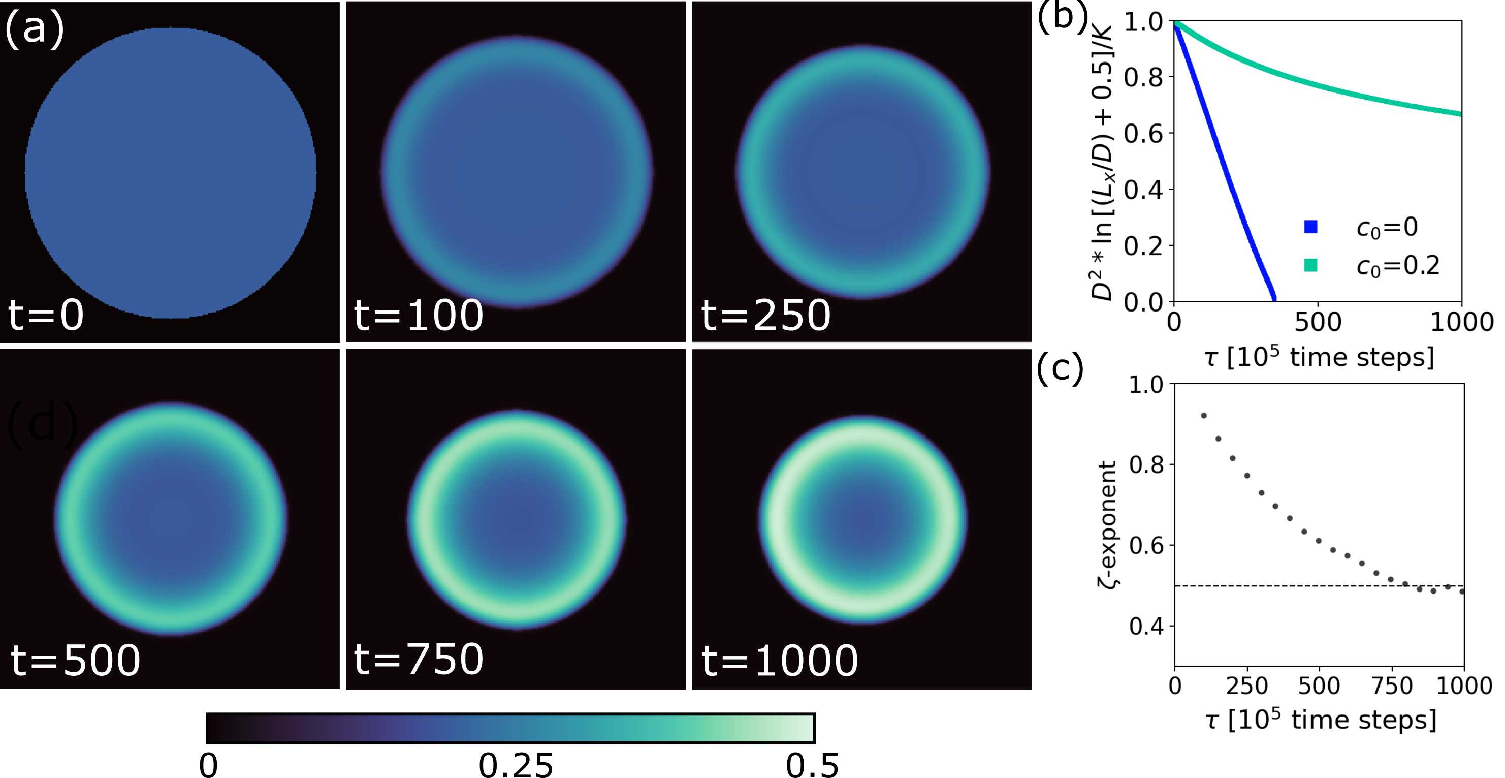
Figure 4: Dynamic evolution of evaporating droplets in 2D. (a) Snapshots of the time evolution of polymer concentration $c$ in a 2D evaporating droplet, with $c_{0}=0.2$, $\phi_{0}=0.35$ and $\gamma^{\prime}/\gamma=3.0$. (b) Evolution of the log-corrected area $D^{2}\ln{[(L_{\text{x}}/D)+0.5]}/G$ of the system in (a) plotted over time, comparing a system with added polymer to a system of pure solvent. (c) Evolution of the exponent $\zeta$ in $D^{2}\ln{[(L_{\text{x}}/D)+0.5]}\sim t^{\zeta}$ over timesteps $\tau$ in a system with $\phi_{0}=0.35$ and $\gamma^{\prime}/\gamma=3.0$, settling on a time exponent $\zeta=0.5$. $\zeta$ is found through power law fitting using $\zeta={\mathrm{d}\ln{\left[1-(D^{2})\ln{[(L_{\text{x}}/D)+0.5]}/G\right]}}/{\mathrm{d}\ln{t}}$.

To understand the physics underpinning the late-stage, diffusive regime, note that by this stage, the chemical potential of the solvent (at partial pressure $p$) just inside the interface (where the polarisation layer is at its most concentrated), $\mu(p)|_{{x}_{\text{i}}}$, has nearly equilibrated with that of the solvent vapour outside, and so is nearly constant. At the same time, the solvent chemical potential in the middle of the droplet, $\mu(p)|_{{x}=0}$, is also constant. So, there is a constant osmotic pressure difference driving solvent flow through the polarisation layer towards the interface, $\Delta p=p|_{{x}_{\text{i}}}-p_{{x}=0}<0$ (because $\mu(p)|_{x_{\rm i}}<\mu(p)|_{{x}=0}$). Treating the growing polarisation of thickness $L(t)$ as a porous medium of Darcy permeability $k$ implies the solvent flux $J=-\frac{k}{\eta L(t)}\Delta p$, with $\eta$ the solvent viscosity. In the DLE regime in steady state, this flux is exactly balanced by the evaporative flux, which mass conservation requires to be $\mathrm{d}{L}/\mathrm{d}{t}$, so that we have $\mathrm{d}{L}/\mathrm{d}{t}\sim L^{-1}$, or $L(t)\sim t^{1/2}$, as also found in a recent theory [16] as well in our numerics (see SI II.A). Darcy’s law then implies $J\sim t^{-1/2}$, consistent with our finding that $\Delta x_{\rm i}\sim t^{1/2}$ at long times (recall that $J\sim\mathrm{d}{(\Delta x_{\rm i})}/\mathrm{d}{t}$), Fig. 1c.

For this physical argument to hold, we require that the rate of advective polymer accumulation, giving rise to the (growing) polarisation layer, dominates polymer diffusion which counteracts this buildup, i. e. the Péclet number $\mathrm{Pe}\equiv\frac{vL(t)}{M}\gg 1$. While this is true at short times, it seems at least at first sight that this condition will be broken as late times where naïvely one might expect $\mathrm{Pe}\to 0$ as $v\to 0$. However, in the DLE regime, our argument suggests $v\sim\dot{m}(t)\sim t^{-1/2}$, $L(t)\sim t^{1/2}$. So in fact at late times $\mathrm{Pe}\sim t^{0}$, provided that $M_{\text{c}}=\frac{M_{0}}{1+\beta c}\simeq\mathrm{constant}$. The latter is a fair approximation for systems with $\beta\sim 0.1$–1.0 and $c\sim 0.1$–1.0. Our physical argument for the diffusive regime at long time is therefore self consistent, because the balance between advection and diffusion remains constant even as $v\to 0$. For a final check, we find $\mathrm{Pe}\approx 10^{2}\gg 1$ for a typical system in the DLE regime ($\gamma^{\prime}/\gamma=1.50$, $\phi_{0}=0.30$), so that, indeed, advection near the interface dominates over diffusion.

In the diffusive regime, it was previously predicted [6] that the mass loss rate should be independent of the external driving force. For water evaporation into air, the driving force is the relative humidity $a_{e}$ [15], which for us is ‘tuned’ by $\phi_{0}$. Plotting $m$ vs $t^{1/2}$ whilst varying $\phi_{0}$ and $\gamma^{\prime}/\gamma$, Fig. 3b, shows that this is indeed the case in our model.

This is a direct consequence of the fact that interfacial polymer concentration has reached a constant value, $c_{\rm{g}}$, so that it is the polymer concentration gradient in the polarisation layer rather than the external humidity that drives water transport. In the theory of Salmon et al [6], the same physics emerges due to the sharp fall in water activity at high polymer concentrations, so that the late stage interfacial polymer concentration varies very little over a broad range of external water activities. In both cases, the humidity independence is necessarily correlated with the emergence of DLE. However, such correlation is not logically necessary. In our earlier experiments, the formation of a thin polymer skin at the solution-air interface due to rapid adsorption also gives rise to humidity-independent evaporation, but without a porous polarisation layer, the dynamics is not diffusive [8].

Extensions of the Model to more Complex Systems.

One of the major advantages of our phase field model is the ease with which it can adapted to more complex systems and used to explore higher dimensions. Fig. 4a shows the evolution of a 2D evaporating drop geometry for a system with $c_{0}=0.2$, $\phi_{0}=0.35$ and $\gamma^{\prime}/\gamma=3.0$. As in 1D, a concentrated polymer layer forms at the solvent-air interface over time.

For 2D or 3D droplets of diameter $D$ evaporating in an unconfined environment, $D^{2}\sim t$, so that the evaporation rate is constant [17]. However, solving the same problem in a confined system with a constant solvent chemical potential imposed at the system’s boundary leads to deviations from this ‘$D^{2}$ law’. If viscous and buoyancy effects can be neglected, theory [17] predicts that in a 2D finite system of this kind,

$$D^{2}\ln{[(L_{\text{x}}/D)+0.5]}/G=1-Ct\,,$$ (3)

where $L_{x}$ is the size of one axis of the system, $C$ is a constant and $G=D_{0}^{2}\ln{[(L_{\text{x}}/D_{0})+0.5]}$. Over the course of the simulations that give the results shown in Fig. 4, the solvent concentration at the (periodic) boundaries increases by $\lesssim 2\%$, so that we may expect Eq. 3 to hold to a good approximation.

Our data for the evaporation of a pure solvent droplet, Fig. 4b, (blue; $c_{0}=0$) indeed agree with Eq. 3, as apparent from the approximately linear evolution of $D^{2}\ln{[(L_{\text{x}}/D)+0.5]}/G$ with $t$. However, in a system with added polymer, deviations are observed, Fig. 4b (green, $c_{0}=0.2$), which recall Fig. 1c. We therefore fit these data to a power law with a running exponent $\zeta$, $D^{2}\ln{[(L_{\text{x}}/D)+0.5]}\sim t^{\zeta}$. The resulting $\zeta$, Fig. 4c, clearly recalls Fig. 3a for the 1D case.

So, while a full study of the 2D case is beyond our scope, it seems reasonable to surmise that the state diagram in this case should also display a robust diffusive regime, provided that $\mathrm{Pe}$ is high enough. Previous experiments have demonstrated ambient humidity independent evaporation of droplets containing large glycoproteins [18], which is consistent with our surmise.

Conclusions and Outlook

In summary, we have used a phase field model to study the evaporative dynamics of a polymer-solvent mixture. Our key result is that the DLE regime, where the evaporation rate decays with time as $t^{-1/2}$, is a robust dynamical regime found over a range of parameter values. We rationalise this scaling with a simple mathematical and physical argument, according to which the $-1/2$ exponent is due to a diffusive growth of the polymer layer, and a Darcy flow of the solvent due to the ensuing pressure difference close to the solvent-air interface. For this argument to be self-consistent, the Péclet number $\mathrm{Pe}$ should remain high and nearly constant, to achieve a non-equilibrium steady state where advection dominates over diffusion at all times. We show that this requirement is, perhaps surprisingly, indeed met.

Our model is in quantitative agreement with previous theoretical and experimental results, including a near-independence of evaporation rates on relative humidity in the DLE regime. Such agreement gives confidence for applying this phase field model to study solvent and solute transfer in more complex systems and geometries. We have shown preliminary results for the evaporation of a 2D droplet to demonstrate this potential. Possible future application include dissolution processes (e. g., making instant coffee) and the drying of multilayers involving multiple solvents and solutes (e. g., oil paintings [19]). In the latter case, our approach has the added advantage that no assumptions need to be made on the phase of layers and/or the location of the interface over time.

References

Supplemental Information: Diffusive evaporation dynamics in polymer solutions is ubiquitous

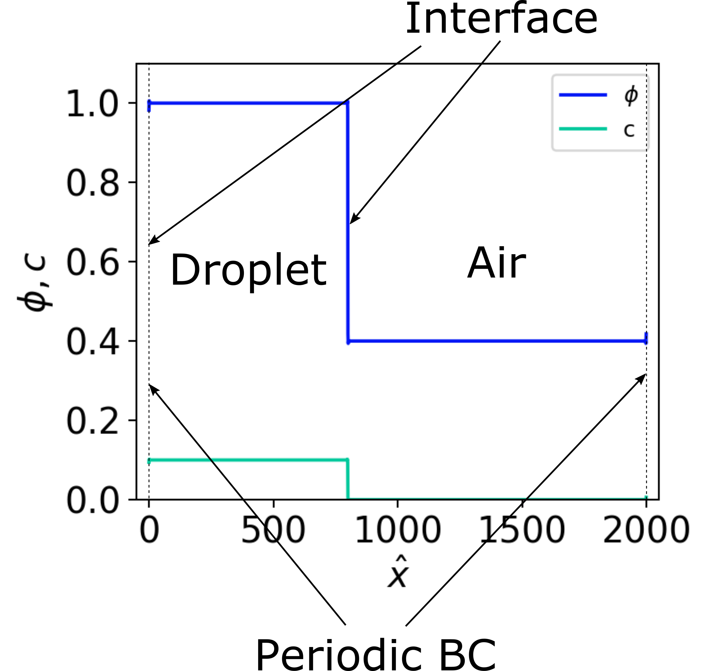
Figure S1: Initialized one dimensional system, where $\phi$ and $c$ are divided over lattices in $x$. The droplet and the surrounding air phases are separated by a continuous interface. Here $2/5$ of the system is droplet and the remainder is air.

SI Analytical model

SI.1 Set-up of the Analytical System

For the binary polymer-water system we create two fields, one for the solvent concentration $\phi$ and one for the polymer concentration $c$, discretized over the same lattice system so that each lattice contains some finite value of $\phi$ and $c$.

We initialize a system with two phases, the droplet and the surrounding air, separated by a continuous interface, see for example a one-dimensional system in Fig. S1. In phase 1, inside the droplet, we set the solvent concentration to $\phi=\phi_{1}$ ($=1$), and the polymer concentration $c$ to some other finite value $c=c_{0}$, where $c_{0}<\phi_{1}$. In phase 2, the surrounding air, we set the solvent concentration to $\phi=\phi_{0}$ with $\phi_{0}<\phi_{1}$, which represents the Relative Humidity (RH). Also, there should be no polymer in the air phase ($c=0$).

We note that the system is slightly compressible, due to an increase of $c$ inside the drop. However, since the total concentration of material (polymer and solvent) is equal to $\phi+Ac$, where $A$ is a proportionality constant which is not strictly defined in our model, we may safely assume that the compressibility is negligible.

Since the amount of solvent in the air phase should not significantly increase during a simulation, as in reality would also not happen to the environment during evaporation, we can safely allow $\phi$ is not to be conserved in the surrounding phase.

Furthermore, we used periodic boundary conditions, which means in the case of the one-dimensional droplet there are two interfaces between the droplet and the air.

SI.2 Applying Cahn-Hilliard to Evaporation of a Binary Polymeric Mixture

We start from the general Cahn-Hilliard expression for the solvent concentration $\phi$ and add a convective term to account for the advective flux driven by evaporation, similar to [12]. We define the phase field for $\phi$ follows:

$$\frac{\partial\phi(x,t)}{\partial t}+\nabla\cdot(v\phi)=M_{\phi}\nabla\cdot\left[\nabla\frac{\delta F}{\delta\phi(x)}\right]\,.$$ (S1)

In this form, the second term om the left is a divergence, and ensures conservation of the total amount of solvent. However, in our simulations, solvent is not conserved, because $\phi\sim~{}$constant in the air phase. We therefore replace $\nabla\cdot(v\phi)$ by $v\cdot\nabla\phi$. We express the evaporation rate as an advective term that links the fields for $\phi$ and $c$ as $v=-\gamma\nabla(\phi-\frac{\gamma^{\prime}}{\gamma}c)$, where $\gamma^{\prime}$ and $\gamma$ are kinetic parameters. $\gamma$ gives the relative importance of the convective term and the ratio $\frac{\gamma^{\prime}}{\gamma}$ gives the extent to which the polymer reduces the evaporation rate. Also, we take that $\frac{\delta F}{\delta\phi}=\mu_{\phi}$ and that the solvent has a constant mobility $M_{\phi}$. This leads to the following governing equation for the phase field of the solvent:

$$\frac{\partial\phi(x,t)}{\partial t}+v\cdot\nabla(\phi)=M_{\phi}\nabla^{2}\mu_{\phi}\,.$$ (S2)

We also require an equation for the phase field of the polymer, which reads similarly:

$$\frac{\partial c(x,t)}{\partial t}+\nabla\cdot(vc)=\nabla\cdot(M_{c}(c)\nabla\mu_{c})\,,$$ (S3)

where we assume that $c$ is conserved in the droplet and that the mobility of the polymer is be concentration dependent as $M(c)=\frac{M_{0}}{1+\beta c}$.

Note that, as previously mentioned, we interpret $\phi$ and $c$ as solvent and polymer concentration respectively. Another mathematically consistent interpretation is to take the phase field $\phi$ as total mass inside the droplet (polymer plus solvent): in this case the droplet would remain incompressible, and we would be approximating the evaporation velocity with the gradient of the water density (which would be $\phi-\frac{\gamma^{\prime}}{\gamma}c$ in this interpretation).

SI.3 Free Energy Density and Chemical Potentials

To obtain the diffusive term we calculate the chemical potentials as functional derivatives of the free energy density, that depends on the local values of $\phi$ and $c$:

$$\mu_{\phi} =\frac{\delta F}{\delta\phi}=\frac{\partial f}{\partial\phi}-\nabla\cdot\frac{\partial f}{\partial\nabla\phi}\,,$$ (S4a)

$$\mu_{c} =\frac{\delta F}{\delta c}=\frac{\partial f}{\partial c}-\nabla\cdot\frac{\partial f}{\partial\nabla c}\,.$$ (S4b)

We start from the following functional form for $f$:

$$\begin{split}f=\frac{a_{1}}{4}(\phi-\phi_{0})^{2}(\phi-\phi_{1})^{2}+\frac{\kappa_{\phi}}{2}(\nabla\phi)^{2}+\frac{\kappa_{c}}{2}(\nabla c)^{2}\\[3.0pt] &{}-\frac{a_{0}}{2}\phi^{2}c^{2}+\frac{b_{0}}{2}c^{2}+\frac{b_{1}}{4}c^{4}\,,\end{split}$$ (S5)

Here, the first term $\frac{a_{1}}{4}(\phi-\phi_{0})^{2}(\phi-\phi_{1})^{2}$ drives phase separation into two phases of compositions $\phi_{1}$ and $\phi_{0}$ ; the second and third terms $\frac{\kappa_{\phi}}{2}(\nabla\phi)^{2}$ and $\frac{\kappa_{c}}{2}(\nabla c)^{2}$ give the bare surface tension of $\phi$ and $c$ ; the fourth term $\frac{a_{0}}{2}\phi^{2}c^{2}$ accounts for the solvent-polymer interaction, which is negative as it should lower the free energy (good solvent condition); the fifth term $\frac{b_{0}}{2}c^{2}$ represents the virial coefficient for polymer diffusion; and the final term $\frac{b_{1}}{4}c^{4}$ is the excluded volume interaction of the polymer.

SI.4 Energy Penalty for Polymer Evaporation

The phase field model as outlined in the above is purely interaction based through the free energy density equation. Since polymer and solvent have affinity, in the current form of Eq. S5 polymer will ‘leak’ into the outer phase. This is not physically unrealistic in liquid-liquid systems, but will become an issue when there is a phase change over the interface like in a gas-liquid system.

In a gas-liquid system, solvent molecules are easily transferred to the gas phase, e. g. this does not require much energy. Thus, the energy contribution for $\phi$ to cross the interface and move from liquid to gas can be safely ignored in Eq. S5.

The solute is involatile and unlikely to evaporate, so there should be an energy penalty for $c$ to cross the interface to the outer phase $\phi_{0}$. This can be implemented by adding a term $\theta(x)\frac{a_{\text{2}}}{2}c^{2}$ to our free energy density so that it becomes

$$\begin{split}f(\phi,c)&=\frac{a_{1}}{4}(\phi-\phi_{0})^{2}(\phi-\phi_{1})^{2}+\frac{\kappa_{\phi}}{2}|\nabla\phi|^{2}\\[3.0pt] &\hskip 10.00002pt{}+\frac{\kappa_{c}}{2}|\nabla c|^{2}-\frac{a_{0}}{2}\phi^{2}c^{2}+\theta(x)\frac{a_{\text{2}}}{2}c^{2}\\[3.0pt] &\hskip 10.00002pt{}+\frac{b_{0}}{2}c^{2}+\frac{b_{1}}{4}c^{4}\end{split}$$ (S6)

where $\theta(x)=\Theta(\phi-\frac{\phi_{1}-\phi_{0}}{2})$ is an indicator function which is zero if $\frac{\phi_{1}-\phi_{0}}{2}>\phi$ and one otherwise, and $a_{\rm{2}}$ is the energy penalty (units $E/L^{2}$) for the polymer to be in the outer phase.

SI.5 Concentration Cap

When $c$ increases to some concentration $c=c_{g}$, the polymer gels and contributes a permanent elastic stress to the system [14, 10]. This effect can be implemented into the free energy by adding a term $\theta^{\prime}(x)\frac{K_{\text{g}}}{2}(c-c_{\text{g}})^{2}$, which now becomes

$$\begin{split}f(\phi,c)=\frac{a_{1}}{4}(\phi-\phi_{0})^{2}(\phi-\phi_{1})^{2}+\frac{\kappa_{\phi}}{2}|\nabla\phi|^{2}+\frac{\kappa_{c}}{2}|\nabla c|^{2}\\[3.0pt] &{}-\frac{a_{0}}{2}\phi^{2}c^{2}+\theta(x)\frac{a_{\text{2}}}{2}c^{2}+\theta^{\prime}(x)\frac{K_{\text{g}}}{2}(c-c_{\text{g}})^{2}\\[3.0pt] &{}+\frac{b_{0}}{2}c^{2}+\frac{b_{1}}{4}c^{4}\,,\end{split}$$ (S7)

where $\theta^{\prime}(x)=\Theta(c-c_{\rm{g}})$ is another indicator function which is zero if $c<c_{\rm{g}}$ and one otherwise, and $K_{\rm{g}}$ (units $E/L^{2}$) is the osmotic bulk modulus in the gel phase.

SI.6 Chemical Potential Expressions

The chemical potentials used in the diffusive term read as follows:

$$\begin{split}\mu_{\phi}=\frac{\partial f}{\partial\phi}-\nabla\cdot\frac{\partial f}{\partial\nabla\phi}\\[3.0pt] &{}=a_{1}(\phi-\phi_{0})(\phi-\phi_{1})(\phi-\frac{\phi_{0}+\phi_{1}}{2})\\[3.0pt] &{}-a_{0}c^{2}\phi-\kappa_{\phi}\nabla^{2}\phi\,,\end{split}$$ (S8)

$$\begin{split}\mu_{c}=\frac{\partial f}{\partial c}-\nabla\cdot\frac{\partial f}{\partial\nabla c}\\[3.0pt] &{}=-a_{0}c\phi^{2}+b_{0}c+\theta(x)a_{\rm{2}}c+b_{1}c^{3}\\[3.0pt] &{}+\theta^{\prime}(x)K_{\rm{g}}(c-c_{\rm{g}})-\left[\kappa_{c}\nabla^{2}c\right]\,.\end{split}$$ (S9)

SI.7 Parameter values

Since the phase field is not restricted by classical physics, we need to choose all phenomenological parameters such that the system behaves realistically. The set of parameters that was used in our simulations for the free energy and the conservation equations, in units of $E$ (energy $\delta E$), $L$ (length $\delta x$) and T (time $\delta t$), is given in Table 1.

Table 1: Parameter values used in simulations.

Parameter	Units	Value
$a_{1}$	$E/L^{2}$	1.0-3.0
$\kappa_{\phi}$	$E$	0.1
$\kappa_{c}$	$E$	0.1-0.4
$a_{0}$	$E/L^{2}$	0.02
$b_{0}$	$E/L^{2}$	0.001-0.03
$b_{1}$	$E/L^{2}$	0.001
$\gamma$	$L^{2}/T$	0.0001
$\gamma^{\prime}$	$L^{2}/T$	0.00005-0.0003
$M_{\phi}$	$L^{2}/ET$	0.1
$M_{0}$	$L^{2}/ET$	0.025-0.1
$\beta$	-	0.5-5.0
$a_{\rm{2}}$	$E/L^{2}$	0.5
$K_{\rm{g}}$	$E/L^{2}$	0.5
$c_{\rm{g}}$	-	0.5-1.0

SII Analysis of Results

SII.1 Evaporation Rate and Growth of Polymer Layer

During evaporation in an incompressible system, the total density $\rho_{\rm{tot}}=\phi+c$ cannot increase at a lattice in the droplet. Thus, the loss of $\phi$ needs to be proportional the build-up of $c$ in the drop. After the polymer concentration at the interface has reached $c=c_{\rm{g}}$, the polymer layer grows inward as it is swept up by the shrinking interface into the droplet as water molecules diffuse outwards to evaporate. This leads to the proportionality $L(t)\sim-m(t)$, where $L(t)$ is the Full Width Half Maximum (FWHM) of the peak in $c$ near the interface and $m(t)$ is the mass loss (a minus is added because mass is lost from the droplet).

To test this proportionality we look at the exponents of the mass loss, e.g. the interface shrinkage $\Delta x_{\rm{i}}$, $m(t)\sim\Delta x_{\rm{i}}\sim t^{\alpha}$ and the polymer layer growth $L(t)\sim t^{\beta}$ in an evaporating droplet where the polymer reaches its capping/gel concentration early in the simulation (Fig. S2). We determine the time exponents $\alpha=0.56$ and $\beta=0.60$ by power-law fitting, which is indeed similar.

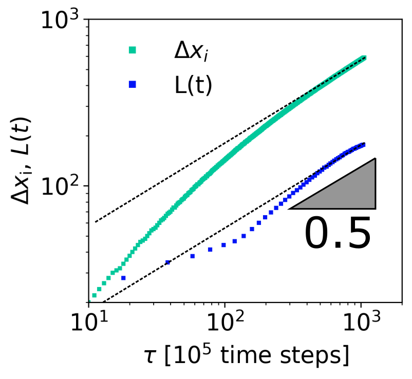
Figure S2: Comparison of the evolution of the interface $\Delta x_{\rm{i}}$ and the polymer layer thickness $L(t)$ in a system with $\gamma^{\prime}/\gamma=1.5$ and $\phi_{0}=0.35$, plotted logarithmically to highlight the long time power-law behaviour. The capping concentration is reached after approximately $t=100$ timesteps.

References

- [1] BJD Gans, US Schubert, Inkjet printing of well-defined polymer dots and arrays. Langmuir 20, 7789–7793 (2004).
- [2] Z Erbay, F Icier, A review of thin layer drying of foods: Theory, modeling, and experimental results. CRC Crit. Rev. Food Sci. 50, 441–464 (2010).
- [3] MG Hennessy, GL Ferretti, JT Cabral, OK Matar, A minimal model for solvent evaporation and absorption in thin films. J. Coll. Interf. Sci. 488, 61–71 (2017).
- [4] PG de Gennes, Solvent evaporation of spin cast films: “crust” effects. Eur. Phys. J. E 7, 31–34 (2002).
- [5] K Roger, M Liebi, J Heimdal, QD Pham, E Sparr, Controlling water evaporation through self-assembly. Proc. Natl. Acad. Sci. (USA) 113, 10275–10280 (2016).
- [6] JB Salmon, F Doumenc, B Guerrier, Humidity-insensitive water evaporation from molecular complex fluids. Phys. Rev. E 96, 032612 (2017).
- [7] M Rezaei, RR Netz, Water evaporation from solute-containing aerosol droplets: Effects of internal concentration and diffusivity profiles and onset of crust formation. Phys. Fluids 33, 091901 (2021).
- [8] M Huisman, P Digard, WCK Poon, S Titmuss, Evaporation of concentrated polymer solutions is insensitive to relative humidity. Accepted in Phys. Rev. Lett. (2023).
- [9] K Ozawa, T Okuzono, M Doi, Diffusion process during drying to cause the skin formation in polymer solutions. Japan. J. Appl. Phys. 45, 8817–8822 (2006).
- [10] T Okuzono, M Doi, Effects of elasticity on drying processes of polymer solutions. Phy. Rev. E 77, 030501(R) (2008).
- [11] K Roger, JJ Crassous, How the interplay of molecular and colloidal scales controls drying of microgel dispersions. Proceedings of the National Academy of Sciences 118, e2105530118 (2021).
- [12] HG Lee, J Yang, S Kim, J Kim, Modeling and simulation of droplet evaporation using a modified Cahn–Hilliard equation. Appl. Math. Comput. 390, 125591 (2021).
- [13] M Kardar, G Parisi, YC Zhang, Dynamic scaling of growing interfaces. Phys. Rev. Lett. 56, 889–892 (1986).
- [14] L Leibler, K Sekimoto, On the sorption of gases and liquids in glassy polymers. Macromol. 26, 6937–6939 (1993).
- [15] EL Cussler, Diffusion : Mass Transfer in Fluid Systems. (CUP, Cambridge, UK), (1997).
- [16] L Talini, F Lequeux, Formation of glassy skins in drying polymer solutions: approximate analytical solutions. Soft Matter 19, 5835–5845 (2023).
- [17] L Fei, et al., Droplet evaporation in finite-size systems: Theoretical analysis and mesoscopic modeling. Phys. Rev. E 105, 025101 (2022).
- [18] EP Vejerano, LC Marr, Physico-chemical characteristics of evaporating respiratory fluid droplets. J. Roy. Soc. Interface 15, 20170939 (2018).
- [19] JR Duivenvoorden, et al., The distribution and transport of water in oil paintings: A numerical moisture diffusion model. Int. J. Heat Mass Tran. 202, 123682 (2023).