Multinomial belief networks

Abstract

A Bayesian approach to machine learning is attractive when we need to quantify uncertainty, deal with missing observations, when samples are scarce, or when the data is sparse. All of these commonly apply when analysing healthcare data. To address these analytical requirements, we propose a deep generative model for multinomial count data where both the weights and hidden units of the network are Dirichlet distributed. A Gibbs sampling procedure is formulated that takes advantage of a series of augmentation relations, analogous to the Zhou-Cong-Chen model. We apply the model on small handwritten digits, and a large experimental dataset of DNA mutations in cancer, and we show how the model is able to extract biologically meaningful meta-signatures in a fully data-driven way.

I Introduction

Maximum likelihood methods are prone to overtraining, and do not make optimal use of data. Although these issues are inconsequential when sufficient training data is present, when training data is limited, many machine learning methods including deep neural networks often do not give optimal results [1]. In addition, these methods do not naturally model situations where missing data or uncertainty is important [2, 3].

Another class of methods use probabilistic or fully Bayesian methods to model data. Examples include latent Dirichlet allocation[4], deep belief nets [5, 6], and variational autoencoders [7]. In principle, Bayesian methods make optimal use of training data as well as guard against overtraining, account for uncertainty, and deal with missing data in a principled way. However, current approaches fall short of the ideal in different ways. One class of methods use variational methods to enable learning, which involve approximations that partially undo the advantages of a Bayesian approach. Some methods use exact sampling, but are limited in their representational power by using binary variables [5] or use Poisson-distributed variables as output [6].

Here we introduce a Bayesian deep belief network that uses multinomial-distributed variables as output. The multinomial distribution is a versatile choice for a range of data types encountered in practice. For instance, in combination with the bag-of-words approximation it is commonly used to model text documents, and it is an obvious choice for categorical and binary variables appearing in questionnaires and health data. Using augmentation techniques both real-valued and ordinal data can be modelled as well. Importantly, it is straightforward to model several multinomials simultaneously (each with its own dimension and observation count) which naturally enables modeling heterogeneous data, while missingness is accounted for by allowing some multinomial observations to be absent. We will develop those extensions elsewhere; here we focus on modeling a single multinomial-distributed observation.

A prominent example of a model with multinomial output variables is Latent Dirichlet Allocation (LDA) [4]. In one representation of the model, it factorizes the latent parameter matrix of the multinomial distributions across samples as a low-rank product of (sample-topic and topic-feature) matrices whose rows are drawn from Dirichlet distributions. The low-rank structure, the sparsity induced by the Dirichlet priors, and the existence of effective inference algorithms have resulted in numerous applications and extensions of LDA. Despite this success, LDA has some limitations. One is that inference of the Dirichlet hyperparameters is often ignored or implemented using relatively slow maximum likelihood methods [8, 9]. This was elegantly addressed by [10] by endowing the Dirichlet distribution with another Dirichlet prior in a hierarchical structure, allowing information to be borrowed across samples. Another limitation is that LDA ignores any correlation structure among the topic weights across samples, which for higher latent (topic) dimensions becomes increasingly informative. An effective approach that addresses this issue was developed by [6], who developed a multi-layer fully-connected Bayesian network using gamma variates and Poisson, rather than multinomial, observables. Here we aim to extend and combine these two approaches in the context of multinomial observations, resulting in a model whose structure resembles a fully connected multi-layer neural network and that retains the efficient inference properties of LDA.

This paper is structured as follows. We first briefly position our approach in the context of earlier work. In section III we review the PGBN and introduce our model in IV. The model is applied to handwritten digits and mutations in cancer in Sec. V. Finally, a brief summary and outlook are given in the Discussion and Conclusion (Sec. VI).

II Relation to previous work

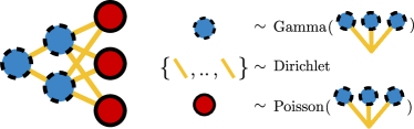
(a)

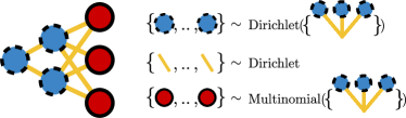
(b)

Figure 1: Schematic representation of the two belief networks. Red nodes are observations, blue dashed circles are latent hidden units, and edges are latent weights. (a) Poisson gamma belief network. (b) Multinomial belief network.

This work focuses on all aspects of (parametric) model uncertainty. Most previous work studied uncertainty in the global parameters (e.g., the weights and biases), such as in Bayesian deep learning [11]. Uncertainty in the local parameters (e.g., the hidden units) has received comparatively little attention. Here, we focus specifically on low-rank factorisation algorithms of features (as opposed to graphs, such as stochastic block models [12]).

From the posterior inference perspective, previous work can be categorised into three approaches. First, several authors use variational inference (VI) to infer the posterior of (deep) topics models composed of, typically, distributions within the exponential family [13, 14, 15, 16]. Variational inference, which solves the inference problem through optimisation, has the advantage that it can be scaled to large datasets. However, since VI operates on a lower bound, there is no guarantee that the posterior is recovered [17]. Second, Markov chain Monte Carlo was used in the gamma belief networks of Zhou et al. [6], Dirichlet belief network of Zhao et al. [18], the multi-label model of Panda et al. [19], and in this paper. In principle, samples from the exact posterior are obtained assuming that the sampler is run to convergence. Sampling-based approaches are however challenging to scale to large datasets: a pass over the entire dataset is needed for each step. Finally, the third approach considers a middle ground. For example, stochastic gradient MCMC (SG-MCMC) [20] was used to do inference in the PGBN [21]. Hybrid approaches, such as the autoencoder in Refs. [22, 23] and the deep diverse LDA model [24] combine SG-MCMC with VI to infer the posterior.

In terms of model architecture, the generative model proposed here is similar to the deep exponential family [13]. We closely follow the Poisson-gamma belief network (PGBN) introduced by [6]. However, we differ from that work in that we start with observations that are multinomial instead of Poisson distributed (Fig. 1). Thus, the total number of observations per example is fixed (i.e., conditioned on) instead of part of the model, allowing us to naturally model missingness. In particular, we too use Dirichlet distributions to model the connections between layers, but instead of gamma distributions, we again use Dirichlet distributions to represent internal activations. Other works considered tree-structured [25] or hierarchical [18] priors on the latent topic-feature variables. Another difference with the PGBN is that we modulate the overall activation strength per layer rather than per example and layer, as the activation strength corresponds to the concentration parameter of the Dirichlet distribution which modulates its dispersion, which is a property of the sample as a whole rather than of a single observation.

Gibbs sampling in the PGBN was achieved by augmentation with Poisson counts throughout the network; the posterior is sampled by exploiting an alternative factorization of a joint distribution involving an overdispersed Poisson (the gamma-Poisson or negative binomial distribution). In the proposed model, we use augmentation by multinomial distributed variables instead, and similar to the PGBN case, we end up with overdispersed multinomials (in fact Dirichlet-multinomials), and we achieve posterior sampling by developing an analogous alternative factorization. This factorization effectively separates the overdispersed distribution’s mean and dispersion and represents evidence for these two aspects as a pure multinomial latent observation, and one from a Chinese Restaurant Table (CRT) distribution respectively. This allows us to treat the multinomial variable as an observation generated by the layer above so that the process can continue upwards, while we obtain the posterior of the CRT governing the dispersion for this layer using techniques introduced by [26] and [10].

III Poisson gamma belief network

III-A Generative model

We first review the Gamma belief network of Zhou et al. [6] in some detail. The backbone of the model is a stack of Gamma-distributed hidden units $\theta^{(t)}_{vj}$ ($K_{t}$ per sample $j$), with the last one parameterizing a Poisson distribution generating observed counts $x_{vj}$, one for each sample $j$ and feature $v$. The generative model is

$$a_{vj}^{(T+1)} =r_{v},$$ (1)

$$\theta^{(t)}_{vj} \sim\operatorname{Gam}(a_{vj}^{(t+1)},{c_{j}^{(t+1)}}), t=T,\ldots,1$$ (2)

$$a_{vj}^{(t)} =\sum_{k=1}^{K_{t}}\phi^{(t)}_{vk}\theta^{(t)}_{kj}, t=T,\ldots,1$$ (3)

$$x_{vj} \sim\operatorname{Pois}(a_{vj}^{(1)}).$$ (4)

For $T=1$ we only have one layer, and the model reduces to Poisson Factor Analysis, $x_{vj}=\operatorname{Pois}([\boldsymbol{\phi\theta}]_{vj})$ [27]. For multiple layers, the features $\boldsymbol{\theta}^{(t+1)}$ on layer $t+1$ determine the shape parameters of the gamma distributions on layer $t$ through a non-negative connection weight matrix $\boldsymbol{\phi}^{(t+1)}\in\mathbb{R}_{+}^{K_{t}\times K_{t+1}}$, so that $\boldsymbol{\phi}^{(t+1)}$ induces correlations between features on level $t$. The rate of $\boldsymbol{\theta}^{(t)}$ is set by $c_{j}^{(t)}\sim\operatorname{Gam}(e_{0},f_{0})$, one for each sample $j$ and layer $t$. By construction, the weights $\boldsymbol{\phi}^{(t)}$ that connect latent states between layers are normalised as $\sum_{v}\phi^{(t)}_{vk}=1$, which is enforced by Dirichlet priors on $\phi_{vk}^{(t)}\sim\operatorname{Dir}(\{\eta_{v}^{(t)}\}_{v})$; here we use curly braces to denote vectors, with the subscript indicating the index variable; we drop the subscript if the index variable is unambiguous. The top-level activation is controlled by $r_{v}\sim\operatorname{Gam}(\gamma_{0}/K_{T},c_{0})$ where hyperparameters $\gamma_{0}$ and $c_{0}$ determine the typical number and scale, respectively, of active top-level hidden units. The lowest-level activations $\boldsymbol{a}^{(1)}$ parameterize Poisson distributions that generate the observed count variables $x_{vj}$ for sample (individual, observation) $j$. This completes the specification of the generative model.

This model architecture is similar to a $T$-layer neural network, with $\boldsymbol{a}^{(t)}$ playing the role of activations that represent the activity of features (topics, factors) of increasing complexity as $t$ increases.

III-B Deep Poisson representation

An alternative and equivalent representation is obtained by integrating out the hidden units $\boldsymbol{\theta}$ and augmenting with a sequence of latent counts $\boldsymbol{x}^{(t+1)}\kern-2.0pt\rightarrow\kern-2.0pt\boldsymbol{m}^{(t)}\kern-2.0pt\rightarrow\kern-2.0pt\boldsymbol{y}^{(t)}\kern-2.0pt\rightarrow\kern-2.0pt\boldsymbol{x}^{(t)}$. Specifically, let $\operatorname{Log}(p)$ be the logarithmic distribution, with probability mass function $\operatorname{Log}(k;p)\propto{p^{k}/k}$ where $0\kern-2.0pt<\kern-2.0ptp\kern-2.0pt<\kern-2.0pt1$, and define $n\sim\operatorname{SumLog}(l,p)$ by $n=\sum_{i=1}^{l}u_{i}$ where each $u_{i}\sim\operatorname{Log}(p)$. Henceforth, underlined indices denote summation, $x_{\underline{j}}:=\sum_{j}x_{j}$. Augmenting each layer with counts $x_{kj}^{(t)}\sim\operatorname{Pois}(q_{j}^{(t)}a_{kj}^{(t)})$, it turns out these can be generated as

$$m_{jk}^{(t)}\sim\operatorname{SumLog}(x_{kj}^{(t+1)},1-e^{-q_{j}^{(t+1)}});\qquad$$

$$\{y_{vjk}^{(t)}\}_{v}\sim\operatorname{Mult}(m_{jk}^{(t)},\{\phi_{vk}^{(t)}\}_{v});\qquad$$

$$x_{vj}^{(t)}:=y_{vj{\underline{k}}}^{(t)},$$

where $q_{j}^{(t+1)}=\ln[{q_{j}^{(t)}+c_{j}^{(t+1)}]-\ln c_{j}^{(t+1)}}$; see [6] and Supplementary Material sections S2-B, S2-C. Starting with $t=T+1$ this shows how to eventually generate the observed counts $x^{(1)}_{vj}$ using only count variables, with all $\boldsymbol{\theta}^{(t)}$ integrated out. The two alternative schemes are shown graphically in Fig. 2.

Figure 2: Two equivalent generative models for a count variable $\boldsymbol{x}^{(1)}$ from the Poisson gamma belief network, using (a) a tower of real-valued latent variables $\boldsymbol{\theta}$, $\boldsymbol{a}$, or (b) latent counts $\boldsymbol{m}$, $\boldsymbol{y}$, $\boldsymbol{x}$. Blunt arrows indicate deterministic relationships. The variable $\boldsymbol{q}^{(1)}$ is a dummy and has a fixed value $1$. In representation (a) the grayed-out counts $\boldsymbol{x}^{(t)}$ and variables $\boldsymbol{q}^{(t)}$, $t>1$, are included for clarity (and have the same distribution as the variables in the right model) but are not used to generate the outcome $\boldsymbol{x}^{(1)}$, and so can be marginalized out.

III-C Inference

At a high level, inference consists of repeatedly moving from the first representation to the second, and back. This is achieved by swapping, layer-by-layer, the direction of the arrows to sample upward $\boldsymbol{x}^{(t)}\rightarrow\boldsymbol{y}^{(t)}\rightarrow\boldsymbol{m}^{(t)}\rightarrow\boldsymbol{x}^{(t+1)}$; these counts are then used to sample $\boldsymbol{\phi}^{(t)}$ and $\boldsymbol{\theta}^{(t)}$, after which the procedure starts again. To propagate latent counts upwards, we use Theorem 1 of Ref. [28]:

$$p(x,m|a,q)= \operatorname{Pois}(x|qa)\operatorname{SumLog}(m|x,1-e^{-q})$$ (5)

$$= \operatorname{NB}(m|a,1-e^{-q})\operatorname{CRT}(x|m,a),$$

to turn $\boldsymbol{m}\rightarrow\boldsymbol{x}$ into $\boldsymbol{x}\rightarrow\boldsymbol{m}$; here $\operatorname{CRT}(x|m,a)$ is the number of occupied tables in a Chinese restaurant table distribution over $m$ customers with concentration parameter $a$, and $\operatorname{NB}(k|r,p)$ is the negative-binomial distribution with $r$ successes of probability $p$. Finally, we use that independent Poisson variates conditioned on their sum are multinomially distributed with probabilities proportional to the individual Poisson rates, to convert $\boldsymbol{y}\rightarrow\boldsymbol{x}$ to $\boldsymbol{x}\rightarrow\boldsymbol{y}$ as well as $\boldsymbol{m}\rightarrow\boldsymbol{y}$ to $\boldsymbol{y}\rightarrow\boldsymbol{m}$. To Gibbs sample the variables, we first make an upward pass from $\boldsymbol{x}^{(1)}\rightarrow\dots\rightarrow\boldsymbol{x}^{(T+1)}$ followed by a downward pass where the multinomial-Dirichlet conjugacy is used to update $\boldsymbol{\phi}^{(t)}$, the gamma-gamma rate conjugacy to update $\boldsymbol{c}^{(t)}$ and the Poisson-gamma conjugacy to update $\boldsymbol{\theta}^{(t)}$ and $\boldsymbol{r}$. Details are provided in the supplement.

IV Multinomial belief network

IV-A Generative model

To model multinomial observations, we replace the Poisson observables with a multinomial and, for each example $j$, we swap out the gamma-distributed hidden activations for Dirichlet samples $\{\theta^{(t)}_{vj}\}_{v}$. The generative model is

$$a_{vj}^{(T+1)} =r_{v},$$ (6)

$$\{\theta^{(t)}_{vj}\}_{v} \sim\operatorname{Dir}(\{c^{(t+1)}a_{vj}^{(t+1)}\}_{v}), t=T,\ldots,1$$ (7)

$$a_{vj}^{(t)} =\sum_{k=1}^{K_{t}}\phi^{(t)}_{vk}\theta^{(t)}_{kj}, t=T,\ldots,1$$ (8)

$$\{x_{vj}\}_{v} \sim\operatorname{Mult}(n_{j},\{a_{vj}^{(1)}\}_{v}).$$ (9)

As before, the weights are Dirichlet distributed $\phi_{vk}^{(t)}\sim\operatorname{Dir}(\{\eta_{v}^{(t)}\}_{v})$ with hyperparameters $\{\eta_{v}^{(t)}\}_{v}$. Different from the PGBN model we choose one $c^{(t)}\sim\operatorname{Gam}(e_{0},f_{0})$ per dataset (and per layer) instead of one per sample $j$, reducing the number of free parameters per sample, and allowing the variance across samples to inform the $c^{(t)}$. Finally we let the top-level activations $r_{v}$ be Dirichlet distributed, $\{r_{v}\}_{v}\sim\operatorname{Dir}(\{\gamma_{0}/K_{T}\}_{v})$ with $\gamma_{0}$ a hyperparameter. This completes the definition of the generative model.

IV-B Deep multinomial representation

Integrating out $\boldsymbol{\theta}^{(t)}$, the generative model can be alternatively represented as a deep multinomial factor model, as follows (Sec. S3-A, Supplementary Material):

$$n_{j}^{(t+1)} \sim\operatorname{CRT}(n_{j}^{(t)},c^{(t+1)});$$ (10)

$$\{x_{kj}^{(T+1)}\}_{k} \sim\operatorname{Mult}(n_{j}^{(T+1)},\{r_{k}\});$$

$$\{m^{(t)}_{kj}\}_{k} \sim\operatorname{Polya}(n_{j}^{(t)},\{x_{kj}^{(t+1)}\}_{k});$$

$$\{y^{(t)}_{vjk}\}_{v} \sim\operatorname{Mult}(m_{jk}^{(t)},\{\phi^{(t)}_{vk}\}_{v});$$

$$x^{(t)}_{vj} =y^{(t)}_{vj{\underline{k}}}.$$

Here underlined subscripts denote summation; and $\operatorname{Polya}(n,\{y_{k}\})$ is the distribution of the contents of an urn after running a Polya scheme: starting with $y_{k}$ balls of color $k$, repeatedly drawing a ball, returning the drawn ball and a new identically colored one each time, until the urn contains $n$ balls. The two representations of the model are structurally identical to the two representations of the PGBN shown in Fig. 2, except that the $q^{(t)}$ are replaced by $n^{(t)}$, and the relationship between neighbouring $n^{(t)}$ are stochastic instead of deterministic.

IV-C Inference

Similar to the PGBN, we reverse the direction of $\boldsymbol{x}^{(t+1)}\rightarrow\boldsymbol{m}^{(t)}\rightarrow\boldsymbol{y}^{(t)}\rightarrow\boldsymbol{x}^{(t)}$ to propagate information upward. To reverse $\boldsymbol{x}^{(t+1)}\rightarrow\boldsymbol{m}^{(t)}$ into $\boldsymbol{m}^{(t)}\rightarrow\boldsymbol{x}^{(t+1)}$ we use the following:

Theorem 1

The joint distributions over $n$, $\{x_{k}\}$ and $\{m_{k}\}$ below, where $a_{\underline{k}}=1$, are identical:

$$p(n,\{x_{k}\},\{m_{k}\}|n_{0},c,\{a_{k}\})=$$ (11)

$$\operatorname{DirMult}(\{m_{k}\}|n_{0},\{ca_{k}\})\left[\prod_{k}\operatorname{CRT}(x_{k}|m_{k},ca_{k})\right]\delta_{n,x_{{\underline{k}}}}=$$

$$\operatorname{CRT}(n|n_{0},c)\operatorname{Mult}(\{x_{k}\}|n,\{a_{k}\})\operatorname{Polya}(\{m_{k}\}|n_{0},\{x_{k}\}).$$

Here $\operatorname{DirMult}(\{x_{k}\}|n,\{ca_{k}\})$ is the Dirichlet-multinomial distribution of $n$ draws with concentration parameters $\{ca_{k}\}$, and $\delta_{i,j}$ denotes the Kronecker delta function that is $1$ when $i=j$ and zero otherwise; here it expresses that $n=x_{\underline{k}}$. For the proof see Sec.S1-A, Supplementary Material. The remaining arrows can be swapped by augmenting and marginalizing multinomial distributions.

In words, the theorem states that observing $\{m_{k}\}$ from a multinomial driven by probabilities from a Dirichlet distribution that itself has parameters $\{c\alpha_{k}\}$, provides information about the probabilities $\{a_{k}\}$ through an (augmented) multinomial-distributed observation $\{x_{k}\}$, and information about the concentration parameter $c$ through a CRT-distributed observation $n=x_{\underline{k}}$. Therefore, augmenting with $\{x_{k}\}$ and choosing conjugate priors to the multinomial and $\operatorname{CRT}$ distributions for $\{a_{k}\}$ and $c$ respectively, samples for these parameters can be obtained.

Taken together, to Gibbs sample the multinomial belief network we use augmentation and the Dirichlet-multinomial conjugacy to update $\boldsymbol{\phi}^{(t)}$, $\boldsymbol{\theta}^{(t)}$, and $\boldsymbol{r}$, while to update $c^{(t)}$ we sample from the Chinese restaurant table conjugate prior $\operatorname{CRTCP}(\alpha|m,\{n_{j}\}_{j},a,b)\propto\operatorname{Gam}(\alpha|a,b)\alpha^{m}\prod_{j}\frac{\Gamma(\alpha)}{\Gamma(\alpha+n_{j})}$ using the method described by Teh et al. [10]. In more detail, sampling proceeds as follows. Identifying $x_{vj}^{(1)}\equiv x_{vj}$, $n_{j}^{(1)}\equiv x_{{\underline{v}}j}$ and $a^{(T+1)}_{kj}\equiv r_{v}$:

[] For $t=1,\ldots,T$:
  Sample $\{y_{vjk}^{(t)}\}_{k}\sim\operatorname{Mult}(x^{(t)}_{vj},\{\phi^{(t)}_{vk}\theta^{(t)}_{kj}\}_{k})$
  Compute $m_{jk}^{(t)}=y_{{\underline{v}}jk}^{(t)}$,
  Sample $x_{kj}^{(t+1)}\sim\operatorname{CRT}(m_{jk}^{(t)},c^{(t+1)}a_{kj}^{(t+1)})$;
  Compute $n_{j}^{(t+1)}=x_{{\underline{v}}j}^{(t+1)}$,
  Sample $\{\phi^{(t)}_{vk}\}_{v}\sim\operatorname{Dir}(\{\eta^{(t)}_{v}+y^{(t)}_{v{\underline{j}}k}\}_{v})$,
  Sample $c^{(t+1)}\kern-2.0pt\sim\kern-1.0pt\operatorname{CRTCP}(n^{(t+1)}_{{\underline{j}}}\kern-2.0pt,\{n^{(t)}_{j}\}_{j},\kern-1.0pte_{0},\kern-1.0ptf_{0})$
Sample $\{r_{v}\}\sim\operatorname{Dir}(\{\gamma_{0}/K_{T}+x_{v{\underline{j}}}^{(T+1)}\}_{v})$
For $t=T,\ldots,1$:
  Sample $\{\theta_{kj}^{(t)}\}_{k}\sim\operatorname{Dir}(\{c^{(t+1)}a_{kj}^{(t+1)}+m_{jk}^{(t)}\}_{k})$

In practice, sampling might proceed per observation $j$, and resampling of global parameters $\boldsymbol{\phi}^{(t)}$ and $c^{(t)}$, which involve summing over $j$, is done once all observations have been processed. For details see Supplement section S3.

V Experiments

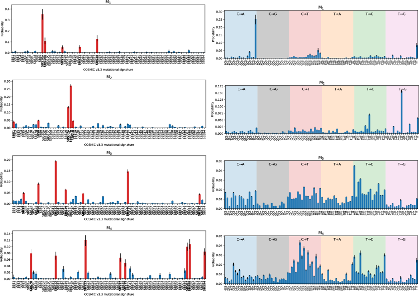
Figure 3: Posterior of four meta-mutational signatures $\phi^{(2)}_{vk}$ (labelled $k=\mathrm{M}_{1},\dots,\mathrm{M}_{4}$) in terms of COSMIC v3.3 mutational signatures $v=\mathrm{SBS}1,\dots,\mathrm{SBS}94$ (left column) and its projection $\sum_{v=\mathrm{SBS}1}^{\mathrm{SBS}94}\phi^{(1)}_{lv}\phi^{(2)}_{vk}$ onto tri-nucleotide single base substitutions $l$ (right column). Bars indicate the average and 95% quantile range of the posterior samples. On the left, mutational signatures exceeding three times the uniform probability have been marked in boldface and red.

Having reviewed the PGBN and introduced our model, we now illustrate its application on small images of handwritten digits and on DNA point mutations in cancer. To evaluate performance, we hold out 50% of the mutations (pixel intensity quanta) from the patients (images) to form a test set, $\mathbf{x}^{\mathrm{test}}$, and evaluate the held-out perplexity as:

$$\mathcal{L}(\mathbf{x}^{\mathrm{test}})=\exp\left(-\frac{1}{J}\sum_{j=1}^{J}\sum_{v=1}^{V}\frac{x_{vj}^{\mathrm{test}}\ln p_{vj}}{x_{{\underline{v}}j}^{\mathrm{test}}}\right),$$ (12)

where $p_{vj}$ is the probability of feature $v$ in example $j$. For non-negative matrix factorisation (NMF) trained on a Kullback-Leibler (KL) loss (which is equivalent to a Poisson likelihood [29]), the probability $p_{vj}=a_{vj}/a_{{\underline{v}}j}$ is the training set reconstruction $a_{vj}\equiv\sum_{k}\phi_{vk}\theta_{kj}$ (so that $a_{vj}\approx x_{vj}$) normalised across features $v$.

Mutatis mutandis, $p_{vj}=\sum_{\sigma=1}^{S}a^{(\sigma)}_{vj}/a^{(\sigma)}_{{\underline{v}}j}$ for the PGBN and MBN where $a_{vj}=\sum_{k=1}^{K_{1}}\phi^{(1)}_{vk}\theta^{(1)}_{kj}$ is the bottom layer activation normalised and averaged over $S$ posterior samples $\sigma=1,\dots,S$ (for the multinomial network $a_{vj}$ is normalised by construction) similar to Refs. [27, 13].

Unlike in [6], for the PGBN we use a gamma distribution to model the scale $c_{j}\sim\operatorname{Gam}(e_{0},f_{0})$ for all layers, instead of a separate beta-distributed $p^{(2)}_{j}$ to set $c_{j}^{(2)}=p^{(2)}_{j}/(1-p^{(2)}_{j})$ for the first layer only. In addition, we consider $\gamma_{0}$ a fixed hyperparameter for both belief networks. For each experiment, four Markov chains were initialised using the prior to ensure overdispersion relative to the posterior (as suggested in Ref. [30]). Each chain was run in parallel on a separate nVidia A40 device.

V-A UCI ML handwritten digits

We considered the UC Irvine Machine Learning Repository dataset [31] (part of Sci-kit learn [32]) containing 1797 images of handwritten digits numbered zero to nine. Each pixel in the eight-by-eight-sized images had a discrete intensity ranging from 0-15 (i.e., four bits) which we modelled as counts. Three separate models with network depth one through three layers ($K_{t}=10$ latent components each layer; hyperparameters $\gamma_{0}=e_{0}=f_{0}=1$, $\eta=0.05$) were run for $10^{5}$ Gibbs burn-in steps and 1280 samples were collected from each chain (thinned to every tenth sample). The hierarchy of topics learned by the network is visualised in Fig. S2, Supplementary Material. The perplexity on holdout pixel intensity quanta were 32.6${}^{+0.1}_{-0.2}$, 32.5${}^{+0.2}_{-0.2}$, and 32.5${}^{+0.1}_{-0.2}$ for one to three layers (lower is better, bootstrapped 95% confidence intervals), respectively. The relatively modest improvement with depth is typical for these models and also observed, e.g., in the PGBN on 20 newsgroup data [6] and below on mutations. For comparison, NMF (from Sci-kit learn [32]) trained using a KL loss achieved a significantly larger (i.e., worse) perplexity of 33.4${}^{+0.2}_{-0.2}$ . In terms of likelihood, all three MBN models converged within 100 iterations of burn-in. Nevertheless, convergence metrics such as $\hat{R}$ [30], comparing between- and within-chain estimates, indicated that the sampler did not fully explore the posterior (not counting the model’s intrinsic symmetries), even after $10^{5}$ burn-in steps. We attributed this to the large number of examples in the dataset. Indeed, running the sampler on a much smaller dataset with only 10 examples leads to satisfactory convergence ($\hat{R}<1.05$ for all latent states on all network configurations after being made permutation symmetry invariant). Furthermore, extensive simulation-based calibration tests [33] for various network configurations on small datasets (we tested up to $J=19$ examples) suggest that our sampler was correctly implemented. The poor mixing is presumably an intrinsic property of our Gibbs sampling approach.

V-B Mutational signature attribution

TABLE I: Perplexity of held-out mutations for inferred mutational signature attributions. Signatures were based on COSMIC v3.3 signature weights. Ninety-five per cent confidence intervals (computed by bootstrapping) are indicated by sub and superscripts. * The perplexity of SigProfilerExtractor was technically infinite due to zero probability being assigned to observed mutations. These samples were removed from the calculations.

Model		Hold out perplexity
SigProfilerExtractor*		64.5${}^{+0.7}_{-0.7}$
Zhou-Cong-Chen	(1 layer)	62.0${}^{+0.7}_{-0.7}$
	(2 layers)	61.9${}^{+0.7}_{-0.7}$
This work	(1 layer)	62.0${}^{+0.7}_{-0.7}$
	(2 layers)	61.9${}^{+0.7}_{-0.7}$

The DNA of cancer cells is peppered with mutations. Instead of uniformly across the genome, mutations occur preferably surrounding specific motifs, leaving a characteristic imprint on the DNA. These imprints are shaped by a combination of mutagenesis, DNA damage sensing, and repair pathways [34]. Mathematically, the mutation spectrum $x_{vj}$, is formed by counting substitutions by three-letter motifs (i.e., tri-nucleotide context, one letter left and right of the substitution, giving 96 features after discounting reverse-complement symmetry). These mutation spectra $x_{vj}$ are canonically decomposed into two non-negative matrices where topics $k$ of $\phi_{vk}$ are called a “mutational signatures” describing how mutations are distributed per signature. Correctly attributing mutations (i.e., solving for $\theta_{kj}$) based on a curated set of weights is becoming increasingly important to guide therapeutic decisions in cancer [35]. The weights $\phi_{vk}^{\mathrm{COSM}}$ from the COSMIC database [36, 37], are the de facto standard in the field, relating spectra across $v=1,\dots,96$ point mutations types to $k=1,\ldots,78$ signatures (named SBS1$,\dots,$SBS94).

V-B1 Performance point mutation dataset

We tested our model on the mutation dataset of Alexandrov et al. [38] comprising approx. 85 million mutations from 4,645 patients. In short, our task is to infer $\theta^{(1)}_{kj}$ given mutation counts $x_{vj}$ and mutational signatures $\phi_{vk}^{\mathrm{COSM}}$. We compared with SigProfilerExtractor, considered the currently most advanced tool for de novo extraction of mutational signatures [39]. Since we expect around five to ten signatures to be present per sample, we set $\gamma_{0}=10$ and other hyperparameters $\eta=e_{0}=f_{0}=1$ for both the Zhou-Cong-Chen and our model and used the greedy layer-wise training procedure (Sec. S4-B, Supplementary Material). Although the test-set likelihood indicated that the chains of both models had not yet fully converged, we halted computation due to the large computation time (a total of 77 and 78 GPU days for MBN and PGBN, respectively). Since the chains were initialised with overdispersed values (compared to the posterior), pre-mature termination of the Markov chains overestimates between-chain variance compared to the “true” posterior. That is, our uncertainty estimates are conservative. Nevertheless, both the Zhou-Cong-Chen and our model more accurately attribute mutations than SigProfilerExtractor (Table I). As expected, both belief networks score comparable with similar architecture.

V-B2 Interpretation meta-signatures

We constructed robust consensus meta-mutational signatures (i.e., topics $\phi_{vk}^{(2)}$ from the second layer) from the MBN (Appendix S4-C) that capture co-occurrence of mutational signatures in patients. This resulted in four meta-signatures denoted $k=\text{M}_{1},\dots,\text{M}_{4}$ (Fig. 3). Summarising meta-signatures by entropy $s(k)=-\sum_{v=1}^{78}\phi^{(2)}_{vk}\ln\phi^{(2)}_{vk}$, we found that the posterior coverage was low with an entropy-based effective sample size [40] of 11, 5, 6, and 6, respectively. We now briefly describe, per meta-signature, the ($K_{1}=78$) mutational signatures, $v$, exceeding three times uniform probability (i.e., $\phi_{vk}^{(2)}\geq 3/K_{1}$, analogous to Ref. [6]).

M₁ describes the co-occurrence of replicative DNA polymerase (POL) $\epsilon$ damage (SBS10a, SBS10b, and SBS28 [41, 42], but not POL $\epsilon$ associated SBS14 [42]) and mismatch-repair deficiency (MMR, SBS15 and SSB21 [43]) (Fig. 3, first row, left column). Tumours with an ultra-hypermutated phenotype (i.e., $\geq$ 100 singlets Mb^-1) typically possess disrupted MMR and POL together [42]. Combined, M₁ describes a preference for altering C$\rightarrow$A and T$\rightarrow$G when flanked by a T on either side (Fig. 3, first row, right column). (Or its complement; we use the pyrimidine base convention like in Ref. [44] by reporting substitutions where the original base was a C or T.).

Meta-signature M₂ primarily captures, presumably, oxidative stress. Its constituents SBS17a/b [45] and SBS18 are thought to be related to DNA oxidation of guanine leading to 8-Oxo-2’-deoxyguanosine (8-oxo-dG) [46, 47, 48, 49]; SBS18 is additionally linked to hydroxyl radicals in culture [50]. Similar to clock-like signature SBS1 (describing spontaneous deamination of 5-methylcytosine [51, 52]), damage due to 8-oxo-dG accumulates in the course of life [53]. To a lesser extent, M₂ also captures SBS8, which is associated with the absence of BRCA{1,2} function in breast cancer [54] and believed to be (uncorrected) replication errors [34]. Characteristically, M₂ prefers T$\rightarrow$G and T$\rightarrow$A singlets with a contextual T on the right-hand side (Fig. 3, second row, right column).

Meta-signature M₃ describes signatures with a strong transcriptional strand bias (SBS5, SBS8, SBS12, SBS16 [38] as well as SBS92 [55] and SBS22 [37]) with the exception of SBS40. Its primary constituent SBS12 is believed to be related to transcription-coupled nucleotide excision repair [38]. The second largest contributor, SBS40, is a spectrally flat, late-replicating [34], signature with spectral similarities to SBS5 (both are related to age [52]) and is believed to be linked to SBS8 [34]. According to COSMIC, some contamination between SBS5 and SBS16 may be present [36, 37]; M₃ is consistent with this observation. Finally, M₃ also captures the co-occurrence with SBS22, which is canonically attributed to aristolochic acid exposure [56, 57, 58]. Overall, M₃ gives rise to a dense spectrum and inherits the quintessential depletion of C substitutions when right-flanked by a G from SBS40 (Fig. 3, third row, right column).

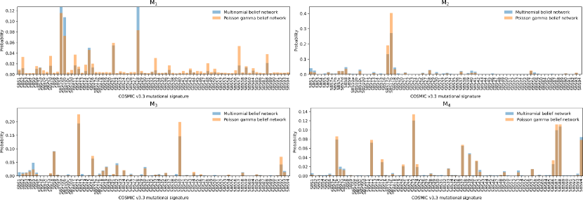
Figure S3: Meta signatures M₁-M₄ replicate in the Poisson gamma believe network (PGBN). The data shows the posterior average of the closest matching meta signatures extracted from the PGBN.

Finally, M₄ describes the co-occurrence of several, seemingly disparate, mutational signatures of known and unknown aetiology. Of known cause are, SBS7b, linked to ultraviolet light (catalysing cyclobutane pyrimidine dimer formation) [58, 59], SBS87 to thiopurine chemotherapy exposure [60] (although its presence has been reported in a thiopurine-naive lung cancer population [61]) and SBS88, related to colibactin-induced damage from the Escherichia coli bacterium [62, 63] (found in mouth cancer [63] and in normal [64] and cancerous [62] colon tissue). Concurrently, M₄ comprises SBS12 [38], SBS23 [52, 54], SBS37 [38], SBS39 [38] and SBS94 [39], all of unknown cause. Jointly, these signatures describe a dense spectrum with a slight tendency for C$\rightarrow$T substitutions. Reassuringly, meta-signatures M${}_{1},\dots,$M₄ replicated independently in the PGBN (Fig. S3, Supplementary Material). To our knowledge, this is the first time a first-principles characterisation of the organising principles of mutagenic processes in cancer has been carried out.

VI Discussion & Conclusion

In this paper, a deeper (i.e., multi-layer) extension of latent Dirichlet allocation was proposed that mirrors the Zhou-Cong-Chen model [6]. The principal difference with Ref. [6] is that the observed data are multinomial instead of Poisson distributed. That is, the total number of observations per example is considered fixed (i.e., conditioned on). Furthermore, the model’s weights are constrained to lie within the simplex (by virtue of the Dirichlet distribution) whilst the dispersion of each layer is controlled by a single parameter similar to the hierarchical Dirichlet process [10] to allow sharing of statistical strength between samples. The hierarchical setup allows the model to discover increasingly abstract representations of the data. As a case in point, we applied our model to mutations in cancer in which we discovered four meta-signatures describing the co-occurrence of mutagenic processes in cancer. To our knowledge, this is the first time such a first-principles characterisation of mutagenic processes in cancer has been described. Furthermore, our Bayesian approach is inherently robust against overfitting which is useful when the data is sparse or data collection is expensive. Both aspects are commonly encountered in healthcare data. Other contributions of this paper are the relation between the Dirichlet-multinomial distribution, the Chinese restaurant table distribution, and the Polya urn scheme which to the best of our knowledge is novel, and a comprehensive review of the Zhou-Cong-Chen model.

Scaling up to large datasets remains challenging using our Gibbs sampling approach, despite our GPU implementation that can run on multiple accelerators using JAX [65]. Approximate Markov chain Monte Carlo [20] and hybrid approaches [22, 23] are an attractive middle-ground between exact and approximate inference that can scale deep probabilistic models to large datasets. We leave this challenging problem for future work.

Hylke Donker is postdoctoral researcher at University Medical Center Groningen at Groningen, Groningen, 9700 RB, the Netherlands. His research interests include machine learning and applications in medicine. Donker received his PhD in quantum physics from Radboud University, the Netherlands. Contact him at h.c.donker@umcg.nl.

Dorien Neijzen is a PhD candidate at University Medical Center Groningen at Groningen, Groningen, 9700 RB, the Netherlands. Her research interests include (Bayesian) statistics, unsupervised machine learning, and applications in medicine and neuroscience. Neijzen received her MSc in theoretical physics from University of Amsterdam, the Netherlands. Contact her at d.neijzen@umcg.nl.

Gerton Lunter is Professor of Medical Statistics at University Medical Center Groningen, the Netherlands. His research interests include Bayesian statistics and machine learning, and their application to functional genomics, statistical genetics and population cohort data. After receiving his PhD in Mathematics from the University of Groningen, he worked at Philips Research Eindhoven before moving to Oxford, UK where he worked in various roles at the department of Statistics, the Wellcome Trust Centre for Human Genetics, and the Weatherall Institute of Molecular Medicine.

S1 Preliminaries

A sampling strategy for a Bayesian network involves a series of marginalization and augmentation steps, with relations between distributions that can be summarized by factorizations such as

$$p(x)p(y|x)=p(y)p(x|y),$$ (S1)

which implies $p(x)=\int p(y)p(x|y)\mathrm{d}y$, a relation that can be used either to marginalize $y$ or to augment with $y$. The first factorization we use involves the Poisson distribution. Let

$$x_{j}\sim\operatorname{Pois}(\lambda_{j});\qquad y=x_{\underline{j}},$$ (S2)

where underlined indices denote summation, $x_{\underline{j}}:=\sum_{j}x_{j}$, and we write vectors as $\{x_{j}\}_{j}$, dropping the outer index $j$ when there is no ambiguity. Then $y$ is also Poisson distributed, and conditional on $y$ the $x_{j}$ have a multinomial distribution:

$$y\sim\operatorname{Pois}(\lambda_{\underline{j}});\qquad\{x_{j}\}\sim\operatorname{Mult}(y,\{\lambda_{j}/\lambda_{\underline{j}}\}).$$ (S3)

This is an instance of (S1) if the deterministic relationship $y=x_{\underline{j}}$ is interpreted as the degenerate distribution $p(y|\{x_{j}\})=\delta_{x_{\underline{j}},y}$. Distributions hold conditional on fixed values of variables that appear on the right-hand side; for instance the distribution of $\{x_{j}\}$ in (S3) is conditional on both $\{\lambda_{j}\}$ and $y$, while in (S2) $x_{j}$ is conditioned on $\lambda_{j}$ only.

The negative binomial distribution can be seen as an overdispersed version of the Poisson distribution, in two ways. First, we can write it as a gamma-Poisson mixture. The joint distribution defined by

$$\lambda\sim\operatorname{Gam}(a,c);\qquad x\sim\operatorname{Pois}(q\lambda),$$ (S4)

is the same as the joint distribution defined by

$$x\sim\operatorname{NB}(a,{q\over q+c});\qquad\lambda\sim\operatorname{Gam}(a+x,c+q),$$ (S5)

also showing that the gamma distribution is a conjugate prior for the Poisson distribution. Note that we use the shape-and-rate parameterization of the gamma distribution.

The negative binomial can also be written as a Poisson-Logarithmic mixture [1]. Let $\operatorname{Log}(p)$ be the distribution with probability mass function

$$\operatorname{Log}(k;p)={-1\over\ln(1-p)}{p^{k}\over k},$$

where $0<p<1$, and define $n\sim\operatorname{SumLog}(l,p)$ by $u_{i}\sim\operatorname{Log}(p)$ for $i=1,\ldots,l$, and $n=\sum_{i=1}^{l}u_{i}$. Then, the joint distribution over $l$ and $n$ defined by

$$n\sim\operatorname{NB}(a,p);\qquad l\sim\operatorname{CRT}(n,a),$$ (S6)

is the same as

$$l\sim\operatorname{Pois}(-a\ln(1-p));\qquad n\sim\operatorname{SumLog}(l,p),$$ (S7)

where $\operatorname{CRT}$ is the Chinese restaurant table distribution [2]. This factorization allows augmenting a gamma-Poisson mixture (the negative binomial $n$) with a pure Poisson variate $l$, which is a crucial step in the deep Poisson factor analysis model. For an extension of the model we will need a similar augmentation of a Dirichlet-multinomial mixture with a pure multinomial. It can be shown (see S1-A below) that the joint distribution over $\{x_{k}\}$ and $\{y_{k}\}$ defined by

$$\{x_{k}\}\sim\operatorname{DirMult}(n,\{\lambda_{k}\});\qquad y_{k}\sim\operatorname{CRT}(x_{k},\lambda_{k});\qquad m=y_{\underline{k}}$$ (S8)

is the same as the joint distribution over $\{x_{k}\}$ and $\{y_{k}\}$ defined by

$$m\sim\operatorname{CRT}(n,\lambda_{\underline{k}});\qquad\{y_{k}\}\sim\operatorname{Mult}(m,\{\lambda_{k}\});\qquad\{x_{k}\}\sim\operatorname{Polya}(n,\{y_{k}\}),$$ (S9)

Here $\operatorname{Polya}(n,\{y_{k}\})$ is the distribution of the contents of an urn after running a Polya scheme (drawing a ball, returning the drawn ball and a new identically colored one each time, until the urn contains $n$ balls), where the urn initially contains $y_{k}$ balls of color $k$. It is straightforward to see that $\operatorname{Polya}(n,\{y_{k}\})=\{y_{k}\}+\operatorname{DirMult}(n-m,\{y_{k}\}$).

S1-A Proof of Dirichlet-multinomial-CRT factorization (Theorem 1; eqs. (S8)-(S9))

A draw from a Dirchlet-multinomial is defined by

$$\{p_{j}\}\sim\operatorname{Dir}(\{\lambda_{j}\});\qquad\{x_{j}\}\sim\operatorname{Mult}(n,\{p_{j}\});\qquad\{x_{j}\}\sim\operatorname{DirMult}(n,\{\lambda_{j}\})$$

By building up a draw from the multinomial as $n$ draws from a categorical distribution and using Dirichlet-multinomial conjugacy we get the Polya urn scheme,

$$\{x^{(1)}_{j}\}\sim\operatorname{Mult}(1,\{\lambda_{j}\});\qquad\{x^{(i+1)}_{j}\}\sim\{x^{(i)}_{j}\}+\operatorname{Mult}(1,\{\lambda_{j}+x^{(i)}_{j}\}),$$

where $x_{j}=x_{j}^{(n)}$ and to simplify notation we dropped the normalization of the multinomial’s probability parameter. This scheme highlights the overdispersed or ”rich get richer” character of the Dirichlet-multinomial mixture distribution.

For the proof of (S8)-(S9), recall that a draw from the Chinese Restaurant Table distribution $t\sim\operatorname{CRT}(n,\lambda)$ is generated by a similar scheme. Starting with an urn containing a single special ball with weight $\lambda$, balls are drawn $n$ times, and each time the drawn ball is returned together with a new, ordinary ball of weight $1$. The outcome $t$ is the number of times the special ball was drawn.

Now return to the Polya urn scheme above and let the initial $j$-colored balls of weight $\lambda_{j}$ be made of iron, let $j$-colored balls that are added because an iron $j$-colored ball was drawn be made of oak, and let other balls be made of pine. Wooden balls have weight $1$ and all balls are drawn with probability proportional to their weight. Let $x_{j}$ be the final number of $j$-colored wooden balls in the urn, let $y_{j}$ be the final number of $j$-colored oak balls, and $m$ the final number of oak balls of any color.

Using the equivalence between the Polya urn scheme and the Dirichlet multinomial we see that $\{x_{k}\}$ follow a Dirichlet multinomial distribution with parameters $n$ and $\{\lambda_{j}\}$. By focusing on material and ignoring color, we see that $m$ follows a CRT distribution with parameters $n$ and $\lambda_{\underline{j}}$. Similarly, focusing only on $j$-colored balls shows that conditional on $x_{j}$, $y_{j}$ again follows a CRT distribution, with parameters $x_{j}$ and $\lambda_{j}$, since the only events of interests are drawing a $j$-colored iron or wooden ball, which have probabilities proportional to $\lambda_{j}$ and $1$ respectively. Since iron balls are drawn with probability proportional to their weight, conditional on $m$ the distribution over colors among the $m$ oak balls is multinomial with parameters $m$ and $\{\lambda_{j}\}$. Finally, conditional on knowing the number and color of the oak balls $\{y_{j}\}$, the process of inserting the remaining pine balls is still a Polya process except that events involving drawing iron balls are now forbidden, so that the distribution of pine balls $\{x_{j}-y_{j}\}$ is again a Dirichlet-multinomial but with parameters $n-m$ and $\{y_{j}\}$. This proves (S8) and (S9).

S1-B Sampling the concentration parameters of a Dirichlet distribution

In models similar to the one considered here, the concentration parameters of a Dirichlet distribution are often kept fixed [3, 4, 5] or inferred by maximum likelihood [6]. The factorization above makes it possible to efficiently generate posterior samples from the concentration parameters, under an appropriate prior and given multinomial observations driven by draws from the Dirichlet. The setup is

$$\alpha \sim\operatorname{Gam}(a,b);\quad\{\eta_{k}\}\sim\operatorname{Dir}(\{\eta^{0}_{k}\});\quad$$

$$\{x_{jk}\}_{k} \sim\operatorname{DirMult}(n_{j},\{\alpha\eta_{k}\}_{k});\quad y_{jk}\sim\operatorname{CRT}(x_{jk},\alpha\eta_{k});\quad m_{j}=y_{j{\underline{k}}}.$$ (S10)

where we have written the concentration parameters as the product of a probability vector $\{\eta_{k}\}$ and a scalar $\alpha$; these will be given Dirichlet and Gamma priors respectively. By the factorization above this is the same joint distribution as

$$\alpha \sim\operatorname{Gam}(a,b);\quad\{\eta_{k}\}\sim\operatorname{Dir}(\{\eta^{0}_{k}\});\quad$$

$$m_{j} \sim\operatorname{CRT}(n_{j},\alpha);\quad\{y_{jk}\}_{k}\sim\operatorname{Mult}(m_{j},\{\eta_{k}\});\quad\{x_{jk}\}_{k}\sim\operatorname{Polya}(n_{j},\{y_{jk}\}_{k}).$$ (S11)

The numbers $m_{j}$ represent the total number of distinct groups in a draw from a Dirichlet process, given the concentration parameter $\alpha$ [7]. Evidence for the value of $\alpha$ is encoded in the (unobserved) $m_{j}$, which in turn are determined by the (unobserved) $y_{jk}$ which sort the unobserved groups into $K$ separate subgroups conditional on the observed counts $x_{jk}$. The likelihood of the number of distinct groups $m$ in a draw from a Dirichlet process given the concentration parameter $\alpha$ and total number of draws $n$ is given by the probability mass function of the CRT distribution,

$$p(m|\alpha,n)=s(n,m)\alpha^{m}{\Gamma(\alpha)\over\Gamma(\alpha+n)},$$ (S12)

where $s(n,m)$ are unsigned Stirling numbers of the first kind [2, 7]. By multiplying over observations $j$ a similar likelihood is obtained for multiple observations, together with a gamma prior on $\alpha$ results in a posterior distribution that we refer to as the CRT-gamma posterior:

$$\alpha\sim\operatorname{Gam}(a,b);\quad m_{j}\sim\operatorname{CRT}(n_{j},\alpha);\quad\alpha\sim\operatorname{CRTCP}(m_{\underline{j}},\{n_{j}\}_{j},a,b),$$ (S13)

where $\operatorname{CRTCP}(\alpha|m,\{n_{j}\}_{j},a,b)\propto\operatorname{Gam}(\alpha|a,b)\alpha^{m}\prod_{j}\frac{\Gamma(\alpha)}{\Gamma(\alpha+n_{j})}$ [7]. A sampling scheme for $\alpha$ for the likelihood (S12) and a Gamma prior was devised by [8], and was extended by [7] to the case of multiple observations (S13). Finally, the multinomial distribution of $\{y_{jk}\}_{k}$ is conjugate to the Dirichlet prior on $\{\eta_{k}\}$ leading to

$$\{\eta_{k}\}\sim\operatorname{Dir}(\{\eta^{0}_{k}\});\qquad\{y_{jk}\}_{k}\sim\operatorname{Mult}(m_{j},\{\eta_{k}\}_{k});\qquad\{\eta_{k}\}\sim\operatorname{Dir}(\{\eta^{0}_{k}+y_{{\underline{j}}k}\}).$$ (S14)

S1-C Sampling parameters of the gamma distribution

If a Poisson-distributed observation with rate proportional to a gamma-distributed variable is available, we can use conditional conjugacy to sample the posterior of the gamma parameters. Suppose that

$$\alpha\sim\operatorname{Gam}(a_{0},b_{0});\quad\beta\sim\operatorname{Gam}(e_{0},f_{0});\quad\theta\sim\operatorname{Gam}(\alpha,\beta);\quad m\sim\operatorname{Pois}(q\theta),$$

and that $\theta$ is not observed, but the count $m$ is. Marginalizing $\theta$ we get $m\sim\operatorname{NB}(\alpha,q/(q+\beta))$. Augmenting with $x\sim\operatorname{CRT}(m,\alpha)$ and using (S6) and (S7) we find that $x\sim\operatorname{Pois}[\alpha\ln(1+q/\beta)]$. Using gamma-Poisson conjugacy gives the mutually dependent update equations

$$x\sim\operatorname{CRT}(m,\alpha);\quad\alpha\sim\operatorname{Gam}(a_{0}+x,b_{0}+\ln{(1+q/\beta)}).$$ (S15)

As posterior for $\theta$ given $m$ we get $\theta\sim\operatorname{Gam}(\alpha+m,\beta+q)$; augmenting with $\theta$ and using the gamma-gamma conjugacy

$$\beta\sim\operatorname{Gam}(e_{0},f_{0});\qquad\theta\sim\operatorname{Gam}(\alpha,\beta);\qquad\beta\sim\operatorname{Gam}(e_{0}+\alpha,f_{0}+\theta).$$ (S16)

results in the mutually dependent update equations

$$\theta\sim\operatorname{Gam}(\alpha+m,\beta+q);\quad\beta\sim\operatorname{Gam}(e_{0}+\alpha,f_{0}+\theta).$$ (S17)

S2 Gamma belief network

Since many of the techniques of the Gamma belief network of Zhou et al. [5] apply to the multinomial belief network, we start by summarising and reviewing their method in some detail. We stay close to their notation, but have made some modifications where this simplifies the future connection to the multinomial belief network.

S2-A Backbone of feature activations

The backbone of the model is a stack of Gamma-distributed hidden units $\theta^{(t)}_{vj}$, with the last one parameterizing a Poisson distribution generating observed counts $x_{vj}$, one for each sample $j$ and feature $v$. The generative model is

$$a_{vj}^{(T+1)} =r_{v},$$ (S18)

$$\theta^{(t)}_{vj} \sim\operatorname{Gam}(a_{vj}^{(t+1)},{c_{j}^{(t+1)}}), t=T,\ldots,1$$ (S19)

$$a_{vj}^{(t)} =\sum_{k=1}^{K_{t}}\phi^{(t)}_{vk}\theta^{(t)}_{kj}, t=T,\ldots,1$$ (S20)

$$x_{vj} \sim\operatorname{Pois}(a_{vj}^{(1)}).$$ (S21)

For $T=1$ we only have one layer, and the model reduces to $x_{vj}=\operatorname{Pois}([\boldsymbol{\phi\theta}]_{vj})$, called Poisson Factor Analysis [4]. For multiple layers, the features $\boldsymbol{\theta}^{(t+1)}$ on layer $t+1$ determine the shape parameters of the gamma distributions on layer $t$ through a connection weight matrix $\boldsymbol{\phi}^{(t+1)}\in\mathbb{R}^{K_{t}\times K_{t+1}}$, so that $\boldsymbol{\phi}^{(t+1)}$ induces correlations between features on level $t$. The lowest-level activations $\boldsymbol{a}^{(1)}$ are used to parameterize a Poisson distribution, which generates the observed count variables $x_{vj}$ for individual (document, observation) $j$. Below we will treat $r_{v}$ and $c_{j}^{(t)}$ as random variables and targets for inference, but for now, we consider them as fixed parameters and focus on inference of $\boldsymbol{\phi}^{(t)}$ and $\boldsymbol{\theta}^{(t)}_{j}$. We will assume that $\sum_{v}\phi^{(t)}_{vk}=1$, which later on is enforced by Dirichlet priors on $\boldsymbol{\phi}_{k}$.

This model architecture is similar to a $T$-layer neural network, with $\boldsymbol{a}^{(t)}$ playing the role of activations that represent the activity of features (topics, factors) of increasing complexity as $t$ increases. In the remainder, we use the language of topic models, so that $x_{vj}$ is the number of times word $v$ is used in document $j$, and $\phi^{(1)}_{vk}$ is the probability that word $v$ occurs in topic $k$. This is for the lowest level $1$; we will similarly refer to level-$t$ topics and level-$t$ “words”, the latter representing the activity of corresponding topics on level $t-1$.

Different from [5] we use a Gamma-distributed variate $c_{j}^{(2)}$ as rate parameter of the gamma distribution for $\theta^{(1)}$, instead of $p_{j}^{(2)}/1-p_{j}^{(2)}$ where $p_{j}^{(2)}$ has a Beta distribution; we will come back to this choice below.

S2-B Augmentation with latent counts

We review Zhou’s augmentation and marginalization scheme that enables efficient inference for this model. First, introduce new variables

$$x^{(t)}_{vj}\sim\operatorname{Pois}(q_{j}^{(t)}a^{(t)}_{vj}),\qquad t=1,\ldots,T+1$$ (S22)

where we set $q_{j}^{(1)}=1$ so that we can identify $x^{(1)}_{vj}$ with the observed counts $x_{vj}$; the $q_{j}^{(t)}$ for $t>1$ will be defined below. Using (S2)-(S3) we can augment $x^{(t)}_{vj}$ as

$$y^{(t)}_{vjk} \sim\operatorname{Pois}(q^{(t)}_{j}\phi^{(t)}_{vk}\theta^{(t)}_{kj});$$ (S23)

$$x^{(t)}_{vj} =y^{(t)}_{vj\underline{k}}.$$ (S24)

The counts $y_{vjk}^{(t)}$ represent a possible assignment of level-$t$ words to level-$t$ topics. Marginalizing over $v$ and using (S2)-(S3) again we get the augmentation

$$m_{jk}^{(t)} :=y_{\underline{v}jk}^{(t)}\sim\operatorname{Pois}(q_{j}^{(t)}\theta^{(t)}_{kj});$$ (S25)

$$y_{vjk} =\operatorname{Mult}(m^{(t)}_{jk},\{\phi^{(t)}_{vk}\}_{v}).$$ (S26)

since $\phi^{(t)}_{\underline{v}k}=1$. These counts represent level-$t$ topic usage in document $j$. Now, marginalizing $\boldsymbol{\theta}^{(t)}$ turns $m_{jk}^{(t)}$ into an overdispersed Poisson distribution; from (S19) we see that $\boldsymbol{\theta}^{(t)}$ is Gamma distributed, so it becomes a negative binomial:

$$m_{jk}^{(t)} \sim\operatorname{NB}(a^{(t+1)}_{kj},q^{(t)}_{j}/(q^{(t)}_{j}+c^{(t+1)}_{j})),$$ (S27)

using (S4) and (S5). This gives us a count variable that is parameterized by the activation of the layer above $t$, but one which follows a negative binomial distribution rather than a Poisson distribution (S22). However, using (S6) and (S7) we can augment once more to write the negative binomial as a Poisson-Logarithmic mixture:

$$x_{kj}^{(t+1)}\sim\operatorname{Pois}(a_{kj}^{(t+1)}\ln{q^{(t)}_{j}+c_{j}^{(t+1)}\over c_{j}^{(t+1)}});\qquad m_{jk}^{(t)}\sim\operatorname{SumLog}(x_{kj}^{(t+1)},{q^{(t)}_{j}\over q^{(t)}_{j}+c_{j}^{(t+1)}}),$$ (S28)

so that $x^{(t+1)}_{kj}$ agrees with (S22) if we choose

$$q_{j}^{(t+1)}:=\ln{q_{j}^{(t)}+c_{j}^{(t+1)}\over c_{j}^{(t+1)}}.$$ (S29)

This allows us to continue the procedure for layer $y+1$, and so on until $t=T$, sampling augmented variables $y^{(t)}_{vjk}$, $m^{(t)}_{jk}$ and $x^{(t+1)}_{kj}$ for $t=1,\ldots,T$.

S2-C Alternative representation as Deep Poisson Factor model

The procedure described in section S2-B not only augments the model with new counts but also integrates out $\boldsymbol{\theta}^{(t)}$. This provides an alternative and equivalent representation as a generative model. Starting from $a^{(t+1)}_{kj}$ we can use (S28), (S26) and (S24) to sample $x^{(t+1)}_{kj}$, $m^{(t)}_{jk}$, $y_{vjk}^{(t)}$, and finally $x_{vj}^{(t)}$. Continuing downwards this shows how to eventually generate the observed counts $x^{(1)}_{vj}$ using count variables, while $\boldsymbol{\theta}^{(t)}$ is integrated out. Explicitly, the generative model becomes

$$x_{kj}^{(t+1)}\sim\operatorname{Pois}(q_{j}^{(t+1)}a_{kj}^{(t+1)});$$

$$m_{jk}^{(t)}\sim\operatorname{SumLog}(x_{kj}^{(t+1)},1-e^{-q_{j}^{(t+1)}});\qquad\{y_{vjk}^{(t)}\}_{v}\sim\operatorname{Mult}(m_{jk}^{(t)},\{\phi_{vk}^{(t)}\}_{v});\qquad x_{vj}^{(t)}:=y_{vj{\underline{k}}}^{(t)}.$$

(Note that throughout we condition on $q^{(t)}_{j}$ for all $t$, and therefore on all $c_{j}^{(t)}$ as well; we also haven’t specified how to sample $\phi^{(t)}_{vk}$ yet.) This equivalent generative process motivates the name Deep Poisson Factor Analysis. The two alternative schemes are shown graphically in figure S1.

Figure S1: Two equivalent generative models for a count variable $\boldsymbol{x}^{(1)}$ from the Poisson gamma believe network, using (a) a tower of real-valued latent variables $\boldsymbol{\theta}$, $\boldsymbol{a}$, or (b) latent counts $\boldsymbol{m}$, $\boldsymbol{y}$, $\boldsymbol{x}$. Blunt arrows indicate deterministic relationships. The variable $\boldsymbol{q}^{(1)}$ is a dummy and has a fixed value $1$. The counts $\boldsymbol{x}^{(t)}$ and variables $\boldsymbol{q}^{(t)}$, $t>1$, in the left representation, are included for clarity (and have the same distribution as the variables in the right model) but are not used to generate the outcome $\boldsymbol{x}^{(1)}$, and so can be marginalized out.

S2-D Sampling per-document latent variables

The derivation above can be used to sample the latent counts conditional on observations (and parameters $\boldsymbol{\phi}$, $\boldsymbol{\theta}$ and $\boldsymbol{r}$), from layer 1 upwards. These steps are,

$$y_{vjk}^{(t)} \sim\operatorname{Mult}(x^{(t)}_{vj},\{\phi^{(t)}_{vk}\theta_{kj}^{(t)}\}_{k});$$ (S30)

$$m^{(t)}_{jk} =y^{(t)}_{{\underline{v}}jk};$$ (S31)

$$x_{kj}^{(t+1)} \sim\operatorname{CRT}(m_{jk}^{(t)},a_{kj}^{(t+1)}),$$ (S32)

where for (S30) we used (S2)-(S3) and (S23)-(S24); and for (S32) we used (S6)-(S7) and (S27)-(S28). Note that after the last step $x_{kj}^{(t+1)}$ is no longer conditioned on $\theta^{(t)}_{kj}$ because it is integrated out, however, explicit values for $\theta^{(t)}_{kj}$ are used in (S30). To sample new values for $\theta^{(t)}_{kj}$, we use Gamma-Poisson conjugacy (S4)-(S5) on (S19) and (S25) to get

$$\theta^{(t)}_{kj}\sim\operatorname{Gam}(a^{(t+1)}_{kj}+m^{(t)}_{kj},c^{(t+1)}_{j}+q_{j}^{(t)}).$$ (S33)

In order to sample the final set of per-document variables, the inverse scaling parameters $c_{j}^{(t)}$, we first need to integrate out $q_{j}^{(t)}$ since it depends on $c_{j}^{(t)}$ via (S29). That means we also need to integrate out $x_{vj}^{(t)}$ and $m^{(t-1)}_{jk}$ which both depend on $q_{j}^{(t)}$, as well as $y^{(t-1)}_{vjk}$ because of the deterministic relationship (S25). We do not need to marginalize other variables as $\boldsymbol{x}^{(t-1)}$ and its dependents are conditionally independent of $\boldsymbol{x}^{(t)}$ given $\boldsymbol{\theta}^{(t-1)}$, as can be seen from figure 2a. Once $\boldsymbol{x}^{(t)}$, $\boldsymbol{m}^{(t-1)}$ and $\boldsymbol{y}^{(t-1)}$ are integrated out, $\theta_{vj}^{(t-1)}$ is related to $c_{j}^{(t)}$ solely through (S19), and marginalizing this over $v$ we get

$$\theta^{(t-1)}_{{\underline{v}}j}\sim\operatorname{Gam}(a^{(t)}_{{\underline{v}}j},c_{j}^{(t)}),\qquad(t=2,\ldots,T+1).$$

where $a^{(t)}_{{\underline{v}}j}=\theta_{{\underline{k}}j}^{(t)}$ for $t=2,\ldots,T$, and $a^{(T+1)}_{{\underline{v}}j}=r_{{\underline{v}}}$. The conjugate prior for a gamma likelihood with fixed shape parameter is a gamma distribution again. This gives the following prior and posterior distributions for $c_{j}^{(t)}$:

$$c_{j}^{(t)}\sim\operatorname{Gam}(e_{0},f_{0});\qquad c_{j}^{(t)}\sim\operatorname{Gam}(e_{0}+a^{(t)}_{{\underline{v}}j},f_{0}+\theta^{(t-1)}_{{\underline{k}}j}).\qquad(t=2,\ldots,T+1)$$ (S34)

As an aside, note that it is possible to integrate out $\boldsymbol{\phi}^{(1)}$ and $\boldsymbol{\theta}^{(1)}$, in the same way as is done in the collapsed Gibbs sampler for the LDA model. This is done in [5] and may lead to faster mixing. However, if we do that no $\boldsymbol{\theta}^{(1)}$ is available to construct a posterior for $\boldsymbol{c}^{(2)}$ as in (S34). Instead, (S27) can be used:

$$m_{jk}^{(1)}\sim\operatorname{NB}(a^{(2)}_{kj},1/(1+c_{j}^{(2)})),$$

using that $q_{j}^{(1)}=1$. Using the beta-negative binomial conjugacy, we can write

$$p^{(2)}\sim\operatorname{Beta}(a_{0},b_{0});\qquad p^{(2)}\sim\operatorname{Beta}(a_{0}+a^{(2)}_{{\underline{k}}j},b_{0}+m_{j{\underline{k}}}^{(1)}),$$

where we defined

$$p^{(2)}:=(1+c_{j}^{(2)})^{-1},\qquad\text{so that}\qquad c_{j}^{(2)}=(1-p^{(2)})/p^{(2)},$$

which gives $\boldsymbol{c}^{(2)}$ a Beta distribution of the second kind. We cannot similarly integrate out $\boldsymbol{\theta}^{(t)}$ and $\boldsymbol{\phi}^{(t)}$ for $t>1$ as already for collapsed Gibbs sampling, values for $\boldsymbol{\theta}^{(2)}$ and $\boldsymbol{\phi}^{(2)}$ are necessary to define the prior on $\boldsymbol{\theta}^{(1)}$.

S2-E Sampling $\boldsymbol{\phi}$ and $\boldsymbol{r}$

It remains to sample the model-level parameters $\phi^{(t)}_{vk}$, $\eta^{(t)}_{v}$, and $r_{v}$. For $\boldsymbol{\phi}$ we marginalize (S26) over $j$ and, noting that the multinomial is conjugate to a Dirichlet, we use a Dirichlet prior for $\boldsymbol{\phi}$ to obtain the update equations

$$\{\phi^{(t)}_{vk}\}_{v}\sim\operatorname{Dir}(\{\eta^{(t)}_{v}\}_{v});\qquad\{y_{v{\underline{j}}k}^{(t)}\}_{v}\sim\operatorname{Mult}(m_{{\underline{j}}k}^{(t)},\{\phi^{(t)}_{vk}\}_{v});\qquad\{\phi^{(t)}_{vk}\}_{v}\sim\operatorname{Dir}(\{\eta^{(t)}_{v}+y^{(t)}_{v{\underline{j}}k}\}_{v}).$$ (S35)

To sample $\{\eta^{(t)}_{v}\}$, we integrate out $\phi^{(t)}_{vk}$ and consider $x_{v{\underline{j}}k}^{(t)}$ as a draw from a Dirichlet-multinomial distribution with parameters $\alpha^{(t)}\eta_{v}^{(t)}$ where the factors $\alpha^{(t)}$ and $\{\eta_{v}^{(t)}\}$ have Gamma and Dirichlet priors respectively, as in (S10). This results in the following update equations,

$$\alpha^{(t)} \sim\operatorname{Gam}(a,b);\quad\{\eta^{(t)}_{v}\}_{v}\sim\operatorname{Dir}(\{\eta_{v,0}\}_{v});\quad\{y^{(t)}_{v{\underline{j}}k}\}_{v}\sim\operatorname{DirMult}(m_{{\underline{j}}k}^{(t)},\{\alpha^{(t)}\eta_{v}^{t}\}_{v});\quad$$

$$z^{(t)}_{vk} \sim\operatorname{CRT}(y^{(t)}_{v{\underline{j}}k},\alpha^{(t)}\eta^{(t)}_{v});\quad\alpha\sim\operatorname{CRTCP}(z^{(t)}_{{\underline{v}}{\underline{k}}},\{m_{{\underline{j}}k}^{(t)}\}_{k},a,b);\quad\{\eta^{(t)}_{v}\}_{v}\sim\operatorname{Dir}(\{\eta_{v,0}+z^{(t)}_{v{\underline{k}}}\}_{v}).$$ (S36)

For $r_{v}$ we use (S28) and (S29) for $t=T$, marginalize $j$, and use gamma-Poisson conjugacy to get update equations

$$r_{v}\sim\operatorname{Gam}(\gamma_{0}/K_{T},c_{0});\qquad x^{(T+1)}_{v{\underline{j}}}\sim\operatorname{Pois}(r_{v}q_{{\underline{j}}}^{(T+1)});\qquad r_{v}\sim\operatorname{Gam}(\gamma_{0}/K_{T}+x^{(T+1)}_{v{\underline{j}}},c_{0}+q_{{\underline{j}}}^{(T+1)})$$ (S37)

S2-F Sampling strategy

It is helpful to think of the model as organised as an alternating stack of layers, one taking inputs $\boldsymbol{a}$ and $\boldsymbol{c}$ and using the gamma distribution to produce an output $\boldsymbol{\theta}$; and one taking $\boldsymbol{\theta}$ and edge weights $\boldsymbol{\phi}$ to produce an activation $\boldsymbol{a}$. During inference, the model also uses latent variables $x_{vj}$, $y_{vjk}$, $m_{jk}$ and $q_{j}$. Inference proceeds in two main stages. First, the $\boldsymbol{q}^{(t)}$ are calculated, followed by augmentation with the $\boldsymbol{y}$, $\boldsymbol{m}$ and $\boldsymbol{x}^{(t)}$ $(t\geq 2)$ count variables going up the stack, while marginalising $\boldsymbol{\phi}$, and also updating the $\boldsymbol{\phi}$ variables. After updating the parameter $\boldsymbol{r}$, the second stage involves updating $\boldsymbol{c}$ and $\boldsymbol{\theta}$ going down the stack, while the augmented count variables are dropped again. Table S1 provides a detailed overview.

			factor-layer $1$								factor-layer $2$
								gamma layer $1$								gamma layer $2$
Stage	Eq.	(Eq.)	$x^{1}$	$q^{1}$	$a^{1}$	$\phi^{1}$	$y^{1}$	$\theta^{1}$	$m^{1}$	$c^{2}$	$x^{2}$	$q^{2}$	$a^{2}$	$\phi^{2}$	$y^{2}$	$\theta^{2}$	$m^{2}$	$c^{3}$	$x^{3}$	$q^{3}$	$r$
			O	1	x	x	-	x	-	x	-	-	x	x	-	x	-	x	-	-	x
0 (all $t$)	(S29)	(S55)	O	1x	x	x	-	x	-	x	-	U	x	x	-	x	-	x	-	U	x
1 ($t$=1)	(S30)	(S52)	O	1	x	x	S	x	-x	x	-	x	x	x	-	x	-	x	-	x	x
2 ($t$=1)	(S35)	(S35)	O	1	-x	S	x	x	-	x	-	x	x	x	-	x	-	x	-	x	x
3 ($t$=1)	(S31)	(S53)	O	1	-	x	x	x	U	x	-	x	x	x	-	x	-	x	-	x	x
4 ($t$=1)	(S32)	(S54)	O	1	-	x	x	-x	x	x	S	x	x	x	-x	x	-	x	-	x	x
1 ($t$=2)	(S30)	(S52)	O	1	-	x	x	-	x	x	x	x	x	x	S	x	-x	x	-	x	x
2 ($t$=2)	(S35)	(S35)	O	1	-	x	x	-	x	x	x	x	-x	S	x	x	-	x	-	x	x
3 ($t$=2)	(S31)	(S53)	O	1	-	x	x	-	x	x	x	x	-	x	x	x	U	x	-	x	x
4 ($t$=2)	(S32)	(S54)	O	1	-	x	x	-	x	x	x	x	-	x	x	-x	x	x	S	x	x
r	(S37)	(S58)	O	1	-	x	x	-	x	x	x	x	-	x	x	-	x	x	x	x	S
5 ($t$=2)	(S33)	(S56)	O	1	-	x	x	-	x	x	x	x	-x	x	x	S	x	x	x	x	x
6 ($t$=2)	(S34)	(S57)	O	1	-	x	x	-	x	x	x	x	-	x	-x	x	-x	S	-x	-x	x
7 ($t$=2)	(S20)	(S40)	O	1	-	x	x	-	x	x	x	x	U	x	-	x	-	x	-	-	x
5 ($t$=1)	(S33)	(S56)	O	1x	-x	x	x	S	x	x	x	x	x	x	-	x	-	x	-	-	x
6 ($t$=1)	(S34)	(S57)	O	1	-	x	-x	x	-x	S	-x	-x	x	x	-x	x	-x	x	-x	-x	x
7 ($t$=1)	(S20)	(S40)	O	1	U	x	-	x	-	x	-	-	x	x	-	x	-	x	-	-	x

TABLE S1: Variable instantiation and marginalisation during inference. Upper indices denote layer number (without parentheses). Lower indices are suppressed. All variables include the observation index $j$ except for $r$ and $\phi$. The symbols $1$, $-$, O, x, S, and U denote the value 1; marginalized; observed; instantiated; sampled; and deterministically updated respectively. Boxed symbols denote dependencies (either on an instantiated value, or on the corresponding variable having been marginalized). Inference of $\eta^{(t)}$, the parameter of the Dirichlet prior for $\phi^{(t)}$, not shown. Equation numbers refer to Gamma-Poisson model (left column) and multinomial belief network (right column; replace columns labeled ”$q$” with ”$n$”).

S3 Multinomial observables

S3-A Deep Multinomial Factor Analysis

To model multinomial observations, we replace the Poisson observables with a multinomial and, for each sample $j$, we swap out the gamma-distributed hidden activations for Dirichlet samples $\{\theta^{(t)}_{vj}\}_{v}$. The generative model is

$$a_{vj}^{(T+1)} =r_{v},$$ (S38)

$$\{\theta^{(t)}_{vj}\}_{v} \sim\operatorname{Dir}(\{c^{(t+1)}a_{vj}^{(t+1)}\}_{v}), t=T,\ldots,1$$ (S39)

$$a_{vj}^{(t)} =\sum_{k=1}^{K_{t}}\phi^{(t)}_{vk}\theta^{(t)}_{kj}, t=T,\ldots,1$$ (S40)

$$\{x_{vj}\}_{v} \sim\operatorname{Mult}(n_{j},\{a_{vj}^{(1)}\}_{v}).$$ (S41)

Missing from this model definition are the specification of the prior distributions of $r_{v}$ and $c^{(t)}$; these are introduced in section S3-B but are considered fixed in this section. The variables $c^{(t)}$, $t=2,\ldots,T+1$ set the scale of the Dirichlet’s concentration parameters which modulate the variance of $\theta^{(t-1)}_{vj}$ across documents $j$. Different from the PGBN model we choose one $c^{(t)}$ per dataset instead of one per sample $j$, reducing the number of free parameters per sample, and allowing the variance across samples to inform the $c^{(t)}$. Similar to the PGBN, the first step towards a posterior sampling procedure involves augmentation and marginalization. First, we introduce new variables

$$\{x^{(t)}_{vj}\}_{v} \sim\operatorname{Mult}(n^{(t)}_{j},\{a^{(t)}_{vj}\}_{v}),\qquad t=1,\ldots,T+1$$ (S42)

where we set $n^{(1)}_{j}:=n_{j}$ and we identify $x_{vj}$ with $x^{(1)}_{vj}$; below we define $n^{(t)}_{j}$ for $t>1$. We can augment $x_{vj}^{(t)}$ as

$$\{y_{vjk}^{(t)}\}_{vk} \sim\operatorname{Mult}(n^{(t)}_{j},\{\phi^{(t)}_{vk}\theta^{(t)}_{kj}\}_{vk});\qquad x_{vj}^{(t)}=y^{(t)}_{vj{\underline{k}}};$$ (S43)

Marginalizing $y^{(t)}_{vjk}$ over $v$ results in the augmentation

$$\{m_{jk}^{(t)}\}_{k} :=y_{{\underline{v}}jk}^{(t)}\sim\operatorname{Mult}(n_{j}^{(t)},\{\theta_{kj}^{(t)}\}_{k});$$ (S44)

$$\{y_{vjk}^{(t)}\}_{v} \sim\operatorname{Mult}(m_{jk}^{(t)},\{\phi_{vk}^{(t)}\}_{v}).$$ (S45)

where (S44) holds since $\phi_{{\underline{v}}k}^{(t)}=1$. Now marginalizing over $\theta^{(t)}_{kj}$ in (S44) results in a Dirichlet-multinomial, an overdispersed multinomial that plays a role similar to the negative binomial as an overdispersed Poisson for the PGBN:

$$\{m_{jk}^{(t)}\}_{k}\sim\operatorname{DirMult}(n^{(t)}_{j},\{c^{(t+1)}a^{(t+1)}_{kj}\}_{k}).$$ (S46)

To augment this overdispersed multinomial with a pure multinomial, so that we can continue the augmentation in the layer above, we use (S8)–(S9):

$$n^{(t+1)}_{j} \sim\operatorname{CRT}(n^{(t)}_{j},c^{(t+1)});\qquad$$ (S47)

$$\{x^{(t+1)}_{kj}\}_{k} \sim\operatorname{Mult}(n^{(t+1)}_{j},\{a^{(t+1)}_{kj}\}_{k});\qquad$$ (S48)

$$\{m^{(t)}_{jk}\}_{k} \sim\operatorname{Polya}(n_{j}^{(t)},\{x^{(t+1)}_{kj}\}_{k}),$$ (S49)

where in the first line we used that $a^{(t+1)}_{{\underline{k}}j}=1$, because $\phi_{{\underline{v}}k}^{(t+1)}=\theta_{{\underline{k}}j}^{(t+1)}=1$. Equation (S47) recursively defines the distribution of the scale counts $n_{j}^{(t)}$ for $t>1$, which play a role analogous to the $q_{j}^{(t)}$ in the PGBN; these counts depend only on $n_{j}$ and are independent of the observations $x^{(1)}_{vj}$ that we condition on, depending only on the $c^{(t^{\prime})}$, $t^{\prime}\leq t$. Continuing this procedure results in augmented counts $y^{(t)}_{vjk}$, $m^{(t)}_{jk}$ and $x^{(t+1)}_{kj}$ for $t=1,\ldots,T$.

With $\theta^{(t)}$ integrated out, the emerging alternative generative model representation is a deep multinomial factor model, as follows:

$$n_{j}^{(t+1)} \sim\operatorname{CRT}(n_{j}^{(t)},c^{(t+1)});\qquad\{x_{kj}^{(t+1)}\}_{k}\sim\operatorname{Mult}(n_{j}^{(t+1)},\{a^{(t+1)}_{kj}\}_{k});$$ (S50)

$$\{m^{(t)}_{kj}\}_{k} \sim\operatorname{Polya}(n_{j}^{(t)},\{x_{kj}^{(t+1)}\}_{k});\qquad\{y^{(t)}_{vjk}\}\sim\operatorname{Mult}(m_{jk}^{(t)},\{\phi^{(t)}_{vk}\}_{v});\qquad x^{(t)}_{vj}=y^{(t)}_{vj{\underline{k}}}.$$ (S51)

The two representations of the model are structurally identical to the two representations of the PGBN shown in figure S1, except that $q^{(t)}$ are replaced by $n^{(t)}$.

S3-B Sampling posterior variables

To sample counts conditional on observations we use

$$\{y_{vjk}^{(t)}\}_{k} \sim\operatorname{Mult}(x^{(t)}_{vj},\{\phi^{(t)}_{vk}\theta_{kj}^{(t)}\}_{k});$$ (S52)

$$m^{(t)}_{jk} =y^{(t)}_{{\underline{v}}jk};$$ (S53)

$$x_{kj}^{(t+1)} \sim\operatorname{CRT}(m_{jk}^{(t)},c^{(t+1)}a_{kj}^{(t+1)});$$ (S54)

$$n^{(t+1)}_{j} =x_{{\underline{k}}j}^{(t+1)}$$ (S55)

similar to (S30)-(S31); for (S54) we used (S46)-(S49) and (S8)–(S9). To sample $\theta$, use (S44), (S39) and Dirichlet-multinomial conjugacy to get

$$\{\theta_{kj}^{(t)}\}_{k}\sim\operatorname{Dir}(\{c^{(t+1)}a_{kj}^{(t+1)}+m_{jk}^{(t)}\}_{k}),$$ (S56)

To sample the scaling factor $c^{(t)}$, we use the Chinese restaurant representation of $n_{j}^{(t)}$ together with (S13):

$$c^{(t)}\sim\operatorname{Gam}(e_{0},f_{0});\quad n^{(t)}_{j}\sim\operatorname{CRT}(n^{(t-1)}_{j},c^{(t)});\quad c^{(t)}\sim\operatorname{CRTCP}(n^{(t)}_{{\underline{j}}},\{n^{(t-1)}_{j}\}_{j},e_{0},f_{0}).$$ (S57)

where $n_{j}^{(t)}=x_{{\underline{k}}j}^{(t)}$. Because the relationship (S45) between $y_{vjk}^{(t)}$ and $\phi^{(t)}_{vk}$ is as in the PGBN model, we sample $\phi^{(t)}$ and its prior parameters using (S35)-(S36) as before, using a Dirichlet prior on $\phi^{(t)}$, and a gamma-Dirichlet prior on its concentration parameters. Finally, using a Dirichlet prior for $r_{v}$ we have the update equations

$$\{r_{v}\}_{v}\sim\operatorname{Dir}(\{\gamma_{0}/K_{T}\}_{v});\qquad\{x_{vj}^{(T+1)}\}_{v}\sim\operatorname{Mult}(n_{j}^{(T+1)},\{r_{v}\}_{v});\qquad\{r_{v}\}_{v}\sim\operatorname{Dir}(\{\gamma_{0}/K_{t}+x_{v{\underline{j}}}^{(T+1)}\}_{v}).$$ (S58)

S4 Experiments

S4-A Topics learned by training on handwritten digits.

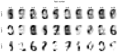
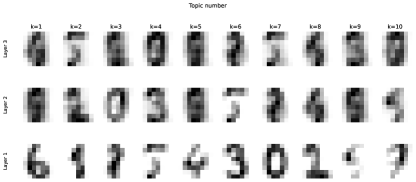
Chain 1	Chain 2
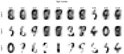
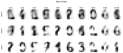
Chain 3	Chain 4

Figure S2: Hierarchy of topics learned by a three-layer multinomial belief network after training on the UC Irvine Machine Learning handwritten digits dataset. Layers (rows) consist of ten hidden units each and individual topics are represented by projection onto the pixels. Separate panels refer to individual Markov chains that were run in parallel.

To visualise the topic hierarchies learned by the MBN, we computed the projections from higher-level topics onto pixel activations. For each of the four Markov chains, Fig. S2 illustrates the projection from the top layer $\boldsymbol{\phi}^{(3)}\boldsymbol{\phi}^{(2)}\boldsymbol{\phi}^{(1)}$, the middle layer $\boldsymbol{\phi}^{(2)}\boldsymbol{\phi}^{(1)}$, and the bottom layer $\boldsymbol{\phi}^{(1)}$ onto the pixels.

S4-B Greedy layer-wise training on mutational signatures

For both the single layer PGBN and MBN, four chains were run for 1700 Gibbs steps each. Samples from the last 250 iterations, thinned every fifth sample, were collected for analysis (leaving 50 samples per chain). Thereafter, an additional 78-latent component layer was added on top of each respective model and the chains were run for an additional 500 steps. For the PGBN we inferred 38 latent components on the second layer (that is, out of all four chains, the smallest number of empty signatures $m_{{\underline{j}}k}^{(2)}=0$). The top layer was subsequently pruned back to 38 latent components and the chains were run for an additional 550 steps collecting the last 250 samples thinned to 50 samples. The MBN, was (accidentally) run slightly longer, for 750 steps, and we inferred 41 latent components. After pruning the empty topics, 250 additional steps were collected and thinned for analysis. Overall, a total of 77 days (78 days) of GPU time—divided across four nVidia A40 GPU devices—were used to execute 2700 Markov steps per chain for the MBN (2800 steps for the PGBN).

S4-C Meta-signature construction

Consensus meta-signatures were determined by matching the topics of different chains to its’ centroid by repeatedly solving the optimal transport problem [9] for the Jensen-Shannon distance (JSD) [9] using the Hungarian algorithm [10] until the centroid converged in terms of silhouette score [11], similar to Ref. [12]. The centroid was initialised to different chains and the consensus meta-signatures were selected that gave the best silhouette score. Finally, we selected robust meta-signatures by choosing those centroids where the JSD between the closest signature was no less than 0.25 across all chains, leaving four meta-signatures in total (named, M₁ through M₄). For completeness, we list all 37 other meta signatures in Figs. S4- S6. While completely inactive meta signatures were pruned, some remained with a very small topic activity throughout the dataset (to wit, M₂₃, M₂₆, M₃₅, M₃₇-M₄₀).

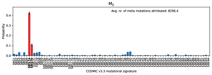
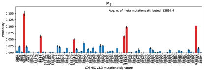
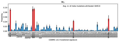
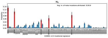
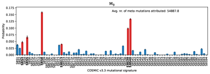
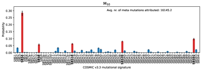
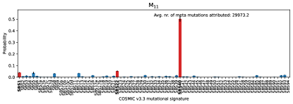
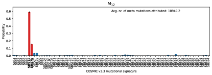
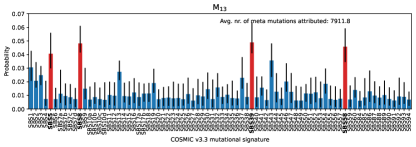
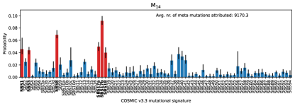
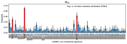
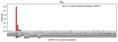
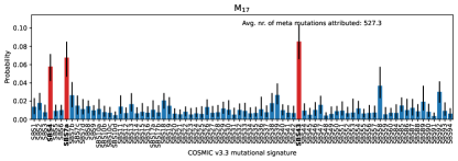
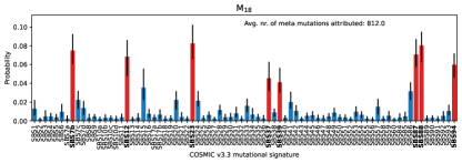
Figure S4: Posterior of meta-mutational signatures $k=\text{M}_{5},\dots,\text{M}_{18}$ for the multinomial believe network (meta signatures $k=\text{M}_{19},\dots,\text{M}_{41}$ are listed in subsequent figures). In each panel, the total number of meta signature $k$ counts $m^{(2)}_{k{\underline{j}}}$ (averaged over the posterior samples) is indicated as a measure of topic loading.

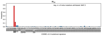
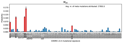
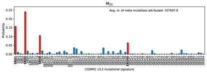
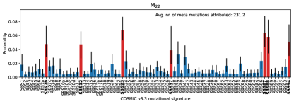
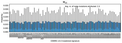
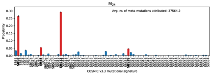
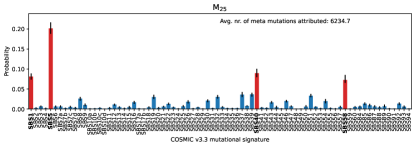
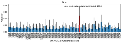
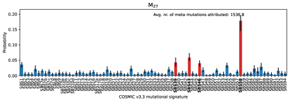
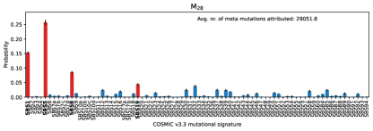
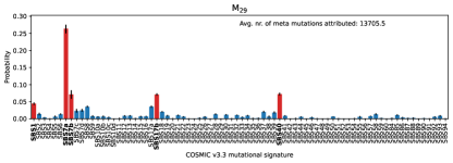
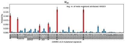
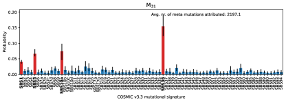
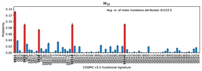
Figure S5: Continuation of Fig. S4 listing $k=\text{M}_{19},\dots,\text{M}_{32}$ (meta signatures $k=\text{M}_{33},\dots,\text{M}_{41}$ are listed in the subsequent figure).

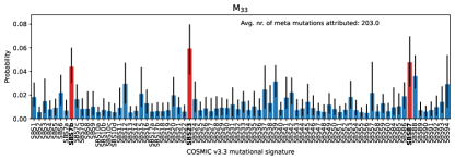
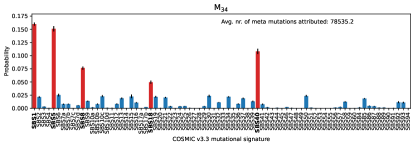
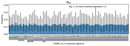
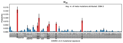
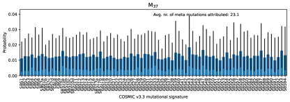
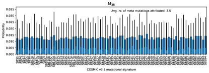
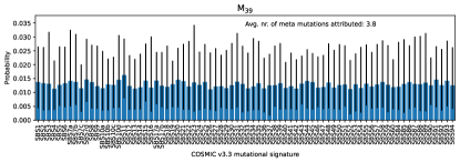
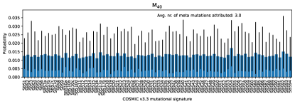
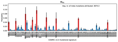
Figure S6: Continuation of Figs. S4 and S5 listing $k=\text{M}_{33},\dots,\text{M}_{41}$.

TABLE S2: Summary statistics of the hyperparameter $c^{(t)}$.

	mean	sd	hdi_3%	hdi_97%	mcse_mean	mcse_sd	ess_bulk	ess_tail	r_hat
$c^{(3)}$	0.298	0.036	0.230	0.351	0.016	0.012	5.0	12.0	3.10
$c^{(2)}$	33.978	4.545	26.305	39.319	2.125	1.611	5.0	13.0	3.73

TABLE S3: Summary statistics of the hyperparameter $\{r_{k}\}$ (top-level activation), per meta signature $k$.

Meta-signature	mean	sd	hdi_3%	hdi_97%	mcse_mean	mcse_sd	ess_bulk	ess_tail	r_hat
M1	0.0005	0.0003	0.0000	0.0011	0.0001	0.0001	7.8437	45.1667	1.5635
M2	0.0274	0.0171	0.0051	0.0489	0.0080	0.0060	5.2076	25.3881	2.9207
M3	0.0462	0.0275	0.0180	0.0934	0.0129	0.0098	5.2138	35.0239	2.8226
M4	0.0023	0.0009	0.0008	0.0037	0.0003	0.0002	7.2637	57.5069	1.6368
M5	0.0090	0.0091	0.0014	0.0255	0.0043	0.0032	5.6255	42.9691	2.3436
M6	0.0174	0.0141	0.0025	0.0425	0.0066	0.0050	5.1255	18.2017	3.0118
M7	0.0086	0.0077	0.0009	0.0208	0.0036	0.0027	5.9037	37.2047	2.1290
M8	0.0047	0.0056	0.0006	0.0154	0.0026	0.0020	7.2067	56.4231	1.6564
M9	0.0807	0.0395	0.0297	0.1444	0.0185	0.0140	5.1425	33.8033	2.9455
M10	0.0173	0.0102	0.0033	0.0298	0.0047	0.0036	5.6516	25.2606	2.3022
M11	0.0424	0.0294	0.0070	0.0889	0.0137	0.0104	5.2041	39.3170	2.8706
M12	0.0125	0.0045	0.0049	0.0189	0.0020	0.0015	5.4742	18.1715	2.4575
M13	0.0119	0.0190	0.0000	0.0463	0.0089	0.0067	5.3522	42.5339	2.6005
M14	0.0121	0.0108	0.0000	0.0307	0.0051	0.0038	5.1627	23.8320	2.9830
M15	0.0139	0.0141	0.0000	0.0335	0.0066	0.0050	5.3330	24.4206	2.6387
M16	0.0094	0.0015	0.0066	0.0121	0.0005	0.0004	8.5465	70.0544	1.4770
M17	0.0007	0.0005	0.0000	0.0017	0.0002	0.0002	6.3390	41.6786	1.8971
M18	0.0015	0.0009	0.0001	0.0029	0.0004	0.0003	6.1458	22.9947	1.9816
M19	0.0069	0.0036	0.0015	0.0117	0.0016	0.0012	5.9197	36.6124	2.0946
M20	0.0441	0.0335	0.0124	0.1036	0.0157	0.0119	5.0797	15.1183	3.1108
M21	0.2091	0.0914	0.1374	0.3724	0.0428	0.0324	5.2223	40.6697	2.7940
M22	0.0003	0.0003	0.0000	0.0009	0.0001	0.0001	8.9105	41.9669	1.4437
M23	0.0001	0.0001	0.0000	0.0003	0.0000	0.0000	17.0880	69.2559	1.1846
M24	0.0590	0.0462	0.0209	0.1413	0.0216	0.0164	5.4445	25.3216	2.4660
M25	0.0124	0.0071	0.0048	0.0249	0.0033	0.0025	5.8507	32.4049	2.1428
M26	0.0003	0.0003	0.0000	0.0010	0.0001	0.0001	8.8749	41.5220	1.4720
M27	0.0030	0.0019	0.0001	0.0056	0.0008	0.0006	5.8643	17.1875	2.1408
M28	0.0626	0.0459	0.0172	0.1442	0.0215	0.0163	5.1546	24.8252	2.9731
M29	0.0221	0.0235	0.0007	0.0601	0.0110	0.0083	5.5399	45.9551	2.4353
M30	0.0056	0.0035	0.0004	0.0101	0.0016	0.0012	5.3785	26.2501	2.5512
M31	0.0044	0.0070	0.0000	0.0175	0.0033	0.0025	6.0873	22.1597	2.0126
M32	0.0991	0.0535	0.0183	0.1604	0.0251	0.0190	5.2073	48.6473	2.8941
M33	0.0004	0.0003	0.0000	0.0010	0.0001	0.0001	8.3580	80.6760	1.4931
M34	0.1459	0.0950	0.0333	0.2602	0.0445	0.0338	5.1767	33.8603	2.9398
M35	0.0000	0.0001	0.0000	0.0002	0.0000	0.0000	115.4890	95.5287	1.0455
M36	0.0020	0.0017	0.0000	0.0050	0.0008	0.0006	5.4310	59.6550	2.5273
M37	0.0001	0.0001	0.0000	0.0003	0.0000	0.0000	13.4681	93.1817	1.2433
M38	0.0001	0.0001	0.0000	0.0002	0.0000	0.0000	78.6768	160.1208	1.0418
M39	0.0001	0.0001	0.0000	0.0003	0.0000	0.0000	20.6372	145.3196	1.1420
M40	0.0001	0.0001	0.0000	0.0002	0.0000	0.0000	14.2321	22.7601	1.2294
M41	0.0042	0.0057	0.0000	0.0150	0.0027	0.0020	5.4181	21.5255	2.5456

References

- [1] L. Alzubaidi, J. Bai, A. Al-Sabaawi, J. Santamaría, A. Albahri, B. Al-dabbagh, M. Fadhel, M. Manoufali, J. Zhang, A. Al-Timemy, Y. Duan, A. Abdullah, L. Farhan, Y. Lu, A. Gupta, F. Albu, A. Abbosh, and Y. Gu, “A survey on deep learning tools dealing with data scarcity: definitions, challenges, solutions, tips, and applications,” Journal of Big Data, vol. 10, 04 2023.
- [2] M. Abdar, F. Pourpanah, S. Hussain, D. Rezazadegan, L. Liu, M. Ghavamzadeh, P. Fieguth, X. Cao, A. Khosravi, U. R. Acharya, V. Makarenkov, and S. Nahavandi, “A review of uncertainty quantification in deep learning: Techniques, applications and challenges,” Information Fusion, vol. 76, pp. 243–297, 2021.
- [3] T. Emmanuel, T. M. Maupong, D. Mpoeleng, T. Semong, M. Banyatsang, and O. Tabona, “A survey on missing data in machine learning,” Journal of Big Data, vol. 8, 2021.
- [4] D. M. Blei, A. Y. Ng, and M. I. Jordan, “Latent Dirichlet Allocation,” J. Mach. Learn. Res., vol. 3, p. 993–1022, mar 2003.
- [5] G. Hinton, S. Osindero, and Y.-W. Teh, “A fast learning algorithm for deep belief nets,” Neural Comput., vol. 18, no. 7, pp. 1527–1554, 2006.
- [6] M. Zhou, Y. Cong, and B. Chen, “Augmentable gamma belief networks,” J. Mach. Learn. Res., vol. 17, no. 163, pp. 1–44, 2016.
- [7] D. P. Kingma and M. Welling, “Auto-encoding variational bayes,” in 2nd International Conference on Learning Representations, ICLR 2014, Banff, AB, Canada, April 14-16, 2014, Conference Track Proceedings, Y. Bengio and Y. LeCun, Eds., 2014.
- [8] T. Minka, “Estimating a Dirichlet distribution,” Ann. Phys., vol. 2000, no. 8, pp. 1–13, 2003.
- [9] C. P. George and H. Doss, “Principled Selection of Hyperparameters in the Latent Dirichlet Allocation Model,” J. Mach. Learn. Res., vol. 18, pp. 162:1–162:38, 2017.
- [10] Y. W. Teh, M. I. Jordan, M. J. Beal, and D. M. Blei, “Hierarchical dirichlet processes,” J. Am. Stat. Assoc., vol. 101, no. 476, pp. 1566–1581, 2006.
- [11] K. P. Murphy, Probabilistic machine learning: Advanced topics. MIT press, 2023.
- [12] C. Lee and D. J. Wilkinson, “A review of stochastic block models and extensions for graph clustering,” Appl. Netw. Sci., vol. 4, no. 1, pp. 1–50, 2019.
- [13] R. Ranganath, L. Tang, L. Charlin, and D. Blei, “Deep Exponential Families,” in Proceedings of the Eighteenth International Conference on Artificial Intelligence and Statistics, ser. Proceedings of Machine Learning Research, G. Lebanon and S. V. N. Vishwanathan, Eds., vol. 38. San Diego, California, USA: PMLR, 09–12 May 2015, pp. 762–771.
- [14] R. Ranganath, D. Tran, and D. Blei, “Hierarchical variational models,” in Proceedings of The 33rd International Conference on Machine Learning, ser. Proceedings of Machine Learning Research, M. F. Balcan and K. Q. Weinberger, Eds., vol. 48. New York, New York, USA: PMLR, 20–22 Jun 2016, pp. 324–333.
- [15] P. F. Ferreira, J. Kuipers, and N. Beerenwinkel, “Deep exponential families for single-cell data analysis,” bioRxiv, 2022.
- [16] H. Soleimani, J. Hensman, and S. Saria, “Scalable joint models for reliable uncertainty-aware event prediction,” IEEE T. Pattern Anal., vol. 40, no. 8, pp. 1948–1963, 2017.
- [17] D. M. Blei, A. Kucukelbir, and J. D. McAuliffe, “Variational inference: A review for statisticians,” J. Am. Stat. Assoc., vol. 112, no. 518, pp. 859–877, 2017.
- [18] H. Zhao, L. Du, W. Buntine, and M. Zhou, “Dirichlet belief networks for topic structure learning,” in Advances in Neural Information Processing Systems, S. Bengio, H. Wallach, H. Larochelle, K. Grauman, N. Cesa-Bianchi, and R. Garnett, Eds., vol. 31. Curran Associates, Inc., 2018.
- [19] R. Panda, A. Pensia, N. Mehta, M. Zhou, and P. Rai, “Deep topic models for multi-label learning,” in Proceedings of the Twenty-Second International Conference on Artificial Intelligence and Statistics, ser. Proceedings of Machine Learning Research, K. Chaudhuri and M. Sugiyama, Eds., vol. 89. PMLR, 16–18 Apr 2019, pp. 2849–2857.
- [20] Y.-A. Ma, T. Chen, and E. Fox, “A complete recipe for stochastic gradient mcmc,” in Advances in Neural Information Processing Systems, C. Cortes, N. Lawrence, D. Lee, M. Sugiyama, and R. Garnett, Eds., vol. 28. Curran Associates, Inc., 2015.
- [21] Y. Cong, B. Chen, H. Liu, and M. Zhou, “Deep latent Dirichlet allocation with topic-layer-adaptive stochastic gradient Riemannian MCMC,” in International conference on machine learning. PMLR, 2017, pp. 864–873.
- [22] H. Zhang, B. Chen, D. Guo, and M. Zhou, “Whai: Weibull hybrid autoencoding inference for deep topic modeling,” in ICLR, 2018.
- [23] H. Zhang, B. Chen, Y. Cong, D. Guo, H. Liu, and M. Zhou, “Deep autoencoding topic model with scalable hybrid bayesian inference,” IEEE T. Pattern Anal., vol. 43, no. 12, pp. 4306–4322, 2020.
- [24] W. Chen, B. Chen, Y. Liu, X. Cao, Q. Zhao, H. Zhang, and L. Tian, “Max-margin deep diverse latent Dirichlet allocation with continual learning,” IEEE T. Cybernetics, vol. 52, no. 7, pp. 5639–5653, 2021.
- [25] Y. Zhang, X. Jiang, A. J. Mentzer, G. McVean, and G. Lunter, “Topic modeling identifies novel genetic loci associated with multimorbidities in uk biobank,” Cell Genom., vol. 3, no. 8, 2023.
- [26] M. D. Escobar and M. West, “Bayesian density estimation and inference using mixtures,” J. Am. Stat. Assoc., vol. 90, no. 430, pp. 577–588, 1995.
- [27] M. Zhou, L. Hannah, D. Dunson, and L. Carin, “Beta-negative binomial process and poisson factor analysis,” in Proceedings of the Fifteenth International Conference on Artificial Intelligence and Statistics, ser. Proceedings of Machine Learning Research, N. D. Lawrence and M. Girolami, Eds., vol. 22. La Palma, Canary Islands: PMLR, 21–23 Apr 2012, pp. 1462–1471.
- [28] M. Zhou and L. Carin, “Negative binomial process count and mixture modeling.” IEEE T. Pattern Anal., vol. 37, no. 2, pp. 307–320, 2015.
- [29] D. D. Lee and H. S. Seung, “Learning the parts of objects by non-negative matrix factorization,” Nature, vol. 401, no. 6755, pp. 788–791, 1999.
- [30] A. Gelman, J. B. Carlin, H. S. Stern, D. B. Dunson, A. Vehtari, and D. B. Rubin, Bayesian Data Analysis. New York: Chapman and Hall/CRC, 2013.
- [31] E. Alpaydin and C. Kaynak, “Optical Recognition of Handwritten Digits,” UCI Machine Learning Repository, 1998, doi: 10.24432/C50P49.
- [32] F. Pedregosa, G. Varoquaux, A. Gramfort, V. Michel, B. Thirion, O. Grisel, M. Blondel, P. Prettenhofer, R. Weiss, V. Dubourg, J. Vanderplas, A. Passos, D. Cournapeau, M. Brucher, M. Perrot, and Édouard Duchesnay, “Scikit-learn: Machine Learning in Python,” J. Mach. Learn. Res., vol. 12, no. 85, pp. 2825–2830, 2011.
- [33] S. Talts, M. Betancourt, D. Simpson, A. Vehtari, and A. Gelman, “Validating bayesian inference algorithms with simulation-based calibration,” arXiv preprint arXiv:1804.06788, 2018.
- [34] V. K. Singh, A. Rastogi, X. Hu, Y. Wang, and S. De, “Mutational signature SBS8 predominantly arises due to late replication errors in cancer,” Commun. Biol., vol. 3, no. 1, p. 421, 2020.
- [35] S. W. Brady, A. M. Gout, and J. Zhang, “Therapeutic and prognostic insights from the analysis of cancer mutational signatures,” Trends Genet., vol. 38, no. 2, pp. 194–208, 2022.
- [36] J. G. Tate, S. Bamford, H. C. Jubb, Z. Sondka, D. M. Beare, N. Bindal, H. Boutselakis, C. G. Cole, C. Creatore, E. Dawson et al., “Cosmic: the catalogue of somatic mutations in cancer,” Nucleic Acids Res., vol. 47, no. D1, pp. D941–D947, 2019.
- [37] Cosmic, “Cosmic - catalogue of somatic mutations in cancer,” May 2023, accessed: 2023-10-12. [Online]. Available: https://cancer.sanger.ac.uk/cosmic
- [38] L. B. Alexandrov, J. Kim, N. J. Haradhvala, M. N. Huang, A. W. Tian Ng, Y. Wu, A. Boot, K. R. Covington, D. A. Gordenin, E. N. Bergstrom et al., “The repertoire of mutational signatures in human cancer,” Nature, vol. 578, no. 7793, pp. 94–101, 2020.
- [39] S. A. Islam, M. Díaz-Gay, Y. Wu, M. Barnes, R. Vangara, E. N. Bergstrom, Y. He, M. Vella, J. Wang, J. W. Teague et al., “Uncovering novel mutational signatures by de novo extraction with SigProfilerExtractor,” Cell Genom., vol. 2, no. 11, 2022.
- [40] A. Vehtari, A. Gelman, D. Simpson, B. Carpenter, and P.-C. Bürkner, “Rank-normalization, folding, and localization: An improved r-hat for assessing convergence of mcmc (with discussion),” Bayesian Anal., vol. 16, no. 2, pp. 667–718, 2021.
- [41] H.-D. Li, I. Cuevas, M. Zhang, C. Lu, M. M. Alam, Y.-X. Fu, M. J. You, E. A. Akbay, H. Zhang, D. H. Castrillon et al., “Polymerase-mediated ultramutagenesis in mice produces diverse cancers with high mutational load,” J. Clin. Invest., vol. 128, no. 9, pp. 4179–4191, 2018.
- [42] K. P. Hodel, M. J. Sun, N. Ungerleider, V. S. Park, L. G. Williams, D. L. Bauer, V. E. Immethun, J. Wang, Z. Suo, H. Lu et al., “POLE mutation spectra are shaped by the mutant allele identity, its abundance, and mismatch repair status,” Mol. Cell, vol. 78, no. 6, pp. 1166–1177, 2020.
- [43] B. Meier, N. V. Volkova, Y. Hong, P. Schofield, P. J. Campbell, M. Gerstung, and A. Gartner, “Mutational signatures of DNA mismatch repair deficiency in C. elegans and human cancers,” Genome Res., vol. 28, no. 5, pp. 666–675, 2018.
- [44] E. N. Bergstrom, M. N. Huang, U. Mahto, M. Barnes, M. R. Stratton, S. G. Rozen, and L. B. Alexandrov, “Sigprofilermatrixgenerator: a tool for visualizing and exploring patterns of small mutational events,” BMC Genomics, vol. 20, no. 1, pp. 1–12, 2019.
- [45] M. Secrier, X. Li, N. De Silva, M. D. Eldridge, G. Contino, J. Bornschein, S. MacRae, N. Grehan, M. O’Donovan, A. Miremadi et al., “Mutational signatures in esophageal adenocarcinoma define etiologically distinct subgroups with therapeutic relevance,” Nat. Genet., vol. 48, no. 10, pp. 1131–1141, 2016.
- [46] K. Nones, N. Waddell, N. Wayte, A.-M. Patch, P. Bailey, F. Newell, O. Holmes, J. L. Fink, M. C. Quinn, Y. H. Tang et al., “Genomic catastrophes frequently arise in esophageal adenocarcinoma and drive tumorigenesis,” Nat. Commun., vol. 5, no. 1, p. 5224, 2014.
- [47] M. Tomkova, J. Tomek, S. Kriaucionis, and B. Schuster-Böckler, “Mutational signature distribution varies with dna replication timing and strand asymmetry,” Genome Biol., vol. 19, no. 1, pp. 1–12, 2018.
- [48] A. R. Poetsch, S. J. Boulton, and N. M. Luscombe, “Genomic landscape of oxidative dna damage and repair reveals regioselective protection from mutagenesis,” Genome Biol., vol. 19, no. 1, pp. 1–23, 2018.
- [49] S. Christensen, B. Van der Roest, N. Besselink, R. Janssen, S. Boymans, J. W. Martens, M.-L. Yaspo, P. Priestley, E. Kuijk, E. Cuppen et al., “5-Fluorouracil treatment induces characteristic T¿G mutations in human cancer,” Nature Commun., vol. 10, no. 1, p. 4571, 2019.
- [50] J. E. Kucab, X. Zou, S. Morganella, M. Joel, A. S. Nanda, E. Nagy, C. Gomez, A. Degasperi, R. Harris, S. P. Jackson et al., “A compendium of mutational signatures of environmental agents,” Cell, vol. 177, no. 4, pp. 821–836, 2019.
- [51] S. Nik-Zainal, L. B. Alexandrov, D. C. Wedge, P. Van Loo, C. D. Greenman, K. Raine, D. Jones, J. Hinton, J. Marshall, L. A. Stebbings et al., “Mutational processes molding the genomes of 21 breast cancers,” Cell, vol. 149, no. 5, pp. 979–993, 2012.
- [52] L. B. Alexandrov, P. H. Jones, D. C. Wedge, J. E. Sale, P. J. Campbell, S. Nik-Zainal, and M. R. Stratton, “Clock-like mutational processes in human somatic cells,” Nat. Genet., vol. 47, no. 12, pp. 1402–1407, 2015.
- [53] B. Nie, W. Gan, F. Shi, G.-X. Hu, L.-G. Chen, H. Hayakawa, M. Sekiguchi, J.-P. Cai et al., “Age-dependent accumulation of 8-oxoguanine in the dna and rna in various rat tissues,” Oxid. Med. Cell. Longev., vol. 2013, 2013.
- [54] S. Nik-Zainal, H. Davies, J. Staaf, M. Ramakrishna, D. Glodzik, X. Zou, I. Martincorena, L. B. Alexandrov, S. Martin, D. C. Wedge et al., “Landscape of somatic mutations in 560 breast cancer whole-genome sequences,” Nature, vol. 534, no. 7605, pp. 47–54, 2016.
- [55] A. R. Lawson, F. Abascal, T. H. Coorens, Y. Hooks, L. O’Neill, C. Latimer, K. Raine, M. A. Sanders, A. Y. Warren, K. T. Mahbubani et al., “Extensive heterogeneity in somatic mutation and selection in the human bladder,” Science, vol. 370, no. 6512, pp. 75–82, 2020.
- [56] M. L. Hoang, C.-H. Chen, V. S. Sidorenko, J. He, K. G. Dickman, B. H. Yun, M. Moriya, N. Niknafs, C. Douville, R. Karchin et al., “Mutational signature of aristolochic acid exposure as revealed by whole-exome sequencing,” Sci. Transl. Med., vol. 5, no. 197, p. 197ra102, 2013.
- [57] S. L. Poon, S.-T. Pang, J. R. McPherson, W. Yu, K. K. Huang, P. Guan, W.-H. Weng, E. Y. Siew, Y. Liu, H. L. Heng et al., “Genome-wide mutational signatures of aristolochic acid and its application as a screening tool,” Science Transl. Med., vol. 5, no. 197, p. 197ra101, 2013.
- [58] S. Nik-Zainal, J. E. Kucab, S. Morganella, D. Glodzik, L. B. Alexandrov, V. M. Arlt, A. Weninger, M. Hollstein, M. R. Stratton, and D. H. Phillips, “The genome as a record of environmental exposure,” Mutagenesis, vol. 30, no. 6, pp. 763–770, 2015.
- [59] N. K. Hayward, J. S. Wilmott, N. Waddell, P. A. Johansson, M. A. Field, K. Nones, A.-M. Patch, H. Kakavand, L. B. Alexandrov, H. Burke et al., “Whole-genome landscapes of major melanoma subtypes,” Nature, vol. 545, no. 7653, pp. 175–180, 2017.
- [60] B. Li, S. W. Brady, X. Ma, S. Shen, Y. Zhang, Y. Li, K. Szlachta, L. Dong, Y. Liu, F. Yang et al., “Therapy-induced mutations drive the genomic landscape of relapsed acute lymphoblastic leukemia,” Blood-J. Hematol., vol. 135, no. 1, pp. 41–55, 2020.
- [61] H. C. Donker, B. van Es, M. Tamminga, G. A. Lunter, L. C. L. T. van Kempen, E. Schuuring, T. J. N. Hiltermann, and H. J. M. Groen, “Using genomic scars to select immunotherapy beneficiaries in advanced non-small cell lung cancer,” Sci. Rep., vol. 13, no. 1, p. 6581, 2023.
- [62] C. Pleguezuelos-Manzano, J. Puschhof, A. Rosendahl Huber, A. van Hoeck, H. M. Wood, J. Nomburg, C. Gurjao, F. Manders, G. Dalmasso, P. B. Stege et al., “Mutational signature in colorectal cancer caused by genotoxic pks+ E. coli,” Nature, vol. 580, no. 7802, pp. 269–273, 2020.
- [63] A. Boot, A. W. Ng, F. T. Chong, S.-C. Ho, W. Yu, D. S. Tan, N. G. Iyer, and S. G. Rozen, “Characterization of colibactin-associated mutational signature in an asian oral squamous cell carcinoma and in other mucosal tumor types,” Genome Res., vol. 30, no. 6, pp. 803–813, 2020.
- [64] H. Lee-Six, S. Olafsson, P. Ellis, R. J. Osborne, M. A. Sanders, L. Moore, N. Georgakopoulos, F. Torrente, A. Noorani, M. Goddard et al., “The landscape of somatic mutation in normal colorectal epithelial cells,” Nature, vol. 574, no. 7779, pp. 532–537, 2019.
- [65] J. Bradbury, R. Frostig, P. Hawkins, M. J. Johnson, C. Leary, D. Maclaurin, G. Necula, A. Paszke, J. VanderPlas, S. Wanderman-Milne, and Q. Zhang, “JAX: composable transformations of Python+NumPy programs,” 2018.

References

- [1] M. Zhou and L. Carin, “Negative binomial process count and mixture modeling.” IEEE T. Pattern Anal., vol. 37, no. 2, pp. 307–320, 2015.
- [2] C. E. Antoniak, “Mixtures of Dirichlet Processes with Applications to Bayesian Nonparametric Problems,” Ann. Stat., vol. 2, no. 6, pp. 1152 – 1174, 1974.
- [3] D. M. Blei, A. Y. Ng, and M. I. Jordan, “Latent Dirichlet Allocation,” J. Mach. Learn. Res., vol. 3, p. 993–1022, mar 2003.
- [4] M. Zhou, L. Hannah, D. Dunson, and L. Carin, “Beta-negative binomial process and poisson factor analysis,” in Proceedings of the Fifteenth International Conference on Artificial Intelligence and Statistics, ser. Proceedings of Machine Learning Research, N. D. Lawrence and M. Girolami, Eds., vol. 22. La Palma, Canary Islands: PMLR, 21–23 Apr 2012, pp. 1462–1471.
- [5] M. Zhou, Y. Cong, and B. Chen, “Augmentable gamma belief networks,” J. Mach. Learn. Res., vol. 17, no. 163, pp. 1–44, 2016.
- [6] T. Minka and J. Lafferty, “Expectation-Propagation for the generative aspect model,” in Proceedings of the 18th Conference on Uncertainty in Artificial Intelligence (UAI), San Francisco, CA, 2002.
- [7] Y. W. Teh, M. I. Jordan, M. J. Beal, and D. M. Blei, “Hierarchical dirichlet processes,” J. Am. Stat. Assoc., vol. 101, no. 476, pp. 1566–1581, 2006.
- [8] M. D. Escobar and M. West, “Bayesian density estimation and inference using mixtures,” J. Am. Stat. Assoc., vol. 90, no. 430, pp. 577–588, 1995.
- [9] K. P. Murphy, Probabilistic machine learning: Advanced topics. MIT press, 2023.
- [10] D. F. Crouse, “On implementing 2d rectangular assignment algorithms,” IEEE T. Aero. Elec. Sys., vol. 52, no. 4, pp. 1679–1696, 2016.
- [11] P. J. Rousseeuw, “Silhouettes: a graphical aid to the interpretation and validation of cluster analysis,” J. Comput. Appl. Math., vol. 20, pp. 53–65, 1987.
- [12] L. B. Alexandrov, J. Kim, N. J. Haradhvala, M. N. Huang, A. W. Tian Ng, Y. Wu, A. Boot, K. R. Covington, D. A. Gordenin, E. N. Bergstrom et al., “The repertoire of mutational signatures in human cancer,” Nature, vol. 578, no. 7793, pp. 94–101, 2020.