Lane-Keeping Control of Autonomous Vehicles Through a Soft-Constrained Iterative LQR

Abstract

The accurate prediction of smooth steering inputs is crucial for autonomous vehicle applications because control actions with jitter might cause the vehicle system to become unstable. To address this problem in automobile lane-keeping control without the use of additional smoothing algorithms, we developed a soft-constrained iterative linear–quadratic regulator (soft-CILQR) algorithm by integrating CILQR algorithm and a model predictive control (MPC) constraint relaxation method. We incorporated slack variables into the state and control barrier functions of the soft-CILQR solver to soften the constraints in the optimization process so that stabilizing control inputs can be calculated in a relatively simple manner. Two types of automotive lane-keeping experiments were conducted with a linear system dynamics model to test the performance of the proposed soft-CILQR algorithm and to compare its performance with that of the CILQR algorithm: numerical simulations and experiments involving challenging vision-based maneuvers. In the numerical simulations, the soft-CILQR and CILQR solvers managed to drive the system toward the reference state asymptotically; however, the soft-CILQR solver obtained smooth steering input trajectories more easily than did the CILQR solver under conditions involving additive disturbances. In the experiments with visual inputs, the soft-CILQR controller outperformed the CILQR controller in terms of tracking accuracy and steering smoothness during the driving of an ego vehicle on TORCS.

I Introduction

GeNERATING smooth control actions is a fundamental requirement in controller design because input jitter might increase the computational burden of actuators or even damage them. This problem has become crucial in practical applications. For example, the presence of various types of disturbances in vision-based vehicle control systems [1, 2, 3, 4] causes poor perception performance, which might result in the generation of jittery control predictions by the controller. For optimization-based controllers, a straightforward solution for the aforementioned problem involves employing smoothing algorithms, such as the Savitzky–Golay filter [5], to smooth control signals. However, such operations are not included in the optimization process; thus, control inputs might not be optimal. Studies have proposed rigorous approaches for the smoothing of control actions without the use of external smoothing algorithms. Examples of such approaches include those involving the tuning of the weighting matrices of control variables terms in model predictive control (MPC) cost functions [6], the regularization of policy output in a reinforcement-learning-based solution [7], and the addition of derivative action terms in the cost functions of a model predictive path integral control algorithm [8]. Stability can also be achieved using MPC schemes with softened (relaxed) constraints.

The authors of [9] formulated a soft-constrained MPC approach to handle infeasible optimization problems. They relaxed state constraints by introducing slack variables into the optimization process. They added a standard quadratic penalty term to the cost function to penalize excessively high values of slack variables. Consequently, their controller was determined to be less conservative and allowed temporal violations of constraints. Subsequently, the authors of [10] introduced an additional linear penalty term into the cost function [9] to remove counterintuitive solutions of the aforementioned controller. In [11], a procedure was proposed for computing the upper bound of the prediction horizon, and the corresponding finite-horizon soft-constrained MPC problem was solved under stability guarantees. For linear systems with polytopic constraints, the authors of [12] proposed a soft-constrained MPC approach that uses polytopic terminal sets and can guarantee asymptotic system stability. In [13], a soft-constrained MPC method was developed for linear systems; the model considers the general forms of the relaxed stage and terminal constraints. The novel feature of this method is that it involves the consideration of the terminal dynamics of the augmented state–slack variables, which guarantees a decrease in the terminal cost of the considered MPC problem.

The replacement of constraints with barrier functions can increase the stability of solutions for MPC problems [14]. In the MPC formulation developed in [14], weighted barrier functions that ensure that inequality constraints are strictly satisfied are included in the cost function. These barriers enable smooth control actions to be achieved when the system approaches constraint bounds. The authors of [15] leveraged relaxed barrier functions in linear MPC. This approach enables the enlargement of the feasible solution set for a hard-constrained MPC problem [14]. Through a numerical example, the authors of [15] showed that state trajectories can converge to the reference point in MPC schemes, even if the initial conditions are infeasible. Multiple studies [16, 17, 18] have investigated the use of barrier functions to shape system constraints in the context of the iterative linear–quadratic regulator (ILQR) algorithm [19, 20], resulting in the creation of a constrained ILQR (CILQR) algorithm; the CILQR algorithm has been used to solve motion planning problems for autonomous vehicles and has exhibited higher computation efficiency than the standard sequential quadratic programming (SQP) algorithm in these problems.

The present study presents a soft-CILQR algorithm, which integrates the CILQR algorithm and the soft-constrained MPC technique developed in [13]. We developed the proposed algorithm by using the research of [14] as a reference. Our goal was to develop an efficient lane-keeping controller that can generate smooth control actions for autonomous vehicles when functioning under disturbance. In this paper, control actions refer to the selection of appropriate vehicle steering angles. Because physical limits exist for the steering angle, the bounds of such angles are not relaxed in our algorithm. The slack variables are incorporated into the barrier functions for the steering angle and lateral offset constraints in the soft-CILQR solver, thereby enabling this solver to compute stabilizing control inputs when nonsmooth control actions are caused by disturbances. Therefore, the main contribution of this study is that it designed a soft-CILQR controller for the lane-keeping control of autonomous vehicles. We analyzed the behaviors of the proposed soft-CILQR solver under additive disturbances through numerical experiments by using a linear path-tracking model [2, 6, 22]. We also compared the performance of the soft-CILQR and CILQR solvers in the aforementioned experiments. Subsequently, vision-based simulations of autonomous driving were performed in TORCS [21] to validate the performance of the proposed soft-CILQR controller in terms of lane-keeping error and steering smoothness for controlled self-driving vehicles. Disturbances must be considered in examinations of autonomous driving because they may compromise driving comfort and driving safety.

The rest of the paper is organized as follows. The adopted path-tracking dynamic model is introduced in Section II. The proposed soft-CILQR algorithm is described in Section III. The experimental results and relevant discussion are provided in Section IV. Finally, the conclusions are presented in Section V.

II Dynamic Lane-Keeping Model

The objective of this study was to develop an efficient lane-keeping (path-tracking) control algorithm that can ensure the stability of autonomous vehicles. Therefore, a path-tracking model [2, 6, 22, 23] that uses lateral offset (the distance of the ego vehicle from the lane centerline, denoted as $\Delta$), heading angle (the orientation error between the car’s yaw angle and lane direction, denoted as $\theta$), and their derivatives to describe ego vehicle states was adopted in this study. This model is introduced in this section.

Consider the following: the ego car’s speed along the longitudinal (heading) direction is $v_{x}$, and its motion in the lateral direction has two degrees of freedom: the lateral position $y$ and yaw angle $\psi$. In this case, the lateral tire forces acting on the front ($f$) and real ($r$) wheels of the car can be expressed as follows:

$$F_{yf}=2C_{\alpha f}\left({\delta-\theta_{vf}}\right),$$ (1a)

$$F_{yr}=2C_{\alpha r}\left({-\theta_{vr}}\right),$$ (1b)

where $C_{\alpha f}$ and $C_{\alpha r}$ are the cornering stiffness values of the front and real tires, respectively; $\delta$ is the steering angle; and ${\theta_{vf}}$ and ${\theta_{vr}}$ are the angular velocities of the front and real tires, respectively. The term $\delta$ denotes the average value of the two front-wheel steering angles, and the distances traveled by these wheels are different. The small-angle approximation method can be used to calculate the tire velocity angles ${\theta_{vf}}$ and ${\theta_{vr}}$ as follows:

$$\theta_{vf}=\frac{{\dot{y}+l_{f}\dot{\psi}}}{{v_{x}}},$$ (2a)

$$\theta_{vr}=\frac{{\dot{y}-l_{r}\dot{\psi}}}{{v_{x}}},$$ (2b)

where $l_{f}$ and $l_{r}$ are the distances from the center of gravity of the vehicle to the front and rear tires, respectively. Newton’s second law of motion and a dynamic yaw equation can be used to represent $F_{yf}$ and $F_{yr}$ as follows:

$$F_{yf}+F_{yr}=m\left({\ddot{y}+v_{x}\dot{\psi}}\right)$$ (3)

and

$$l_{f}F_{yf}-l_{r}F_{yr}=I_{z}\ddot{\psi},$$ (4)

where $I_{z}$ is the moment of inertia along the $z$-axis. The road bank angle is ignored in the preceding equations.

To solve the vehicle path-tracking problem, the ego car’s lateral offset $\Delta$ and heading angle $\theta$ are defined as follows:

$$\ddot{\Delta}=\ddot{y}+v_{x}\left({\dot{\psi}-\dot{\psi}_{des}}\right),$$ (5a)

$$\theta=\psi-\psi_{des},$$ (5b)

where $\dot{\psi}_{des}=\kappa v_{x}$ is the desired yaw rate and $\kappa$ is the road curvature. The dynamic path-tracking model can be expressed as follows after the combination of Eqs. (3)–(5):

$$\begin{split}\ddot{\Delta}=&-\frac{{2C_{\alpha f}+2C_{\alpha r}}}{{mv_{x}}}\dot{\Delta}+\frac{{2C_{\alpha f}+2C_{\alpha r}}}{m}\theta\\ &-\frac{{2l_{f}C_{\alpha f}-2l_{r}C_{\alpha r}}}{{mv_{x}}}\dot{\theta}+\frac{{2C_{\alpha f}}}{m}\delta,\end{split}$$ (6a)

$$\begin{split}\ddot{\theta}=&-\frac{{2l_{f}C_{\alpha f}-2l_{r}C_{\alpha r}}}{{I_{z}v_{x}}}\dot{\Delta}+\frac{{2l_{f}C_{\alpha f}-2l_{r}C_{\alpha r}}}{{I_{z}}}\theta\\ &-\frac{{2l_{f}^{2}C_{\alpha f}+2l_{r}^{2}C_{\alpha r}}}{{I_{z}v_{x}}}\dot{\theta}+\frac{{2l_{f}C_{\alpha f}}}{{I_{z}}}\delta,\end{split}$$ (6b)

where $v_{x}$ is assumed to be constant and $\kappa$ is assumed to be small. To solve the aforementioned continuous-time model in an MPC framework, a tractable Euler integration scheme that allows real-time computation can be employed to discretize the model. The resulting discretized states are expressed as follows:

$$\Delta_{i+1}=\Delta_{i}+\dot{\Delta}_{i}dt,$$ (7a)

$$\dot{\Delta}_{i+1}=\dot{\Delta}_{i}+\ddot{\Delta}_{i}dt,$$ (7b)

$$\theta_{i+1}=\theta_{i}+\dot{\theta}_{i}dt,$$ (7c)

$$\dot{\theta}_{i+1}=\dot{\theta}_{i}+\ddot{\theta}_{i}dt,$$ (7d)

where $dt$ is the size of the discretization size and $i$ is the associated index. Thus, the following linear discrete-time path-tracking model is obtained [22]:

$${\bf x}_{i+1}\equiv{\bf f}\left({{\bf x}_{i},{\bf u}_{i}}\right)={\bf Ax}_{i}+{\bf Bu}_{i},$$ (8)

where the state vector and control input are defined as ${\bf x}\equiv\left[{\begin{array}[]{*{20}c}\Delta&{\dot{\Delta}}&\theta&{\dot{\theta}}\\ \end{array}}\right]^{T}$ and ${\bf u}\equiv\left[\delta\right]$, respectively. Moreover, the model matrices ar expressed as follows:

$${\bf A}=\left[{\begin{array}[]{*{20}c}{\alpha_{11}}&{\alpha_{12}}&0&0\\ 0&{\alpha_{22}}&{\alpha_{23}}&{\alpha_{24}}\\ 0&0&{\alpha_{33}}&{\alpha_{34}}\\ 0&{\alpha_{42}}&{\alpha_{43}}&{\alpha_{44}}\\ \end{array}}\right],\quad{\bf B}=\left[{\begin{array}[]{*{20}c}0\\ {\beta_{1}}\\ 0\\ {\beta_{2}}\\ \end{array}}\right].$$

The matrix coefficients are expressed as follows:

$$\begin{array}[]{l}\alpha_{11}=\alpha_{33}=1,\quad\alpha_{12}=\alpha_{34}=dt,\\ \alpha_{22}=1-\frac{{\left({2C_{\alpha f}+2C_{\alpha r}}\right)dt}}{{mv_{x}}},\quad\alpha_{23}=\frac{{\left({2C_{\alpha f}+2C_{\alpha r}}\right)dt}}{m},\\ \alpha_{24}=-\frac{{\left({2l_{f}C_{\alpha f}-2l_{r}C_{\alpha r}}\right)dt}}{{mv_{x}}},\quad\alpha_{42}=-\frac{{\left({2l_{f}C_{\alpha f}-2l_{r}C_{\alpha r}}\right)dt}}{{I_{z}v_{x}}},\\ \alpha_{43}=\frac{{\left({2l_{f}C_{\alpha f}-2l_{r}C_{\alpha r}}\right)dt}}{{I_{z}}},\quad\alpha_{44}=1-\frac{{\left({2l_{f}^{2}C_{\alpha f}+2l_{r}^{2}C_{\alpha r}}\right)dt}}{{I_{z}v_{x}}},\\ \beta_{1}={\frac{{2C_{\alpha f}dt}}{m}},\quad\beta_{2}=\frac{{2l_{f}C_{\alpha f}dt}}{{I_{z}}}.\\ \end{array}$$

The model and vehicle parameters used in this study are presented in Table I.

TABLE I: Values of the model and vehicle parameters used in this study

$dt$	0.01 s	$l_{f}$	1.27 m
$v_{x}$	20 m/s	$l_{r}$	1.37 m
$m$	1150 kg	${C_{\alpha f}}$	80000 N/rad
$I_{z}$	2000 kgm2	${C_{\alpha r}}$	80000 N/rad

III Soft-CILQR Algorithm

In this section, the soft-constrained MPC problem considered in this study is formulated on the basis of the model introduced in the previous section. The relevant constraints are then transformed into barrier functions, and the resulting unconstrained problem is solved using the proposed soft-CILQR algorithm. Finally, the upper bound of the prediction horizon of the examined MPC problem is calculated.

III-A Problem Formulation

The decision variables in the considered control problem are a sequence of states ${\bf X}\equiv\left\{{{\bf x}_{0},{\bf x}_{1},...,{\bf x}_{N}}\right\}$, a control sequence ${\bf U}\equiv\left\{{{\bf u}_{0},{\bf u}_{1},...,{\bf u}_{N-1}}\right\}$, and a slack sequence ${\bf E}\equiv\left\{{{\bf e}_{0},{\bf e}_{1},...,{\bf e}_{N}}\right\}$. The considered soft-constrained MPC problem is formulated as follows (Problem 1):

Problem 1:

$$\mathop{{\rm min}}\limits_{{\bf X},{\bf U},{\bf E}}J=J_{s}+J_{t},$$ (9a)

$$J_{s}=\sum\limits_{i=0}^{N-1}{{\bf x}_{i}^{T}{\bf Q}{{\bf x}_{i}}+{\bf u}_{i}^{T}{\bf Ru}_{i}}+{\bf e}_{i}^{T}{\bf Se}_{i},$$ (9b)

$$J_{t}=\sum\limits_{i=N}^{\bar{N}-1}{{\bf x}_{i}^{T}{\bf P}{{\bf x}_{i}}}+{\bf e}_{i}^{T}{\bf Te}_{i}$$ (9c)

subject to

$${\bf x}_{i+1}={\bf Ax}_{i}+{\bf Bu}_{i},\quad 0\leq i<N,$$ (10a)

$${\bf x}_{i+1}=\left({{\bf A}+{\bf B}{\bf K}}\right){\bf x}_{i},\quad N\leq i<\bar{N},$$ (10b)

$${\bf e}_{i+1}={\bf Me}_{i},\quad N\leq i<\bar{N},$$ (10c)

$$\left|\Delta\right|\leq\bar{\Delta}\left({1+\varepsilon_{l}}\right),$$ (10d)

$$\left|\delta\right|\leq\bar{\delta}\left({1+\varepsilon_{s}}\right),$$ (10e)

$$0\leq\varepsilon_{l}\leq\bar{\varepsilon_{l}},$$ (10f)

$$0\leq\varepsilon_{s}\leq\bar{\varepsilon_{s}},$$ (10g)

$$\left|{\dot{\Delta}}\right|\leq\dot{\Delta}_{\max},$$ (10h)

$$\left|\theta\right|\leq\theta_{\max},$$ (10i)

$$\left|{\dot{\theta}}\right|\leq\dot{\theta}_{\max},$$ (10j)

where $J_{s}$ and $J_{t}$ denote the stage and terminal cost functions, respectively. The weighting matrixes (${\bf Q}$, ${\bf R}$, ${\bf S}$, ${\bf P}$, and ${\bf T}$) are assumed to be symmetric positive-definite matrices. The terminal dynamics of the state vector ${\bf x}$ and slack vector ${\bf e}\equiv\left[{\begin{array}[]{*{20}c}{\varepsilon_{l}}&{\varepsilon_{s}}\\ \end{array}}\right]^{T}$ are expressed in Eqs. (10b) and (10c), respectively. The slack vector is proposed in [13] for linear systems. The prediction horizon is divided into two operating modes: the stage and terminal modes. The stage mode involves the prediction of variables over the first $N$ time steps, whereas the terminal mode involves the prediction of variables in the subsequent steps. In the terminal mode, predicted control inputs are specified by an unconstrained control law. The integer $\bar{N}$ denotes the upper bound of the prediction horizon. The matrix ${\bf P}$ is the solution of the discrete-time algebraic Riccati equation, which is expressed as follows:

$${\bf P}={\bf A}^{T}{\bf PA}+{\bf Q}-{\bf A}^{T}{\bf PB}({\bf B}^{T}{\bf PB}+{\bf R})^{-1}{\bf B}^{T}{\bf PA}.$$ (11)

The corresponding feedback gain ${\bf K}$ has the following form:

$${\bf K}=-\left({{\bf B}^{T}{\bf PB}+{\bf R}}\right)^{-1}{\bf B}^{T}{\bf PA}.$$ (12)

It is important to note that the matrix ${\bf P}$ also satisfies the Lyapunov equation, which is expressed as follows:

$${\bf P}=\left({{\bf A}+{\bf BK}}\right)^{T}{\bf P}\left({{\bf A}+{\bf BK}}\right)+{\bf Q}+{\bf K}^{T}{\bf RK}.$$ (13)

The following assumptions are made: ${\bf S}=S{\bf I}_{2}$, ${\bf T}=T{\bf I}_{2}$, and ${\bf M}=M{\bf I}_{2}$. The scalars $S$, $M\in\left[0,1\right)$, and $T=S/(1-M^{2})$ are designed to induce desirable asymptotic behaviors of the relaxed constraints [13]. For the inequality constraints expressed in Eqs. (10d) and (10e), $\bar{\Delta}\equiv{{\Delta_{\max}}\mathord{\left/{\vphantom{{\Delta_{\max}}{\left({1+\bar{\varepsilon_{l}}}\right)}}}\right.\kern-1.2pt}{\left({1+\bar{\varepsilon_{l}}}\right)}}$, and ${{\bar{\delta}\equiv\delta_{\max}}\mathord{\left/{\vphantom{{\bar{\delta}=\delta_{\max}}{\left({1+\bar{\varepsilon_{s}}}\right)}}}\right.\kern-1.2pt}{\left({1+\bar{\varepsilon_{s}}}\right)}}$; moreover, $\Delta_{\max}$ and $\delta_{\max}$ are the physical limitations of $\Delta$ and $\delta$, respectively. The nonnegative slack variables $\varepsilon_{l}$ and $\varepsilon_{s}$ have the upper bounds $\bar{\varepsilon_{l}}$ and $\bar{\varepsilon_{s}}$, respectively, in Eqs. (10f) and (10g). Thus, the values of $\Delta$ and $\delta$ are restricted to their bounds $\pm\Delta_{\max}$ and $\pm\delta_{\max}$, respectively, in the optimization process, even if slack variables are incorporated into this process. Finally, Eqs. (10h), (10i), and (10j) represent the constraints for the state variables ${\dot{\Delta}}$, $\theta$, and ${\dot{\theta}}$, respectively, the upper bounds of which are denoted as ${\dot{\Delta}}_{\max}$, $\theta_{\max}$, and ${\dot{\theta}}_{\max}$, respectively. The control-related parameters and constraints in this study are presented in Table II.

TABLE II: Control parameter values and constraints

${\bf Q}$	${\rm diag}\left({20,1,20,1}\right)$	$\Delta_{\max}$	2.0 m
${\bf R}$	$\left[60\right]$	$\dot{\Delta}_{\max}$	5.0 m/s
$(q_{l1},q_{l2})$	$(5,1)$	$\theta_{\max}$	$\pi/2$ rad
$(q_{s1},q_{s2})$	$(80,1)$	$\dot{\theta}_{\max}$	0.5 rad/s
$S$	0.01	$\delta_{\max}$	$\pi/6$ rad
$M$	0.9	$\varepsilon_{\max}$	19,…, 99

III-B Trajectory Optimizer

Barrier functions that ensure constraints satisfaction can be incorporated into Problem 1 to convert this problem into an effectively unconstrained optimization problem (i.e., Problem 2). Herein, constraints are modeled using exponential barrier functions, which are strictly convex and smooth functions [16, 24]. Therefore, the explicit form of Problem 2 is expressed as follows:

Problem 2:

$$\mathop{{\rm min}}\limits_{{\bf X},{\bf U},{\bf E}}{\tilde{J}}=J+J_{e}+J_{la}+J_{st}+J_{th},$$ (14a)

$$J_{e}=\sum\limits_{k=l,s}{\sum\limits_{i=0}^{N}{\exp\left({-\varepsilon_{k,i}}\right)+\exp\left({\varepsilon_{k,i}-\bar{\varepsilon_{k}}}\right)}},$$ (14b)

$$\begin{split}J_{la}=\sum\limits_{i=0}^{N}&{q_{l1}\exp\left\{{q_{l2}\left[{-\bar{\Delta}\left({1+\varepsilon_{l,i}}\right)-\Delta_{i}}\right]}\right\}}\\ &+q_{l1}\exp\left\{{q_{l2}\left[{\Delta_{i}-\bar{\Delta}\left({1+\varepsilon_{l,i}}\right)}\right]}\right\},\end{split}$$ (14c)

$$\begin{split}J_{st}=\sum\limits_{i=0}^{N-1}&{q_{s1}\exp\left\{{q_{s2}\left[{-\bar{\delta}\left({1+\varepsilon_{s,i}}\right)-\delta_{i}}\right]}\right\}}\\ &+q_{s1}\exp\left\{{q_{s2}\left[{\delta_{i}-\bar{\delta}\left({1+\varepsilon_{s,i}}\right)}\right]}\right\},\end{split}$$ (14d)

$$J_{th}=\sum\limits_{k=1}^{3}{\sum\limits_{i=0}^{N}{\exp\left({-x_{k,\max}-x_{k,i}}\right)+\exp\left({x_{k,i}-x_{k,\max}}\right)}}$$ (14e)

subject to

$$(10{\rm a}),\quad(10{\rm b}),\quad(10{\rm c}),$$

where $q_{s1,2}$ and $q_{l1,2}$ are barrier function parameters. Moreover, $x_{1}$, $x_{2}$, and $x_{3}$ represent ${\dot{\Delta}}$, $\theta$, and ${\dot{\theta}}$, respectively. Herein, $\bar{\varepsilon_{l}}=\bar{\varepsilon_{s}}\equiv\varepsilon_{\max}$ is assumed for simplicity.

To solve Problem 2, the ILQR algorithm is employed to compute updated state and control variables. The ILQR solver performs alternating backward and forward propagation steps to optimize the control strategy iteratively. In a backward propagation procedure, the control gains ${\bf\tilde{K}}_{i}$ and ${\bf\tilde{k}}_{i}$ are estimated using the analytical expressions of the expansion coefficients of the perturbed value function presented in [25, 26]. The improved state and control sequences can then be obtained in a forward propagation process as follows:

$${\bf\hat{u}}_{i}={\bf u}_{i}+{\bf\tilde{k}}_{i}+{\bf\tilde{K}}_{i}\left({{\bf\hat{x}}_{i}-{\bf x}_{i}}\right),$$ (15a)

$${\bf\hat{x}}_{i+1}={\bf f}\left({{\bf\hat{x}}_{i},{\bf\hat{u}}_{i}}\right),$$ (15b)

where ${\bf\hat{x}}_{0}={\bf x}_{0}$. Moreover, herein, elements of the slack sequence are designed to be updated using the Newton descent method. Studies have indicated that a Newton-based optimizer can rapidly decay the cost function of barrier-function-based MPC problems [27, 28]. The relevant update law is expressed as follows:

$${\bf\hat{e}}_{i}={\bf e}_{i}-\left[{{\bf H}\tilde{J}\left({{\bf e}_{i}}\right)}\right]^{-1}\nabla\tilde{J}\left({{\bf e}_{i}}\right),$$ (16)

where the Hessian matrix ${\bf H}\tilde{J}\left({{\bf e}_{i}}\right)\succ 0$. The aforementioned procedures for the computation of the optimal state, control, and slack variables constitute the basis of the proposed soft-CILQR optimizer.

In summary, the main innovation aspect of the soft-CILQR algorithm is that it incorporates slack variables into the framework of the CILQR algorithm. This constraint-softening approach facilitates the achievement of control stability and preserves the high computation efficiency of the CILQR algorithm in real-time applications. The method used in the soft-CILQR algorithm to calculate the upper bound of the prediction horizon ${\bar{N}}$ is described in the following section.

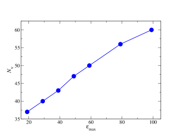
Figure 1: Relationship between $\varepsilon_{\max}$ and the computed $N_{\nu}$ value.

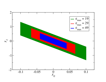
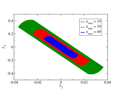
Figure 2: Visualization of $\chi_{MPI}$ for subsystems ($x_{0}$, $x_{1}$) = (${\Delta}$, ${\dot{\Delta}}$) and ($x_{2}$, $x_{3}$) = ($\theta$, ${\dot{\theta}}$) under $\varepsilon_{\max}$ values of 19, 29 and 49.

III-C Computation of the Upper Bound of the Prediction Horizon

The classic infinite-horizon MPC problem is solved by minimizing the infinite-dimensional cost function, which is computationally intractable in practice [11, 29]. Therefore, an upper bound must be calculated for the prediction horizon of the considered MPC problem. As described in the previous section, the prediction horizon of Problem 1 is divided into two operating modes: the stage and terminal modes. To ensure that the predictions made in the terminal mode satisfy the state, control, and slack constraints, the end state of the stage mode should lie in a positively invariant set $\chi_{T}$ under the dynamics defined by the state feedback control law ${\bf u}={\bf Kx}$, Eq. (10b), and Eq. (10c) with the following mixed constraint for the augmented state ${\bf\tilde{x}}\equiv\left[{\begin{array}[]{*{20}c}{\bf x}&{\bf e}\\ \end{array}}\right]^{T}$ [13]:

$${\bf\tilde{F}\tilde{x}}+{\bf\tilde{G}u}\leq{\bf\tilde{h}}.$$ (17)

The corresponding constraint matrices are expressed as follows:

$${\bf\tilde{F}}=\left({\begin{array}[]{*{20}c}{-1}&0&0&0&0&0\\ 1&0&0&0&0&0\\ 0&{-1}&0&0&0&0\\ 0&1&0&0&0&0\\ 0&0&{-1}&0&0&0\\ 0&0&1&0&0&0\\ 0&0&0&{-1}&0&0\\ 0&0&0&1&0&0\\ 0&0&0&0&0&0\\ 0&0&0&0&0&0\\ 0&0&0&0&{-1}&0\\ 0&0&0&0&1&0\\ 0&0&0&0&0&{-1}\\ 0&0&0&0&0&1\\ {-1}&0&0&0&{-\bar{\Delta}}&0\\ 1&0&0&0&{-\bar{\Delta}}&0\\ {-K_{0}}&{-K_{1}}&{-K_{2}}&{-K_{3}}&0&{-\bar{\delta}}\\ {K_{0}}&{K_{1}}&{K_{2}}&{K_{3}}&0&{-\bar{\delta}}\\ \end{array}}\right),$$

$${\bf\tilde{G}}=\left({\begin{array}[]{*{20}c}0\\ 0\\ 0\\ 0\\ 0\\ 0\\ 0\\ 0\\ {-1}\\ {1}\\ 0\\ 0\\ 0\\ 0\\ 0\\ 0\\ 0\\ 0\\ \end{array}}\right),\quad{\bf\tilde{h}}=\left({\begin{array}[]{*{20}c}{\Delta_{\max}}\\ {\Delta_{\max}}\\ {\dot{\Delta}_{\max}}\\ {\dot{\Delta}_{\max}}\\ {\theta_{\max}}\\ {\theta_{\max}}\\ {\dot{\theta}_{\max}}\\ {\dot{\theta}_{\max}}\\ {\delta_{\max}}\\ {\delta_{\max}}\\ 0\\ {\varepsilon_{\max}}\\ 0\\ {\varepsilon_{\max}}\\ {\bar{\Delta}}\\ {\bar{\Delta}}\\ {\bar{\delta}}\\ {\bar{\delta}}\\ \end{array}}\right).$$

To increase the applicability of the examined control problem, $\chi_{T}$ must be selected as the maximal positively invariant (MPI) set. The MPI set, denoted as $\chi_{MPI}$, is a polytope that can be expressed as follows [29]:

$$\chi_{MPI}\equiv\left\{{{\bf\tilde{x}}:({\bf\tilde{F}}+{\bf\tilde{G}\tilde{K}})({\bf\tilde{A}}+{\bf\tilde{B}\tilde{K}})^{i}{\bf\tilde{x}}\leq{\bf\tilde{h}},\quad i=0,...,N_{\nu}}\right\}.$$ (18)

The corresponding augmented state and control matrices are expressed as follows:

$${\bf\tilde{A}}=\left({\begin{array}[]{*{20}c}{\alpha_{11}}&{\alpha_{12}}&0&0&0&0\\ 0&{\alpha_{22}}&{\alpha_{23}}&{\alpha_{24}}&0&0\\ 0&0&{\alpha_{33}}&{\alpha_{34}}&0&0\\ 0&{\alpha_{42}}&{\alpha_{43}}&{\alpha_{44}}&0&0\\ 0&0&0&0&M&0\\ 0&0&0&0&0&M\\ \end{array}}\right),$$

$${\bf\tilde{B}}=\left({\begin{array}[]{*{20}c}0\\ {\beta_{1}}\\ 0\\ {\beta_{2}}\\ 0\\ 0\\ \end{array}}\right),\quad{\bf\tilde{K}}=\left({\begin{array}[]{*{20}c}{K_{0}}\\ {K_{1}}\\ {K_{2}}\\ {K_{3}}\\ 0\\ 0\\ \end{array}}\right)^{T},$$

where $K_{0,1,2,3}$ are components of $\bf K$. The relationship among the smallest positive integer $N_{\nu}$, $N$, and $\bar{N}$ in Problem 1 can be expressed as follows: $\bar{N}=N+N_{\nu}+1$. The smallest integer can be obtained by solving the following linear programming problem:

$$\mathop{{\rm max}}\limits_{\bf\tilde{x}}\left({{\bf\tilde{F}}+{\bf\tilde{G}\tilde{K}}}\right)_{j}\left({{\bf\tilde{A}}+{\bf\tilde{B}\tilde{K}}}\right)^{n+1}{\bf\tilde{x}},\quad j=1,...,n_{c}$$ (19)

subject to

$$\left({{\bf\tilde{F}}+{\bf\tilde{G}\tilde{K}}}\right)\left({{\bf\tilde{A}}+{\bf\tilde{B}\tilde{K}}}\right)^{i}{\bf\tilde{x}}\leq{\bf\tilde{h}},\quad i=0,...,n.$$ (20)

where $n_{c}$ is the row number in the matrix (${{\bf\tilde{F}}+{\bf\tilde{G}\tilde{K}}}$) and $n$ = 1,…, $N_{\nu}$. On the basis of the parameters and constraints defined in Tables I and II, the values of $N_{\nu}$ can be calculated for a system with $\varepsilon_{\max}$ = 19, 29, 39, 49, 59, 79, and 99 (Fig. 1). The calculation results indicate a nearly linear relationship between $N_{\nu}$ and $\varepsilon_{\max}$. Fig. 2 illustrates a visualization of $\chi_{MPI}$ for $\varepsilon_{\max}$ = 19, 29, and 49. The set $\chi_{MPI}$ becomes smaller as $\varepsilon_{\max}$ increases, and all the obtained $\chi_{MPI}$ sets fully adhere to the constraints defined in Table II. The above method, which involves using the unconstrained LQR gain, for calculating the upper bound of the prediction horizon can be performed offline and thus does not increase the online computational burden.

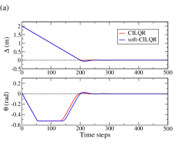
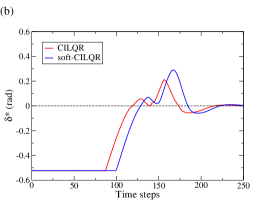
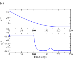
Figure 3: Numerical simulations results obtained when $\sigma$ = 0, $N$ = 40, and $\varepsilon_{\max}$ = 49. (a) Trajectories of $\Delta$ and $\theta$. Trajectories of the first component of the optimal (b) steering angle and (c) slack sequences. The broken lines represent reference data points (zeros).

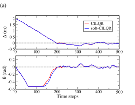
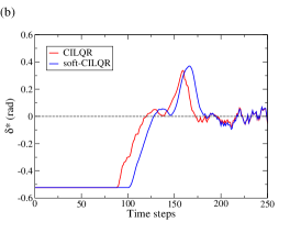
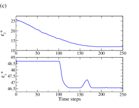
Figure 4: Numerical simulations results obtained when $\sigma$ = 1, $N$ = 40, and $\varepsilon_{\max}$ = 49. (a) Trajectories of $\Delta$ and $\theta$. Trajectories of the first component of the optimal (b) steering angle and (c) slack sequences.

IV Experimental Results and Discussion

To test the proposed soft-CILQR algorithm, first, numerical simulations were conducted to analyze its performance in the presence of bounded additive disturbances. Second, vision-based vehicle lane-keeping simulations were performed on TORCS to validate the performance of the proposed algorithm in self-driving scenarios. The vision-based experiments were more challenging than the numerical experiments because the vision-based experiments involved more uncertainties with respect to model inputs and were more similar to real-world scenarios. For performance comparison, the CILQR algorithm was also used in the aforementioned experiments under the same settings as those used for the proposed algorithm. All experiments were conducted on a desktop PC with a 3.6-GHz Intel i9-9900K CPU, an Nvidia RTX 2080 Ti graphics processing unit, and 64 GB RAM. The proposed soft-CILQR algorithm achieved an average runtime of 2.55 ms and is thus applicable in real-time autonomous driving scenarios.

IV-A Numerical Simulations

The numerical simulations involved controlling an autonomous vehicle [Eq. (8)] by using the soft-CILQR and CILQR solvers under the additive disturbance ${\bf w}=\left[{\begin{array}[]{*{20}c}{w_{0}}&{w_{1}}&{w_{2}}&{w_{3}}\\ \end{array}}\right]^{T}$. The constraints of ${\bf w}$ are expressed as follows:

$$\begin{array}[]{l}\left|{w_{0}}\right|\leq 0.013\quad{\rm m},\\ \left|{w_{1}}\right|\leq 0.325\quad{\rm m/s},\\ \left|{w_{2}}\right|\leq 0.010\quad{\rm rad},\\ \left|{w_{3}}\right|\leq 0.170\quad{\rm rad/s}.\\ \end{array}$$ (21)

These constraints are similar to those used in [6]. At each simulation time step ($t$), the solvers were initialized by setting the control and slack sequences to zeros. Moreover, the current state was set as follows:

$${\bf x}_{t}={\bf f}\left({{\bf x}_{t-1},{\bf u}_{t-1}^{*}}\right)+\sigma{\bf w}_{t},$$ (22)

where ${\bf u}_{t-1}^{*}=\left[{\delta_{t-1}^{*}}\right]$ is the first element of the optimal steering angle sequence of the last iteration, ${\bf w}_{t}$ is disturbance caused by uniformly distributed noise in the current sampling step, and $\sigma$ is the corresponding noise level. Here, ${\bf w}$ can be external disturbances, uncertainties, model deviations, or measurement errors. The selected initial state was ${\bf x}_{0}=\left[{\begin{array}[]{*{20}c}2&0&0&0\\ \end{array}}\right]^{T}$, and the parameter and constraint values listed in Tables I and II were used. To test algorithm performance in the presence of disturbances, three noise levels ($\sigma$ = 0, 1, and 2) were considered.

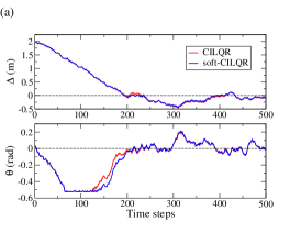
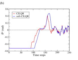
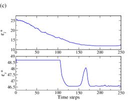
Figure 5: Numerical simulations results obtained when $\sigma$ = 2, $N$ = 40, and $\varepsilon_{\max}$ = 49. (a) Trajectories of $\Delta$ and $\theta$. Trajectories of the first component of the optimal (b) steering angle and (c) slack sequences.

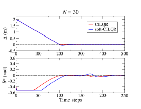
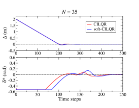
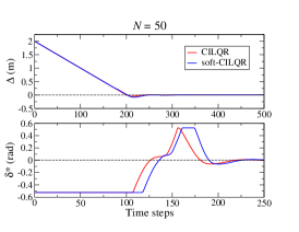
Figure 6: Numerical simulation results obtained for the trajectories of $\Delta$ by using the soft-CILQR solver when $\sigma$ = 0, $\varepsilon_{\max}$ = 49, and $N$ = 30, 35, 50.

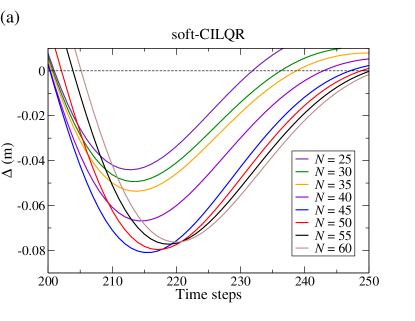
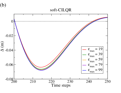
Figure 7: Numerical simulation results obtained for the trajectories of $\Delta$ by using the soft-CILQR solver. (a) When $\sigma$ = 0, $\varepsilon_{\max}$ = 49, and $N$ had different values. The broken lines represent reference data points (zeros). The minimum values of $\Delta$ were -0.0440, -0.0668, -0.0809, -0.0796, -0.0772, and -0.0763 m when $N$ = 25, 40, 45, 50, 55, and 60, respectively. (b) When $\sigma$ = 0, $N$ = 40, and $\varepsilon_{\max}$ had various values. The minimum values of $\Delta$ were -0.0635, -0.0662, -0.0671, -0.0676, and -0.0678 m when $\varepsilon_{\max}$ = 19, 39, 59, 79, and 99, respectively.

Fig. 3(a) presents the $\Delta$ and $\theta$ trajectories generated by the soft-CILQR and CILQR solvers when $\sigma$ = 0, indicating that both algorithms were able to control the vehicle system asymptotically to enable it to reach the reference point (${\bf 0}$). Moreover, the soft-CILQR controller with relaxed constraints is less conservative than the CILQR controller; the trajectory obtained for $\Delta$ by using the soft-CILQR solver reached the target point earlier than did that obtained for $\Delta$ by using the CILQR solver. When the noise level increased to $\sigma$ = 1 and 2 [Fig. 4(a) and Fig. 5(a), respectively], the control performance of both algorithms was poor. The system exhibited obvious instability when the state trajectory approached points near $t=200$, where the magnitude of the state vector ${\bf x}$ was close to that of the disturbance. The trajectories obtained using the CILQR and soft-CILQR algorithms exhibited similar behaviors at long times, and the maximum $\Delta$ deviation between the two methods was approximately 0.24 and 0.46 m when $\sigma$ = 1 and 2, respectively.

Fig. 3(b), Fig. 4(b), and Fig. 5(b) illustrate the trajectories obtained for the optimal steering angle ($\delta^{*}$) when $\sigma$ = 0, 1, and 2, respectively. The $\delta^{*}$ values were clipped for short times ($t<$ 100) to prevent the steering signal from exceeding the relevant physical limitation ($-\pi/6$). Compared with the solution curves obtained using the CILQR algorithm, those obtained using the soft-CILQR algorithm exhibited greater overshoot around $t$ = 170. A similar behavior was also observed in [15], in which the overshoot of the control input curve increased with the extent of constraint relaxation. As $\sigma$ increased, the overshoot and steady-state errors exhibited by both algorithms increased. Fig. 3(c), Fig. 4(c), and Fig. 5(c) display the trajectories of the first element of the optimal slack sequences, that is, ${\bf e}^{*}=\left[{\begin{array}[]{*{20}c}{\varepsilon_{l}^{*}}&{\varepsilon_{s}^{*}}\\ \end{array}}\right]^{T}$. Overall, the ${\varepsilon_{l}^{*}}$ and ${\varepsilon_{s}^{*}}$ trajectories did not exceed their corresponding upper limits ($\varepsilon_{\max}$ = 49). The ${\varepsilon_{s}^{*}}$ trajectories exhibited overshoot at around $t$ = 170, and the extent of overshoot increased with $\sigma$. This overshoot corresponded to the overshoots of the $\delta^{*}$ curves displayed in Fig. 3(b), Fig. 4(b), and Fig. 5(b) at the same time step. In particular, the soft-CILQR solver yielded smoother $\delta^{*}$ curves than did the CILQR solver when 100 $<t<$ 200 [Fig. 3(b), Fig. 4(b), and Fig. 5(b)].

The $\Delta$ and $\delta^{*}$ trajectories obtained when $\sigma$ = 0 at different values of $N$ (30, 35, and 50) were compared (Fig. 6), and the results indicated that the maximum $\delta^{*}$ value increased with $N$. The maximum $\delta^{*}$ values produced by the soft-CILQR solver at an $N$ value of 50 were clipped [Fig. 6(c)] because some of these values exceeded the upper bound of the steering angle ($\pi/6$). Fig. 7(a) illustrates the evolution of the solution trajectories obtained for $\Delta$ by using the soft-CILQR solver when 200 $<t<$ 250 at $N$ values ranging from 25 to 60. An increase in $N$ from 25 to 45 resulted in the generation of less conservative trajectories; however, as displayed in Fig. 6(c), the clipping of the $\delta^{*}$ values obtained at an $N$ value of 50 resulted in the generation of more conservative $\Delta$ trajectories. Consequently, the maximum deviation in the $\Delta$ values decreased as $N$ increased beyond 50. Fig. 7(b) presents the evolution of the $\Delta$ trajectories obtained at $\varepsilon_{\max}$ values ranging from 19 to 99. The maximum deviation of the $\Delta$ values increased with $\varepsilon_{\max}$. Because of the existence of an approximately linear relationship between $\varepsilon_{\max}$ and $N_{\nu}$ (Fig. 1), the soft-CILQR solver provided less conservative trajectories as $N_{\nu}$ and $N$ increased. On the basis of the numerical simulation results, we used an $N$ value of 40 and an $\varepsilon_{\max}$ value of 49 in the vision-based experiments.

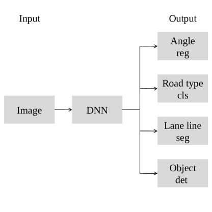
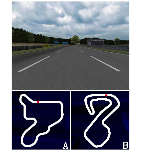
Figure 8: Illustration of the vision-based driving simulations. (Left) Perception module. (Right) Example traffic scene on TORCS and testing tracks A and B. The red symbols on the track maps represent the starting locations of the ego vehicle, which had a counterclockwise driving direction.

IV-B Vision-Based Lane-Keeping Experiments

The development of deep neural network (DNN)-based methods in the past decade has enhanced the performance of machine vision systems in autonomous driving applications. In addition, vision-based autonomous driving methods that involve using cameras for environment perception are cheaper than those that involve the use of expensive LiDAR sensors [1, 4]. However, the susceptibility of visual perception systems to adverse driving conditions often results in control instability for self-driving vehicles [2]. Accordingly, this study conducted vision-based lateral control experiments to validate the performance of the proposed soft-CILQR algorithm and to compare its performance with that of the CILQR algorithm.

TABLE III: Performance of the CILQR and soft-CILQR algorithmss in the vision-based experiments

Exp.	Track	$\sigma$	CILQR			soft-CILQR
			$\Delta$ (m)	$\theta$ (rad)	$\delta^{*}$ (rad)	$\Delta$ (m)	$\theta$ (rad)	$\delta^{*}$ (rad)
			MAE	MAE	RMS	MAE	MAE	RMS
V-1	A	0	0.0843	0.0080	0.0434	0.0852	0.0078	0.0433
V-2	B		0.0748	0.0094	0.0429	0.0754	0.0095	0.0428
V-3	A	1	0.1097	0.0173	0.0551	0.1010	0.0138	0.0523
V-4	B		0.0863	0.0142	0.0514	0.0911	0.0154	0.0519
V-5	A	2	0.1431	0.0277	0.0765	0.1487	0.0302	0.0768
V-6	B		0.1231	0.0236	0.0731	0.1153	0.0218	0.0689
Average			0.1036	0.0167	0.0571	0.1029	0.0164	0.0560

The experimental setup used in the vision-based experiments (Fig. 8) is briefly described as follows, with additional details being provided in our previous study [30]. First, a DNN (a multi-task UNet [30, 31]) with 25.50 million parameters and an input image size of 228 $\times$ 228 pixels was used in this study for environment perception. The adopted DNN can extract features of RGB images and then perform heading angle regression, road type classification, lane line segmentation, and traffic object detection simultaneously for the ego vehicle at a speed of approximately 40 FPS (frames per second). Second, the example driving scene considered in the vision-based experiments on TORCS was a highway with a lane width of 4 m. Third, two tracks were used in the autonomous driving simulation, namely tracks A and B, which had total lengths of 2843 and 3919 m, respectively. The maximum curvatures of tracks A and B were approximately 0.03 and 0.05 1/m, respectively. These two tracks were not used for DNN training; they were instead used to test the DNN model’s generalization performance [3]. The CILQR and soft-CILQR algorithms were used to control the ego vehicle in the central lane of tracks A and B through lane-keeping maneuvers. A proportional–integral (PI) longitudinal speed controller [32] was adopted to control the ego vehicle at a constant speed of 72 km/h (20 m/s). The other parameter and constraint values were the same as those listed in Tables I and II. A time delay problem occurs in this vision-based vehicle control framework because the latency of the vehicle actuators (6.66 ms) is shorter than the end-to-end latency between the perception and control modules [30]. This problem might result in self-driving vehicles exhibiting performance degradation on curved roads. Since the average computation times of the soft-CILQR (2.55 ms) and CILQR (0.96 ms) algorithms were shorter than the actuator latency in this study, the influence of the aforementioned time delay problem was ignored in this study.

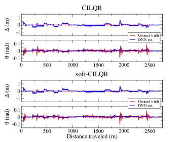
Figure 9: Trajectories obtained for $\Delta$ and $\theta$ by using the CILQR and soft-CILQR controllers under a $\sigma$ value of 0 when the ego vehicle traveled on track A. This experiment corresponds to Exp. V-1 in Table III.

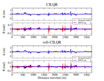
Figure 10: Trajectories obtained for $\Delta$ and $\theta$ by using the CILQR and soft-CILQR controllers under a $\sigma$ value of 0 when the ego vehicle traveled on track B. This experiment corresponds to Exp. V-2 in Table III.

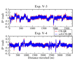
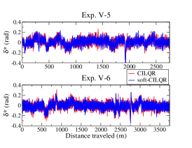
Figure 11: Trajectories obtained for $\delta^{*}$ in Exp. V-1/2, Exp. V-3/4, and Exp. V-5/6 when $\sigma$ = 0, 1, and 2, respectively. The results of the associated quantitative analyses are presented in Table III.

As in the case of the numerical simulations, the vision-based experiments were also performed at various noise levels ($\sigma$ = 0, 1, and 2). The solvers were initialized by setting the control and slack variables to zeros, and the current state was set as follows:

$${\bf x}_{t}=\left[{\begin{array}[]{*{20}c}{\Delta_{D,t}}&0&{\theta_{D,t}}&0\\ \end{array}}\right]^{T}+\sigma{\bf w}_{t},$$ (23)

where $\Delta_{D,t}$ and $\theta_{D,t}$ are current estimations of $\Delta$ and $\theta$, respectively, obtained using the DNN and relevant postprocessing methods [30]. After the optimization process was completed, the first element of the optimal control input sequence ($\delta^{*}$) was entered into the TORCS engine to control the ego vehicle.

The validation results obtained for the CILQR and soft-CILQR solvers on tracks A and B when $\sigma$ = 0 are displayed in Figs. 9 and 10, respectively. In these figures, the DNN-estimated and ground-truth $\Delta$ and $\theta$ data are also shown. When the CILQR and soft-CILQR solvers were used at $\sigma$ values of 1 and 2 (not shown here), the ego vehicle completed the entire range of lane-keeping maneuvers on tracks A and B without leaving the road accidentally. As displayed in Figs. 9 and 10, the maximum distance and angle errors of both solvers on tracks A and B were within 1 m and 0.1 radian, respectively.

The mean absolute errors (MAEs) of $\Delta$ and $\theta$ [30] as well as the root mean square errors (RMSs) of the optimal steering angle $\delta^{*}$ [7] for both solvers are presented in Table III. The MAEs and RMSs can be considered to represent tracking errors and steering smoothness scores, respectively, with lower RMS values for $\delta^{*}$ indicating smoother steering. Standard deviation (SD) [3] can also reflect control performance. As presented in Table III, the CILQR and soft-CILQR controllers exhibited similar performance levels when $\sigma$ = 0. However, as $\sigma$ increased, the influence of disturbances increased, and the ego vehicle controlled using the soft-CILQR controller exhibited smoother steering [Fig. 4(b) and Fig. 5(b)] and lower tracking errors than did that controlled using the CILQR controller. Consequently, the soft-CILQR controller outperformed the CILQR controller on all evaluation metrics when noise existed. The average $\Delta$-MAE, $\theta$-MAE, and $\delta^{*}$-RMS values derived for the soft-CILQR controller were lower than those derived for the CILQR controller by 0.0007 m, 0.0003 rad, and 0.0011 rad, respectively. Fig. 11 presents the $\delta^{*}$ trajectories obtained using the CILQR (red curves) and soft-CILQR (blue curves) controllers. The soft-CILQR controller attenuated the jitter in the steering inputs to a greater extent than did the CILQR controller.

V Conclusions

In this study, we integrated a constraint softening method [13] and the CILQR algorithm [16, 17, 18] to develop a soft-CILQR algorithm for solving the lane-keeping control problem for autonomous vehicles under linear system dynamics. To test and validate the performance of the proposed soft-CILQR algorithm, numerical simulations and vision-based experiments were performed using a path-tracking model [2, 6, 22] under conditions involving additive disturbances. In the numerical simulations, the soft-CILQR algorithm guaranteed the asymptotic convergence of the state trajectories to the target point. The CILQR algorithm also achieved such convergence in the absence of noise ($\sigma$ = 0). However, under conditions involving noise ($\sigma$ = 1 or 2), the soft-CILQR solver generated smoother steering inputs than did the CILQR solver without the use of additional smoothing filters. In the vision-based experiments performed using the experimental setup from our previous work [30], the soft-CILQR algorithm exhibited better performance than did the CILQR algorithm in controlling an autonomous vehicle on TORCS. The soft-CILQR algorithm outperformed the CILQR algorithm in terms of distance ($\Delta$) tracking accuracy, orientation ($\theta$) tracking accuracy, and steering smoothness. The soft-CILQR solver had an efficient computation time of 2.55 ms in the aforementioned experiments. In conclusion, the proposed soft-CILQR algorithm can maintain the stability and safety of autonomous vehicles during lane-keeping tasks under adverse driving conditions.

References

- [1] C. Chen, A. Seff, A. Kornhauser, and J. Xiao, “DeepDriving: Learning affordance for direct perception in autonomous driving,” in Proceedings of the IEEE International Conference on Computer Vision, 2015, pp. 2722-2730.
- [2] D. Li, D. Zhao, Q. Zhang, and Y. Chen, “Reinforcement learning and deep learning based lateral control for autonomous driving,” IEEE Comput. Intell. Mag. vol. 14, no. 2, pp. 83-98, May 2019.
- [3] Y. Wu, S. Liao, X. Liu, Z. Li and R. Lu, “Deep Reinforcement Learning on Autonomous Driving Policy With Auxiliary Critic Network,” IEEE Trans. Neural Netw. Learn. Syst., vol. 34, no. 7, pp. 3680-3690, July 2023.
- [4] J. Wang, H. Sun and C. Zhu, “Vision-Based Autonomous Driving: A Hierarchical Reinforcement Learning Approach,” IEEE Trans. Veh. Technol., vol. 72, no. 9, pp. 11213-11226, Sept 2023.
- [5] A. Savitzky and M. J. Golay, “Smoothing and differentiation of data by simplified least squares procedures,” Anal. Chem., vol. 36, no. 8, pp. 1627–1639, 1964.
- [6] S. Mata, A. Zubizarreta and C. Pinto, “Robust Tube-Based Model Predictive Control for Lateral Path Tracking,” IEEE Trans. Intell. Veh., vol. 4, no. 4, pp. 569-577, Dec 2019.
- [7] E. Chisari, A. Liniger, A. Rupenyan, L. Van Gool and J. Lygeros, “Learning from Simulation, Racing in Reality,” in IEEE International Conference on Robotics and Automation (ICRA), 2021, pp. 8046-8052.
- [8] T. Kim, G. Park, K. Kwak, J. Bae and W. Lee, “Smooth Model Predictive Path Integral Control Without Smoothing,” IEEE Robot. Autom. Lett., vol. 7, no. 4, pp. 10406-10413, Oct 2022.
- [9] A. Zheng and M. Morari, “Stability of model predictive control with mixed constraints,” IEEE Trans. Autom. Control, vol. 40, no. 10, pp. 1818-1823, Oct 1995.
- [10] J. B. Rawlings, “Tutorial overview of model predictive control,” IEEE Control Systems Magazine, vol. 20, no. 3, pp. 38-52, June 2000.
- [11] M. Askari, M. Moghavvemi, H. A. F. Almurib and A. M. A. Haidar, “Stability of Soft-Constrained Finite Horizon Model Predictive Control,” IEEE Trans. Ind. Appl., vol. 53, no. 6, pp. 5883-5892, 2017.
- [12] K. P. Wabersich, R. Krishnadas and M. N. Zeilinger, “A Soft Constrained MPC Formulation Enabling Learning From Trajectories With Constraint Violations,” IEEE Control Syst. Lett., vol. 6, pp. 980-985, 2022.
- [13] S. V. Raković, S. Zhang, H. Sun and Y. Xia, “Model Predictive Control for Linear Systems Under Relaxed Constraints,” IEEE Trans. Autom. Control, vol. 68, no. 1, pp. 369-376, Jan 2023.
- [14] A. G. Wills and W. P. Heath, “Barrier function based model predictive control,” Automatica, vol. 40, pp. 1415-1422, 2004.
- [15] C. Feller and C. Ebenbauer, “Relaxed Logarithmic Barrier Function Based Model Predictive Control of Linear Systems,” IEEE Trans. Autom. Control, vol. 62, no. 3, pp. 1223-1238, March 2017.
- [16] J. Chen, W. Zhan and M. Tomizuka, “Constrained iterative LQR for on-road autonomous driving motion planning,” in IEEE 20th International Conference on Intelligent Transportation Systems (ITSC), 2017, pp. 1-7.
- [17] J. Chen, W. Zhan and M. Tomizuka, “Autonomous Driving Motion Planning With Constrained Iterative LQR,” IEEE Trans. Intell. Veh., vol. 4, no. 2, pp. 244-254, June 2019.
- [18] Y. Shimizu, W. Zhan, L. Sun, J. Chen, S. Kato, and M. Tomizuka, “Motion planning for autonomous driving with extended constrained iterative lqr,” in Dynamic Systems and Control Conference, American Society of Mechanical Engineers, 2020, pp. V001T12A001.
- [19] W. Li and E. Todorov, “Iterative linear quadratic regulator design for nonlinear biological movement systems,” in Proc. 1st Int. Conf. Inform. Control Autom. Robot., 2004, pp. 222–229.
- [20] E. Todorov and W. Li, “A generalized iterative LQG method for locally optimal feedback control of constrained nonlinear stochastic systems,” in Proc. Amer. Control Conf., 2005, pp. 300–306.
- [21] B. Wymann, C. Dimitrakakis, A. Sumner, E. Espié, C. Guionneau, and R. Coulom, “Torcs: the open racing car simulator,” Tech. Rep., 2013.
- [22] K. Lee, S. Jeon, H. Kim and D. Kum, “Optimal Path Tracking Control of Autonomous Vehicle: Adaptive Full-State Linear Quadratic Gaussian (LQG) Control,” IEEE Access, vol. 7, pp. 109120-109133, 2019.
- [23] R. Rajamani, Vehicle Dynamics and Control. Springer, 2011.
- [24] C. Feller and C. Ebenbauer, “Continuous-time linear MPC algorithms based on relaxed logarithmic barrier functions,” in Proc. 19th IFAC World Congr., Cape Town, South Africa, 2014, pp. 2481–2488.
- [25] Y. Tassa, T. Erez and E. Todorov, “Synthesis and stabilization of complex behaviors through online trajectory optimization,” in IEEE/RSJ International Conference on Intelligent Robots and Systems, 2012, pp. 4906-4913.
- [26] Y. Tassa, N. Mansard and E. Todorov, “Control-limited differential dynamic programming,” in IEEE International Conference on Robotics and Automation (ICRA), 2014, pp. 1168-1175.
- [27] J. Hauser and A. Saccon, “A Barrier Function Method for the Optimization of Trajectory Functionals with Constraints,” in Proceedings of the 45th IEEE Conference on Decision and Control, San Diego, CA, USA, 2006, pp. 864-869.
- [28] C. Feller and C. Ebenbauer, “A stabilizing iteration scheme for model predictive control based on relaxed barrier functions,” Automatica, vol. 80, pp. 328-339, June 2017.
- [29] B. Kouvaritakis, and M. Cannon, Model Predictive Control. Springer Press, 2016.
- [30] D.-H. Lee, “Efficient Perception, Planning, and Control Algorithms for Vision-Based Automated Vehicles”, 2022, arXiv:2209.07042. [Online]. Available: https://arxiv.org/abs/2209.07042
- [31] O. Ronneberger, P. Fischer, and T. Brox, “U-Net: Convolutional networks for biomedical image segmentation,” in International Conference on Medical Image Computing and Computer-Assisted Intervention (MICCAI), Springer, 2015, pp. 234-241.
- [32] C. V. Samak, T. V. Samak, and S. Kandhasamy, “Control Strategies for Autonomous Vehicles,” 2021, arXiv:2011.08729. [Online]. Available: https://arxiv.org/abs/2011.08729