Imputation using training labels and classification via label imputation

Abstract

Missing data is a common problem in practical data science settings. Various imputation methods have been developed to deal with missing data. However, even though in many situations, the labels are available in the training data, the common practice of imputation usually only relies on the input and ignores the label. We propose imputation using labels (IUL) algorithm, a strategy that stacks the label into the input and illustrate how it can significantly improve the imputation quality of the input. In addition, we propose Classification Based on MissForest Imputation (CBMI) a classification strategy that initializes the predicted test label with missing values and stacks the label with the input for imputation, and the imputation is based on the well-know MissForest algorithm [1]. This allows imputing the label and the input at the same time. Also, the technique is capable of handling data training with missing labels without any prior imputation and is applicable to continuous, categorical, or mixed-type data. Experiments suggest promising improvement in terms of mean squared error/classification accuracy, especially for imbalanced data, categorical data and small sample data. Importantly, the experiment results suggest that when a dataset has too little sample to build a good classification model upon, merging the training and testing data and imputing the label as CBMI can be a significantly better option.

I Introduction

Data can come in various forms, ranging from continuous numerical values to discrete values and mixed between categorical and continuous. For example, a dataset on housing may contain information about the price, and areas, which are continuous, while the number of rooms and number of bathrooms are discrete features. In addition, it is also common to encounter missing data. This can happen for various reasons, such as malfunctioning devices, broken sensors, or people declining to fill in survey information, etc. This can undermine the integrity and robustness of analyses, potentially leading to biased results and incomplete insights. Consequently, the need for methodologies to address missing data becomes paramount, prompting the widespread adoption of imputation techniques.

Imputation, as a remedial practice, involves the estimation or prediction of missing values based on observed information. This process becomes particularly intricate when dealing with datasets that encompass diverse data types, including continuous, categorical, and mixed data. In response to this complexity, a spectrum of imputation techniques has been developed, each tailored to handle specific data types and patterns [2, 1]. In addition, in recent years, classification or regression models that can handle missing data directly such as Decision Tree Classifier [3], LSTM [4] have also captured a lot of attention. However, imputation remained a popular choice as it renders the data complete not only for the classification or regression task but also data visualization or other inferences.

In this work, we propose stacking training labels to training input to improve the imputation of the training input and illustrate how this can significantly improve the imputation of training input. Moreover, we propose Classification Based on MissForest Imputation (CBMI) to predict the label on testing data without building a classification model on the training set. The method starts by initializing the predicted testing labels with missing values. Then, it stacks the input and the label, the training and testing data together, and uses missForest algorithm [1] to impute all the missing values in the matrix. The imputation returns a matrix that contains imputed training and testing input, imputed training labels if the training labels contain missing data, and predicted testing labels.

Our contribution are as following: (i) We propose using training labels to aid the imputation of the training input and illustrate how this can significantly improve the imputation of training input; (ii) We propose CBMI algorithm for predicting the output of a classification task via imputation, instead of building a model on training data and then predicting on a test set; (ii) we conduct various experiments to illustrate that most of the time, the proposed approaches provide better accuracy for classification.

The rest of this paper is organized as follows: In section II, we detail some related works in this area. Next, in section III, we review the fundamentals of the MissForest algorithm [1]. Then, in section IV, we detail our proposed methods. Finally, we conducts the experiments to illustrate the power of the proposed techniques in section V and summarize the main ideas of the paper in section VI.

II Related works

A diverse array of techniques, ranging from traditional methods to sophisticated algorithms, has been developed to handle missing data. Each method brings unique strengths, making them suitable for different types of data and analysis scenarios. Traditional approaches, for example, complete case analysis, have been widely used due to their simplicity but are prone to bias due to the exclusion of observations with missing values. More sophisticated methods, such as multiple imputation [5] or multiple imputation using Deep Denoising Autoencoders [6], have emerged to mitigate these challenges. The methods acknowledge the uncertainty associated with the imputation process by generating multiple plausible values for each missing data point. Another notable work is the Conditional Distribution-based Imputation of Missing Values (DIMV) [2] algorithm. The algorithm finds the conditional distribution of features with missing values based on fully observed features, and its imputation step provides coefficients with direct explainability similar to regression coefficients.

Regression and clustering-based methods also play a significant role in addressing missing data. The CBRL and CBRC algorithms [7], utilizing Bayesian Ridge Regression, showcase the efficacy of regression-based imputation methods. Additionally, the cluster-based local least square method [8] offers an alternative approach to imputation based on clustering techniques. For big datasets, deep learning imputation techniques are also of great use due to their powerful performance [9, 10, 11].

For continuous data, techniques based on matrix decomposition or matrix completion, such as Polynomial Matrix Completion [12], Alternating Least Squares (ALS) [13], and Nuclear Norm Minimization [14], have been employed to make continuous data complete, enabling subsequent analysis using regular data analysis procedures. For categorical data, various techniques have been explored. The use of k-Nearest Neighbors imputation involves identifying missing values, selecting neighbors based on a similarity metric (e.g., Hamming distance), and imputing missing values by a majority vote from the neighbors’ known values. Moreover, the missForest imputation method [1] has shown efficacy in handling datasets that comprise a mix of continuous and categorical features. In addition, some other methods that can handle mixed data include FEMI [15], SICE [16], and HCMM-LD [17].

In recent years, there has been a notable shift towards the development of classification methods and models capable of directly handling missing data, circumventing the need for imputation. These approaches recognize that imputation introduces a layer of uncertainty and potential bias and instead integrates mechanisms to utilize the available information effectively. Typically tree-based methods that have such capabilities are Gradient-boosted trees [18], Decision Tree Classifier [3], and their implementation are readily available in the sklearn package [19].

The Random Forest classifier has been a pivotal contribution in the field of machine learning, renowned for its robustness and versatility. Originating from ensemble learning principles, Random Forests combine the predictions of multiple decision trees to enhance overall predictive accuracy and mitigate overfitting. This approach was introduced by Breiman in 2001 [20], and since then, it has gained widespread adoption across diverse domains. The classifier’s ability to handle high-dimensional data, capture complex relationships, and provide estimates of feature importance has made it particularly valuable. Various extensions and modifications to the original Random Forest algorithm have been proposed to address specific challenges. For instance, methods like Extremely Randomized Trees [21] introduce additional randomness during the tree-building process, contributing to increased diversity and potentially improved generalization. Additionally, research efforts have explored adapting Random Forests for specialized tasks, such as imbalanced classification, time-series analysis, and feature selection.

III Preliminary: missForest algorithm

MissForest [1] is an imputation algorithm used for handling missing data in datasets. It is suitable not only for continuous or categorical but also for mixed-type data. The algorithm works by iteratively constructing a random forest based on the observed data, and then using this forest to predict missing values in the dataset. The process is repeated until convergence, refining the imputations in each iteration. MissForest is advantageous for its ability to handle non-linear relationships and interactions in the data, making it suitable for a wide range of applications. In addition, one key feature of MissForest is its adaptability to various types of missing data patterns, such as missing completely at random (MCAR), missing at random (MAR), and missing not at random (MNAR). This flexibility makes it a versatile tool for imputing missing values in datasets with complex structures.

Algorithm 1 MissForest algorithm

Input:

1. a matrix $\mathbf{X}\in\mathbb{R}^{n\times p}$,

2. stopping criteron $\gamma$

Procedure:

1:initialize missing values in $\mathbf{X}$ by some imputation method

2:$\mathbf{k}\leftarrow$ sorted indices of features in $\mathbf{X}$ in an increasing order of missing values

3:while not $\gamma$ do:

4:     $\mathbf{X}_{old}^{imp}\leftarrow$ previously imputed version of $\mathbf{X}$,

5:     for $s$ in $\mathbf{k}$ do:

6:         fit a random forest where the observed values in $\mathbf{X}_{s}$ is the response, and the corresponding values of features in $\mathbf{X}$ other than $\mathbf{X}_{s}$ as the input

7:         predict $\mathbf{y}_{miss}^{(s)}$ (the missing values in $\mathbf{X}_{s}$) based on the features other $\mathbf{X}_{s}$.

8:         $\mathbf{X}_{new}^{imp}\leftarrow$ updated version of $\mathbf{X}$ using $\mathbf{y}_{miss}^{(s)}$

9:     end for

10:     Update $\gamma$.

11:end while

Return: the imputed version of $\mathbf{X}$.

For the setting of the proposed CBMI method, we use the default missForest setting for $\gamma$. That means that, a set of continuous features $F$, $\gamma$ is governed by

$$\Delta=\frac{\sum_{j\in F}(\mathbf{X}_{new}^{imp}-\mathbf{X}_{old}^{imp})^{2}}{\sum_{j\in F}(\mathbf{X}_{new}^{imp})^{2}},$$ (1)

while for a set of categorical features $G$, $\gamma$ is governed by

$$\Delta_{G}=\frac{\sum_{j\in G}\sum_{i=1}^{n}\mathbf{I}_{\mathbf{X}_{new}^{imp}\neq\mathbf{X}_{old}^{imp}}}{\#NA}.$$ (2)

Here, $\#NA$ is the number of missing entries in the categorical features.

IV Methodology

IV-A Using labels for imputation

In this section, we detail the idea of imputation using labels (IUL). For clarity, from now, we refer to the common imputation procedure that only relies on the input itself, without the labels, as direct imputation (DI).

The IUL process is straightforward and presented in algorithm 2. Suppose that we have input data $\mathbf{X}_{train}$ and labels $\mathbf{y}_{train}$. Then, the procedure starts by stacking the input training data $\mathbf{X}_{train}$ and labels $\mathbf{y}_{train}$ in a column-wise manner in step 1. Then, in step 2, the algorithm uses the imputation method $I$ to impute $\mathcal{D}_{train}$. This gives $\mathcal{D}_{train}^{imp}$. Then in step 3, the algorithm assigns $\mathbf{X}_{train}^{imp}$, the imputed version of $\mathbf{X}_{train}$, to be the submatrix of $\mathcal{D}_{train}$ that consists of all columns except the last column of $\mathcal{D}_{train}$. In addition in step 4, the algorithm assigns $\mathbf{y}_{train}^{imp}$, the imputed version of $\mathbf{y}_{train}$ (if $\mathbf{y}_{train}$ contains missing values), to be the last column of $\mathcal{D}_{train}^{imp}$. The algorithm ends by returning $\mathbf{X}_{train}^{imp},\mathbf{y}_{train}^{imp}$.

Algorithm 2 IUL algorithm

Input:

1. input training data $\mathbf{X}_{train}$, labels $\mathbf{y}_{train}$

2. imputation algorithm $I$.

Procedure:

1:$\mathcal{D}_{train}=[\mathbf{X}_{train}|\mathbf{y}_{train}]$

2:$\mathcal{D}_{train}^{imp}\leftarrow$ the imputed version of $\mathcal{D}_{train}$ using the imputation algorithm $I$.

3:$\mathbf{X}_{train}^{imp}\leftarrow$ imputed version of $\mathbf{X}_{train}$ that consists of all columns except the last column of $\mathcal{D}_{train}$,

4:$\mathbf{y}_{train}^{imp}\leftarrow$ imputed version of $\mathbf{y}_{train}$ if $\mathbf{y}_{train}$ contains missing values. This corresponds to the last column of $\mathcal{D}_{train}^{imp}$.

Return: $\mathbf{X}_{train}^{imp},\mathbf{y}_{train}^{imp}$

IV-A1 Remarks

It is important to note that the IUL algorithm can handle not only $\mathbf{X}_{train}$ with missing data, but also $\mathbf{y}_{train}$ with missing data. In case the labels contain missing data, the returned $\mathbf{y}_{train}^{imp}$ is the imputed version of the training labels. So, this also has a great potential to be applied to semi-supervised learning, as in such a setting, the samples without labels can be considered as samples with missing labels.

It is also important to notice that IUL can be used with other imputation techniques than MissForest. However, due to the limited space, in this study, we only examine the performance of MissForest.

Next, note that the difference in the number of choices for building a random forest when stacking the label to the input as in IUL can be significantly higher than imputing based only on $\mathbf{X}_{train}$ itself. To be more specific, assuming we have $p$ features in $\mathbf{X}_{train}$ and one label $\mathbf{y}$. With IUL, the label can be utilized to aid the imputation of $\mathbf{X}_{train}$, which means that we have $p+1$ features. In particular, if we are to build $m$ model RandomForest and choose $k$ features for each model then we can have $\begin{pmatrix}p+1\\ k\end{pmatrix}$ combinations. Meanwhile, DI only work on $\mathbf{X}_{train}$ so there are just $\begin{pmatrix}p\\ k\end{pmatrix}$ options. The difference is

$$\begin{pmatrix}p+1\\ k\end{pmatrix}-\begin{pmatrix}p\\ k\end{pmatrix}=\begin{pmatrix}p\\ k-1\end{pmatrix},$$ (3)

which can be extremely large.

IV-B Classification via imputation

In this section, we detail the methodology of the proposed Classification Based on MissForest Imputation (CBMI) method. The algorithm is presented in algorithm 3.

Suppose that we have a dataset that consists of the training set $\{\mathbf{X}_{train},\mathbf{y}_{train}\}$ that has $n_{train}$ samples and the testing set $\{\mathbf{X}_{test},\mathbf{y}_{test}\}$ that has $n_{test}$ samples. Then, the procedure is as follows:

At the first step of the algorithm, we stack the training input $\mathbf{X}_{train}$ and the training label $\mathbf{y}_{train}$ in a column-wise manner. Next, in step 2, we initiate the predicted label of the test set $\hat{\mathbf{y}}$ with missing values, denoted by $*$. After that, in step 3, we stack the input of the test set $\mathbf{X}_{test}$ and $\hat{\mathbf{y}}$ in a column-wise manner, and we call this $\mathcal{D}_{test}^{*}$.

In the fourth step, we stack $\mathcal{D}_{train}$ and $\mathcal{D}_{test}^{*}$ in a row-wise manner. This gives us $\mathcal{D}^{*}$. Then, at step 5, we impute $\mathcal{D}^{*}$ using the MissForest algorithm. This gives us an imputed matrix $\mathcal{D}$ that contains the imputed training, testing input, and the imputed label of the training set if the training data has missing labels and the imputed label $\hat{\mathbf{y}}$ of the test set.

Algorithm 3 CBMI algorithm

Input:

1. a dataset consists of the training set $\{\mathbf{X}_{train},\mathbf{y}_{train}\}$ that has $n_{train}$ samples and the testing set $\{\mathbf{X}_{test},\mathbf{y}_{test}\}$ that has $n_{test}$ samples,

Procedure:

1:$\mathcal{D}_{train}=[\mathbf{X}_{train}|\mathbf{y}_{train}]$

2:$\hat{\mathbf{y}}=\begin{pmatrix}*\\ \vdots\\ *\end{pmatrix}$: an NA-initiated vector of size $n_{test}$ where ${n_{test}}$ is the number of sample in the test set

3:$\mathcal{D}_{test}^{*}=[\mathbf{X}_{test}|\hat{\mathbf{y}}]$

4:$\mathcal{D}^{*}=\begin{pmatrix}\mathcal{D}_{train}\\ \mathcal{D}_{test}^{*}\end{pmatrix}$

5:$\mathcal{D}\leftarrow$ the imputed version of $\mathcal{D}^{*}$ using the missForest algorithm

Return: $\mathcal{D}$, the imputed version of $\hat{\mathbf{y}}$ obtained from $\mathcal{D}$.

So, instead of following the conventional way of imputing the data and then build a model on training set, CBMI conducts no prior imputation and build no model on training data to predict the label of the test set. Instead, CBMI combine the training and testing data, including the input and the available and NA-initialized labels together to impute the label of the test set.

V Experiments

V-A Experiment set up

We compare the imputation using labels (IUL) with the direct imputation on training data approach (DI) by splitting a dataset into training and testing sets with a ratio of 6:4 and simulating missing rates $20\%-80\%$ on the training input. Here, the missing rate is defined as the ratio between the number of missing entries and the total number of entries. After missing data generation, the data is scaled to $[-1,1]$. Each experiment is repeated 10 times, and we report the mean and standard deviation of accuracy and running time. We use MissForest as the imputation method with default configuration and Random Forest as the classifier.

In addition, we compare CBMI with the two-step approach of Imputation using missForest and then Classification using Random Forest Classifier [20], abbreviated as IClf. The reason for choosing Random Forest as the Classifier is to facilitate fair comparison with CBMI, which relies on Random Forest to impute missing values. The stopping criterion for missForest is the default in the missingpy package .

The datasets for the experiments are from the UCI Machine Learning repository [22], and are described in table I. For each dataset, we simulate missing data with missing rates $r$ ranging between 0% - 80%. Each experiment is repeated 10 times, and the training-to-testing ratio is 6:4, and we report the mean $\pm$ standard deviation from the runs for both the accuracy and the running time. We also conducted the experiments in two settings: the test set is fully observed and the test set has missing values. In case the test set is fully observed, the missing rate $r$ is the missing rate for simulating missing values on training data only. In the case where there are missing values in the dataset, the missing values are generated with the same missing rates as in the training input.

For a fair comparison, for IClf, if the test set contains missing data then it is merged with the train set for imputation. Note that this is only for the imputation of the test set only. The imputation of the training data is independent of the testing data. The codes for this paper will be made available upon the acceptance.

TABLE I: Datasets for experiments

Datasets	# samples	# features
Iris	150	4
liver	345	6
soybean	47	35
Parkinson	195	22
heart	267	44
glass	214	9
car	1728	6

V-B Results and Analysis for IUL

The results of the experiments on the performance of IUL are shown in figures 2, 3, 4, 5. Note that the soybean dataset and the car dataset contain solely categorical features. Therefore, the MSE plot for that dataset is not available. From the figures, we can see that while in some cases, IUL and DI have similar performance, a clear improvement of IUL compared to DI can be seen in the glass dataset (figure 5) and the Iris dataset (figure 1).

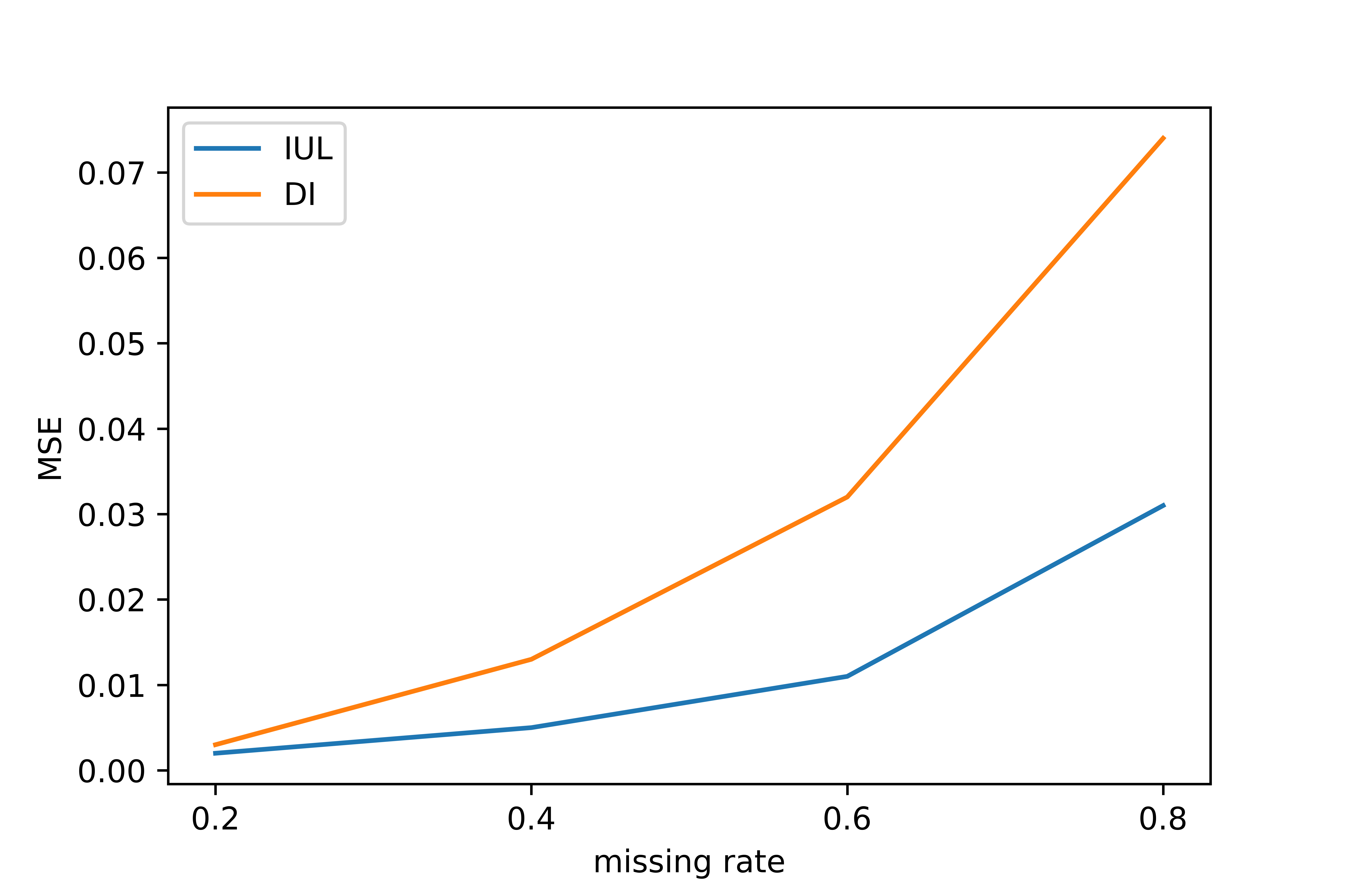
Figure 1: MSE of IUL and DI on the Iris dataset.

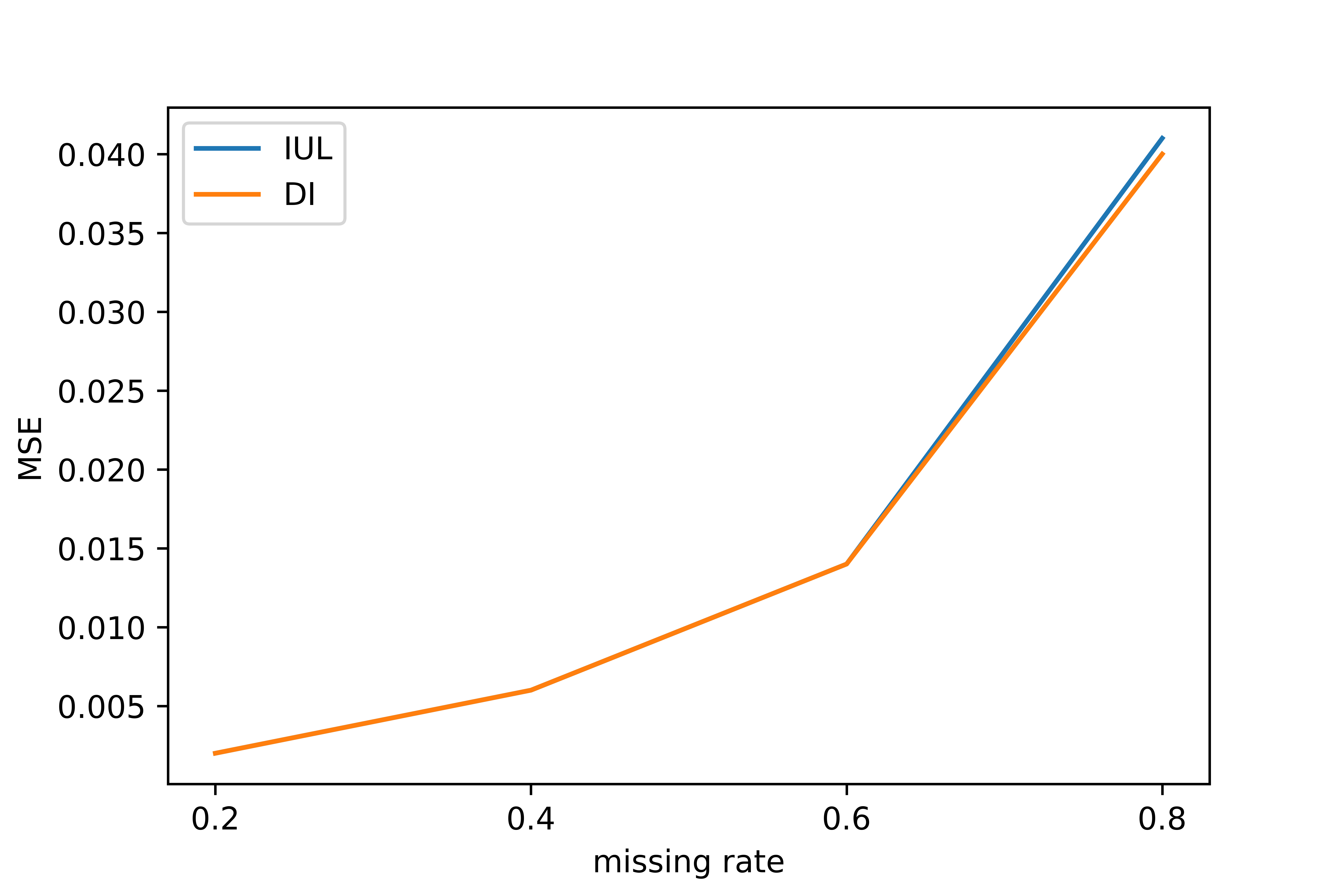
Figure 2: MSE of IUL and DI on the heart dataset.

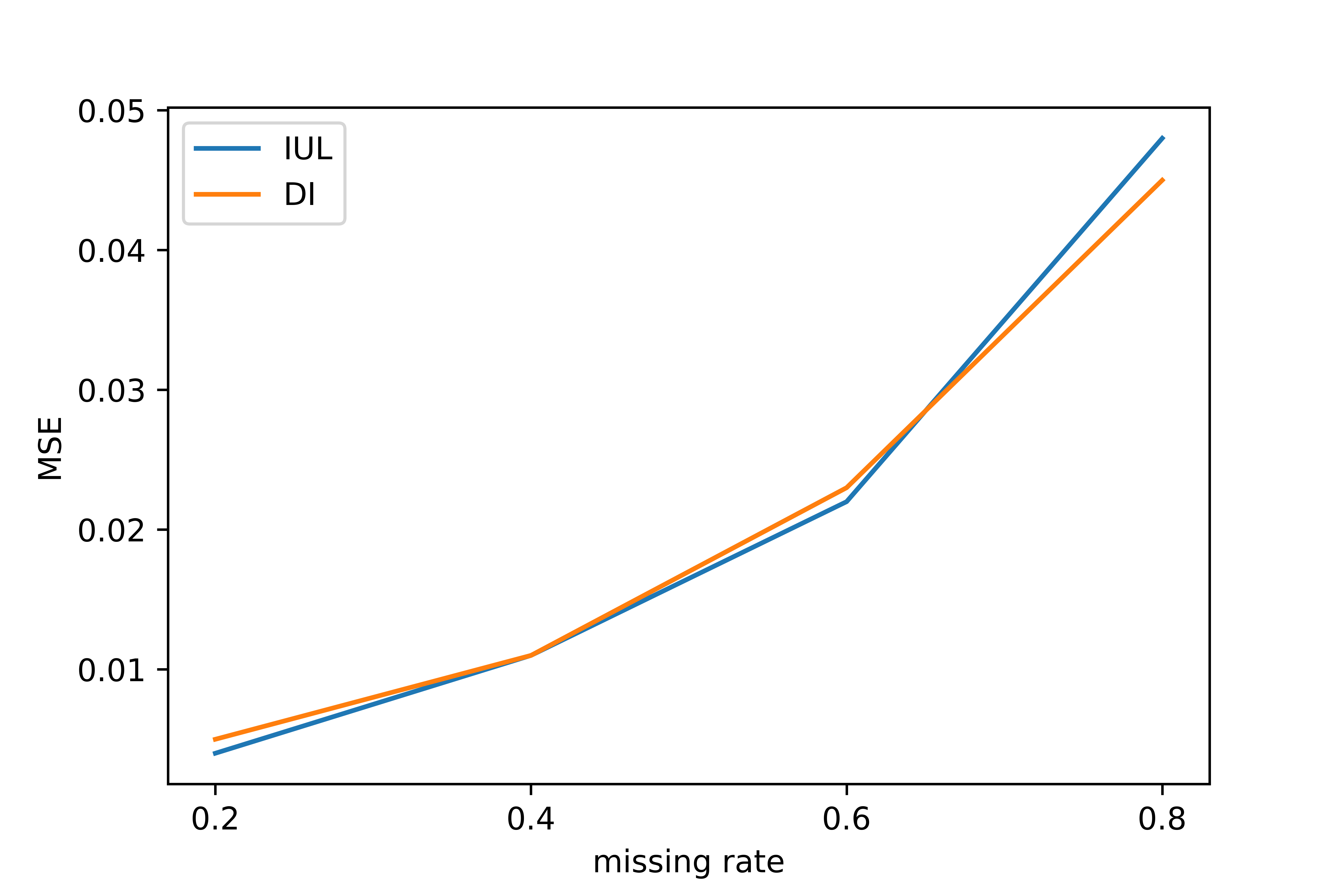
Figure 3: MSE of IUL and DI on the liver dataset.

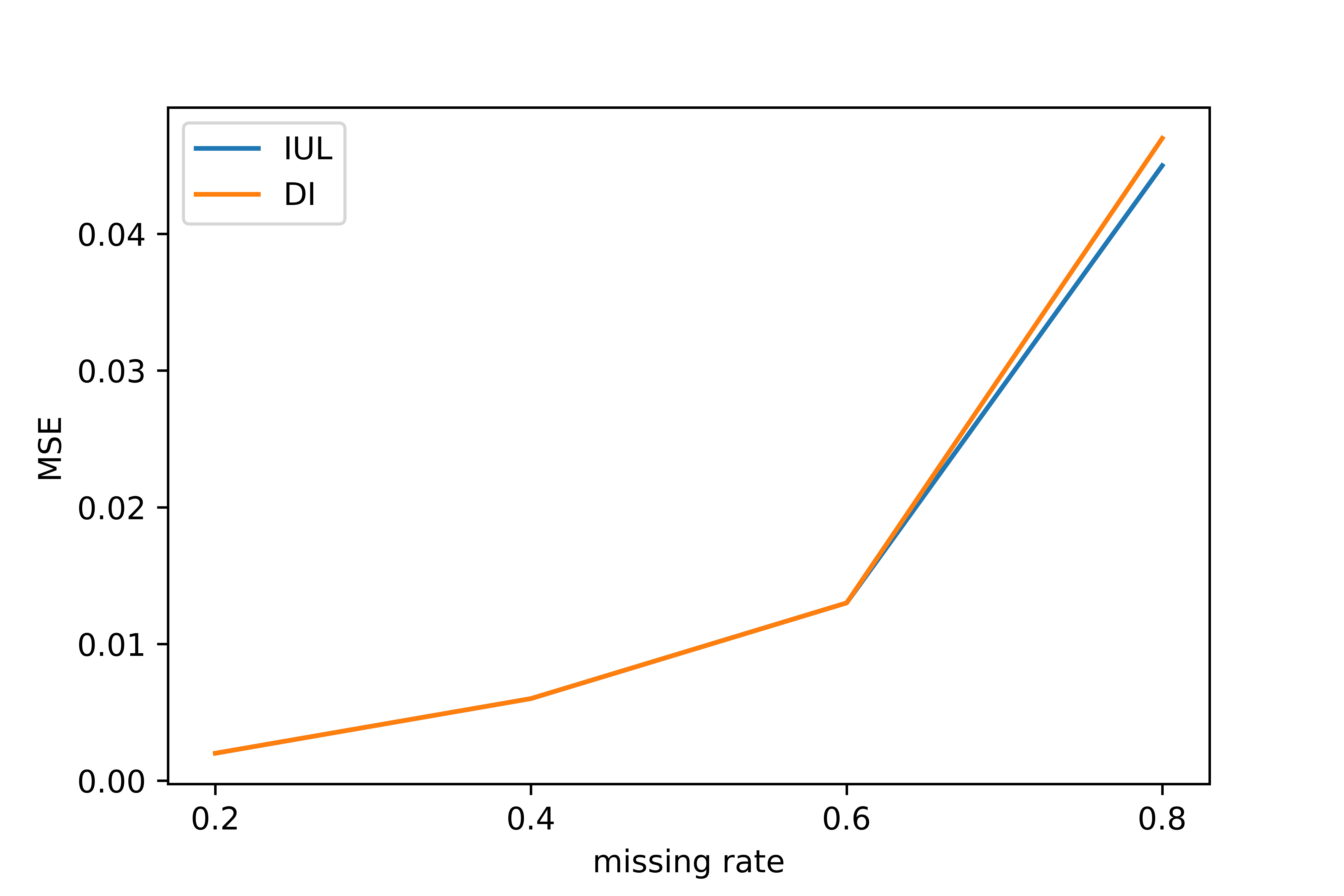
Figure 4: MSE of IUL and DI on the parkinson dataset.

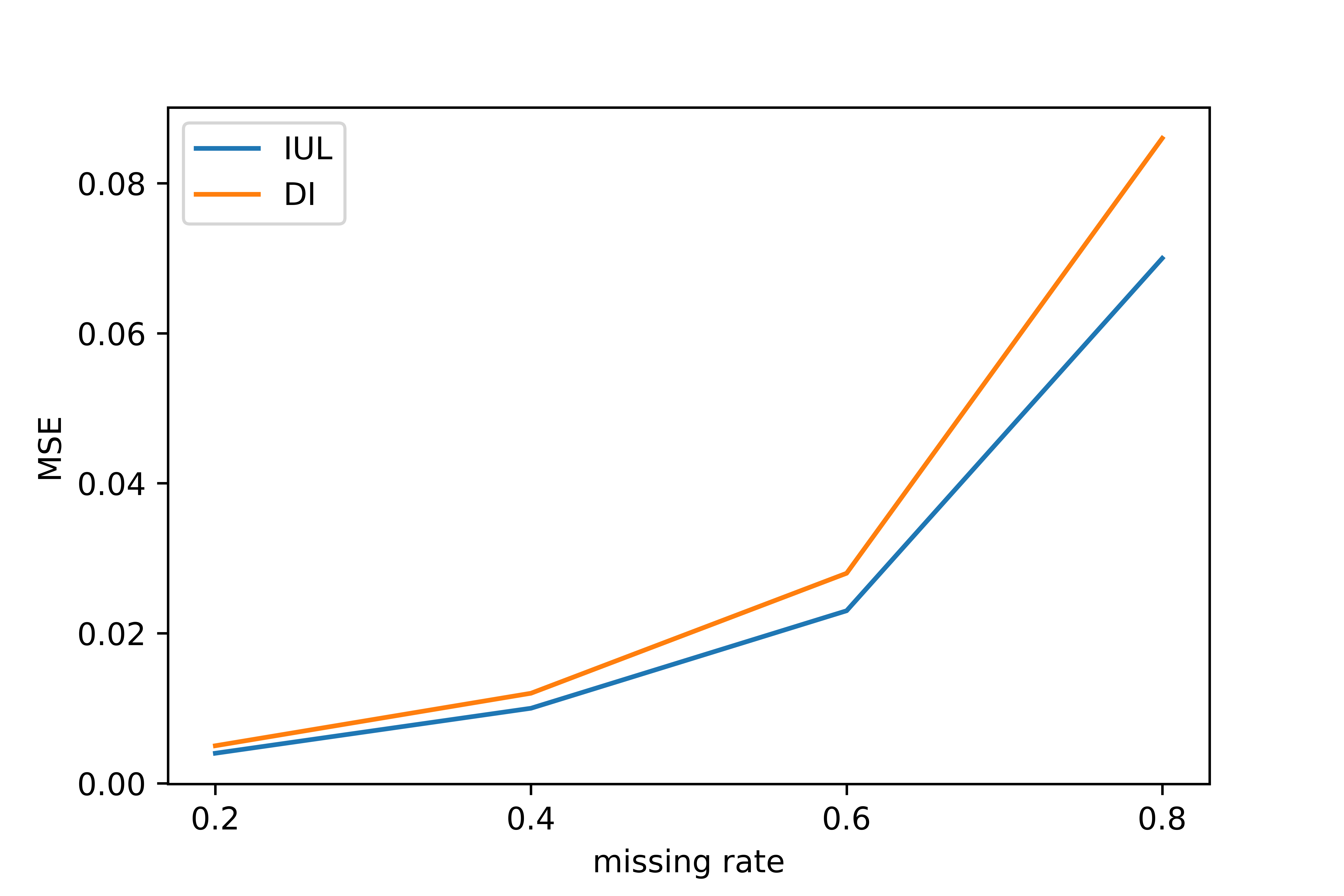
Figure 5: MSE of IUL and DI on the glass dataset.

V-C Results and Analysis for CBMI

The results for the experiments on the performance of IUL are shown in Table III, IV, V, VI, X, XI, XII, XIII.

From these tables, we see that most of the time, CBMI achieves better results than IClf. For example, at missing rate $r=80\%$, for the soybean dataset when missing data present in the test set (table IV), the accuracy of CBMI is $0.547$, while it is $0.5$ for IClf. This implies a significant improvement of $4.7\%$ when using CBMI compared to IClf. In addition, most of the time, the standard deviation of the accuracy obtained from CBMI is also smaller than IClf.

Interestingly, CBMI achieves better results than IClf for many cases where the missing rate $r$ is zero, i.e., there is no missing data in the training set. For example, when the training dataset is fully observed ($r=0$) on the heart dataset with missing data present in the test set (table VI), CBMI gives an accuracy of $0.821$, while IClf gives $0.817$; or on the glass dataset where the test set is fully observed (table (table XIV), CBMI’s accuracy is $0.762$, while IClf’s accuracy is $0.751$. Note that such an improvement is small but in many applications such as healthcare or banking, such a small improvement is still significant. In addition, these comparisons show that even for a dataset without missing data, CBMI may provide better test accuracy than building a Random Forest classification model on training data and predict the labels of the test set.

Regarding the running time, when missing data present in the test set, from tables III, IV, V and VI, we can see that when missing data presents in the test set, CBMI is clearly faster. However, from tables X, XI, XII, XIII, when the testing data is fully observed, IClf is slightly faster than CBMI most of the time. This is possibly because when the testing data is fully observed, the CBMI’s imputation process has to impute a larger matrix, which consists of the training and testing input and labels, while IClf imputes only the training input.

TABLE II: Classification results on the Iris dataset when missing data presents in the test set

	accuracy		running time
missing rate	CBMI	IClf	CBMI	IClf
20 %	0.922$\pm$0.045	0.935$\pm$0.026	3.165$\pm$0.87	4.346$\pm$0.79
40 %	0.873$\pm$0.032	0.873$\pm$0.047	3.57$\pm$0.61	5.312$\pm$1.079
60 %	0.752$\pm$0.065	0.75$\pm$0.049	3.234$\pm$0.769	4.875$\pm$0.497
80 %	0.583$\pm$0.064	0.585$\pm$0.035	3.389$\pm$1.158	4.172$\pm$0.955

TABLE III: Classification results on the liver dataset when missing data presents in the test set

	accuracy		running time
$r$	CBMI (our)	IClf	CBMI (our)	IClf
20 %	0.649$\pm$0.022	0.642$\pm$0.019	5.379$\pm$1.778	7.094$\pm$1.237
40 %	0.587$\pm$0.046	0.583$\pm$0.028	5.658$\pm$1.421	7.662$\pm$1.659
60 %	0.541$\pm$0.041	0.562$\pm$0.042	5.715$\pm$1.594	7.502$\pm$1.428
80 %	0.554$\pm$0.025	0.547$\pm$0.048	5.704$\pm$1.685	7.774$\pm$1.775

TABLE IV: Classification results on the soybean dataset when missing data presents in the test set

	accuracy		running time
$r$	CBMI (our)	IClf	CBMI (our)	IClf
20 %	0.989$\pm$0.021	0.984$\pm$0.034	24.579$\pm$5.383	45.279$\pm$6.573
40 %	0.916$\pm$0.116	0.9$\pm$0.106	27.251$\pm$6.12	44.467$\pm$5.554
60 %	0.821$\pm$0.092	0.8$\pm$0.091	29.487$\pm$5.299	44.25$\pm$9.486
80 %	0.547$\pm$0.142	0.5$\pm$0.127	26.82$\pm$6.247	48.91$\pm$8.085

TABLE V: Classification results on the Parkinson dataset when missing data presents in the test set

	accuracy		running time
$r$	CBMI (our)	IClf	CBMI (our)	IClf
20 %	0.877$\pm$0.024	0.869$\pm$0.038	15.456$\pm$4.69	27.058$\pm$5.667
40 %	0.862$\pm$0.045	0.858$\pm$0.043	18.927$\pm$3.824	26.745$\pm$2.528
60 %	0.795$\pm$0.035	0.813$\pm$0.039	18.949$\pm$4.077	22.418$\pm$5.805
80 %	0.778$\pm$0.037	0.769$\pm$0.06	18.711$\pm$4.516	27.507$\pm$5.776

TABLE VI: Classification results on the heart dataset when missing data presents in the test set

	accuracy		running time
$r$	CBMI (our)	IClf	CBMI (our)	IClf
20 %	0.83$\pm$0.038	0.83$\pm$0.036	42.814$\pm$8.138	74.018$\pm$12.008
40 %	0.809$\pm$0.048	0.813$\pm$0.037	50.46$\pm$5.902	87.255$\pm$11.24
60 %	0.806$\pm$0.025	0.801$\pm$0.029	47.827$\pm$5.954	86.801$\pm$9.228
80 %	0.779$\pm$0.036	0.783$\pm$0.05	48.81$\pm$4.614	90.821$\pm$7.51

TABLE VII: Classification results on the glass dataset when missing data presents in the test set

	accuracy		running time
$r$	CBMI (our)	IClf	CBMI (our)	IClf
20 %	0.705$\pm$0.036	0.692$\pm$0.052	8.161$\pm$1.42	11.92$\pm$1.64
40 %	0.633$\pm$0.048	0.598$\pm$0.074	9.097$\pm$2.013	12.305$\pm$1.235
60 %	0.527$\pm$0.039	0.535$\pm$0.031	6.633$\pm$1.839	12.21$\pm$1.989
80 %	0.422$\pm$0.049	0.35$\pm$0.055	9.734$\pm$2.092	11.475$\pm$2.754

TABLE VIII: Classification results on the car dataset when missing data presents in the test set

	accuracy		running time
$r$	CBMI (our)	IClf	CBMI (our)	IClf
20 %	0.768$\pm$0.012	0.758$\pm$0.012	6.278$\pm$1.198	11.405$\pm$1.771
40 %	0.707$\pm$0.019	0.694$\pm$0.020	6.564$\pm$1.147	11.673$\pm$1.593
60 %	0.678$\pm$0.020	0.670$\pm$0.040	6.450$\pm$1.160	11.846$\pm$2.382
80 %	0.682$\pm$0.015	0.678$\pm$0.015	5.835$\pm$1.524	9.369$\pm$1.681

TABLE IX: Classification results on the Iris dataset when the test input is fully observed

	accuracy		running time
$r$	CBMI (our)	IClf	CBMI (our)	IClf
0 %	0.955$\pm$0.024	0.953$\pm$0.023	0.350$\pm$0.013	0.083$\pm$0.001
20 %	0.963$\pm$0.024	0.952$\pm$0.028	3.911$\pm$1.039	2.755$\pm$0.632
40 %	0.945$\pm$0.020	0.943$\pm$0.015	3.576$\pm$0.913	2.483$\pm$0.510
60 %	0.943$\pm$0.020	0.917$\pm$0.041	3.376$\pm$0.872	2.423$\pm$0.653
80 %	0.948$\pm$0.020	0.798$\pm$0.108	2.810$\pm$0.707	1.964$\pm$0.792

TABLE X: Classification results on the liver dataset when the test input is fully observed

	accuracy		running time
$r$	CBMI (our)	IClf	CBMI (our)	IClf
0 %	0.707$\pm$0.029	0.712$\pm$0.035	0.395$\pm$0.002	0.095$\pm$0.002
20 %	0.687$\pm$0.032	0.67$\pm$0.015	5.898$\pm$1.426	3.664$\pm$0.886
40 %	0.664$\pm$0.037	0.624$\pm$0.037	5.209$\pm$2.157	4.223$\pm$0.565
60 %	0.646$\pm$0.056	0.632$\pm$0.049	6.262$\pm$1.813	4.115$\pm$1.322
80 %	0.568$\pm$0.033	0.565$\pm$0.046	6.162$\pm$1.465	2.558$\pm$1.065

TABLE XI: Classification results on the soybean dataset when the test input is fully observed. Missing rate 80% gives some samples that are completely empty. So we discard this case.

	accuracy		running time
$r$	CBMI (our)	IClf	CBMI (our)	IClf
0 %	0.995$\pm$0.016	1.0$\pm$0.0	0.709$\pm$0.052	0.116$\pm$0.014
20 %	0.995$\pm$0.016	0.995$\pm$0.016	57.483$\pm$14.496	63.033$\pm$8.178
40 %	0.989$\pm$0.021	0.963$\pm$0.062	50.181$\pm$15.803	43.733$\pm$9.249
60 %	0.995$\pm$0.016	0.937$\pm$0.061	27.561$\pm$11.688	25.348$\pm$9.366

TABLE XII: Classification results on the parkinson dataset when the test input is fully observed

	accuracy		running time
$r$	CBMI (our)	IClf	CBMI (our)	IClf
0 %	0.904$\pm$0.037	0.895$\pm$0.045	0.368$\pm$0.006	0.092$\pm$0.003
20 %	0.863$\pm$0.041	0.871$\pm$0.05	16.72$\pm$3.905	15.741$\pm$4.267
40 %	0.865$\pm$0.026	0.862$\pm$0.033	18.888$\pm$4.622	13.52$\pm$1.636
60 %	0.873$\pm$0.032	0.847$\pm$0.045	16.582$\pm$5.786	10.715$\pm$3.629
80 %	0.79$\pm$0.071	0.799$\pm$0.05	19.093$\pm$5.147	13.792$\pm$5.38

TABLE XIII: Classification results on the heart dataset when the test input is fully observed

	accuracy		running time
$r$	CBMI (our)	IClf	CBMI (our)	IClf
0 %	0.82$\pm$0.017	0.818$\pm$0.023	0.375$\pm$0.004	0.101$\pm$0.001
20 %	0.813$\pm$0.04	0.808$\pm$0.039	38.631$\pm$8.816	35.641$\pm$5.884
40 %	0.819$\pm$0.031	0.815$\pm$0.039	46.706$\pm$9.855	41.273$\pm$6.889
60 %	0.825$\pm$0.032	0.811$\pm$0.032	44.298$\pm$8.777	42.332$\pm$8.138
80 %	0.777$\pm$0.04	0.78$\pm$0.038	45.646$\pm$7.224	37.522$\pm$7.628

TABLE XIV: Classification results on the glass dataset when the test input is fully observed

	accuracy		running time
$r$	CBMI (our)	IClf	CBMI (our)	IClf
0 %	0.762$\pm$0.055	0.751$\pm$0.063	0.377$\pm$0.003	0.092$\pm$0.001
20 %	0.763$\pm$0.049	0.745$\pm$0.048	7.41$\pm$1.166	5.791$\pm$1.228
40 %	0.738$\pm$0.022	0.701$\pm$0.035	8.132$\pm$2.086	5.787$\pm$1.558
60 %	0.669$\pm$0.068	0.629$\pm$0.039	7.655$\pm$1.919	5.266$\pm$1.384
80 %	0.588$\pm$0.075	0.503$\pm$0.027	8.056$\pm$2.292	5.662$\pm$1.476

TABLE XV: Classification results on the car dataset when the test input is fully observed

	accuracy		running time
$r$	CBMI (our)	IClf	CBMI (our)	IClf
0 %	0.962$\pm$0.009	0.959$\pm$0.012	0.431$\pm$0.012	0.112$\pm$0.001
20 %	0.892$\pm$0.01	0.867$\pm$0.018	7.202$\pm$0.988	6.009$\pm$1.498
40 %	0.828$\pm$0.023	0.793$\pm$0.02	7.282$\pm$1.258	5.476$\pm$0.675
60 %	0.79$\pm$0.018	0.73$\pm$0.01	6.557$\pm$1.273	5.759$\pm$1.34
80 %	0.72$\pm$0.035	0.716$\pm$0.012	6.326$\pm$1.813	4.881$\pm$0.911

V-D Results on imbalanced data

Among the dataset for experiments, note that the number of samples for each class in the heart dataset is (55, 212), while for the Parkinson dataset is (48,147), for the car dataset is (384, 69, 1210, 65), and for the glass dataset is (70, 76, 17, 13, 9, 29). Regardless of whether the test set has missing values or not, the CBMI presents better results than IClf in most cases. For example, when the test input is fully observed, take the result in the glass dataset (table XIV), there is a significant difference in the accuracy between CBMI and IClf that is $1.1\%-1.8\%-3.7\%-4\%-8.5\%$ when the missing rate is $0\%-20\%-40\%-60\%-80\%$, respectively.

Regarding the running time, CMBI has shorter running times than IClf when missing data is present in the test set, and sometimes may be up to twice as much. For example, in the glass dataset, at a missing rate of 60% (table VII), the average running time of CBMI and ICLf is 6.633 and 12.21 respectively. As another example, in table XV, the difference in running time between CMBI and IClf is $0.329-1.193-1.806-0.798-1.445$ with the corresponding missing rate $0\%-20\%-40\%-60\%-80\%$.

In summary, CBMI illustrates significantly more promising results in terms of accuracy for imbalanced data. For the running time, CBMI is faster than IClf when missing data is present in the test set, while this may not be the case when the test data is fully observed.

V-E Results on categorical data

The soybean dataset and the car dataset are categorical. From the results of these two datasets, we can see that CBMI gives higher accuracy in many cases, although the running time may be higher. For instance, in table XI when the test set is fully observed and the missing rate in the training set is increasing, CBMI shows an extremely stable and high performance $0.995-0.995-0.989-0.995$, while the accuracy of IClf is decreasing $1.0-0.995-0.963-0.937$. In addition, when missing data is present in the test set (tables IV, VIII), CBMI shows higher accuracy and lower running time. Specifically, focus on running time in table IV, the discrepancy of CBMI compared to IClf is significant, CBMI gives the runtime in the range $[24.579;29.487]$, while the interval of IClf’s runtime is $[44.25;48.91]$. Thus, CBMI can provide significantly better performance compared to IClf for categorical data.

V-F Results on small sample data

CBMI shows a more promising performance compared to IClf when the ratio between the number of samples and the number of features is small. For example, for the heart dataset, the ratio between the number of samples and the number of features is $267:4\approx 6.07$, CBMI gives an accuracy of 0.633 at missing rate $40\%$ when missing data presents in the test set (table VII), while it is 0.598 for IClf. As another example, for the soybean dataset, the ratio between the number of samples and the number of features is $47:35$, CBMI also illustrates a prominent performance. For example, at missing rate $60\%$, when missing data is present in the test set (table IV), CBMI gives an accuracy of 0.821, while it is 0.8 for IClf. From these examples, we can see that CBMI illustrates significantly more promising results in terms of accuracy for small sample data.

VI Conclusion and Future Works

In conclusion, this study has presented two novel strategies, Imputation Using Labels (IUL) and Classification Based on MissForest Imputation (CBMI), to address the ubiquitous issue of missing data in supervised learning. These algorithms leverage the often overlooked labels in the training data, leading to a significant improvement in imputation/classification quality. Specifically, CBMI, which integrates the MissForest algorithm, enables simultaneous imputation of the training and testing label and input and is capable of handling data training with missing labels without prior imputation. Both IUL and CBMI methods have demonstrated their versatility by being applicable to continuous, categorical, or mixed-type data. Experimental results have shown promising improvements in mean squared error or classification accuracy, especially in dealing with imbalanced data, categorical data, and small sample data, indicating their potential to enhance data analysis and model performance.

In the future, we want to further explore the capability of CBMI for handling input with missing labels. In addition, I also want to study the application of CBMI in semi-supervised learning. Specifically, in semi-supervised learning, there are samples without labels. So, we can regard these samples as samples with missing labels. Moreover, we will investigate if similar strategies work for regression. Moreover, since CBMI is based on MissForest, an algorithm that is built upon Random Forests, it is also likely that CBMI also inherits the properties of Random Forest, such as robustness to noise, the ability to handle outliers, and multicollinearity. Therefore, in the future, we will conduct experiments to confirm whether CBMI also inherits these qualities.

References

- [1] D. J. Stekhoven and P. Bühlmann, “Missforest-non-parametric missing value imputation for mixed-type data,” Bioinformatics, vol. 28, no. 1, pp. 112–118, 2012.
- [2] M. A. Vu, T. Nguyen, T. T. Do, N. Phan, P. Halvorsen, M. A. Riegler, and B. T. Nguyen, “Conditional expectation for missing data imputation,” arXiv preprint arXiv:2302.00911, 2023.
- [3] L. Breiman, Classification and regression trees. Routledge, 2017.
- [4] M. M. Ghazi, M. Nielsen, A. Pai, M. J. Cardoso, M. Modat, S. Ourselin, and L. Sørensen, “Robust training of recurrent neural networks to handle missing data for disease progression modeling,” arXiv preprint arXiv:1808.05500, 2018.
- [5] S. v. Buuren and K. Groothuis-Oudshoorn, “mice: Multivariate imputation by chained equations in r,” Journal of statistical software, pp. 1–68, 2010.
- [6] L. Gondara and K. Wang, “Multiple imputation using deep denoising autoencoders,” arXiv preprint arXiv:1705.02737, 2017.
- [7] S. M Mostafa, A. S Eladimy, S. Hamad, and H. Amano, “Cbrl and cbrc: Novel algorithms for improving missing value imputation accuracy based on bayesian ridge regression,” Symmetry, vol. 12, no. 10, p. 1594, 2020.
- [8] P. Keerin, W. Kurutach, and T. Boongoen, “An improvement of missing value imputation in dna microarray data using cluster-based lls method,” in 2013 13th International Symposium on Communications and Information Technologies (ISCIT). IEEE, 2013, pp. 559–564.
- [9] S. J. Choudhury and N. R. Pal, “Imputation of missing data with neural networks for classification,” Knowledge-Based Systems, vol. 182, p. 104838, 2019.
- [10] A. Garg, D. Naryani, G. Aggarwal, and S. Aggarwal, “Dl-gsa: a deep learning metaheuristic approach to missing data imputation,” in International Conference on Sensing and Imaging. Springer, (2018), pp. 513–521.
- [11] K. Mohan and J. Pearl, “Graphical models for processing missing data,” Journal of the American Statistical Association, pp. 1–42, 2021.
- [12] J. Fan, Y. Zhang, and M. Udell, “Polynomial matrix completion for missing data imputation and transductive learning,” in Proceedings of the AAAI Conference on Artificial Intelligence, vol. 34, no. 04, (2020), pp. 3842–3849.
- [13] T. Hastie, R. Mazumder, J. D. Lee, and R. Zadeh, “Matrix completion and low-rank svd via fast alternating least squares,” The Journal of Machine Learning Research, vol. 16, no. 1, pp. 3367–3402, 2015.
- [14] E. J. Candès and B. Recht, “Exact matrix completion via convex optimization,” Foundations of Computational mathematics, vol. 9, no. 6, p. 717, 2009.
- [15] M. G. Rahman and M. Z. Islam, “Missing value imputation using a fuzzy clustering-based em approach,” Knowledge and Information Systems, vol. 46, no. 2, pp. 389–422, 2016.
- [16] S. I. Khan and A. S. M. L. Hoque, “Sice: an improved missing data imputation technique,” Journal of big data, vol. 7, no. 1, pp. 1–21, 2020.
- [17] J. S. Murray and J. P. Reiter, “Multiple imputation of missing categorical and continuous values via bayesian mixture models with local dependence,” Journal of the American Statistical Association, vol. 111, no. 516, pp. 1466–1479, 2016.
- [18] J. H. Friedman, “Greedy function approximation: a gradient boosting machine,” Annals of statistics, pp. 1189–1232, 2001.
- [19] F. Pedregosa, G. Varoquaux, A. Gramfort, V. Michel, B. Thirion, O. Grisel, M. Blondel, P. Prettenhofer, R. Weiss, V. Dubourg, J. Vanderplas, A. Passos, D. Cournapeau, M. Brucher, M. Perrot, and E. Duchesnay, “Scikit-learn: Machine learning in Python,” Journal of Machine Learning Research, vol. 12, pp. 2825–2830, 2011.
- [20] L. Breiman, “Random forests,” Machine learning, vol. 45, pp. 5–32, 2001.
- [21] P. Geurts, D. Ernst, and L. Wehenkel, “Extremely randomized trees,” Machine learning, vol. 63, pp. 3–42, 2006.
- [22] D. Dua and C. Graff, “UCI machine learning repository,” 2017. [Online]. Available: http://archive.ics.uci.edu/ml