A unified weighting framework for evaluating nearest neighbour classification

Abstract

We present the first comprehensive and large-scale evaluation of classical (NN), fuzzy (FNN) and fuzzy rough (FRNN) nearest neighbour classification. We show that existing proposals for nearest neighbour weighting can be standardised in the form of kernel functions, applied to the distance values and/or ranks of the nearest neighbours of a test instance. Furthermore, we identify three commonly used distance functions and four scaling measures. We systematically evaluate these choices on a collection of 85 real-life classification datasets. We find that NN, FNN and FRNN all perform best with Boscovich distance. NN and FRNN perform best with a combination of Samworth rank- and distance weights and scaling by the mean absolute deviation around the median ($r_{1}$), the standard deviaton ($r_{2}$) or the interquartile range ($r_{\infty}^{*}$), while FNN performs best with only Samworth distance-weights and $r_{1}$- or $r_{2}$-scaling. We also introduce a new kernel based on fuzzy Yager negation, and show that NN achieves comparable performance with Yager distance-weights, which are simpler to implement than a combination of Samworth distance- and rank-weights. Finally, we demonstrate that FRNN generally outperforms NN, which in turns performs systematically better than FNN.

I Introduction

Nearest neighbour (NN) classification [1] is one of the oldest and most widely used classification algorithms in the literature. NN is a relatively simple algorithm, but it still requires setting a few hyperparameters. Even in its most basic form, we need to choose a distance measure and a method to rescale the attributes of the dataset. In addition, it is generally advisable to choose the number of neighbours $k\geq 1$ on which predictions are based. Moreover, there have been many proposals in the literature to weigh the contribution of the $k$ nearest neighbours of a test record differently.

In principle, it is possible to resolve these choices for any given problem by picking the combination of hyperparameter values that performs best on cross-validated training data. However, in practice, it is often more convenient to focus these efforts on the value $k$, and set the other hyperparameters to values that are known to be good enough. To aid this approach, it would be useful to have an idea which choices generally perform better than others.

Building on the traditional form of (weighted) NN described above, some authors have proposed further-reaching modifications that incorporate fuzzy set theory: fuzzy nearest neighbours (FNN) [2] and fuzzy rough nearest neighbours (FRNN) [3]. FNN operates in a similar way to NN, but uses fuzzified class membership degrees of training records, while FRNN models each decision class as a fuzzy set, and calculates the membership degrees of a test record in these fuzzy sets. Like NN, these algorithms require a choice of distance measure, scale, number of neighbours $k$ and weighting scheme.

To the best of our knowledge, to date there has not been any comprehensive and large-scale evaluation of nearest neighbour classification on real-life datasets. The goal of this paper is to address this shortcoming. We show that the different weighting proposals for NN, FNN and FRNN can be restated in a universal way in terms of kernel functions. In particular, we prove that the theoretically optimal rank-weights identified by Samworth [4] converge to a specific kernel function as $k$ increases. This formulation also allows us to propose our own kernel function for nearest neighbour weighting, based on the fuzzy Yager negation.

Having established this common framework, we conduct a series of systematic experiments on 85 real-life classification datasets. Our primary focus is on evaluating the different weighting methods, since this is where there has been most variation in the literature, but we will also evaluate distance measures and scaling methods. Finally, we show that FRNN outperforms NN, which in turn performs better than FNN.

In the next section, we present an overview of the literature on nearest neighbour classification variants (Section II). Next, we present our own proposals in Section III. We then describe our experimental setup (Section IV) and present the results (Section V), before concluding (Section VI).

II Background

In this section, we briefly review a number of previous experiments with NN and FRNN classification.

II-A Weighted nearest neighbour classification

In the early literature, nearest neighbour prediction arose as a form of non-parametric (or “distribution-free”) statistical estimation, and was generally referred to as such. It was first formally proposed by Fix & Hodges for classification in 1951 [1]. The idea to weigh the contribution of neighbours differently was initially proposed for regression, perhaps first by Watson [5], Royall [6] and Shepard [7]. This was inspired by an earlier idea to estimate the value of a density function in a point as a weighted sum, with weights corresponding inversely to the distances to the sample observations [8]. Dudani [9, 10] appears to have been the first to propose weighted nearest neighbours for classification.

We can formally define weighted nearest neighbour classification as follows. Let $d$ be a distance measure and $k$ a positive integer, then the score for a decision class $C$ and a test record $y$ is:

$$\left.\sum_{i\leq k|x_{i}\in C}s_{i}\middle/\sum_{i\leq k}s_{i}\right.,$$ (1)

where $x_{i}$ is the $i$th nearest neighbour of $y$ in the training set $X$ (according to $d$), and $s_{i}$ the weighted vote assigned to $x_{i}$, which remains to be defined. In practice, all proposals define $s_{i}$ in terms of the distance $d_{i}$ between $y$ and $x_{i}$ and/or the rank $i$. We will refer to these strategies as, respectively, distance- and rank-weighting. We recover classical unweighted nearest neighbour classification by choosing constant $s_{i}$, e.g. $s_{i}=1$.

For rank-weighting, there have been proposals that let the weights depend linearly on the rank [6, 9, 10, 11], quadratically [11], reciprocally [12], and according to the Fibonacci sequence [13]. Relatively recently, Samworth [4] has established theoretically optimal weights:

$$s_{i}=\frac{1}{k}\left(1+\frac{m}{2}-\frac{m}{2k^{\frac{2}{m}}}\left(i^{1+\frac{2}{m}}-(i-1)^{1+\frac{2}{m}}\right)\right),$$ (2)

where $m$ is the dimensionality of the space.

Proposals for distance-weighting have included weights that depend linearly on distance [5, 9, 10], reciprocally [9, 10] and reciprocally on the square of the distance [7]. Inspired by [14], Zavrel [15] has proposed Laplacian weights of the form $e^{-d_{i}}$.

The linear weights given by Dudani [9, 10] take the following form:

$$s_{i}=\begin{dcases}\frac{d_{k}-d_{i}}{d_{k}-d_{1}}&k>1;\\ 1&k=1.\\ \end{dcases}$$ (3)

For these weights, Dudani demonstrated a lower classification error than unweighted NN on a synthetic dataset. However, Bailey and Jain [16] subsequently showed that this was due to the fact that Dudani had counted all ties as errors, and that when these are resolved instead (e.g. by randomly choosing a class), the performance of weighted and unweighted NN was similar on the synthetic dataset. Moreover, the same authors also proved that the asymptotic classification error of unweighted NN is minimal among all possible weighted variants of NN. This in turn elicited a response by Macleod et al. [17], who argued that there exist finite classification problems where some distance-weighted variants of NN do have lower error. In order to demonstrate this, they used the following modified weights, which address the fact that in (3), the $k$th weight is always 0 (if $k>1$):

$$s_{i}=\begin{dcases}\frac{d_{k}-d_{i}+d_{k}-d_{1}}{2(d_{k}-d_{1})}&k>1;\\ 1&k=1.\\ \end{dcases}$$

Another modification of Dudani’s linear weights was proposed by Gou et al. [18]:

$$s_{i}=\frac{d_{k}-d_{i}}{d_{k}-d_{1}}\cdot\frac{d_{k}+d_{1}}{d_{k}+d_{i}}$$

A slightly different approach is taken by Hechenbichler & Schliep [19], who propose rescaling the $k$ nearest neighbour distances to values in $[0,1]$ by dividing by the $k$th distance, and then applying a so-called kernel function, a non-increasing function $[0,1]\longrightarrow\mathbb{R}$, of which they propose several, including the quartic kernel $a\mapsto(1-a^{2})^{2}$. In fact, Royall [6] in his very early proposal had already taken a similar approach for rank-weights, by applying such a kernel function to $\frac{i}{k}$.

Finally, Gou et al. [12] have proposed a weighting scheme that combines the linear distance-weights of Dudani with reciprocal rank-weights:

$$s_{i}=\frac{d_{k}-d_{i}}{d_{k}-d_{1}}\cdot\frac{1}{i}$$

II-B Fuzzy nearest neighbour classification

There have been many proposals to modify nearest neighbour classification with fuzzy set theory [20]. The most prominent of these is the fuzzy nearest neighbours (FNN) classifier of Keller et al. [2]. It defines the membership of a test record $y$ in the decision class $C$ as

$$\left.\sum\limits_{i\leq k}u_{i}\cdot 1/d_{i}^{2/(q-1)}\middle/\sum\limits_{i\leq k}1/d_{i}^{2/(q-1)}\right.,$$

for a choice of $q>1$, where $d_{i}$ is the distance between $y$ and its $i$th nearest neighbour $x_{i}$, and $u_{i}$ is the class membership of $x_{i}$ in $C$. Keller et al. proposed two different options for $u_{i}$. Either $u_{i}$ can be chosen to be the crisp class membership of $x_{i}$ in $C$, or it can be fuzzified as follows:

$$u_{i}=\begin{dcases}0.51+0.49\cdot n_{C}(x_{i})/k&\text{if }x_{i}\in C;\\ 0.49\cdot n_{C}(x_{i})/k&\text{if }x_{i}\notin C;\\ \end{dcases},$$

where $n_{C}(x_{i})$ is the number of neighbours of $x_{i}$ that belong to $C$, from among its $k$ nearest neighbours.

II-C Fuzzy rough nearest neighbour classification

A more fundamentally different proposal has come in the form of fuzzy rough nearest neighbour (FRNN) classification, originally proposed by Jensen & Cornelis [3]. This is based on fuzzy rough sets [21], a fuzzified variant of rough sets [22]. For each decision class $C$, we define two fuzzy sets, its upper approximation $\overline{C}$ and its lower approximation $\underline{C}$, as well as their mean, and the membership of a test record $y$ in any one of these can be used as a class score. A weighted variant of fuzzy rough sets was first introduced by Cornelis et al. [23], and we use here the updated formulation of FRNN presented in [24]. Let $d$ be a distance measure and $k$ a positive integer, then the score for a decision class $C$ and a test record $y$ is:

$$\begin{aligned} \overline{C}(y)&:=\sum_{i\leq k}w_{i}\cdot(1-d^{+}_{i})/\sum_{i\leq k}w_{i};\\ \underline{C}(y)&:=\sum_{i\leq k}w_{i}\cdot d^{-}_{i}/\sum_{i\leq k}w_{i},\end{aligned}$$

where $d^{+}_{i}$ and $d^{-}_{i}$ are the $i$th nearest neighbour distance of $y$ in, respectively, $C$ and $X\setminus C$, and $w_{i}$ is a weight which depends on the rank $i$ and which remains to be defined.

Previous proposals for $w$ have included weight vectors that are constant [23] or that depend linearly [25], reciprocally [26] or exponentially [23] on the rank $i$ (see [27] for an overview).

II-D Previous experiments

Despite the extensive literature on NN classification, there have only been a small number of experimental studies of distance-weighted NN. Working with 18 synthetic and real-life datasets, Wettschereck [28] found that reciprocally weighted NN clearly outperforms unweighted NN for Euclidean distance, and that there is no clear difference between Euclidean and Boscovich distance. In his own comparison, Zavrel [15] additionally considered linear and Laplacian weights — only linear weights clearly outperformed unweighted NN. While, as mentioned above, Hechenbichler & Schliep [19] listed a number of possible weight kernels, they only evaluated linear and quartic weights, on a small number of datasets, without drawing any firm conclusions. However, we note that they appear to obtain generally better results for Boscovich than for Euclidean distance.

III Proposals

In this section, we will discuss our novel proposals. These include a universal framework for nearest neighbour weighting for both NN and FRNN, a new weight type inspired by fuzzy Yager negation, an analysis of FNN, and a characterisation of scaling measures that relates them to distance measures.

III-A Kernels

In order to make nearest neighbour weighting easier to evaluate, we adopt the following concept of a kernel function, inspired by the proposals by Hechenbichler & Schliep [19] for distance-weights, and by Royall [6] for rank-weights.

Definition 1.

A kernel is a decreasing function $f:[0,1]\longrightarrow\mathbb{R}_{\geq 0}$. A standardised kernel is a kernel with $f(0)=1$. An improper kernel is a decreasing function $f:(0,1]\longrightarrow\mathbb{R}_{\geq 0}$ with $\lim_{a\rightarrow 0}f(a)=\infty$. For a proper or improper kernel $f$, we write $f^{k}_{i}=f(\frac{i}{k+1})$.

Note that any proper kernel can be standardised through division by $f(0)$ such that $f(0)=1$. Standardised kernels with $f(1)=0$ correspond to fuzzy negations (or complements) [29].

TABLE I: Kernel functions $f$, expressed in terms of $a\in[0,1]$, where $m$ is the number of features.

Name	$f(a)$	Used in
Fuzzy negations
Linear	$1-a$	[5, 6, 9, 10, 11, 19]
Epanechnikov	$1-a^{2}$	[11]
Quartic	$(1-a^{2})^{2}$	[19]
Samworth	$1-a^{\frac{2}{m}}$	[4]
Sugeno	$\frac{1-a}{1+a}$	[18]
Yager	$(1-a^{\frac{1}{2}})^{2}$
Other proper kernels
Constant	$1$	[1]
Laplace	$e^{-a}$	[15]
Improper kernels
Reciprocally linear	$\frac{1}{a}$	[9, 10, 12]
Reciprocally quadratic	$\frac{1}{a^{2}}$	[7]

In the following subsections, we will redefine NN and FRNN classification in terms of kernel functions. The kernels used in this paper are listed in Table I, while in Fig. 1 and Fig. 2 we have displayed the proper kernels.

III-B NN

Using the definition of a kernel function allows us to state the following generalised definition for weighted nearest neighbour classification:

Definition 2.

Let $d$ be a distance measure, $k$ a positive integer, and $w$ and $s$ choices of kernel functions. Then the score for a decision class $C$ and a test record $y$ is:

$$\left.\sum_{i\leq k|x_{i}\in C}w_{i}^{k}\cdot s(d_{i}^{*})\middle/\left(\sum_{i\leq k}w_{i}^{k}\cdot s(d_{i}^{*})\right)\right.,$$

where $x_{i}$ is the $i$th nearest neighbour of $y$ in the training set $X$ (as determined by $d$), $d_{i}$ the corresponding distance and $d_{i}^{*}:=d_{i}/d_{k}$.

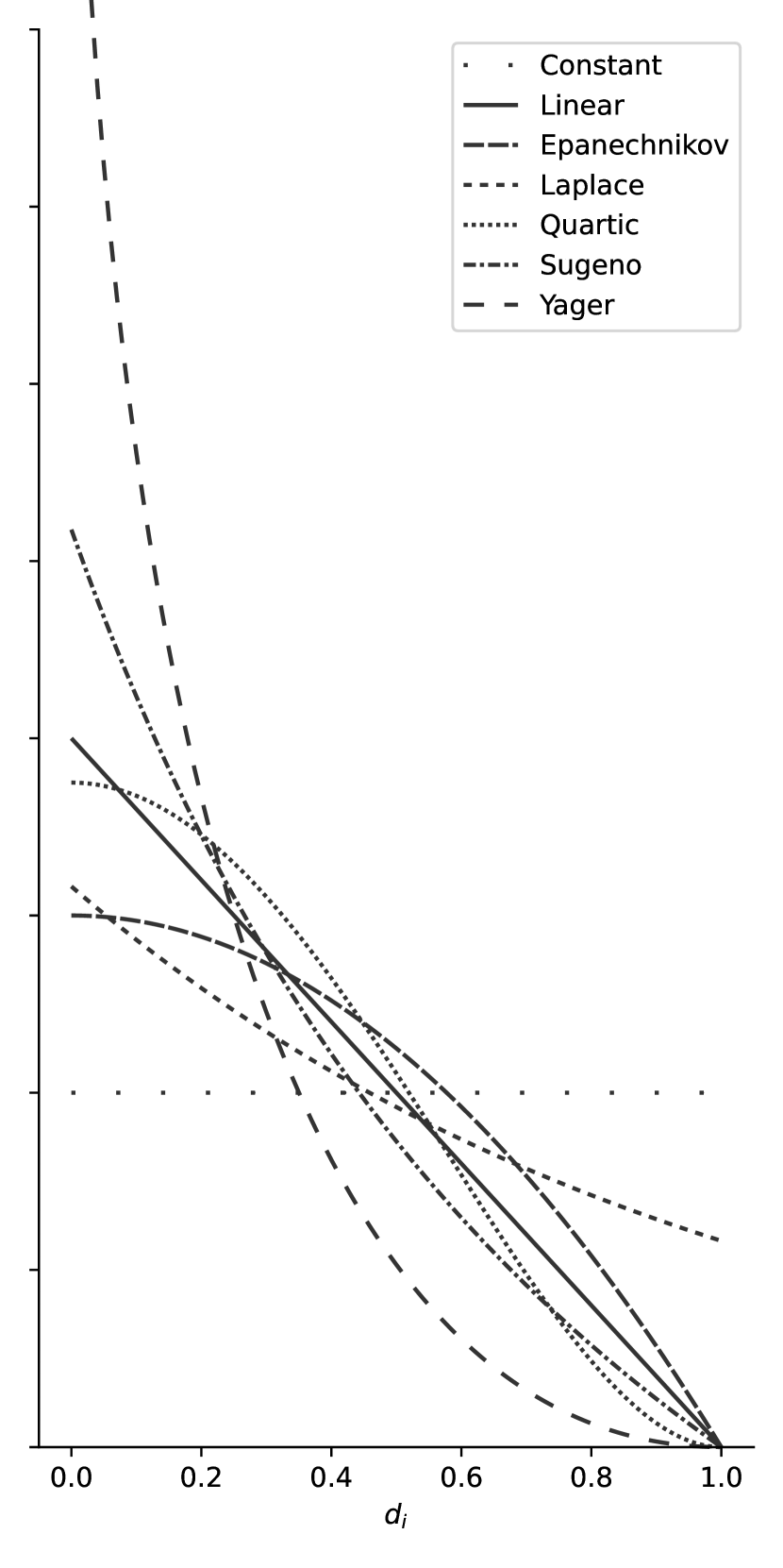
Figure 1: Proper kernels, rescaled to have common area.

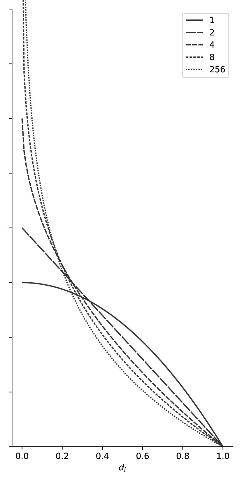
Figure 2: Samworth kernel for various dimensionalities $m$, rescaled to have common area.

We adopt the following conventions to resolve specific edge cases:

• If $d_{k}=0$ (and therefore $d_{i}=0$ for all $i\leq k$), we stipulate $d_{i}^{*}:=d_{i}=0$.

• If $d_{1}=d_{k}$ (and therefore $d_{i}^{*}=1$ for all $i\leq k$) and if $s(1)=0$, we stipulate $s(d_{i}^{*}):=1$ for all $i$.

• If $s$ is an improper kernel, and $d_{i}^{*}=0$ for some $i$, we stipulate $s(d_{i}^{*}):=1$ for all such $i$ and $s(d_{i}^{*}):=0$ for all other $i$.

When $w$ is constant, we recover NN with distance-weights, when $s$ is constant, we recover NN with rank-weights, and when both $w$ and $s$ are constant, we recover unweighted NN. In addition, in all three edge cases, we also effectively revert to performing unweighted classification with (part of) the nearest neighbours of $y$.

We will now show how this incorporates existing weighting proposals. Firstly, note that both in the original equation for NN (1), and in (2), we rescale each class score by the total sum of the weights. Therefore, we do not require that weights sum to 1. Moreover, multiplying all weights by a positive constant produces identical class scores. We will use the proportionality symbol $\propto$ to indicate that two sets of weights only differ by a positive constant factor. Thus, the linear distance-weights proposed by Dudani [9] can be simplified as follows:

$$s_{i} =\frac{d_{k}-d_{i}}{d_{k}-d_{1}}$$

$$\propto\frac{d_{k}-d_{i}}{d_{k}-d_{1}}\cdot\frac{d_{k}-d_{1}}{d_{k}}$$

$$=1-d_{i}^{*}.$$

We see that Dudani’s linear weights are equivalent to applying a linear (triangular) kernel in our revised definition. In a similar way, we can simplify the weight types proposed by Gou et al. [18]:

$$s_{i} =\frac{d_{k}-d_{i}}{d_{k}-d_{1}}\cdot\frac{d_{k}+d_{1}}{d_{k}+d_{i}}$$ (4)

$$\propto\frac{d_{k}-d_{i}}{d_{k}-d_{1}}\cdot\frac{d_{k}+d_{1}}{d_{k}+d_{i}}\cdot\frac{d_{k}-d_{1}}{d_{k}+d_{1}}\cdot\frac{1}{d_{k}}$$

$$=\frac{1-d_{i}^{*}}{1+d_{i}^{*}}.$$

For weights that depend reciprocally on nearest neighbour distance or its square, it is straightforward that

$$s_{i}=\frac{1}{d_{i}}\propto\frac{d_{k}}{d_{i}}=\frac{1}{d_{i}^{*}},$$

and

$$s_{i}=\frac{1}{d_{i}^{2}}\propto\frac{d_{k}^{2}}{d_{i}^{2}}=\frac{1}{\left(d_{i}^{*}\right)^{2}}.$$

We can also simplify the weight types proposed by MacLeod:

$$s_{i} =\frac{d_{k}-d_{i}+d_{k}-d_{1}}{2(d_{k}-d_{1})}$$

$$\propto\frac{d_{k}-d_{i}+d_{k}-d_{1}}{2(d_{k}-d_{1})}\cdot\frac{2(d_{k}-d_{1})}{d_{k}}$$

$$=2-d_{i}^{*}-d_{1}^{*}.$$

However, the resulting function still depends on $d_{1}$. That means that we can use this function to calculate distance weights, but it does not generalise to a kernel that we could also apply to rank weights.

The only distance-weights that cannot be rewritten into a kernel function are the Laplace weights $e^{-d_{i}}$ proposed in [15]. Note that these are not homogeneous, i.e. the weighting depends on the absolute scale of the distances, which is arguably undesirable. However, we can consider the kernel function $e^{-d_{i}^{*}}$.

Similarly, most types of rank weights proposed in the literature can be obtained by applying a kernel function to $\frac{i}{k+1}$. For the Samworth weights, if we fix a particular value $k>0$, and write $h=\frac{1}{k+1}$ (for reasons of space), we can define the following kernel function $f^{k}$ such that $f^{k}(\frac{i}{k+1})$ is the $i$th weight as in (2):

$$f^{k}(a)=\frac{1}{k}\left(1+\frac{m}{2}-\frac{m}{2k^{\frac{2}{m}}}\left((a/h)^{1+\frac{2}{m}}-(a/h-1)^{1+\frac{2}{m}}\right)\right).$$

$f^{k}$ is proportional to $\frac{2k}{m+2}\cdot f^{k}$, and we have the following lemma:

Lemma 1.

$$\lim_{k\rightarrow\infty}\frac{2k}{m+2}\cdot f^{k}=1-a^{\frac{2}{m}}.$$

Proof.

$$\mathrel{\phantom{=}}\lim_{k\rightarrow\infty}\frac{2k}{m+2}\cdot f_{k}$$

$$=\lim_{k\rightarrow\infty}1-\frac{m}{m+2}\cdot\frac{1}{k^{\frac{2}{m}}}\left((a/h)^{1+\frac{2}{m}}-(a/h-1)^{1+\frac{2}{m}}\right)$$

$$=1-\frac{m}{m+2}\cdot\lim_{k\rightarrow\infty}\frac{(a/h)^{1+\frac{2}{m}}-(a/h-1)^{1+\frac{2}{m}}}{k^{\frac{2}{m}}}$$

$$=1-\frac{m}{m+2}\cdot\lim_{k\rightarrow\infty}\frac{h^{1+\frac{2}{m}}}{h^{1+\frac{2}{m}}}\frac{(a/h)^{1+\frac{2}{m}}-(a/h-1)^{1+\frac{2}{m}}}{k^{\frac{2}{m}}}$$

$$=1-\frac{m}{m+2}\cdot\lim_{k\rightarrow\infty}\frac{a^{1+\frac{2}{m}}-(a-h)^{1+\frac{2}{m}}}{h\cdot\frac{k^{2/m}}{(k+1)^{2/m}}}$$

$$=1-\frac{m}{m+2}\cdot\lim_{h\rightarrow 0}\frac{a^{1+\frac{2}{m}}-(a-h)^{1+\frac{2}{m}}}{h}$$

$$=1-\frac{m}{m+2}\cdot\left(1+\frac{2}{m}\right)a^{\frac{2}{m}}$$ (*)

$$=1-a^{\frac{2}{m}},$$

where $(*)$ is the polynomial rule for derivation. ∎

Accordingly, we call $1-a^{\frac{2}{m}}$ the Samworth kernel.

The only rank weights that can not be obtained by applying a kernel function are the Fibonacci weights from [13], because their relative distribution depends on $k$.

By reformulating both distance-weights and rank-weights in terms of a kernel function, we obtain a single unique way to characterise all the different weight types. In addition, this representation makes it clear that we could also choose to apply e.g. the Sugeno kernel to obtain rank weights, or the Samworth kernel to obtain distance weights, even though they were originally proposed for, respectively, distance weights and rank weights. Furthermore, we could choose to apply both rank and distance weights at the same time, as in the proposal by Gou et al. [12], which can be realised by combining a reciprocal rank-kernel and a linear distance-kernel.

III-C Yager weights

In (4), we identified the kernel that corresponds to the weights proposed by Gou et al. [18]. This kernel is in fact Sugeno negation [30] with $\lambda=1$:

$$a\longmapsto\frac{1-a}{1+\lambda a}$$

Inspired by this, we also propose to use another type of fuzzy negation known from the literature as a weighting kernel. This negation, proposed by Higashi & Klir [29] to accompany other operators introduced by Yager [31], has the general form:

$$a\longmapsto(1-a^{p})^{\frac{1}{p}}$$

We propose to use it with $p=\frac{1}{2}$, because the resulting contour is quite different from most other kernels (Fig. 1) except the Samworth kernel for larger values of $m$ (Fig. 2).

III-D FNN

Recall that in the original proposal, there were two possible values for $u_{i}$. When $u_{i}$ is chosen crisply, the proposal simplifies to

$$\left.\sum\limits_{i\leq k|x_{i}\in C}1/d_{i}^{2/(q-1)}\middle/\sum\limits_{i\leq k}1/d_{i}^{2/(q-1)}\right..$$

In other words, it is equivalent to NN classification (1), with:

$$s_{i}=1/d_{j}^{\frac{2}{q-1}},$$

for some $q>1$. When $q=3$ and $q=2$, we obtain, respectively, reciprocal distance-weights and squared reciprocal distance-weights.

Alternatively, when $u_{i}$ is fuzzy, we have:

$$\mathrel{\phantom{=}}\left.\sum\limits_{i\leq k}u_{i}\cdot s_{i}\middle/\sum\limits_{i\leq k}s_{i}\right.$$

$$=\left.\left(\smashoperator[r]{\sum_{i\leq k|x_{i}\in C}^{}}0.51\cdot s_{i}+\sum\limits_{i\leq k}0.49\cdot n_{C}(x_{i})/k\cdot s_{i}\right)\middle/\sum_{i\leq k}s_{i}\right.$$

$$=\left.0.51\cdot\sum_{\mathclap{i\leq k|x_{i}\in C}}s_{i}\middle/\sum_{i\leq k}s_{i}\right.+\left.0.49\cdot\sum_{i\leq k}n_{C}(x_{i})/k\cdot s_{i}\middle/\sum_{i\leq k}s_{i}\right.$$

Thus, in this variant, the FNN class score is the weighted average of two components. The first component is, again, NN, while the second component is NN with fuzzified class membership. This can be rewritten as:

$$\mathrel{\phantom{=}}\left.\sum_{i\leq k}n_{C}(x_{i})/k\cdot s_{i}\middle/\sum_{i\leq k}s_{i}\right.$$

$$=\left.\frac{1}{k}\sum_{i,j\leq k|x_{ij}\in C}s_{i}\middle/\sum_{i\leq k}s_{i}\right.$$

where $x_{ij}$ is the $j$th neighbour of the $i$th neighbour of $y$. In effect, this is one more instance of NN, with class scores that are on the one hand dilluted (being based not just on the class scores of the $k$ nearest neighbours of $y$, but also on the class scores of their $k$ nearest neighbours) and on the other hand concentrated (because nearby neighbours will more frequently appear as neighbours of neighbours).

III-E FRNN

The upper and lower approximations of FRNN can similarly be rewritten using kernel functions:

Definition 3.

Let $d$ be a distance measure and $k$ a positive integer, $w$ a choice of kernel function and $s$ a choice of fuzzy negation. Then the score for a decision class $C$ and a test record $y$ is:

$$\begin{aligned} \overline{C}(y)&:=\left.\sum_{i\leq k}w_{i}^{k}\cdot s(\min(d_{i}^{+}/d_{*}^{+},1))\middle/\sum_{i\leq k}w_{i}^{k}\right.;\\ \underline{C}(y)&:=\left.\sum_{i\leq k}w_{i}^{k}\cdot(1-s(\min(d_{i}^{-}/d_{*}^{-},1)))\middle/\sum_{i\leq k}w_{i}^{k}\right.,\end{aligned}$$

where $d^{+}_{i}$ and $d^{-}_{i}$ are the $i$th nearest neighbour distance of $y$ in, respectively, $C$ and $X\setminus C$, and $d^{+}_{*}$ and $d^{-}_{*}$ are to be defined.

$d_{*}^{+}$ and $d_{*}^{-}$ determine cutoff values — all larger distances are mapped to the minimum degree of similarity, typically 0. These values have to be constant across decision classes and test records, to allow for a proper comparison of class scores. If we choose values that are too small, $\min(d_{i}^{+}/d_{*}^{+},1)$ and $\min(d_{i}^{-}/d_{*}^{-},1)$ become equal to 1 for many test records and many values of $i$, and we lose information. If we choose values that are too large, $\min(d_{i}^{+}/d_{*}^{+},1)$ and $\min(d_{i}^{-}/d_{*}^{-},1)$ are generally close to $0$, and we do not make full use of the profile of the kernel $s$. Therefore, as a compromise, we calculate $d_{k}^{+}$ and $d_{k}^{-}$ of all training records, for all decision classes, and take $d_{*}^{+}$ and $d_{*}^{-}$ to be the respective maxima of these values.

Note that unlike NN, FRNN cannot be used with constant distance-weights, because this would equalise all class scores. Instead, the default choice is linear distance-weights, in which case the double negation $(1-s(d_{i}))$ in the lower approximation simplifies to $d_{i}$. In addition, the exponentially decreasing rank-weights that have occasionally been proposed in the literature have a very limited usefulness, as the contribution of each additional value quickly becomes insignificant, and, eventually, impossible to compute.

III-F Distance and scaling measures

Three distance measures that are frequently used with nearest neighbour classification are Euclidean, Boscovich (or city-block) and Chebyshev (or maximum) distance. These can be viewed, respectively, as the special cases $p=2$, $p=1$ and $p\rightarrow\infty$ of the Minkowski $p$-distance between two points $x,y\in\mathbb{R}^{m}$ (for some $m\geq 1$):

$$\left|y-x\right|_{p}:=\left(\sum_{i\leq m}\left|y_{i}-x_{i}\right|^{p}\right)^{\frac{1}{p}}.$$

In order to obtain a comparable contribution from all attributes, these must be rescaled to a common scale. This can be done by taking a measure of dispersion, and dividing each attribute by this measure, such that it becomes 1 for each attribute. Two common choices are the standard deviation and the range of each attribute. These can be linked to the concept of Minkowski $p$-distance by defining the Minkowski $p$-centre and $p$-radius of a dataset:

Definition 4.

Let $X=(x_{1},x_{2},\dots,x_{n})$ be a univariate real-valued dataset. The Minkowski $p$-radius $r_{p}$ of $X$ is defined as:

$$r_{p}(X):=\min_{z\in\mathbb{R}}\left(\frac{1}{n}\sum_{i\leq n}\left|x_{i}-z\right|^{p}\right)^{\frac{1}{p}},$$

while the Minkowski $p$-centre of $X$ is the corresponding minimising value for $z$ (not necessarily unique for $p\leq 1$).

The standard deviation and half-range of a dataset are $r_{2}$ and $r_{\infty}$, while the corresponding $2$-centre and $\infty$-centre of a dataset are its mean and its midrange. The $1$-centre of a dataset is its median, and the corresponding measure of dispersion $r_{1}$ that it minimises is the mean absolute deviation around the median. Thus, $r_{1}$ is another measure of dispersion that we can use to scale attributes with.

A potential advantage of $r_{1}$-scaling over $r_{2}$-scaling is its reduced sensitivity to outliers, as $r_{1}$ only depends linearly on outliers, rather than quadratically like $r_{2}$. In turn, both measures are much less sensitive to outliers than $r_{\infty}$, which is completely determined by the most extreme outlier. An alternative way to obtain a measure of dispersion that is less sensitive to outliers that is sometimes used in the literature is to explicitly ignore peripheral values, by only considering half the interquartile range, which we will designate by $r_{\infty}^{*}$.

IV Experimental setup

TABLE II: Real-life Classification Datasets from the UCI Repository for Machine Learning.

Dataset	Records	Classes	Attributes	Imbalance ratio	Dataset	Records	Classes	Attributes	Imbalance ratio
accent	329	6	12	2.5	mfeat	2000	10	649	1.0
acoustic-features	400	4	50	1.0	miniboone	130 064	2	50	2.6
ai4i2020	10 000	2	6	28.5	new-thyroid	215	3	5	3.5
alcohol	125	5	12	1.0	oral-toxicity	8992	2	1024	11.1
androgen-receptor	1687	2	1024	7.5	page-blocks	5473	5	10	31.6
avila	20 867	12	10	38.7	phishing-websites	11 055	2	30	1.3
banknote	1372	2	4	1.2	plrx	182	2	12	2.5
bioaccumulation	779	3	9	4.3	pop-failures	540	2	18	10.7
biodeg	1055	2	41	2.0	post-operative	87	2	8	2.6
breasttissue	106	6	9	1.3	qualitative-bankruptcy	250	2	6	1.3
ca-cervix	72	2	19	2.4	raisin	900	2	7	1.0
caesarian	80	2	5	1.4	rejafada	1996	2	6824	1.0
ceramic	37	4	34	1.4	rice	3810	2	7	1.3
cmc	1473	3	9	1.6	seeds	210	3	7	1.0
codon-usage	13 011	20	64	25.5	segment	2310	7	19	1.0
coimbra	116	2	9	1.2	seismic-bumps	2584	2	18	14.2
column	310	3	6	1.9	sensorless	58 509	11	48	1.0
debrecen	1151	2	19	1.1	sepsis-survival	110 204	2	3	12.6
dermatology	358	6	34	2.2	shuttle	58 000	7	9	560.8
diabetes-risk	520	2	16	1.6	skin	245 057	2	3	3.8
divorce	170	2	54	1.0	somerville	143	2	6	1.2
dry-bean	13 611	7	16	2.3	sonar	208	2	60	1.1
ecoli	332	6	7	6.3	south-german-credit	1000	2	20	2.3
electrical-grid	10 000	2	12	1.8	spambase	4601	2	57	1.5
faults	1941	7	27	3.9	spectf	267	2	44	3.9
fertility	100	2	9	7.3	sportsarticles	1000	2	59	1.7
flowmeters	361	4	44	1.7	sta-dyn-lab	6248	2	244	9.5
forest-types	523	4	9	1.8	tcga-pancan-hiseq	801	5	20 531	1.9
gender-gap	3145	2	15	7.9	thoraric-surgery	470	2	16	5.7
glass	214	6	9	3.6	transfusion	748	2	4	3.2
haberman	306	2	3	2.8	tuandromd	4464	2	241	4.0
hcv	589	2	12	9.5	urban-land-cover	675	9	147	2.2
heart-failure	299	2	12	2.1	vehicle	846	4	18	1.1
house-votes-84	435	2	16	1.6	warts	180	2	8	2.0
htru2	17 898	2	8	9.9	waveform	5000	3	21	1.0
ilpd	579	2	10	2.5	wdbc	569	2	30	1.7
ionosphere	351	2	34	1.8	wifi	2000	4	7	1.0
iris	150	3	4	1.0	wilt	4839	2	5	17.5
landsat	6435	6	36	1.7	wine	178	3	13	1.3
leaf	340	30	14	1.2	wisconsin	683	2	9	1.9
letter	20 000	26	16	1.0	wpbc	138	2	32	3.9
lrs	527	7	100	12.6	yeast	1484	10	8	11.6
magic	19 020	2	10	1.8

To evaluate NN, FNN and FRNN classification, we will use 85 numerical real-life datasets from the UCI repository for machine learning (Table II). We perform 5-fold cross-validation, and calculate the mean AUROC as a measure of the discriminative ability of each classifier. To compare two alternatives, we calculate the $p$-value from a one-sided Wilcoxon signed-rank test. Where appropriate, we also apply the Holm-Bonferroni method [32] to correct for family-wise error.

For all of NN, FNN and FRNN, we optimise $k$ through leave-one-out validation, which can be performed efficiently for nearest neighbour classifiers by executing a $k+1$-nearest neighbour query on the training set and eliminating all matches between a training record and itself. For FRNN, we also choose between the upper, lower or mean approximation based on validation AUROC.

V Results

In this section, we will present the results of our experiments. To start with, we will evaluate distance measures, scaling measures and weight types, but restrict ourselves to the weight types that have previously been proposed in the literature. We will then ask whether these results can be further improved upon by using the Yager weights that we have proposed.

V-A NN

We first consider the effect of the distance on classification performance. We find that for all types of scaling and all weight types, Boscovich distance leads to significantly better performance than Euclidean ($p<0.0031$) and Chebyshev ($p<1.6\cdot 10^{-9}$) distance. For this reason, we will only consider Boscovich distance for the rest of our analysis.

Next, we have a look at the different kernels. First we compare using each kernel for distance-weights versus rank-weights, for each type of scaling. With two exceptions, we find that distance-weights lead to significantly better classification performance than rank-weights ($p<0.0019$). The exceptions are the reciprocal and Laplace kernels, for which the difference is not or only weakly significant, and to which we return below.

TABLE III: One-sided $p$-values, Samworth distance-weights vs other distance-weights, for NN with Boscovich distance, in terms of AUROC. Holm-Bonferroni family-wise error correction applied to each column.

Samworth vs…	Scaling
	$r_{1}$	$r_{2}$	$r_{\infty}$	$r_{\infty}^{*}$
Constant	$<0.0001$	$<0.0001$	$<0.0001$	$<0.0001$
Epanechnikov	$0.00051$	$0.00016$	$<0.0001$	$<0.0001$
Laplace	$<0.0001$	$<0.0001$	$<0.0001$	$<0.0001$
Linear	$0.00016$	$0.00030$	$0.00048$	$<0.0001$
MacLeod	$<0.0001$	$<0.0001$	$<0.0001$	$<0.0001$
Quartic	$0.014$	$0.11$	$0.71$	$0.042$
Reciprocally linear	$0.0012$	$0.00016$	$<0.0001$	$<0.0001$
Reciprocally quadratic	$0.038$	$0.020$	$0.046$	$0.059$
Sugeno	$0.0068$	$0.0036$	$0.029$	$0.00036$

Among the distance-weights, the Samworth kernel significantly outperforms all other kernels (Table III), with three exceptions. The difference with respect to the quartic and reciprocally squared kernel is only weakly significant with, respectively, $r_{2}$ and $r_{\infty}^{*}$ scaling. Moreover, with $r_{\infty}$ scaling, the quartic kernel is actually slightly better than the Samworth kernel on our data, but we will see below that $r_{\infty}$ scaling is suboptimal. Finally, we also find that Samworth distance weights outperform reciprocal ($p<0.0048$) and Laplace ($p<6.2\cdot 10^{-6}$) rank weights across scaling measures.

Samworth distance-weights also significantly outperform the combination of linear distance-weights and reciprocal rank-weights proposed by Gou et al. [12] for all scaling types ($p<0.044$) except $r_{\infty}$, where the difference is only weakly significant ($p=0.13$). However, our general formula for NN classification also allows for other combinations. Indeed, we find that Samworth distance-weights are outperformed by the logical combination of Samworth distance-weights and Samworth rank-weights ($p<0.040$).

TABLE IV: One-sided $p$-values, various scalings vs $r_{\infty}$-scaling, for NN with Boscovich distance and Samworth distance- and rank-weights, in terms of AUROC. Holm-Bonferroni family-wise error correction applied.

Test	p
$r_{2}$ vs $r_{\infty}$	$0.00043$
$r_{1}$ vs $r_{\infty}$	$0.023$
$r_{\infty}^{*}$ vs $r_{\infty}$	$0.023$

Finally, when we consider the different measures of dispersion that can be used to normalise a dataset through rescaling, we find that $r_{1}$, $r_{2}$ and $r_{\infty}^{*}$ do not significantly outperform each other for the combination of Samworth distance- and rank-weights, while they all outperform $r_{\infty}$ (Table IV). For other weight types, we obtain comparable results.

V-B FNN

For FNN, we will consider reciprocally linear and reciprocally squared distance-weights, as well as Samworth distance-weights and a combination of Samworth rank- and distance-weights, since we found in the previous Subsection that these latter two perform well for classical NN.

As with NN, FNN performs significantly better with Boscovich distance than with either Euclidean ($p<0.025$) or Chebyshev ($p<8.3\cdot 10^{-7}$) distance.

TABLE V: One-sided $p$-values, Samworth distance-weights vs other distance-weights, for FNN with Boscovich distance, in terms of AUROC. Holm-Bonferroni family-wise error correction applied to each column.

Samworth vs…	Scaling
	$r_{1}$	$r_{2}$	$r_{\infty}$	$r_{\infty}^{*}$
Reciprocally linear	$0.028$	$0.17$	$0.012$	$0.68$
Reciprocally quadratic	$0.34$	$0.32$	$0.18$	$0.69$

Unlike NN, it is not clear that Samworth distance-weights perform better than reciprocally linear or reciprocally squared weights (Table V). Furthermore, the combination of Samworth rank- and distance-weights actually performs worse than Samworth distance-weights alone for $r_{1}$ ($p=0.032$) and $r_{\infty}$ ($p=0.000078$) scaling, while for $r_{2}$ and $r_{\infty}^{*}$ scaling, the difference is not significant.

TABLE VI: One-sided $p$-values, comparing the scaler in each row against the scaler in each column, for FNN with Boscovich distance and Samworth distance-weights, in terms of AUROC. Holm-Bonferroni family-wise error correction applied to each row.

	$r_{2}$	$r_{\infty}$	$r_{\infty}^{*}$
$r_{1}$	$0.19$	$0.14$	$0.14$
$r_{2}$		$0.21$	$0.21$
$r_{\infty}$			$0.97$

We have weak evidence that with FNN, $r_{1}$ scaling leads to better performance than $r_{2}$ scaling, and that in turn both are preferable over $r_{\infty}$ and $r_{infty}^{*}$ scaling (Table VI).

V-C FRNN

For FRNN, we will evaluate the different types of rank-weights proposed in the literature, corresponding to the constant, linear and reciprocal kernel, in combination with linear distance-weights. In addition, we evaluate Samworth rank- and distance-weights, motivated by their excellent performance with NN.

Here we also find that Boscovich distance leads to higher AUROC than Euclidean ($p<0.00086$) and Chebyshev ($p<6.2\cdot 10^{-10}$) distance for all combinations of kernels and scaling measures.

TABLE VII: One-sided $p$-values, Samworth vs linear distance-weights, for FRNN with Boscovich distance and various rank-weights and scalings.

Rank kernel	Scaling
	$r_{1}$	$r_{2}$	$r_{\infty}$	$r_{\infty}^{*}$
Constant	$<0.0001$	$<0.0001$	$<0.0001$	$<0.0001$
Linear	$<0.0001$	$<0.0001$	$<0.0001$	$<0.0001$
Reciprocally linear	$0.082$	$0.12$	$0.061$	$0.0061$
Samworth	$0.0012$	$0.00018$	$0.00043$	$<0.0001$

TABLE VIII: One-sided $p$-values, Samworth rank-weights vs other rank-weights, for FRNN with Boscovich distance and Samworth distance-weights. Holm-Bonferioni correction applied in each column.

Samworth vs…	Scaling
	$r_{1}$	$r_{2}$	$r_{\infty}$	$r_{\infty}^{*}$
Constant	$0.18$	$0.0033$	$0.089$	$0.0048$
Linear	$0.18$	$0.070$	$0.72$	$0.32$
Reciprocally linear	$0.18$	$0.022$	$0.15$	$0.057$

The traditional choice for distance-weights is to use a linear kernel, but we find that the Samworth kernel performs better, although the difference is only weakly significant in combination with reciprocal rank-weights (Table VII).

Likewise, Samworth rank-weights appear to be the best choice, but the advantage over other kernels is only weakly significant (Table VIII).

TABLE IX: One-sided $p$-values, various scalings vs $r_{\infty}$-scaling, for FRNN with Boscovich distance and Samworth distance- and rank-weights, in terms of AUROC. Holm-Bonferroni family-wise error correction applied.

Test	p
$r_{2}$ vs $r_{\infty}$	$0.0078$
$r_{1}$ vs $r_{\infty}$	$0.060$
$r_{\infty}^{*}$ vs $r_{\infty}$	$0.060$

As with NN, the measures of dispersion $r_{1}$, $r_{2}$ and $r_{\infty}^{*}$ do not significantly outperform each other, but do outperform $r_{\infty}$, although even this latter fact is only weakly significant (Table IX).

V-D NN vs FNN vs FRNN

TABLE X: One-sided $p$-values, NN vs FNN with Boscovich distance and various distance kernels and scalings, in terms of AUROC.

Distance kernel	Scaling
	$r_{1}$	$r_{2}$	$r_{\infty}$	$r_{\infty}^{*}$
Reciprocally linear	$<0.0001$	$<0.0001$	$<0.0001$	$<0.0001$
Reciprocally quadratic	$<0.0001$	$<0.0001$	$<0.0001$	$<0.0001$
Samworth	$<0.0001$	$<0.0001$	$<0.0001$	$<0.0001$

In Subsection V-B, we observed that FNN performs best on our data with Samworth distance-weights, but that the difference with respect to reciprocally linear and reciprocally square distance-weights is not significant for all scaling-types. However, when we compare FNN to NN, we find that for all three kernels, NN performs significantly better (Table X).

TABLE XI: One-sided $p$-values, FRNN vs NN, Boscovich distance and Samworth rank- and distance-weights.

Scaling
$r_{1}$	$r_{2}$	$r_{\infty}$	$r_{\infty}^{*}$
$0.021$	$0.0092$	$0.0051$	$0.049$

For both NN and FRNN, we obtained the best results with a combination of Samworth distance- and rank-weights. When we compare NN and FRNN against each other, we find that FRNN performs better (Table XI).

V-E Yager weights

We now consider the results of the Yager kernel that we have proposed.

When we equip NN with both Yager distance- and rank-weights, this performs slightly better on our data than Samworth distance- and rank-weights, but the difference is not significant ($p<0.25$ accross scaling measures). Interestingly, unlike the Samworth kernel, the Yager kernel appears to perform about as well when only used for distance-weights and when used for both distance- and rank-weights. Correspondingly, Yager distance-weights perform significantly better than Samworth distance-weights ($p<0.0053$). Thus the main advantage of the Yager kernel is that it enables comparable performance as the Samworth kernel, but is easier to implement, because it does not require the addition of rank-weights and because it is not dependent on the dimensionality of the dataset.

In contrast, for FNN we obtain comparable performance between Samworth and Yager distance-weights with $r_{1}$ or $r_{2}$ scaling, and for FRNN we find that Samworth distance- and rank-weights still perform significantly better than Yager distance- and rank-weights ($p<0.050$ across scaling measures).

VI Conclusion

In this paper, we have provided a comprehensive overview of the different weighting variants of NN, FNN and FRNN classification that have been proposed in the literature. We have proposed a uniform framework for these proposals and conducted an evaluation on 85 real-life datasets. This allows us to draw the following conclusions

• Weighting can be expressed as the application of a kernel function to the distances and/or ranks of the nearest neighbours of a test record — we have provided an overview of kernel functions that correspond to existing weighting proposals in the literature.

• In particular, Samworth rank-weights, which have been shown to be theoretically optimal, converge to a kernel function that depends on the dimensionality of the data, and that can also be applied to obtain distance-weights.

• On real-life datasets, both NN and FRNN perform better with a combination of Samworth rank- and distance-weights than with other weight types proposed in the literature, while FNN appears to perform best with Samworth distance-weights and constant rank-weights.

• However, NN and FNN appear to perform equally well with Yager weights, a novel weight type inspired by fuzzy Yager negation. For NN, the Yager kernel offers two practical benefits over the Samworth kernel: it only needs to be applied to obtain distance weights (not rank weights), and it does not depend on the dimensionality of the dataset. For FRNN, Samworth weights still perform better.

• Boscovich distance clearly outperforms Euclidean and Chebyshev distance, regardless of other hyperparameter choices.

• With Samworth and Yager weights, rescaling attributes by $r_{1}$ (mean absolute deviation around the median), $r_{2}$ (standard deviation) or $r_{\infty}^{*}$ (interquartile half-range) produces comparable results, while these are all better than rescaling by $r_{\infty}$ (half-range).

• Our comparison between NN and FNN with identical distance-weights reveals that in practice, the fuzzification of class membership degrees in FNN leads to systematically lower performance. In contrast, with its more fundamentally different approach, FRNN does generally outperform NN when both are equipped with their best-performing weighting scheme (Samworth distance- and rank-weights).

We believe that these results serve as a useful baseline for future applications and research. For applications, we recommend the use of FRNN classification with Samworth rank- and distance weights, Boscovich distance, and any one of $r_{1}$-, $r_{2}$- or $r_{\infty}^{*}$-scaling, while $k$ can be optimised through efficient leave-one-out validation. With the classical NN algorithm, we recommend the same hyperparameter choices, except that Yager distance-weights may be substituted and rank-weights omitted.

We suggest that future research should concentrate on identifying even better-performing kernel functions. For this, the contours of the Samworth and Yager kernels may serve as a useful starting point. In particular, we hope that in this way the following two questions may be answered:

• Should an optimal kernel depend on the dimensionality of the data? The good performance of the Samworth kernel suggests that the answer is yes. However, we note that its profile is actually very similar for typical dimensionalities of $4\leq m\leq 256$, so that its variation according to dimensionality may be far less important than the basic outline of its profile. This is seemingly confirmed by the relatively strong performance of the Yager kernel, which has a similar profile.

• For NN, do we need both distance- and rank- weights? The fact that Yager distance-weights alone perform as well as a combination of Samworth distance- and rank-weights suggests that with the right kernel, we can do away with rank-weights.

We hope that any future evaluations of competing proposals will be based on a similar collection of real-life classification problems to the one that we have assembled, which we have made available for this purpose.

Data

The datasets used in this paper can be downloaded from https://cwi.ugent.be/~oulenz/datasets/lenz-2024-unified.tar.gz.

References

- [1] E. Fix and J. Hodges, Jr, “Discriminatory analysis — nonparametric discrimination: Consistency properties,” USAF School of Aviation Medicine, Randolph Field, Texas, Technical report 21-49-004, 1951.
- [2] J. M. Keller, M. R. Gray, and J. A. Givens, “A fuzzy -nearest neighbor algorithm,” IEEE Trans. Syst., Man, Cybern., no. 4, pp. 580–585, 1985.
- [3] R. Jensen and C. Cornelis, “A new approach to fuzzy-rough nearest neighbour classification,” in Proc. 6th Int. Conf. Rough Sets Current Trends Comput., 2008, pp. 310–319.
- [4] R. J. Samworth, “Optimal weighted nearest neighbour classifiers,” Ann. Statist., pp. 2733–2763, 2012.
- [5] G. S. Watson, “Smooth regression analysis,” Sankhyā: Indian J. Statist., Ser. A, pp. 359–372, 1964.
- [6] R. M. Royall, “A class of non-parametric estimates of a smooth regression function.” Ph.D. dissertation, 1966.
- [7] D. Shepard, “A two-dimensional interpolation function for irregularly-spaced data,” in Proc. 1968 23rd ACM Nat. Conf., 1968, pp. 517–524.
- [8] M. Rosenblatt, “Remarks on some nonparametric estimates of a density function,” Ann. Math. Statist., pp. 832–837, 1956.
- [9] S. A. Dudani, “An experimental study of moment methods for automatic identification of three-dimensional objects from television images,” Ph.D. dissertation, The Ohio State University, 1973.
- [10] ——, “The distance-weighted -nearest-neighbor rule,” IEEE Trans. Syst., Man, Cybern., vol. 6, no. 4, pp. 325–327, 1976.
- [11] C. J. Stone, “Consistent nonparametric regression,” Ann. Statist., pp. 595–620, 1977.
- [12] J. Gou, T. Xiong, and Y. Kuang, “A novel weighted voting for k-nearest neighbor rule.” J. Comput., vol. 6, no. 5, pp. 833–840, 2011.
- [13] T.-L. Pao, Y.-T. Chen, J.-H. Yeh, Y.-M. Cheng, and Y.-Y. Lin, “A comparative study of different weighting schemes on KNN-based emotion recognition in Mandarin speech,” in 3rd Int. Conf. Intell. Comput., 2007, pp. 997–1005.
- [14] R. N. Shepard, “Toward a universal law of generalization for psychological science,” Science, vol. 237, no. 4820, pp. 1317–1323, 1987.
- [15] J. Zavrel, “An empirical re-examination of weighted voting for -NN,” in Proc. 7th Belg.-Dutch Conf. Mach. Learn., 1997, pp. 139–145.
- [16] T. Bailey and A. Jain, “A note on distance-weighted -nearest neighbor rules,” IEEE Trans. Syst., Man, Cybern., vol. 8, no. 4, pp. 311–313, 1978.
- [17] J. E. Macleod, A. Luk, and D. M. Titterington, “A re-examination of the distance-weighted k-nearest neighbor classification rule,” IEEE Trans. Syst., Man, Cybern., vol. 17, no. 4, pp. 689–696, 1987.
- [18] J. Gou, L. Du, Y. Zhang, T. Xiong et al., “A new distance-weighted k-nearest neighbor classifier,” J. Inf. Comput. Sci., vol. 9, no. 6, pp. 1429–1436, 2012.
- [19] K. Hechenbichler and K. Schliep, “Weighted -nearest-neighbor techniques and ordinal classification,” Ludwig-Maximilians-Universität München, Institut für Statistik, Sonderforschungsbereich 386, Paper 399, 2004.
- [20] J. Derrac, S. García, and F. Herrera, “Fuzzy nearest neighbor algorithms: Taxonomy, experimental analysis and prospects,” Inf. Sci., vol. 260, pp. 98–119, 2014.
- [21] D. Dubois and H. Prade, “Rough fuzzy sets and fuzzy rough sets,” Int. J. General Syst., vol. 17, no. 2-3, pp. 191–209, 1990.
- [22] Z. Pawlak, “Rough sets,” ICS PAS, Report 431, 1981.
- [23] C. Cornelis, N. Verbiest, and R. Jensen, “Ordered weighted average based fuzzy rough sets,” in Proc. 5th Int. Conf. Rough Set Knowl. Technol., 2010, pp. 78–85.
- [24] O. U. Lenz, D. Peralta, and C. Cornelis, “Scalable approximate FRNN-OWA classification,” IEEE Trans. Fuzzy Syst., vol. 28, no. 5, pp. 929–938, 2020.
- [25] N. Verbiest, C. Cornelis, and F. Herrera, “Selección de prototipos basada en conjuntos rugosos difusos,” in 16. Congreso Español sobre Tecnologías y Lógica Fuzzy, 2012, pp. 638–643.
- [26] N. Verbiest, “Fuzzy rough and evolutionary approaches to instance selection,” Ph.D. dissertation, Universiteit Gent, 2014.
- [27] S. Vluymans, N. Mac Parthaláin, C. Cornelis, and Y. Saeys, “Weight selection strategies for ordered weighted average based fuzzy rough sets,” Inf. Sci., vol. 501, pp. 155–171, 2019.
- [28] D. Wettschereck, “A study of distance-based machine learning algorithms,” Ph.D. dissertation, Oregon State University, 1994.
- [29] M. Higashi and G. J. Klir, “On measures of fuzziness and fuzzy complements,” Int. J. General Syst., vol. 8, no. 3, pp. 169–180, 1982.
- [30] M. Sugeno, “Constructing fuzzy measure and grading similarity of patterns by fuzzy integral,” Trans. Soc. Instrum. Control Engineers, vol. 9, no. 3, pp. 361–368, 1973.
- [31] R. R. Yager, “On a general class of fuzzy connectives,” Fuzzy Sets Syst., vol. 4, no. 3, pp. 235–242, 1980.
- [32] S. Holm, “A simple sequentially rejective multiple test procedure,” Scand. J. Statist., vol. 6, no. 2, pp. 65–70, 1979.