Data-efficient operator learning for solving high Mach number fluid flow problems

Abstract

We consider the problem of using scientific machine learning (SciML) to predict solutions of high Mach fluid flows over irregular geometries. In this setting, data is limited, and so it is desirable for models to perform well in the low-data setting. We show that the neural basis function (NBF), which learns a basis of behavior modes from the data and then uses this basis to make predictions, is more effective than a basis-unaware baseline model. In addition, we identify continuing challenges in the space of predicting solutions for this type of problem.

1 Introduction

Scientific models enable scientists and engineers to study complex systems of interest, such as animal brains (1), bacteria growth (2), and fluid dynamics (3). These models are typically computationally intensive, which limits how much they can be used. An increasingly-common alternative is to supplement these models with scientific machine learning (SciML) approaches (4) that incorporate an inductive bias to improve data efficiency. Examples of physics-informed inductive biases include the physics-informed deep operator network (DeepONet) (5; 6) and physics-informed neural operator (PINO) (7), or the POD-ONet (principal orthogonal decomposition deep operator network) (8). Another type of inductive bias is the use of basis functions to form the model predictions, which limits the model’s expressiveness. In this paper, we explore use of basis functions and this bias’ effect on predictive performance.

In this work, we analyze high-Mach fluid flow over a blunt nose cone (Figure 1(a), with further details in Appendix A). Compared to other SciML settings: (1) There are no existing large-scale databases for its behavior, (2) it has a non-uniform geometry, and (3) its high-Mach fluid flows create complex physical features like boundary layers. Thus, we rely on an implementation of the recent neural basis function (NBF) (9) as our primary SciML model, which has been applied to similar problems before, while also comparing to a DeepONet (10)-like architecture that lacks scientific regularization. In this study, we do not use scientific regularization when fitting the NBF. By omitting scientific regularization, we increase the NBF’s similarity to the physics-unaware DeepONet, improving the comparability of the two models.

The NBF combines the DeepONet with ideas from reduced order modeling (ROM), in particular the principal orthogonal decomposition (POD) (11), to first learn a basis representation for the system’s state variables and then an additional set of functions that combine the basis representation into variable predictions. The basis acts as a form of regularization that helps deal with complex physical features. Similar techniques have been used, e.g., the POD-DeepONet (8).

Compared to a basis-unaware DeepONet, the basis regularization of the NBF improves the relative prediction error in the low-data regime when predicting solutions to high Mach fluid flow problems (Table 1). However, both models are unable to fully fit the training data (Table 2). Additionally, accurate prediction of the density variable $\rho$ is difficult, due to its highly skewed distribution. This motivates the need for further development in expressive neural architectures and training schemes that can learn complex distributions of partial differential equation (PDE) behavior.

2 Methods

2.1 Problem setup

We consider a dataset $\mathcal{D}$ that consists of sets $(X,W^{d},\psi^{d}),d=1,\ldots,D$, where $X=\{x_{n}\}_{n=1}^{N}\subseteq\Omega\subseteq\mathbb{R}^{N_{x}}$ is a spatial mesh over an irregular geometry $\Omega$, shared across all sets, $W^{d}=\{w^{d}_{n}\}_{n=1}^{N}\subseteq\mathbb{R}^{N_{w}}$ is a set of state variables values (with $w^{d}_{n}$ the value at mesh point $x^{d}_{n}$), and $\psi^{d}\in\mathbb{R}^{N_{\psi}}$ is a parameter vector. We learn models $\hat{w}_{\ell}$, one for each state variable $\ell=1,\ldots,N_{w}$.

In our setting (Appendix A), data satisfy compressible Navier-Stokes equations (NSE) (Appendix C) defined over a 3D axisymmetric geometry (Figure 1), based on the Radio Attenuation Measurement (RAM)-C II flight vehicle (12; 13). Due to the axisymmetry, there are two spatial inputs ($N_{x}=2$). We model four state variables: $x$-velocity ($u_{1}$), $y$-velocity ($u_{2}$), density ($\rho$), and temperature ($T$). The parameter vector $\psi$ has two components: Mach and altitude. Each solution is resolved on a mesh of $N=160250$ spatial points.

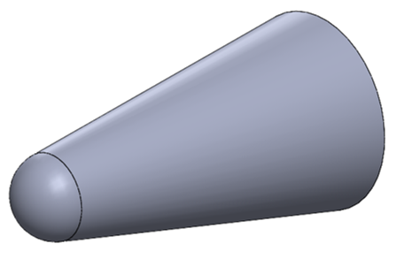
(a) The RAM-C II blunt nose cone

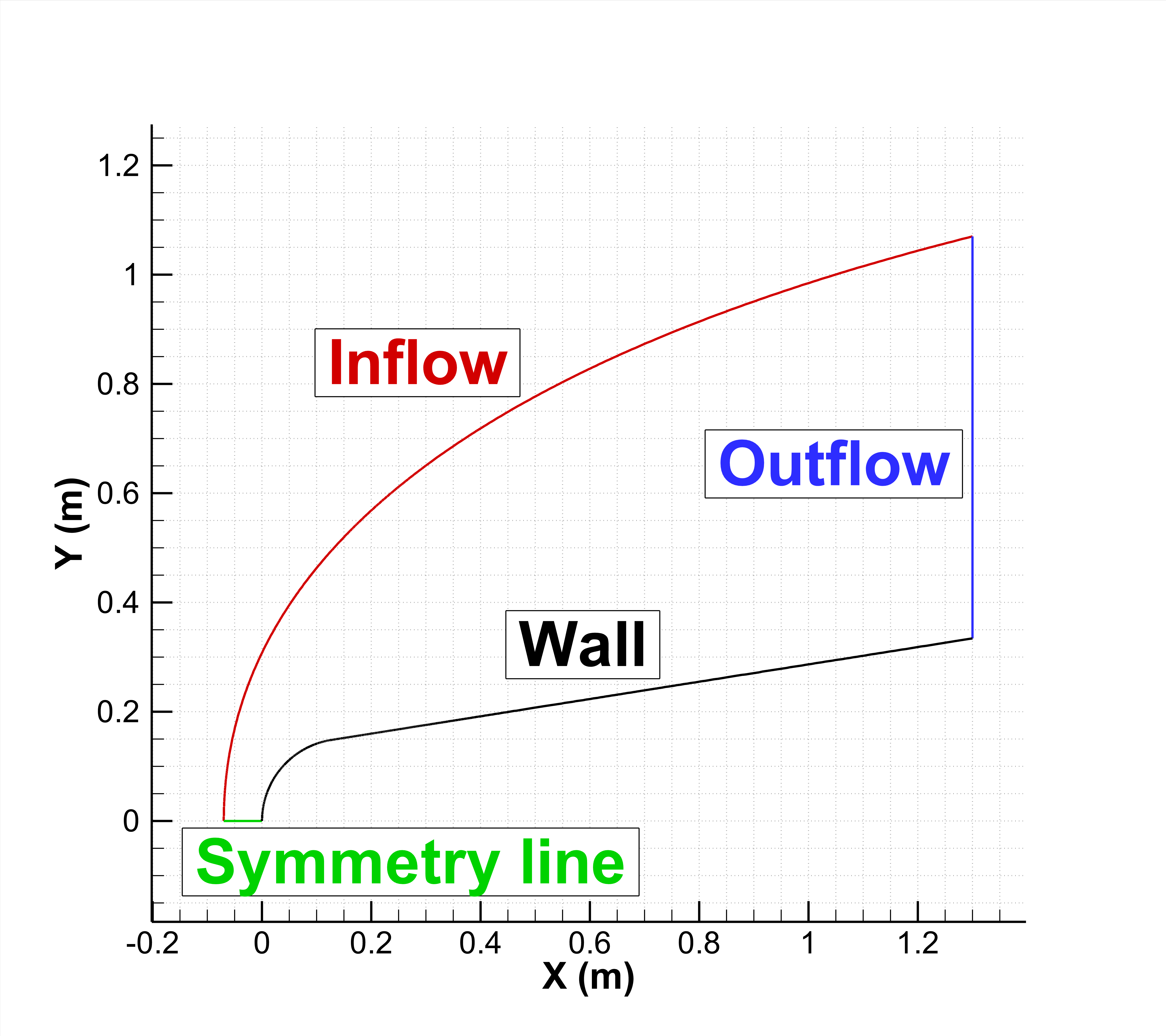
(b) The domain components

Figure 1: The RAM-C II geometry

2.2 ML models for predicting high Mach fluid flow

To solve the RAM-C II fluid flow problem, we rely on two types of SciML model. The first is a physics-unaware DeepONet (10), and the second is an implementation of the NBF (9).

For a state variable $\ell$, the DeepONet $\hat{w}_{\ell}^{\text{ONet}}$ is a composition of multi-layer perceptrons (MLPs):

$$(x,\psi)\mapsto f_{d}(f_{x}(x)\odot f_{\psi}(\psi)),$$ (1)

where $\odot$ is element-wise multiplication, $f_{x}$ is an encoder for the spatial points $x$, $f_{\psi}$ is an encoder for the PDE parameters $\psi$, and $f_{d}$ is a decoder for the predicted state variable. MLPs have $\tanh$ activation functions. Each $\hat{w}_{\ell}^{\text{ONet}}$ is trained by using stochastic gradient descent (SGD) and the Adam (14) optimizer over tuples $(x_{n},\psi^{d},w^{d}_{n})$ to minimize the squared errors $|w^{d}_{n,\ell}-\hat{w}_{\ell}^{\text{ONet}}(x_{n},\psi^{d})|^{2}$.

Like the DeepONet, for the NBF, a state variable’s predictive model $\hat{w}_{\ell}^{\text{NBF}}$ is based on a set of MLPs:

$$(x,\psi)\mapsto\sum_{j=1}^{N_{bf}}C_{j,\ell}(\psi)\phi_{j,\ell}(x),$$ (2)

where $\phi_{j,\ell}$ and $C_{j,\ell}$ are MLPs. The $\phi_{j,\ell}$ are basis functions and the $C_{j,\ell}$ are “unknowns” functions.

The basis functions $\phi_{j,\ell}$ are trained by first constructing a basis from the data. A state variable’s training data are preprocessed by concatenating each vector $[w^{d}_{1,\ell},\ldots,w^{d}_{N,\ell}]$ into an $N\times D$ matrix $\mathcal{W}_{\ell}$ and then using the singular value decomposition (SVD) to calculate the vectors $z_{j,\ell}\in\mathbb{R}^{N}$ of $\mathcal{W}_{\ell}$’s row-space, where $m=1,\ldots,N_{bf}$ indexes over the basis elements. Then the basis functions $\phi_{m,\ell}$ are trained with SGD, Adam (14), and step-based learning rate decay, over tuples $(x_{n},w_{m,\ell,n})$ to minimize the squared errors $|\phi_{m,\ell}(x_{n})-z_{m,\ell,n}|^{2}$.

After the basis functions, $\phi_{j,\ell}$, are fit, the $C_{j,\ell}$ functions are fit:

$$\left|\sum_{j=1}^{N_{bf}}C_{j,\ell}(\psi^{d})\phi_{j,\ell}(x_{n})-w^{d}_{n,\ell}\right|^{2}.$$ (3)

3 Results

3.1 Implementation details

The primary difference between the NBF implemented in this paper and  (9) is that the NBF model here uses of logarithmic-based normalization to predict the variable $\rho$ and does not use the Partial Differential Equations (PDE) as part of its fitted loss.

We assess the effectiveness of the neural basis assumption by working in a low-data setting. Thus, we sample ten parameter configurations to use as training data and evaluate on the remaining 431 configurations. Further work could use larger training sets, although, due to the high resolution of this data, training becomes computationally expensive in a larger-data setting. Models are implemented and trained in PyTorch (15), in double precision. We use a basis of $N_{bf}=10$ basis functions. Domain geometries, for sampling from interiors and boundaries, used the geometry module from DeepXDE (16). Prior to training, density values $\rho$ were transformed using the natural logarithm. Then, all state variables were normalized, using the mean and standard deviation of the training data. Network hyperparameters are in Appendix B.

3.2 Model assessment

We show results for the overall data fit for the evaluation data in Table 1. We compute the relative error for a given data field, $l$, and set of parameters, $d$, as

$$\sqrt{\frac{\sum_{n}\left|C_{j,\ell}(\psi^{d})\phi_{j,\ell}(x_{n})-w^{d}_{n,\ell}\right|^{2}}{\left|\sum_{n}w^{d}_{n,\ell}\right|^{2}}}.$$ (4)

The relative error results in Table 1 are averaged over the set of test parameters, $l$. The NBF approach is able to predict $u_{1}$, $u_{2}$, and $T$ well across the test set, despite having a low amount of training data. In particular, the NBF performed significantly better than the DeepONet baseline for the velocity and temperature predictions. This shows the benefit of learning a neural basis representation of the data. However, the error in predicting $\rho$ was poor for both models. This performance may be due to the order-of-magnitude variation in density values for different equation parameters, which the use of a log transform was not sufficient to mitigate. Potentially because predicting $\rho$ was so challenging, adding physics-informed regularization based on the continuity and momentum-conservation equations (Eqs. 5 and 6 in Appendix C) did not improve accuracy. Other work has shown the difficulties in training added by imposing physics-informed regularization (17; 18; 19).

Model	$u_{1}$ error (std)	$u_{2}$ error (std)	$\rho$ error (std)	$T$ error (std)
DeepONet	0.154 (0.118)	0.758 (1.09)	0.729 (0.170)	0.515 (0.242)
NBF	0.0863 (0.0518)	0.148 (0.0960)	0.909 (0.448)	0.174 (0.114)

Table 1: Model evaluation: We evaluate our models with each state variable’s relative error, averaged over all the configurations in the test split.

In Figures 2, 3, 4 and 5, the predictions are accurate for Mach $15$ and altitude of $26\text{\,}\mathrm{k}\mathrm{m}$. We observe that the NBF has a tendency to have ridges of higher error, which we believe are a result of using a linear combination of bases with ridge-like data shapes.

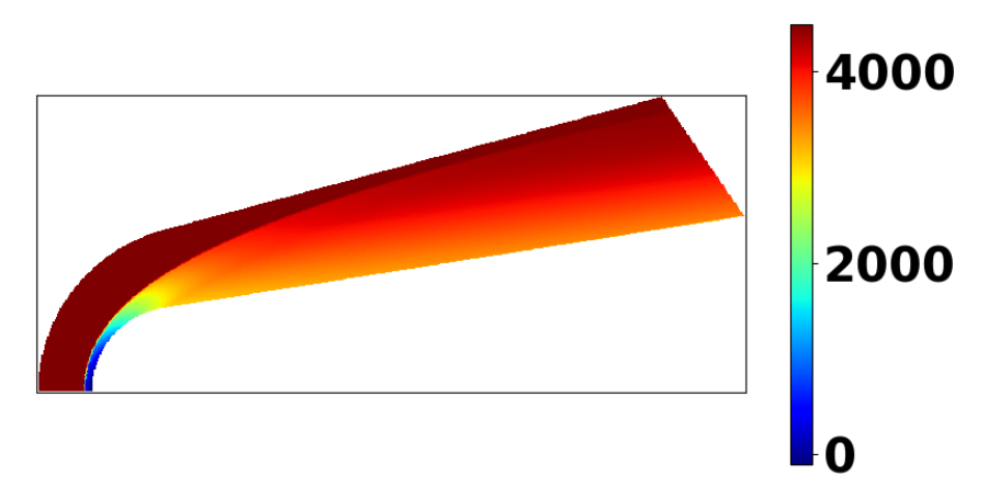
(a)

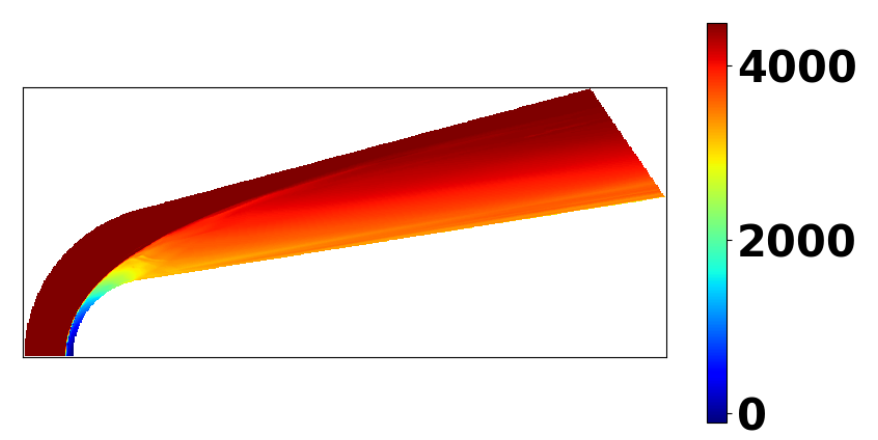
(b)

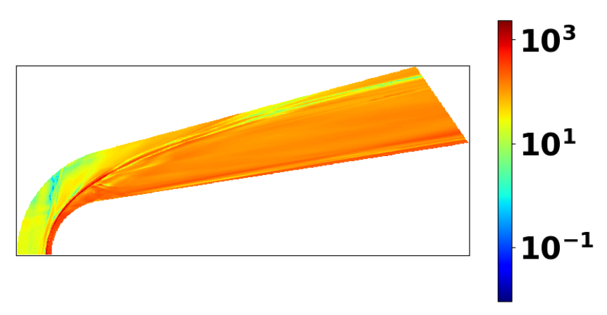
(c)

Figure 2: $x$-velocity $u_{1}$ at Mach $15$ and altitude $26\text{\,}\mathrm{k}\mathrm{m}$ predicted by NBF on evaluation data.

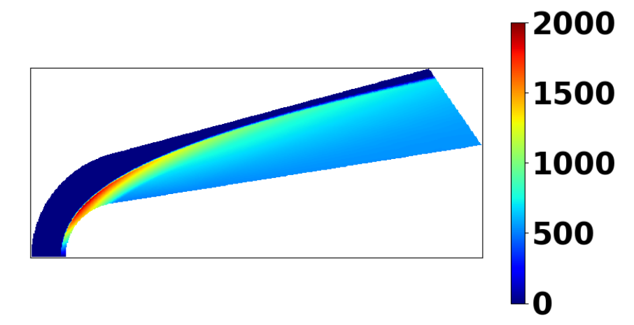
(a)

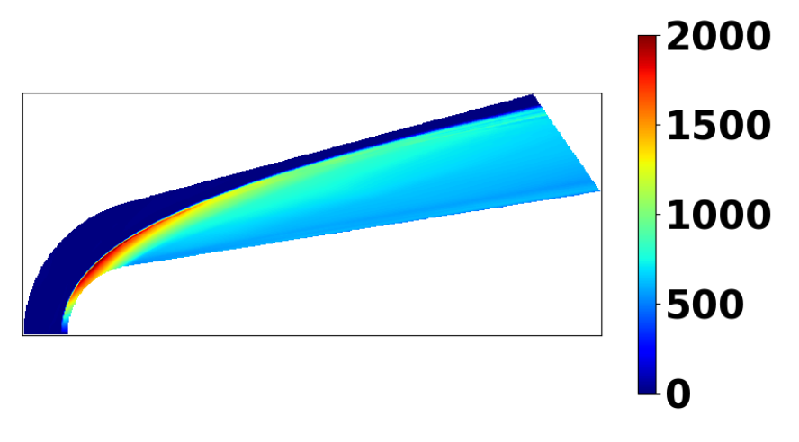
(b)

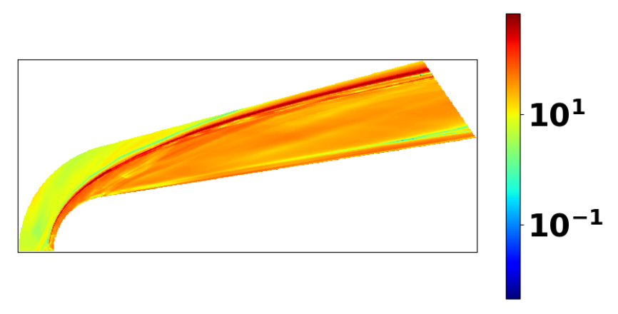
(c)

Figure 3: The $y$-velocity $u_{2}$ at Mach $15$ and altitude $26\text{\,}\mathrm{k}\mathrm{m}$, predicted by NBF on evaluation data.

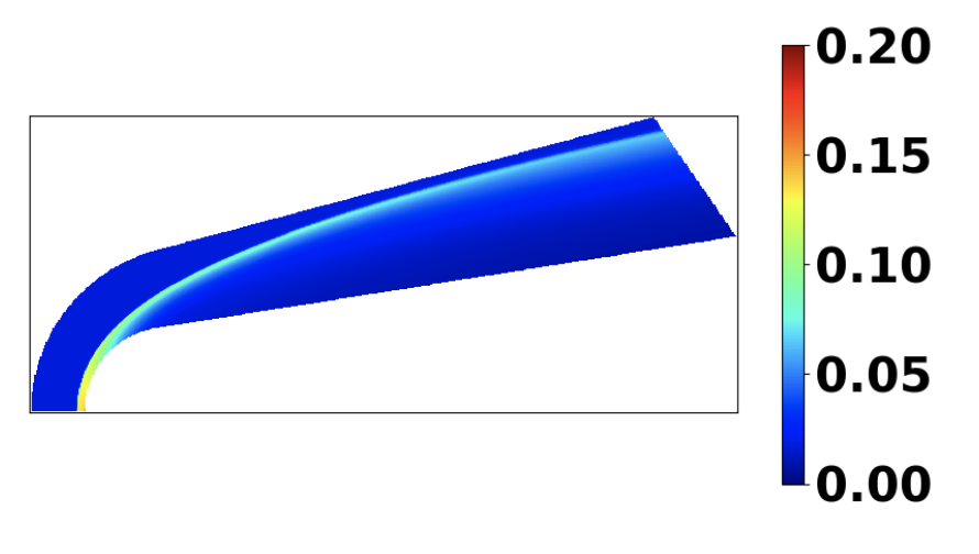
(a)

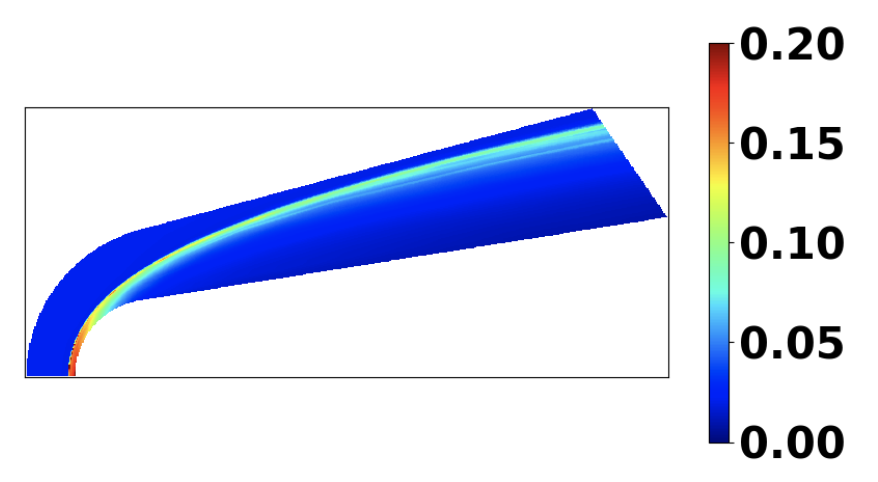
(b)

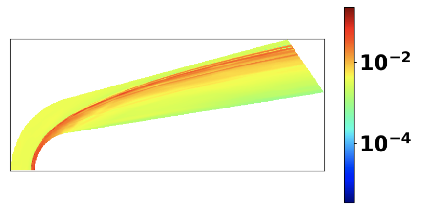
(c)

Figure 4: Density $\rho$ at Mach $15$ and altitude $26\text{\,}\mathrm{k}\mathrm{m}$, predicted by NBF on evaluation data.

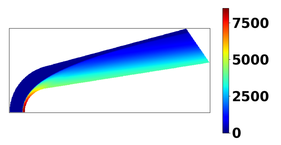
(a)

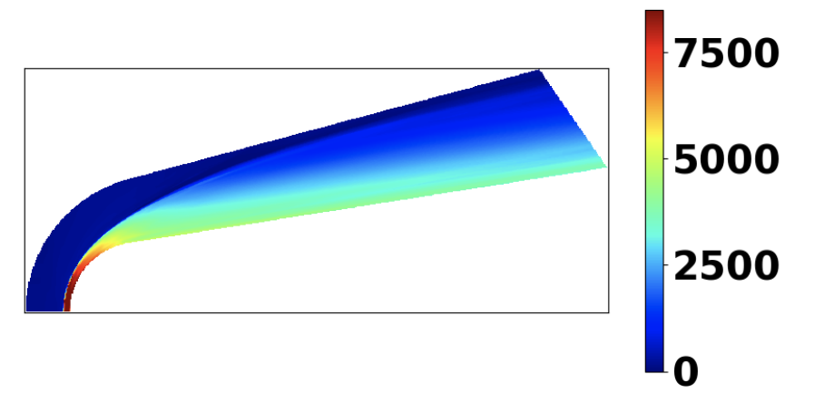
(b)

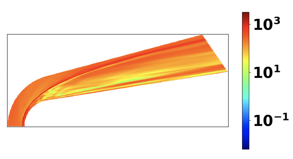
(c)

Figure 5: Temperature $T$ at Mach $15$ and altitude $26\text{\,}\mathrm{k}\mathrm{m}$, predicted by NBF on evaluation data.

It is also informative to assess how well the models fit the training data, which we show in Table 2. The NBF has significantly lower errors as compared to the DeepONet. However, fitting the RAM-C II data remains challenging for both SciML models, particularly for $\rho$. Even on the training set, no model surpasses relative error of $0.01$, and error for density $\rho$ remains high, at least $0.4$. Potential mitigation strategies include larger and more expressive models and more precise optimization strategies that include more than first-order derivative information (e.g., (20; 21; 22)).

Model	$u_{1}$ error (std)	$u_{2}$ error (std)	$\rho$ error (std)	$T$ error (std)
DeepONet	0.0567 (0.0162)	0.2154 (0.0284)	0.704 (0.159)	0.382 (0.0799)
NBF	0.0361 (0.00217)	0.0803 (0.0184)	0.450 (0.138)	0.107 (0.0260)

Table 2: Model training fit: We report the data errors for our models with each state variable’s relative error, averaged over all the configurations in the train split.

4 Conclusion

This paper demonstrates that a modified version of the NBF is able to accurately predict hypersonic fluid flow on a dataset of over 200 parameter values after training on just 10 data fields. The NBF method is able to predict the data fields in the validation set at a much higher accuracy than DeepONet.

The NBF method can be used to model complex fluid flow in scenarios that only have a small amount of data. By improving the applicability of data-driven models for fluid flow, NBFs can be used to advance prediction, allowing for a faster engineering design process.

Appendix A Data generation

We solve the compressible steady-state NSE (Appendix C) on a two-dimensional domain. Specifically, we simulate high Mach number flow over a blunt nose cone. This academic problem is based on a series of experiments that were performed in the 1960s: the RAM flight experiments. These were designed to study plasma, specifically its effect on communication blackout during reentry. At high hypersonic Mach numbers, the temperatures surrounding the vehicle become sufficiently high that gas dissociates and ionizes, forming a thin plasma layer around the vehicle. The ionized air blocks out the incoming radio signal, causing communication blackout.

The configuration of our study is based on the second flight test (RAM-C II). The RAM-C II vehicle can nominally be represented by a spherical blunt nose cone (Figure 1a). The nose radius is $0.1524\text{\,}\mathrm{m}$ and connects tangentially to the cone body, which has a half-cone angle of $9\text{\,}{}^{\circ}$. The full body length of the configuration is $1.3\text{\,}\mathrm{m}$.

Because the configuration is axisymmetric, we can simulate the system in two dimensions. Figure 1b displays an example of the domain mesh along with its four boundaries (inflow, symmetry, cone wall and outflow). The inflow boundary is a Dirichlet boundary condition (BC), and a Neumann BC was used for the outflow. The symmetry line is a Neumman BC for all its variables except for velocity component normal to the boundary; this component was forced to vanish at the boundary. The wall uses a mixed set of BCs: the velocity is forced to vanish at the wall, the temperature is forced to equal $1200\text{\,}\mathrm{K}$, and the Neumann BC is applied to the remaining dependent variables. For initializing the solver, the whole domain uses same condition as the inflow boundary.

To generate the training dataset, computational fluid dynamics (CFD) solutions were collected for various altitudes and Mach numbers. The CFD solver was used to solve the single species (air) NSE. The solution inputs were parameterized by altitude and Mach number. Altitudes covered values of $20\text{\,}\mathrm{k}\mathrm{m}$ to $60\text{\,}\mathrm{k}\mathrm{m}$ in increments of $2\text{\,}\mathrm{k}\mathrm{m}$. Mach numbers covered values of $10$ to $30$ in increments of $1$. In total, $441$ solutions were generated.

CFD++ version 20.1 [23] was utilized to perform all the simulations. CFD++ is an unstructured finite volume flow solver that is maintained by Metacomp Technologies Inc. It has the capability of solving the full Navier-Stokes equations with high-order spatial and temporal accuracy. To solve the single species Navier-Stokes equations, the solver uses a pseudo time marching approach. The initial condition is integrated over time until convergence is reached at which point we have our steady-state solution. Additional details on CFD++ can be found in the user manual [24].

Appendix B Network hyperparameters

Table 3 and Table 4 give the hyperparameters used to train the NBF and DeepONet models. They were chosen based on experimentation with a similar RAM-C II dataset that used different configuration parameters and mesh points.

Hyperparameter	Value
# of hidden units for each basis function $\phi_{j,\ell}$	$40$
# of layers for each basis function $\phi_{j,\ell}$	$7$
# of hidden units for each unknowns function $C_{j,\ell}$	$100$
# of layers for each unknowns function $C_{j,\ell}$	$7$
# of hidden units for each nonlinear function $f_{\text{nonlin},\ell}$	$7$
# of layers for each nonlinear function $f_{\text{nonlin},\ell}$	$100$
# epochs to train the basis functions	$100$
learning rate for training the basis functions	$10^{-3}$
# steps to decrease the learning rate for the basis functions	$45$
learning rate reduction factor $\gamma$ for the basis functions	$0.9$
# epochs to pretrain the NBF	$10000$
learning rate for training the basis functions	$10^{-3}$
# steps to decrease the learning rate for pretraining	$800$
learning rate reduction factor $\gamma$ for pretraining	$0.9$
# epochs to train the NBF	$1$
learning rate for training the NBF	$10^{-3}$
# steps to decrease the learning rate for the NBF	$8$
learning rate reduction factor $\gamma$ for the NBF	$0.1$

Table 3: Hyperparameters for training the NBF models (Eq. 2)

Hyperparameter	Value
# of hidden units for the spatial encoder $f_{x}$	$32$
# of layers for the spatial encoder $f_{x}$	$1$
# of hidden units for the parameter encode $f_{\psi}$	$32$
# of layers for the parameter encoder $f_{\psi}$	$1$
# of hidden units for the decoder $f_{d}$	$256$
# of layers for the decoder $f_{d}$	$3$
weight decay for training the DeepONets	$10^{-4}$
# epochs for training the DeepONets	$97$

Table 4: Hyperparameters for training the DeepONet models (Eq. 1)

Appendix C Governing equations

The four state variables of interest are $w=[u_{1},u_{2},\rho,T]$, where $u_{1}$ and $u_{2}$ are the velocities in the $x_{1}$ and $x_{2}$ directions, $\rho$ is the density, and $T$ is the temperature. The state variables obey the following compressible single-gas NSE:

$$\sum_{j}\partial_{x_{j}}\left(\rho u_{j}\right) = 0\,\,\,\,\,(\text{continuity})$$ (5)

$$\sum_{j}\partial_{x_{j}}\left(\rho u_{i}u_{j}+p\delta_{ij}\right) = \sum_{j}\partial_{j}\tau_{ij},\,\,\,\,i=1,2,\,\,\,(\text{momentum-conservation})$$ (6)

$$\partial_{j}\partial_{j}\left[(E+p)u_{j}\right] = \sum_{j}\left[\sum_{i}\tau_{ij}u_{i}-k\partial_{x_{j}}T\right],\,\,\,(\text{energy-conservation)}.$$ (7)

Here, $E$ is the energy, given by $E=e+\frac{1}{2}\rho\sum_{i}u_{i}u_{i}$. The specific sensible enthalpy ($h$) satisfies the relations $h=e+RT$. The thermodynamic properties are modeled as polynomial-based function of temperature. For our case,

$$h = R\left(a_{1}+\frac{a_{2}}{2}T+\frac{a_{3}}{3}T^{2}+\frac{a_{4}}{4}T^{3}+\frac{a_{5}}{5}T^{4}\right)T+\Delta h_{f}^{0},$$ (8)

where the polynomial coefficients $a_{1},a_{2},a_{3},a_{4},a_{5}$ are determined empirically. For this study, we use a simplified model for air where $a_{1}\neq 0$ and $a_{2}=a_{3}=a_{4}=a_{5}=\Delta h_{f}^{0}=0$ ; thus, $h=Ra_{1}T$. Viscous stress tensor ($\tau$) and strain rate tensor ($S$) are defined as following,

$$S_{ij} = \frac{1}{2}\left(\partial_{x_{j}}u_{i}+\partial_{x_{i}}u_{j}\right),\,\,\,\,i,j=1,2$$ (9)

$$\tau_{jj} = 2\mu\left(S_{jj}-\frac{1}{3}\sum_{i}S_{ii}\right),\,\,\,\,j=1,2$$ (10)

$$\tau_{ij} = 2\mu S_{ij},\,\,\,\,i\neq j,$$ (11)

and viscosity ($\mu$) and thermal conductivity ($k$) are defined by Sutherland’s model:

$$\frac{\mu}{\mu_{0}} = \left(\frac{T}{T_{0,\mu}}\right)^{3/2}\frac{T_{0,\mu}+S_{\mu}}{T+S_{\mu}}$$ (12)

$$\frac{k}{k_{0}} = \left(\frac{T}{T_{0,k}}\right)^{3/2}\frac{T_{0,k}+S_{k}}{T+S_{k}},$$ (13)

and $R$, $a_{1}$, $\mu_{0}$, $T_{0,\mu}$, $S_{\mu}$, $k_{0}$, $T_{0,k}$, and $S_{k}$ are constant parameters given in Table 5.

Parameter	Name	Value
$R$	Specific gas constant	$287\text{\,}\frac{J}{Kg\cdot K}$
$a_{1}$	Polynomial coefficient	$3.5$
$\mu_{0}$	Viscosity at reference temperature	$1.716\text{\times}{10}^{-5}\text{\,}\frac{kg}{m\cdot s}$
$T_{0,\mu}$	Reference temperature for viscosity	$273.11\text{\,}\mathrm{K}$
$S_{\mu}$	Sutherland constant for viscosity	$111K$
$k_{0}$	Thermal conductivity at reference temperature	$2.41\text{\times}{10}^{-2}\text{\,}\frac{W}{m\cdot K}$
$T_{0,k}$	Reference temperature for thermal conductivity	$273.11\text{\,}\mathrm{K}$
$S_{k}$	Sutherland constant for thermal conductivity	$194\text{\,}\mathrm{K}$

Table 5: NSE parameters used to generate training and evaluation data

References

- [1] E. Vendel, V. Rottschäfer, and E. C. M. de Lange. Improving the prediction of local drug distribution profiles in the brain with a new 2d mathematical model. Bulletin of Mathematical Biology, 81(9):3477–3507, Sep 2019.
- [2] Noah Ford and David Chopp. A dimensionally reduced model of biofilm growth within a flow cell. Bulletin of Mathematical Biology, 82(3):40, Mar 2020.
- [3] Xiaowei Jin, Shengze Cai, Hui Li, and George Em Karniadakis. NSFnets (Navier-Stokes Flow Nets): Physics-informed Neural Networks for the Incompressible Navier-Stokes Equations. Journal of Computational Physics, 426:109951, 2021.
- [4] George Em Karniadakis, Ioannis G Kevrekidis, Lu Lu, Paris Perdikaris, Sifan Wang, and Liu Yang. Physics-Informed Machine Learning. Nature Reviews Physics, 3(6):422–440, 2021.
- [5] Sifan Wang, Hanwen Wang, and Paris Perdikaris. Learning the solution operator of parametric partial differential equations with physics-informed deeponets. Science Advances, 7(40):eabi8605, 2021.
- [6] Sifan Wang and Paris Perdikaris. Long-time integration of parametric evolution equations with physics-informed deeponets. Journal of Computational Physics, 475:111855, 2023.
- [7] Zongyi Li, Hongkai Zheng, Nikola B. Kovachki, David Jin, Haoxuan Chen, Burigede Liu, Kamyar Azizzadenesheli, and Anima Anandkumar. Physics-informed neural operator for learning partial differential equations. CoRR, abs/2111.03794, 2021.
- [8] Lu Lu, Xuhui Meng, Shengze Cai, Zhiping Mao, Somdatta Goswami, Zhongqiang Zhang, and George Em Karniadakis. A comprehensive and fair comparison of two neural operators (with practical extensions) based on fair data. Computer Methods in Applied Mechanics and Engineering, 393:114778, 2022.
- [9] David Witman, Alexander New, Hicham Alkandry, and Honest Mrema. Neural basis functions for accelerating solutions to high mach euler equations. In ICML 2022 2nd AI for Science Workshop, 2022.
- [10] Lu Lu, Pengzhan Jin, Guofei Pang, Zhongqiang Zhang, and George Em Karniadakis. Learning nonlinear operators via deeponet based on the universal approximation theorem of operators. Nature Machine Intelligence, 3(3):218–229, Mar 2021.
- [11] Lawrence Sirovich. Turbulence and the dynamics of coherent structures. i. coherent structures. Quarterly of applied mathematics, 45(3):561–571, 1987.
- [12] Erin Farbar, Iain D. Boyd, and Alexandre Martin. Numerical prediction of hypersonic flowfields including effects of electron translational nonequilibrium. Journal of Thermophysics and Heat Transfer, 27(4):593–606, 2013.
- [13] Pawel Sawicki, Ross S. Chaudhry, and Iain D. Boyd. Influence of chemical kinetics models on plasma generation in hypersonic flight. In AIAA Scitech 2021 Forum, 2021.
- [14] Diederik P. Kingma and Jimmy Ba. Adam: A Method for Stochastic Optimization, 2014. doi:10.48550/ARXIV.1412.6980.
- [15] Adam Paszke, Sam Gross, Francisco Massa, Adam Lerer, James Bradbury, Gregory Chanan, Trevor Killeen, Zeming Lin, Natalia Gimelshein, Luca Antiga, Alban Desmaison, Andreas Kopf, Edward Yang, Zachary DeVito, Martin Raison, Alykhan Tejani, Sasank Chilamkurthy, Benoit Steiner, Lu Fang, Junjie Bai, and Soumith Chintala. Pytorch: An imperative style, high-performance deep learning library. In Advances in Neural Information Processing Systems 32, pages 8024–8035. Curran Associates, Inc., 2019.
- [16] Lu Lu, Xuhui Meng, Zhiping Mao, and George Em Karniadakis. Deepxde: A deep learning library for solving differential equations. SIAM Review, 63(1):208–228, 2021.
- [17] Sifan Wang, Yujun Teng, and Paris Perdikaris. Understanding and Mitigating Gradient Flow Pathologies in Physics-Informed Neural Networks. SIAM Journal on Scientific Computing, 43(5):A3055–A3081, 2021.
- [18] Aditi Krishnapriyan, Amir Gholami, Shandian Zhe, Robert Kirby, and Michael W Mahoney. Characterizing Possible Failure Modes in Physics-Informed Neural Networks. Advances Neural Inf. Process. Syst., 34, 2021.
- [19] Alexander New, Benjamin Eng, Andrea C. Timm, and Andrew S. Gearhart. Tunable complexity benchmarks for evaluating physics-informed neural networks on coupled ordinary differential equations. In 2023 57th Annual Conference on Information Sciences and Systems (CISS), pages 1–8, 2023.
- [20] R. H. Byrd, S. L. Hansen, Jorge Nocedal, and Y. Singer. A stochastic quasi-newton method for large-scale optimization. SIAM Journal on Optimization, 26(2):1008–1031, 2016.
- [21] Zhewei Yao, Amir Gholami, Sheng Shen, Mustafa Mustafa, Kurt Keutzer, and Michael Mahoney. Adahessian: An adaptive second order optimizer for machine learning. Proceedings of the AAAI Conference on Artificial Intelligence, 35(12):10665–10673, May 2021.
- [22] Ehsan Amid, Rohan Anil, and Manfred Warmuth. Locoprop: Enhancing backprop via local loss optimization. In Gustau Camps-Valls, Francisco J. R. Ruiz, and Isabel Valera, editors, Proceedings of The 25th International Conference on Artificial Intelligence and Statistics, volume 151 of Proceedings of Machine Learning Research, pages 9626–9642. PMLR, 28–30 Mar 2022.
- [23] MultiMedia LLC. CFD++, Version 20.1, 2023.
- [24] CFD++ and CAA++ User Manual Version 11.1.