Optimal minimax rate of learning interaction kernels

Abstract

Nonparametric estimation of nonlocal interaction kernels is crucial in various applications involving interacting particle systems. The inference challenge, situated at the nexus of statistical learning and inverse problems, comes from the nonlocal dependency. A central question is whether the optimal minimax rate of convergence for this problem aligns with the rate of $M^{-\frac{2\beta}{2\beta+1}}$ in classical nonparametric regression, where $M$ is the sample size and $\beta$ represents the smoothness exponent of the radial kernel. Our study confirms this alignment for systems with a finite number of particles.

We introduce a tamed least squares estimator (tLSE) that attains the optimal convergence rate for a broad class of exchangeable distributions. The tLSE bridges the smallest eigenvalue of random matrices and Sobolev embedding. This estimator relies on nonasymptotic estimates for the left tail probability of the smallest eigenvalue of the normal matrix. The lower minimax rate is derived using the Fano-Tsybakov hypothesis testing method. Our findings reveal that provided the inverse problem in the large sample limit satisfies a coercivity condition, the left tail probability does not alter the bias-variance tradeoff, and the optimal minimax rate remains intact. Our tLSE method offers a straightforward approach for establishing the optimal minimax rate for models with either local or nonlocal dependency.

Keywords: Nonparametric regression; interacting particle systems; optimal minimax rate; tamed least squares estimator; random matrices

Mathematics Subject Classification: Primary 62G08; secondary 62G20, 60B20

1 Introduction

Consider the nonparametric regression of the radial interaction kernel $\phi:\mathbb{R}^{+}\to\mathbb{R}$ in the model

$$Y=R_{\phi}[X]+\eta,$$ (1.1)

from data consisting of samples $\{(X^{m},Y^{m})\}_{m=1}^{M}$ of the joint distribution of $(X,Y)$. Here $Y$ and $X$ are ${\mathbb{R}}^{N\times d}$-valued random variables with $N\geq 3$, denoted by $Y=(Y_{1},\ldots,Y_{N})^{\top}$ and $X=(X_{1},\ldots,X_{N})^{\top}$. The operator $R_{\phi}[X]=(R_{\phi}[X]_{1},\cdots,R_{\phi}[X]_{N})^{\top}$ represents the interaction between particles through the kernel $\phi$, its entries are defined by

$$R_{\phi}[X]_{i}=\frac{1}{N}\sum_{j\neq i}\phi(|X_{i}-X_{j}|)\frac{X_{i}-X_{j}}{|X_{i}-X_{j}|},\quad i=1,\ldots\,N\,,.$$ (1.2)

where we write $\sum_{j\neq i}:=\sum_{j=1,j\neq i}^{N}$ in short. The noise $\eta$ in the model is independent of $X$ and not necessarily Gaussian.

Nonparametric regression is particularly suitable for estimating the kernel $\phi$, thanks to the linear dependence of $R_{\phi}$ on $\phi$. A regression estimator is the minimizer of an empirical mean-square loss function

$$\mathcal{E}_{M}(\phi)=\sum_{m=1}^{M}\frac{1}{N}\|Y^{m}-R_{\phi}[X^{m}]\|_{\mathbb{R}^{Nd}}^{2}\,$$ (1.3)

over a hypothesis space that is adaptively chosen to avoid underfitting and overfitting.

The above nonparametric regression problem arises in the inference for systems of interacting particles or agents. Such systems are prevalent in collective dynamics in various fields, including flocking [CS07, AH10, CDP18], opinion dynamics [MT14], kinetic granular media [CMV03, CGM07], to name just a few. Driven by the applications, the past decade sees a burst of efforts on inferring the system from data, including parametric [DMH23, MB22, LQ22], semi-parametric [BPP23], and nonparametric [DMH22, YCY22, LZTM19, LMT21] approaches. Given often limited prior knowledge about the kernel in applications, a nonparametric approach is desirable. In particular, the studies [LZTM19, LMT21, LMT22] consider nonparametric inference of radial interaction kernels for first-order stochastic differential equations in the form

$$\mathrm{d}X(t)=R_{\phi}[X(t)]\mathrm{d}t+\sigma\mathrm{d}B(t)\,,$$ (1.4)

where $X(t)=(X_{1}(t),\cdots,X_{N}(t))$ represents the position of particles, $R_{\phi}$ is same as in (1.2) and $B(t)$ is a standard Brownian motion in $\mathbb{R}^{Nd}$ with $\sigma\geq 0$ representing the scale of the random noise. The least squares estimator is demonstrated to exhibit a convergence rate of $\big{(}\frac{M}{\log M}\big{)}^{-\frac{2\beta}{2\beta+1}}$, where $M$ is the number of independent trajectories and $\beta\geq 1$ represents the Hölder exponent of the true kernel. However, the optimal minimax rate, namely the best convergence rate in the worst case, remains open.

This study aims to answer the optimal minimax rate question. We consider the simplified but generic statistical model (1.1), which rules out the numerical error from the discretization of the differential equations and the dependence between the components in trajectory data.

1.1 Main results

This study establishes that the rate of $M^{-\frac{2\beta}{2\beta+1}}$ is the optimal minimax rate of convergence under a coercivity condition that ensures the well-posedness of the inverse problem in the large sample limit. Informally, we establish the following minimax rate:

$$\inf_{\widehat{\phi}_{M}}\sup_{\phi_{*}\in\mathcal{H}(\beta)}\mathbb{E}[\|\widehat{\phi}_{M}-\phi_{*}\|_{L^{2}_{\rho}}^{2}]\approx M^{-\frac{2\beta}{2\beta+1}}\,,\quad\text{ as }M\to\infty,$$

where the infimum is among all estimators $\widehat{\phi}_{M}$ inferred from data, and the hypothesis space $\mathcal{H}(\beta)$ can be a Sobolev class $W(\beta,L)$ or Hölder class $\mathcal{C}(\beta,L)$ in Definitions 2.13–2.14). Importantly, the rate also holds for the case $\beta\leq 1/2$, which contains discontinuous functions. The space $L^{2}_{\rho}$ is the space of square-integrable functions under the weight $\rho$, which is the probability measure of pairwise distances.

A major innovation of our study is a new approach to prove the upper minimax rate. We introduce a tamed least square estimator (tLSE) in Definition 3.1 and show that it achieves the optimal rate with a straightforward proof. The proof is based on non-asymptotic estimates of the left tail probability of the smallest eigenvalue of the normal matrix; see Theorem 3.6 and the subsequent discussion on technical innovations.

To affirm that the upper minimax rate is optimal, we prove in Theorem 4.1 that the rate is also the lower minimax rate. We accomplish this by applying the Fano-Tsybakov method in [Tsy08], which we generalize to include the weight measure $\rho$. This involves careful construction of hypothesis functions for hypothesis testing in Section 4.

1.2 Main difficulties and technical innovations

The optimal minimax rate is well-established for classical nonparametric estimation (see, e.g., [CS02b, GKKW06, Tsy08] and the reference therein). In this classical setting, one estimates the function $\phi:\mathbb{R}\to\mathbb{R}$ in the model $Y=\phi(Z)+\eta$ from sample data $\{(Z^{m},Y^{m})\}_{m=1}^{M}$, where the data $Y$ depends on locally on a single value of $\phi$. A critical fact in this setting is that the conditional expectation $\phi(z)=\mathbb{E}[Y|Z=z]$ uniquely minimizes the large sample limit of the empirical squared loss, leading to a well-posed inverse problem. Notable estimators achieving the minimax rate include the projection estimator for deterministic $Z$ data (see e.g., [Tsy08]), and the least squares estimator for random $Z$ using tools from the empirical process theory, which are based on covering arguments with the chaining technique (see e.g., [VdV00] and [GKKW06, Chapter 19]).

However, nonlocal dependance presents a new challenge in interaction kernel estimation. The nonlocal dependence means that the operator $R_{\phi}[X]$ depends on the kernel $\phi$ non-locally through the weighted sum of multiple values of $\phi$, similar to a convolution. Thus, this intersection of statistical learning and deconvolution-type inverse problems raises significant hurdles in both well-posedness and constructing estimators achieving the minimax rate.

To address these challenges, we show first that the inverse problem is well-posed for a large class of distributions of $X$ satisfying Assumption 2.1. A key condition for well-posedness is the coercivity condition, which is both necessary and sufficient([LZTM19, LMT22, LLM⁺21]). This condition also implies the uniform convexity of the expected loss function in $L^{2}_{\rho}$, as shown in Proposition 2.8. Due to these specifics, a universal convergence rate for all distributions is not feasible.

Our major technical innovation lies in developing the tamed least square estimator with straightforward proof. The tLSE is zero when the minimal eigenvalue of the normal matrix is below a threshold, and it is the least squares estimator otherwise. That is,

$$\widehat{\phi}_{n,M}^{tlse}=\sum_{k=1}^{n}\theta_{k}^{tlse}\psi_{k},\quad\text{ where }(\theta_{1}^{tlse},\ldots,\theta_{n}^{tlse})^{\top} =[\widebar{\mathbf{A}}_{n}^{M}]^{-1}\widebar{\mathbf{b}}_{n}^{M}\mathbf{1}_{\{\lambda_{\min}(\widebar{\mathbf{A}}_{n}^{M})>\frac{1}{4}c_{\bar{\mathcal{L}}}\}}\,,$$ (1.5)

where the threshold $c_{\bar{\mathcal{L}}}$ is the coercivity constant in Definition 2.6. Here $\widebar{\mathbf{A}}_{n}^{M}$ and $\widebar{\mathbf{b}}_{n}^{M}$ are the normal matrix and norm vector for the regression over the hypothesis space $\mathcal{H}_{n}=\mathrm{span}\{\psi_{k}\}_{k=1}^{n}$ with orthonormal basis functions $\psi_{k}$. Note that only in the set $\{\lambda_{\min}(\widebar{\mathbf{A}}_{n}^{M})<\frac{1}{4}c_{\bar{\mathcal{L}}}\}$, the tLSE differs from the least squares estimator

$$(\theta_{1}^{lse},\ldots,\theta_{n}^{lse})^{\top}=[\widebar{\mathbf{A}}_{n}^{M}]^{\dagger}\widebar{\mathbf{b}}_{n}^{M},$$

where $[\widebar{\mathbf{A}}_{n}^{M}]^{\dagger}$ denotes the Moore-Penrose inverse of $\widebar{\mathbf{A}}_{n}^{M}$. A crucial observation in our proof is that the optimal minimax rate is attained if the probability of the set $\{\lambda_{\min}(\widebar{\mathbf{A}}_{n}^{M})<\frac{1}{4}c_{\bar{\mathcal{L}}}\}$ does not affect the bias-variance tradeoff. This leads to the study of the left tail probability of $\lambda_{min}(\widebar{\mathbf{A}}_{n}^{M})$ with the dimension $n\approx M^{\frac{1}{2\beta+1}}$ chosen from the tradeoff, aiming for a non-asymptotic bound exponentially decaying in $M$.

We establish two non-asymptotic estimates for the left tail probability of the smallest eigenvalue of the normal matrix. Lemma 3.11 shows that with the coercivity condition alone and an application of the Bernstein’s inequality for random matrices, we have

$$\mathbb{P}\left\{\lambda_{\min}(\bar{\mathbf{A}}_{n}^{M})\leq(1-\varepsilon)c_{\bar{\mathcal{L}}}\right\}\leq 2n\exp\left(-\frac{c_{1}\varepsilon^{2}M}{c_{2}n^{2}+c_{3}\varepsilon}\right)\,,\forall\varepsilon\in(0,1),$$

where $c_{1},c_{2},c_{3}$ are positive constants universal for $\varepsilon$, $n$ and $M$. This estimate enables a simple proof of the minimax rate for the tLSE when the true function has a smoothness exponent $\beta>1/2$. We also extend the optimal rate to $\beta\leq 1/2$, under an additional assumption on the fourth moment of $R_{\phi}[X]$ in Assumption 2.17. This extension relies on an improved bound for the left tail probability of the smallest eigenvalue in Lemma 3.12:

$$\mathbb{P}\left\{\lambda_{\min}(\bar{\mathbf{A}}_{n}^{M})\leq\frac{1-\varepsilon}{2}c_{\bar{\mathcal{L}}}\right\}\leq\exp\left(c_{4}n-c_{5}\varepsilon^{2}M\right)\,,\forall\varepsilon\in(0,1),$$

where $c_{4},c_{5}$ are positive constants universal for $n$ and $M$. The primary tool is the PAC-Bayes inequality introduced in [Oli16, Mou22] to analyze the left tail of random matrices. We note that our fourth-moment assumption on $R_{\phi}[X]$ is an extension to the function space setting from a fourth-moment assumption on covariance matrices in [Oli16, Mou22]. Notably, this assumption is supported by fractional Sobolev embedding theorems when $\beta\geq 1/4$, as elaborated in Remark 2.18. It remains open to study the case $\beta\in(0,1/4)$, which we discuss in Section 3.4.

Table 1 summarizes these left tail probabilities and their applicable range of $\beta$ in the minimax rate.

Table 1: The left tail probability bounds and applicable range of $\beta$ in the minimax rate.

Left tail probability	Method	Assumptions	Range of $\beta$
$n\exp\left(-\frac{c_{1}\varepsilon^{2}M}{c_{2}n^{2}+c_{3}\varepsilon}\right)$	Bernstein’s Ineq.	Assum. 2.12	$\beta>1/2$
$\exp\left(c_{4}n-c_{5}\varepsilon^{2}M\right)$	PAC-Bayes Ineq.	Assum. 2.12 and 2.17	$\beta\geq 1/4$

1.3 Summary of main contributions and insights

This study makes contributions in two key parts:

1. Optimal rate of convergence for interaction kernel learning. We have established the optimal convergence rate $M^{-\frac{2\beta}{2\beta+1}}$ for learning the interaction kernel in Model (1.1) across a wide range of distributions. Moreover, this optimal rate of $M^{-\frac{2\beta}{2\beta+1}}$ applies to Sobolev classes with $\beta\leq\frac{1}{2}$. This encompasses widely used discontinuous functions such as piecewise constant functions.

2. Introduction of the Tamed Least Square Estimator (tLSE): The tLSE represents a new and efficient method for proving the minimax rate in nonparametric regression. A key insight is that the optimal minimax rate depends on whether the bias-variance tradeoff can remain unaffected by the left tail probability of the smallest eigenvalue of the normal matrix. This revelation is crucial for advancement in our understanding of nonparametric regression. It establishes a connection between the minimax rate, the left tail probability of the smallest eigenvalue of the random normal matrix, and fractional Sobolev embedding.

The insights gained from this study pave the way for future research on the minimax rate for nonparametric regression regarding models with nonlocal dependence. The inverse problem in the large sample limit plays a fundamental role. We’ve focused on scenarios where the inverse problem is well-posed, finding that the optimal minimax rate $M^{-\frac{2\beta}{2\beta+1}}$ is consistent for regression with both local and nonlocal dependencies. In contrast, when the inverse problem is ill-posed, i.e., with a zero coercivity constant, the optimal rate, if it exists, is expected to be slower than $M^{-\frac{2\beta}{2\beta+1}}$ since the current rate bears a constant depending on the reciprocal of the coercivity constant. Thus, exploring the convergence rate without the coercivity condition remains an open and intriguing area for further investigation.

Additionally, our study has centered on convergence in the sample size $M$ while keeping the number of particles $N$ finite. An intriguing direction for future research lies in examining the convergence rate as $N$ increases. Given that the inverse problem becomes an ill-posed deconvolution in the limit of $N=\infty$, we conjecture that the convergence rate will be slower than $N^{-\frac{2\beta}{2\beta+1}}$ and may depend on the spectrum of the normal operator.

1.4 Related work

Minimax rate for nonparametric regression.

The study of the minimax rate in nonparametric regression is a well-established and extensively explored topic within inference and learning. Due to the vastness of the literature, we direct readers to [GKKW06, Tsy08, CS02b, NR19], among others, for comprehensive reviews. For lower minimax rates, this study utilizes the Fano-Tsybakov hypothesis testing method [Tsy08], although alternatives like the van Trees method [GL95] are also viable.

For the upper minimax rate, notable estimators achieving the optimal rate without the logarithmic term include the projection estimator for deterministic input data (see, e.g., [Tsy08]), and the least squares estimator whose rate is proved by using the empirical process theory with covering arguments and chaining technique (see, e.g., [VdV00] and [GKKW06, Chapter 19]). Additionally, we note that the empirical process theory with a covering argument is widely used, and it applies to the interaction kernel estimation (see, e.g., [LZTM19, LMT22, LMT21]). However, it leads to a sub-optimal rate with a logarithmic factor when using a fixed cover. The chaining technique may remove the logarithmic factor by constructing a sequence of covers and additional assumptions, but the nonlocal dependence will further complicate the proof. Our tamed least square estimator (tLSE) stands out for its simplicity and broad applicability to nonparametric regression problems with either local or nonlocal dependencies.

Inference for systems of interacting particles.

A large amount of literature has been devoted to the inference for systems of interacting particles, and we can only sample a few here. Parametric inference has been studied in [DMH23, SKPP21, AHPP23, LQ22, Kas90, Che21] for the drift and in [HLL19] for the diffusion. Nonparametric inference on estimating the drift $R_{\phi}$, but not the kernel $\phi$, has been studied in [YCY22, DMH22]. The semi-parametric inference in [BPP23] estimates the interaction kernel. All these studies consider the case when $N\to\infty$ from a single long trajectory of the system. Inference of the mean-field equations has also been studied in [MB22, MTB22, LL22, DMH22]. The closest to this study are [LZTM19, LMT21, LMT22], where the rate for learning the interaction kernels from multiple trajectories is $\big{(}\frac{M}{\log M}\big{)}^{-\frac{2\beta}{2\beta+1}}$, is suboptimal due to the use of supremum norm in the covering number argument. Building on these results, our study achieves the optimal rate in a simplified static model (1.1), advancing the understanding of the inference problem.

Nonparametric deconvolution.

Nonlocal dependence is a key feature in nonparametric deconvolution, particularly in estimating probability densities as studied in [Fan91, Mei09], among others. In such contexts, the underlying inverse problem in the large sample limit typically manifests as an ill-posed deconvolution challenge. The established optimal rate for these scenarios is $M^{-\frac{2\beta}{2\beta+2\alpha+1}}$, where $\alpha$ is the decay rate of the Fourier transform’s derivative of the convolution kernel. In contrast, our study navigates a well-posed inverse problem made possible through the coercivity condition, differentiating it from the typical deconvolution framework.

Linear regression for parametric inference and random matrices.

The normal matrix $\widebar{\mathbf{A}}_{n}^{M}$ in our study resembles the sample covariance matrix $\frac{1}{M}\sum_{m=1}^{M}x^{m}(x^{m})^{\top}$ in linear regression $y\approx\bm{\theta}^{\top}x$ from samples $\{(x^{m},y^{m})\}$ of a distribution on $\mathbb{R}^{n}\times\mathbb{R}$. Therefore, the analysis of this normal matrix can draw parallels from the study of sample covariance matrices with independent columns or entries, as explored in [Mou22, KM15, MWY23, LTV21, MP14, Tik18, Ver18, Wai19, Yas15]. With notation $\bm{\Phi}^{m}=(R_{\psi_{1}}[X^{m}],\ldots,R_{\psi_{n}}[X^{m}])\in\mathbb{R}^{Nd\times n}=$ for each sample $X^{m}$, our least squares estimator can be analogized to a linear regression estimator for $Y\approx\bm{\theta}^{\top}\bm{\Phi}$ with a normal matrix $\bar{\mathbf{A}}_{n}^{M}=\frac{1}{MN}\sum_{m=1}^{M}[\bm{\Phi}^{m}]^{\top}\bm{\Phi}^{m}=\frac{1}{MN}\sum_{m=1}^{M}\sum_{i=1}^{N}[\bm{\Phi}_{i,\cdot}^{m}]^{\top}\bm{\Phi}_{i,\cdot}^{m}$. Because of the dependence between $\{\bm{\Phi}_{i,\cdot}^{m}\}_{i=1}^{N}$, $\widebar{\mathbf{A}}_{n}^{M}$ can not be viewed as an example of a sample covariance matrix with independent columns or entries. It’s worth noting that there is ongoing interest in the study of sample covariance matrix with dependence, see, e.g., [BVZ21, MM22, Oli16, SN19, Ver20]. Compared to these studies, the random matrices in nonparametric regression are the normal matrices depending on the basis functions. Notably, we extend the fourth-moment condition for the PAC-Bayesian method in [Oli16] to a function space setting and find an intriguing connection with fraction Sobolev embedding.

Notations.

Throughout the paper, we use $C$ to denote universal constants independent of the sample size $M$ and the dimension $n$. The notation in $C_{\beta}$ denotes a constant depending on the subscript. We use $\mathbb{E}_{\phi_{*}}$ to denote the expectation w.r.t. the joint distribution of $(X,Y)$ in Model (1.1) where $Y$ depends on both $X$, $\eta$ and the true interaction kernel $\phi_{*}$. We omit the dependence on $\phi_{*}$, i.e., $\mathbb{E}=\mathbb{E}_{\phi_{*}}$, if the random variable only relies on $(X,\eta)$. We denote $L^{2}_{\rho}$ norm by $\|f\|_{L_{\rho}^{q}}^{2}=\int|f(r)|^{2}\rho(r)dr$ and the supermom norm by $\|f\|_{\infty}$. Table 2 summarizes the main notations.

Table 2: Notations

Notations	Description
$M$, $N$	Sample size and number of particles
$\rho$	Exploration measure of pairwise distances in Definition 2.3
$\bar{\mathcal{L}}$,  $c_{\bar{\mathcal{L}}}$	The normal operator in (2.2) and its coercivity constant in Lemma 2.9
$W_{\rho}(\beta,L)$ ,  $\mathcal{C}(\beta,L)$	Sobolev and Hölder classes in Definitions 2.13-2.14
$\mathcal{H}=\mathrm{span}\{\psi_{k}\}_{k=1}^{n}$	Hypothesis space spanned by basis functions
$\mathbf{A}_{n}^{M}$, $\mathbf{b}_{n}^{M}$	Normal matrix and normal vector in (3.2b)

The rest of the paper is organized as follows. We study the inverse problem in the large sample limit in Section 2. In the process, we introduce assumptions and function spaces. Section 3 introduces the tamed LSE and proves that the tLSE achieves the optimal rate, establishing an upper minimax rate. Section 4 proves the lower minimax rate via the hypothesis testing scheme. We present the technical proofs in the Appendix.

2 Settings and inverse problem in large sample limit

At the foundation of inference is the well-posedness of the inverse problem in the large sample limit. This section builds the foundation by imposing constraints on the distributions of $X$ and the noise in Section 2.1, setting a weighted function space in Section 2.2, and showing that the inverse problem is well-posed (see Section 2.3). As last, Section 2.4 introduces the Sobolev and Hölder classes.

2.1 Assumptions on distributions

Recall that the data $\{(X^{m},Y^{m})\}_{m=1}^{M}$ are i.i.d. samples of $(X,Y)$ satisfying the model in (1.1). The joint distribution depends on the distributions of $X$, the noise $\eta$, and the interaction kernel $\phi$. We make the subsequent assumptions on the distributions of $X$ and $\eta$. Recall that a random vector $X=(X_{1},\ldots,X_{N})$ has an exchangeable distribution if the joint distributions of $\{X_{i}\}_{i\in\mathcal{I}}$ and $\{X_{i}\}_{i\in\mathcal{I_{\pi}}}$ are identical, where $\mathcal{I}\subset\{1,\ldots,N\}$ and $\mathcal{I_{\pi}}$ is a permutation of $\mathcal{I}$.

Assumption 2.1 (Distribution of $X$)

We assume the entries of the $([0,1]^{d})^{\otimes N}$-valued random variable $X=(X_{1},\ldots,X_{N})$ satisfy the following conditions:

1. The random vector $X=(X_{1},\ldots,X_{N})$ has an exchangeable distribution.

2. For each pair $\{X_{i}-X_{j},X_{i}-X_{j^{\prime}}\}$ with $j\neq j^{\prime}$ and $j,j^{\prime}\neq i$, there exists a $\sigma$-algebra $\mathcal{X}_{i}$ such that the pair are conditionally independent.

3. For each pair $\{X_{i}-X_{j},X_{i}-X_{j^{\prime}}\}$ with $j\neq j^{\prime}$ and $j,j^{\prime}\neq i$, it has a continuous joint probability density function.

Here, Assumptions $(\mathrm{A1})$–$(\mathrm{A3})$ are mild conditions to simplify the inverse problem of estimating the kernel $\phi$, and weaker constraints may replace them with more careful arguments as in [LMT22, LLM⁺21]. The exchangeability in $(\mathrm{A1})$ simplifies the exploration measure in Lemma 2.4. The conditional independence in $(\mathrm{A2})$, together with the exchangeability, enables the coercivity condition for the inverse problem to be well-posed, as detailed in Lemma 2.9. The continuity in Assumption $(\mathrm{A3})$ ensures that the exploration measure has a continuous density, which is used in proving the lower bound minimax rate in Section 4.

A sufficient condition for Assumptions $(\mathrm{A1})$-$(\mathrm{A2})$ is that $(X_{1},\ldots,X_{N})$ are conditionally i.i.d. in the sense that there exists a $\sigma$-algebra $\mathcal{X}$ such that $\{X_{i}\}_{i=1}^{N}$ are i.i.d. igven $\mathcal{X}$. The exchangeability follows from the fact that $\mathbb{P}\{\bigcap_{i=1}^{N}X_{i}\in A_{i}\}=\mathbb{E}[\prod_{i=1}^{N}\mathbb{E}[\mathbf{1}_{\{X_{i}\in A_{i}\}}\mid\mathcal{X}]]=\mathbb{E}[\prod_{i=1}^{N}\mathbb{E}[\mathbf{1}_{\{X_{\pi(i)}\in A_{i}\}}\mid\mathcal{X}]]=\mathbb{P}\{\bigcap_{i=1}^{N}X_{\pi(i)}\in A_{i}\}$ for any permutation $\pi$. Also, the random variables $X_{i}-X_{j}$ and $X_{i}-X_{j^{\prime}}$ are conditionally independent given $X_{i}$ and $\mathcal{X}$. We note that exchangeability has a long history in probability, statistics, and interacting particle systems. For example, [DF29, DF80, Hof09, Kal05, LN81, LMT22] and references therein. Random variables in an exchangeable infinite sequence are conditional i.i.d. by the well-known De Finetti theorem (e.g., [Kal05, Theorem 1.1]).

Examples of $X=(X_{1},\ldots,X_{N})$ satisfying $(\mathrm{A1})$–$(\mathrm{A3})$ are prevalent in applications. A convenient example is $X$ with i.i.d. components. In particular, when $X$ has i.i.d. components being uniformly distributed on $[0,1]$, we can compute the joint distribution explicitly further to analyze the inverse problem in the large sample limit as explained in Remark 2.10; see Section A.1.

More importantly, consider the interacting particle system (1.4) represented in the discrete form using the Euler-Maruyama scheme for the stochastic differential equation. Specifically, when $X$ is the random vector $X(t_{k+1})$ in $X(t_{k+1})=X(t_{k})+R_{\phi}[X(t_{k})]\triangle t+\sigma\triangle W(t_{k})$ with $\triangle t=t_{k+1}-t_{k}$, $\triangle W(t_{k})=W(t_{k+1})-W(t_{k})$ and $X(t_{k})$ has an exchangeable distribution. Assumption $(\mathrm{A1})$ is fulfilled since $X(t_{k+1})=(X_{1}(t_{k+1}),\cdots,X_{N}(t_{k+1}))$ forms an exchangeable random vector. Additionally, given $\mathcal{X}_{i}=\sigma\{X(t_{k}),W_{i}(t_{k+1})\}$, the pairs $X_{j}(t_{k+1})-X_{i}(t_{k+1})$ and $X_{j^{\prime}}(t_{k+1})-X_{i}(t_{k+1})$ are independent, satisfying Assumption $(\mathrm{A2})$. Clearly, Assumption $(\mathrm{A3})$ also holds within this context.

Assumption 2.2 (Distribution of noise.)

The noise $\eta$ is independent of the random array $X$. Moreover, we assume the following conditions:

1. The entries of the noise vector $\eta=(\eta_{1},\ldots,\eta_{N})$ are i.i.d. centered with finite variance $\sigma_{\eta}^{2}$ and a bounded fourth-moment.

2. The density $p_{\eta}$ of $\eta$ satisfy that $\exists\ c_{\eta}>0$:

   $$\int_{\mathbb{R}^{Nd}}p_{\eta}(u)\log\frac{p_{\eta}(u)}{p_{\eta}(u+v)}du\leq c_{\eta}\|v\|^{2},\quad\forall\ v\in\mathbb{R}^{Nd}.$$

The fourth-moment assumption $(\mathrm{B1})$ on the noise is mild. The density assumption $(\mathrm{B2})$ on the noise is also the commonly-used one in nonparametric learning (see e.g., [Tsy08, page 91]). For example, when $\eta\sim\mathcal{N}(0,\sigma_{\eta}^{2}I_{d})^{\otimes N}$, the equality holds with $c_{\eta}=Nd/(2\sigma_{\eta}^{2})$. But let us remark that the noise can be non-Gaussian. The fourth-moment assumption on the noise is for convenience and may be removed. We note that our minimax lower bound in Theorem 4.1 requires only Assumption $(\mathrm{B2})$, whereas our matching minimax upper bound in Theorem 3.5 requires only Assumption $(\mathrm{B1})$ which is more relaxed.

2.2 Exploration measure

The first step in the regression is to set a function space of learning. We set the default function space of learning to be $L^{2}_{\rho}$ by defining measure $\rho$ quantifying the exploration of the interaction kernel by the data. The exploration measure is the counterpart of the probability measure of the independent variable in classical statistical learning.

Definition 2.3 (Exploration measure)

The exploration measure $\rho$ of the independent variable of the interaction kernel in (1.2) is the large sample limit of the empirical measure $\rho_{M}$ of the data $\{X^{m}\}_{m=1}^{M}$:

$$\rho_{M}(A) =\frac{1}{MN(N-1)}\sum_{m=1}^{M}\sum_{i,j=1,i\neq j}^{N}\mathbf{1}_{(|X^{m}_{i}-X^{m}_{j}|\in A)},$$ (2.1)

$$\rho(A) =\lim_{M\to\infty}\rho_{M}(A)=\frac{1}{N(N-1)}\sum_{i,j=1,i\neq j}^{N}\mathbb{P}{(|X_{i}-X_{j}|\in A)},$$

where $A\subset\mathbb{R}^{+}$ is any Lebesgue measurable set.

Lemma 2.4 (Exploration measure under exchangeability)

Under Assumption 2.1, the measure $\rho$ is the distribution of $|X_{1}-X_{2}|$ and has a continuous density.

Proof. The exchangeability in Assumption $(\mathrm{A1})$ implies that the distributions of $X_{i}-X_{j}$ and $X_{1}-X_{2}$ are the same for any $i\neq j$. Hence, by definition the exploration measure is the distribution of the random variable $|X_{1}-X_{2}|$:

$$\rho(A)=\mathbb{P}{(|X_{1}-X_{2}|\in A)}$$

It has a continuous density by Assumption $(\mathrm{A3})$.   

2.3 Inverse problem in the large sample limit

We show that the inference via minimizing the loss function in the large sample limit is a deterministic inverse problem. Importantly, the inverse problem is well-posed under Assumption 2.1.

Definition 2.5 (Normal Operator)

For Model (1.2), the normal operator $\bar{\mathcal{L}}:L^{2}_{\rho}\to L^{2}_{\rho}$ is

$$\langle\bar{\mathcal{L}}\phi,\psi\rangle_{L^{2}_{\rho}} =\frac{1}{N}\sum_{i=1}^{N}\mathbb{E}[\langle R_{\phi}[X]_{i},R_{\psi}[X]_{i}\rangle_{\mathbb{R}^{d}}],\quad\forall\phi,\psi\in L^{2}_{\rho}.$$ (2.2)

Definition 2.6 (Coercivity condition)

A self-adjoint linear operator $\bar{\mathcal{L}}:L^{2}_{\rho}\to L^{2}_{\rho}$ is coercive on $L^{2}_{\rho}$ with a constant $c_{\bar{\mathcal{L}}}>0$ if

$$\langle{\bar{\mathcal{L}}\phi,\phi}\rangle_{L^{2}_{\rho}}\geq c_{\bar{\mathcal{L}}}\|\phi\|_{L^{2}_{\rho}}^{2},\quad\forall\phi\in L^{2}_{\rho}.$$

Remark 2.7 (Coercivity condition on a hypothesis space.)

It is of practical and theoretical interest to define the coercivity condition on a subset of $L^{2}_{\rho}$, particularly when the normal operator is not coercive on $L^{2}_{\rho}$. Specifically, we say that $\bar{\mathcal{L}}$ satisfies a coercivity condition in a hypothesis space $\mathcal{H}$ with a constant $c_{\mathcal{H}}>0$ if $\langle{\bar{\mathcal{L}}\phi,\phi}\rangle_{L^{2}_{\rho}}\geq c_{\mathcal{H}}\|\phi\|_{L^{2}_{\rho}}^{2}$ for all $\phi\in\mathcal{H}$. We refer to [LLM⁺21, LZTM19, LMT21, LMT22, LL23] for more discussions.

Proposition 2.8 (Inverse problem in the large sample limit)

Under Assumption 2.1, the large sample limit of the empirical mean square loss function $\mathcal{E}_{M}(\phi)$ in (1.3) is

$$\mathcal{E}_{\infty}(\phi)=\mathbb{E}\bigg{[}\frac{1}{N}\|Y-R_{\phi}[X]\|_{\mathbb{R}^{Nd}}^{2}\bigg{]}=\langle{\bar{\mathcal{L}}\phi,\phi}\rangle_{L^{2}_{\rho}}-2\langle{\bar{\mathcal{L}}\phi_{*},\phi}\rangle_{L^{2}_{\rho}}+\sigma_{\eta}^{2}d.$$

Moreover, the expected loss function $\mathcal{E}_{\infty}(\phi)$ is uniformly convex in $L^{2}_{\rho}$ if and only if $\bar{\mathcal{L}}$ is coercive; and the true function $\phi_{*}$ is the unique minimizer when $\bar{\mathcal{L}}$ is coercive.

Proof. Recall that $Y=R_{\phi_{*}}[X]+\eta$ and $\eta$ is centered. Then by the definition of $\bar{\mathcal{L}}$, we have

$$\mathbb{E}_{\phi_{*}}\bigg{[}\frac{1}{N}\|Y-R_{\phi}[X]\|_{\mathbb{R}^{Nd}}^{2}\bigg{]} =\frac{1}{N}\mathbb{E}\left[\|R_{\phi}[X]\|_{\mathbb{R}^{Nd}}^{2}+\langle{R_{\phi}[X],R_{\phi_{*}}[X]}\rangle_{\mathbb{R}^{Nd}}^{2}+\|\eta\|_{\mathbb{R}^{Nd}}^{2}\right]$$

$$=\langle{\bar{\mathcal{L}}\phi,\phi}\rangle_{L^{2}_{\rho}}-2\langle{\bar{\mathcal{L}}\phi_{*},\phi}\rangle_{L^{2}_{\rho}}+\sigma_{\eta}^{2}d.$$

The Hessian of $\mathcal{E}_{\infty}$ is $\nabla^{2}\mathcal{E}_{\infty}=2\bar{\mathcal{L}}$, where $\nabla^{2}$ denotes the second-order Fréchet derivative in $L^{2}_{\rho}$. Hence, the loss function is uniformly convex if and only if $\bar{\mathcal{L}}$ is coercive. Additionally, the minimizer of $\mathcal{E}_{\infty}$ is a solution to $0=\nabla\mathcal{E}_{\infty}(\phi)=2\bar{\mathcal{L}}\phi-2\bar{\mathcal{L}}\phi_{*}$. Thus, if $\bar{\mathcal{L}}$ is coercive, the unique minimizer is $\phi_{*}$.   

Proposition 2.8 implies that the inverse problem of minimizing the loss function is well-posed if and only if $\bar{\mathcal{L}}$ is coercive. The next lemma shows that $\bar{\mathcal{L}}$ is coercive with a constant $c_{\bar{\mathcal{L}}}\geq\frac{N-1}{N^{2}}$. For simplicity, we denote

$$r_{ij}=|X_{i}-X_{j}|,\quad\textbf{r}_{ij}=\frac{X_{i}-X_{j}}{r_{ij}}=\frac{X_{i}-X_{j}}{|X_{i}-X_{j}|}\,.$$ (2.3)

We define a operator $\mathcal{L}_{G}:L^{2}_{\rho}\to L^{2}_{\rho}$ to be

$$\langle{\mathcal{L}_{G}\phi,\psi}\rangle_{L^{2}_{\rho}}=\mathbb{E}[\phi(r_{12})\psi(r_{13})\langle{\textbf{r}_{12},\textbf{r}_{13}}\rangle].$$ (2.4)

Lemma 2.9 (Properties of the normal operator)

Under Assumptions $(\mathrm{A1})$–$(\mathrm{A2})$, the operator $\bar{\mathcal{L}}$ in Definition 2.5 is self-adjoint and has a decomposition

$$\bar{\mathcal{L}}=\frac{(N-1)(N-2)}{N^{2}}\mathcal{L}_{G}+\frac{N-1}{N^{2}}I,$$ (2.5)

where the operator $\mathcal{L}_{G}$ in (2.4) is positive. Hence, $\bar{\mathcal{L}}$ is coercive with a coercivity constant

$$c_{\bar{\mathcal{L}}}\geq\frac{N-1}{N^{2}}\,.$$ (2.6)

Also, under Assumptions $(\mathrm{A1})$–$(\mathrm{A2})$, we have

$$\left\|{\bar{\mathcal{L}}}\right\|_{\textup{op}}=\sup_{\|\phi\|_{L^{2}_{\rho}}=1}\langle{{\bar{\mathcal{L}}}\phi,\phi}\rangle\leq 1\,.$$ (2.7)

Proof. Note by Assumption $(\mathrm{A1})$, the components of $X$ are exchangeable, $\textbf{r}_{ij}$ and $\textbf{r}_{ij^{\prime}}$ are independent conditional on a $\sigma$-albegra $\mathcal{X}_{i}$ for any $i=1,\cdots,N$. By exchangeability, $\mathbb{E}[\phi(r_{ij})\phi(r_{ij^{\prime}})\langle{\textbf{r}_{ij},\textbf{r}_{ij^{\prime}}}\rangle]=\mathbb{E}[\phi(r_{12})\phi(r_{13})\langle{\textbf{r}_{12},\textbf{r}_{13}}\rangle]$ for all $j\neq j^{\prime}$ and $\mathbb{E}[|\phi(r_{ij})\mathbf{r}_{ij}|^{2}]=\mathbb{E}[|\phi(r_{12})\mathbf{r}_{12}|^{2}]=\mathbb{E}[|\phi(r_{12})|^{2}]$ for all $i\neq j$. By the conditionally independence Assumption $(\mathrm{A2})$, we have

$$\mathbb{E}[\phi(r_{12})\phi(r_{13})\langle{\textbf{r}_{12},\textbf{r}_{13}}\rangle|\mathcal{X}_{1}]=\langle{\mathbb{E}[\phi(r_{12})\textbf{r}_{12}|\mathcal{X}_{1}],\mathbb{E}[\phi(r_{13})\textbf{r}_{13}|\mathcal{X}_{1}]}\rangle$$

and $\mathbb{E}[\phi(r_{12})\textbf{r}_{12}|\mathcal{X}_{1}]=\mathbb{E}[\phi(r_{13})\textbf{r}_{13}|\mathcal{X}_{1}]$ by exchangeability. Hence,

$$\mathbb{E}[\phi(r_{12})\phi(r_{13})\langle{\textbf{r}_{12},\textbf{r}_{13}}\rangle] =\mathbb{E}[\mathbb{E}[\phi(r_{12})\phi(r_{13})\langle{\textbf{r}_{12},\textbf{r}_{13}}\rangle|\mathcal{X}_{1}]]$$

$$=\mathbb{E}[\langle{\mathbb{E}[\phi(r_{12})\textbf{r}_{12}|\mathcal{X}_{1}],\mathbb{E}[\phi(r_{13})\textbf{r}_{13}|\mathcal{X}_{1}]}\rangle]$$

$$=\mathbb{E}[\big{|}\mathbb{E}[\phi(r_{12})\textbf{r}_{12}|\mathcal{X}_{1}]\big{|}^{2}]\geq 0.$$

This means $\langle{\mathcal{L}_{G}\phi,\phi}\rangle\geq 0$ for any $\phi$. In other words, $\mathcal{L}_{G}$ is positive.

Moreover, the decomposition (2.5) follows from

$$\langle{\bar{\mathcal{L}}\phi,\phi}\rangle_{L^{2}_{\rho}}= \frac{1}{N}\mathbb{E}[\langle{R_{\phi}[X],R_{\phi}[X]}\rangle_{\mathbb{R}^{Nd}}]=\frac{1}{N^{3}}\sum_{i=1}^{N}\sum_{j\neq i}\sum_{j^{\prime}\neq i}\mathbb{E}[\phi(r_{ij})\phi(r_{ij^{\prime}})\langle{\textbf{r}_{ij},\textbf{r}_{ij^{\prime}}}\rangle]$$

$$= \frac{N-1}{N^{2}}\mathbb{E}[\phi(r_{12})^{2}]+\frac{(N-1)(N-2)}{N^{2}}\mathbb{E}[\phi(r_{12})\phi(r_{13})\langle{\textbf{r}_{12},\textbf{r}_{13}}\rangle]$$

$$= \bigg{\langle}\left(\frac{N-1}{N^{2}}I+\frac{(N-1)(N-2)}{N^{2}}\mathcal{L}_{G}\right)\phi,\phi\bigg{\rangle}_{L^{2}_{\rho}}\,.$$

Thus, $\bar{\mathcal{L}}$ is coercive with the constant in (2.6) because $\mathcal{L}_{G}$ is positive. Additionally, the second equation above also implies (2.7).   

Remark 2.10 (Sharp coercivity constant)

The lower bound for the coercivity constant in (2.6) is sharp. It is achieved when the operator $\mathcal{L}_{G}$ is compact, which is true under relatively weak constraints on $X$ by noticing that it is an integral operator (see e.g.,[LZTM19, LLM⁺21, LMT22]). For example, $\mathcal{L}_{G}$ is a compact integral operator when $X$ is uniformly distributed on $[0,1]^{3}$ illustrated in Section A.1. Hence, the coercivity constant defined in (2.6) is $c_{\bar{\mathcal{L}}}=\frac{N-1}{N^{2}}$.

Remark 2.11 (Differences from classical nonparametric estimation.)

A key distinction between the nonparametric estimation of the function $\phi$ in the classical model represented as $Y=\phi(X)+\eta$, and our model, $Y=R_{\phi}[X]+\eta$, lies in the nature of the normal operator in the large sample limit. For the classical model, the normal operator is the identity operator (which follows by replacing the model in Definition 2.5), and the inverse problem in the large sample limit is always well-posed. Conversely, in our model, the normal operator may lack coercivity. This difference stems from the nonlocal dependence of $R_{\phi}$ on $\phi$, where $R_{\phi}[X]$ depends on a convolution of multiple values of $\phi$. Although Assumption $(\mathrm{A2})$ guarantees the coercivity of the normal operator, this nonlocal dependence introduces an additional bias term in the analysis of the least squares estimator, and we control this bias by relying on the coercivity condition, see (3.6) in Lemma 3.3.

2.4 Sobolev class and Hölder class

The function classes play a crucial role in nonparametric regression as they quantify the smoothness of the functions. In this section, we recall the definitions of the Sobolev and Höder classes and introduce two key assumptions on the functions.

Throughout this study, we consider a set of orthonormal basis functions of $L^{2}_{\rho}([0,1])$, denoted by $\{\psi_{k}\}_{k=1}^{\infty}$. Furthermore, we impose a uniform bound condition on the basis $\{\psi_{k}\}_{k=1}^{\infty}$ to streamline the analysis. For example, such basis functions can be the weighted trigonometric functions $\psi_{k}(x)=\frac{2\sin(2k\pi x)}{\sqrt{\rho(x)}}$ when $\rho$ is bounded below by a positive constant.

Assumption 2.12 (Uniformly bounded basis functions)

The orthonormal basis functions $\{\psi_{k}\}$ are complete and uniformly bounded with $C_{\max}=\sup_{k\geq 1}\|\psi_{k}\|_{\infty}<\infty$.

The following Sobolev class is a conventional function class (see e.g., [Tsy08, Defintion 1.12]) for controlling the bias in the bias-variance tradeoff in the proof of the upper minimax rate.

Definition 2.13 (Sobolev class)

Let $\{\psi_{k}\}_{k=1}^{\infty}$ be a complete orthonormal basis of $L^{2}_{\rho}([0,1])$. For $\beta>0$ and $L>0$, define the Sobolev class $W_{\rho}(\beta,L)\subset L^{2}_{\rho}$ as

$$W_{\rho}(\beta,L)=\left\{\phi=\sum_{k=1}^{\infty}\theta_{k}\psi_{k}\in L^{2}_{\rho}([0,1]):\bm{\theta}\in\Theta(\beta,L)\right\},$$

where $\Theta(\beta,L)$ is the $\ell^{2}$-ellipsoid

$$\Theta(\beta,L):=\left\{\bm{\theta}=(\theta_{k})_{k=1}^{\infty}\in\ell^{2}:\sum_{k=1}^{\infty}k^{2\beta}\theta_{k}^{2}\leq L\right\}.$$ (2.8)

The Hölder class is also widely used in nonparametric regression (see e.g.,[Tsy08, page 5]), particularly in the proof of the lower minimax rate (see in Section 4).

Definition 2.14 (Hölder class)

For $\beta,L>0$, the Hölder class $\mathcal{C}(\beta,L)$ on $[0,1]$ is the set

$$\mathcal{C}(\beta,L)=\left\{f:|f^{(l)}(x)-f^{(l)}(y)|\leq L|x-y|^{\beta-l},\forall x,y\in[0,1]\right\},$$ (2.9)

where $f^{(l)}$ denotes the $l=\lfloor\beta\rfloor$-th order derivative of functions $f:[0,1]\to\mathbb{R}$.

Remark 2.15

The weighted Sobolev class $W_{\rho}(\beta,L)$ contains the Hölder class $\mathcal{C}(\beta,L)$ when $\beta$ is an integer and when the basis functions are the weighted trigonometric functions. In fact, first note that by definition, the Hölder class is a subset of the conventional Sobolev class defined as

$$W_{\rho}^{\beta}(L):=\left\{f\in L^{2}_{\rho}([0,1]):f^{(\beta-1)}\text{ is absolutely continuous and }\int_{0}^{1}|f^{(\beta)}(x)|^{2}\rho(dx)\leq L^{2}\right\},$$ (2.10)

since $\rho$’s density is continuous on $[0,1]$ by Lemma 2.4. Next, the weighted Sobolev class $W_{\rho}(\beta,L)$ is equivalent to $W_{\rho}^{\beta}(L)$ by the proof for [Tsy08, Proposition 1.14]. Combining these two facts, we obtain that $\mathcal{C}(\beta,L)\subset W_{\rho}(\beta,L)$.

The Sobolev class $W_{\rho}(\beta,L)$ quantifies the “smoothness” of a function in terms of its coefficient decay, as the next lemma shows.

Lemma 2.16

Let $\phi=\sum_{k=1}^{\infty}\theta_{k}\psi_{k}\in W_{\rho}(\beta,L)$. Then $\sum_{k=n+1}^{\infty}|\theta_{k}|^{2}\leq Ln^{-2\beta}$ for all $n\geq 1$. In particular, $\|\bm{\theta}\|_{\ell^{2}}^{2}\leq L$ and $\sup_{k}|\theta_{k}|^{2}\leq L.$

Proof. It follows directly from the definition of the Sobolev class that

$$\sum_{k=n+1}^{\infty}|\theta_{k}|^{2}\leq n^{-2\beta}\sum_{k=n+1}^{\infty}k^{2\beta}|\theta_{k}|^{2}\leq Ln^{-2\beta}\,.$$

The last two statements also follow directly from the definition.   

Next, we introduce a key assumption, namely the fourth-moment condition, for establishing the upper minimax rate when $\beta\leq 1/2$. Specifically, it is used in the application of the PAC-Bayesian inequality in Lemma A.5 to quantify the left tail probability of the smallest eigenvalue of the normal matrix when $\beta\leq 1/2$, see Lemma 3.12. It is an extension of the fourth-moment condition on the distribution of the input random vector in [Oli16, Eq.(3)] and [Mou22, Assumption 3] for linear regression for parameter regression. Our innovation is to confine the condition to the functional space, which is important for nonparametric regression. Interestingly, a natural connection emerges between our fourth-moment condition and the fractional Sobolev embedding theorems such as [BCD11, Theorem 1.38, Theorem 1.66] and [DNPV12, Theorem 6.7, Theorem 6.10].

Assumption 2.17 (Fourth-moment condition)

Assume there exists a constant $\kappa>0$ such that

$$\sup_{\phi\in W_{\rho}(\beta,L),\|\phi\|_{L^{2}_{\rho}}=1}\frac{\mathbb{E}[\|R_{\phi}[X]\|_{\mathbb{R}^{Nd}}^{4}]}{(\mathbb{E}[\|R_{\phi}[X]\|_{\mathbb{R}^{Nd}}^{2}])^{2}}\leq\kappa<\infty.$$ (2.11)

The fourth-moment condition is closely connected to fractional Sobolev embedding, as we shall discuss in Remark 2.18 . Note that by the exchangeability, we have

$$\mathbb{E}\left[\|R_{\phi}[X]\|_{\mathbb{R}^{Nd}}^{4}\right]= N\mathbb{E}\left[\|R_{\phi}[X]_{1}\|_{\mathbb{R}^{d}}^{4}\right]=N\mathbb{E}\left[\|\frac{1}{N}\sum_{j=2}^{N}\phi(r_{1j})\textbf{r}_{1j}\|_{\mathbb{R}^{d}}^{4}\right]$$

$$\leq \sum_{j=2}^{N}\mathbb{E}[|\phi(r_{1j})|^{4}]=(N-1)\mathbb{E}[|\phi(r_{12})|^{4}]=(N-1)\left\|\phi\right\|_{L^{4}_{\rho}([0,1])}^{4}\,.$$

Together with the coercivity condition $\mathbb{E}[\|R_{\phi}[X]\|_{\mathbb{R}^{Nd}}^{2}]\geq c_{{\bar{\mathcal{L}}}}\|\phi\|_{L^{2}_{\rho}}$, we have

$$\sup_{\phi\in W_{\rho}(\beta,L),\|\phi\|_{L^{2}_{\rho}}=1}\frac{\mathbb{E}[\|R_{\phi}[X]\|_{\mathbb{R}^{Nd}}^{4}]}{(\mathbb{E}[\|R_{\phi}[X]\|_{\mathbb{R}^{Nd}}^{2}])^{2}}\leq c_{{\bar{\mathcal{L}}}}^{-2}\sup_{\phi\in W_{\rho}(\beta,L),\|\phi\|_{L^{2}_{\rho}}=1}\mathbb{E}[\|R_{\phi}[X]\|_{\mathbb{R}^{Nd}}^{4}]$$

$$\leq (N-1)c_{{\bar{\mathcal{L}}}}^{-2}\sup_{\phi\in W_{\rho}(\beta,L),\|\phi\|_{L^{2}_{\rho}}=1}\left\|\phi\right\|_{L^{4}_{\rho}([0,1])}^{4}\,.$$

Thus, a sufficient condition for (2.11) is

$$\sup_{\phi\in W_{\rho}(\beta,L),\|\phi\|_{L^{2}_{\rho}}=1}\left\|\phi\right\|_{L^{4}_{\rho}([0,1])}^{4}\leq\kappa c_{{\bar{\mathcal{L}}}}^{2}/(N-1).$$ (2.12)

In other words, the $L^{4}$ norm is controlled by the $L^{2}$ norm and the $W_{\rho}(\beta,L)$ bound, similar to the Sobolev embedding.

Remark 2.18 (Connection with Sobolev Embedding)

The fourth-moment condition holds when $\beta\geq 1/4$ by fractional Sobolev embedding theorems, provided that $\rho$ has a probability density bounded from below and above by positive constants. Specifically, following the definition of classical fractional Sobolev space (see, e.g., [DNPV12]), we can define (weighted) fractional Sobolev space $W^{\beta}_{\rho}=W^{\beta,2}_{\rho}([0,1])$ as follows

$$W^{\beta}_{\rho}:=\left\{f\in L^{2}_{\rho}([0,1]):\left\|f\right\|_{W^{\beta}_{\rho}}:=\left\|f\right\|_{L^{2}_{\rho}}+[f]_{W^{\beta}_{\rho}}<\infty\right\}\,,$$ (2.13)

where the term $[f]_{W^{\beta}_{\rho}}:=\left(\int_{0}^{1}\int_{0}^{1}\frac{|f(x)-f(y)|^{2}}{|x-y|^{1+2\beta}}\rho(dx)\rho(dy)\right)^{\frac{1}{2}}$ is a weighted semi-norm inspired by the so-called Gagliardo (semi)norm of $f$. When $0<c\leq\rho^{\prime}(x)\leq C<\infty$, it is clear that the weighted Sobolev norm and weighted Gagliardo (semi)norm are equivalent to the unweighted ones. Namely,

$$[f]_{W^{\beta}_{\rho}}\sim[f]_{W^{\beta}}= \left(\int_{0}^{1}\int_{0}^{1}\frac{|f(x)-f(y)|^{2}}{|x-y|^{1+2\beta}}dxdy\right)^{\frac{1}{2}}\,,$$

$$\left\|f\right\|_{W^{\beta}_{\rho}}\sim\left\|f\right\|_{W^{\beta}}= \left\|f\right\|_{L^{2}}+[f]_{W^{\beta}}\,.$$

Then by [DNPV12, Theorem 6.7], we have for any $f\in W_{\rho}^{\beta}$ with $\beta<\frac{1}{2}$ and any $q\in[1,\frac{2}{1-2\beta}]$

$$\left\|f\right\|_{L_{\rho}^{q}([0,1])}\leq C_{\beta,q}\left\|f\right\|_{W_{\rho}^{\beta}([0,1])}\,,$$ (2.14)

for a constant $C_{\beta,q}>0$. When $\beta=\frac{1}{2}$, by [DNPV12, Theorem 6.10], we have (2.14) holds for any $q\in[1,\infty)$. Thus, applying these embedding inequalities with $q=4$ to bound $\left\|\phi\right\|_{L^{4}_{\rho}([0,1])}$ as in (2.12) by $\left\|\phi\right\|_{W_{\rho}^{\beta}([0,1])}$, we obtain $\kappa=C_{\beta,4}^{4}(N-1)c_{{\bar{\mathcal{L}}}}^{-2}(L+1)^{4}$, provided that $\frac{2}{1-2\beta}\geq 4$, equivalently, $\beta\geq\frac{1}{4}$.

3 Upper bound minimax rate

In this section, we establish an upper minimax rate of $M^{-\frac{2\beta}{2\beta+1}}$ by introducing the tamed least squares estimator (tLSE), as detailed in Theorem 3.6. The tLSE not only achieves this rate efficiently but also allows for a relatively simple proof. Its efficacy extends beyond the scope of this study, rendering the tLSE a valuable tool in proving upper minimax rates for general nonparametric regression, as discussed in Section 3.4.

3.1 A tamed least squares estimator

Given data $\{(X^{m},Y^{m})\}_{m=1}^{M}$, we consider an estimator that minimizes the loss function of the empirical mean square error in (1.3) over a hypothesis space $\mathcal{H}_{n}=\mathrm{span}\{\psi_{k}\}_{k=1}^{n}$. Since $R_{\phi}$ is linear in $\phi$, the loss function is quadratic in $\phi$, and one can solve the minimizer by least squares.

We introduce the forthcoming tamed least squares estimator.

Definition 3.1 (Tamed least squares estimator (tLSE))

The tamed least squares estimator in $\mathcal{H}_{n}=\mathrm{span}\{\psi_{k}\}_{k=1}^{n}$ is $\widehat{\phi}_{n,M}=\sum_{k=1}^{n}\widehat{\theta}_{k}\psi_{k}$ with $\widehat{\bm{\theta}}_{n,M}=(\widehat{\theta}_{1},\ldots,\widehat{\theta}_{n})^{\top}$ solved by

$$\widehat{\bm{\theta}}_{n,M} =[\widebar{\mathbf{A}}_{n}^{M}]^{-1}\widebar{\mathbf{b}}_{n}^{M}\mathbf{1}_{\{\lambda_{\min}(\widebar{\mathbf{A}}_{n}^{M})>\frac{1}{4}c_{\bar{\mathcal{L}}}\}}=\begin{cases}0\,,&\text{if }\lambda_{\min}(\widebar{\mathbf{A}}_{n}^{M})\leq\frac{1}{4}c_{\bar{\mathcal{L}}}\,;\\ [\widebar{\mathbf{A}}_{n}^{M}]^{-1}\widebar{\mathbf{b}}_{n}^{M}\,,&\text{if }\lambda_{\min}(\widebar{\mathbf{A}}_{n}^{M})>\frac{1}{4}c_{\bar{\mathcal{L}}}\,.\end{cases}$$ (3.1)

where $\widebar{\mathbf{A}}_{n}^{M}$ and $\widebar{\mathbf{b}}_{n}^{M}$ are the normal matrix and normal vector, respectivly

$$\widebar{\mathbf{A}}_{n}^{M}(k,l)=\frac{1}{MN}\sum_{m=1}^{M}\langle{R_{\psi_{k}}[X^{m}],R_{\psi_{l}}[X^{m}]}\rangle_{\mathbb{R}^{Nd}},$$ (3.2a)

$$\widebar{\mathbf{b}}_{n}^{M}(k)=\frac{1}{MN}\sum_{m=1}^{M}\langle{R_{\psi_{k}}[X^{m}],Y^{m}}\rangle_{\mathbb{R}^{Nd}},$$ (3.2b)

and the constant $c_{\bar{\mathcal{L}}}$ is the coercivity constant in (2.6).

The threshold in (3.1), denoted as $\frac{1}{4}c_{\bar{\mathcal{L}}}$, can be eased to $\frac{1-\epsilon}{2}c_{\bar{\mathcal{L}}}$ for any $\epsilon\in(0,1)$, as demonstrated in Lemma 3.12.

We emphasize that the tLSE is not the widely used least squares estimator (LSE):

$$\widehat{\bm{\theta}}_{n,M}^{lse}=[\widebar{\mathbf{A}}_{n}^{M}]^{{\dagger}}\widebar{\mathbf{b}}_{n}^{M}$$ (3.3)

where $A^{\dagger}$ of a matrix $A$ denotes its Moore-Penrose inverse satisfying $A^{\dagger}A=AA^{\dagger}=I_{rank(A)}$. The tLSE differs from the LSE in the random set $\{\lambda_{\min}(\widebar{\mathbf{A}}_{n}^{M})\leq\frac{1}{4}c_{\bar{\mathcal{L}}}\}$: in this set, the tLSE simply is zero while the LSE retrieves informatino from data by pseudo-inverse. The probability of this set decays exponentially as $M$ increases (see Section 3.3), making the tLSE and LSE the same with a high probability. However, this probability is non-negalibile, as we show in Remark 3.2 below that the normal matrix may be singular with a positive probability.

Remark 3.2 (Positive probability of a singular normal matrix)

We construct an example showing the normal matrix $\widebar{\mathbf{A}}_{n}^{M}$ can be singular with a positive probability. Consider $N=3$ and $X_{1},X_{2},X_{3}\overset{iid}{\sim}U([0,1])$ as follows. We have $r_{12}=|X_{1}-X_{2}|\sim\rho(r)=2(1-r)\mathbf{1}_{[0,1]}(r)$ and $R_{\phi}[X]=\frac{1}{2}\phi(|X_{1}-X_{2}|)\frac{X_{1}-X_{2}}{|X_{1}-X_{2}|}+\frac{1}{2}\phi(|X_{1}-X_{3}|)\frac{X_{1}-X_{3}}{|X_{1}-X_{3}|}$. Let $\phi(r)=2\mathbf{1}_{[1/2,1]}(r)$. Note that $\|\phi\|_{L^{2}_{\rho}}^{2}=\int_{0}^{1}|\phi(r)|^{2}\rho(r)dr=\int_{1/2}^{1}4\cdot 2(1-r)dr=1$ . Thus, if $\phi$ is one of the basis functions in the defintion of $\bar{\mathbf{A}}_{n}^{M}$, we have $\lambda_{\min}(\bar{\mathbf{A}}_{n}^{M})\leq\frac{1}{MN}\sum_{m=1}^{M}\|R_{\phi}[X^{m}]\|_{\mathbb{R}^{Nd}}^{2}$. As a result,

$$\mathbb{P}\big{\{}\lambda_{\min}(\bar{\mathbf{A}}_{n}^{M})=0\big{\}}\geq \mathbb{P}\big{\{}\frac{1}{M}\sum_{m=1}^{M}\|R_{\phi}[X^{m}]\|^{2}=0\big{\}}\geq\left(\mathbb{P}\big{\{}\|R_{\phi}[X]\|^{2}=0\big{\}}\right)^{M}$$

$$\geq \left(\mathbb{P}\Big{\{}\bigcap_{i\neq j}\{|\phi(|X_{i}-X_{j}|)|=0\}\Big{\}}\right)^{M}\geq\left(\mathbb{P}\Big{\{}\bigcap_{i=1}^{3}\{X_{i}\in[0,1/8]\}\Big{\}}\right)^{M}\geq 8^{-3M}\,.$$

For any $N$, we can show similarly that

$$\mathbb{P}\big{\{}\lambda_{\min}(\bar{\mathbf{A}}_{n}^{M})=0\big{\}}\geq\left(\mathbb{P}\Big{\{}\bigcap_{i=1}^{N}\{X_{i}\in[0,1/8]\}\Big{\}}\right)^{M}\geq\frac{1}{8^{NM}}\,.$$

A major advantage of the tLSE over the LSE is its appealing effectiveness in proving the minimax rate. The main challenge in proving the convergence rate for the LSE is to control the variance term $\mathbb{E}[\|\widehat{\bm{\theta}}_{n,M}^{lse}-\bm{\theta}^{*}\|^{2}]$ uniformly in $n$, where $\bm{\theta}^{*}$ denotes the true parameter. Since the LSE uses the pseudo-inverse, one has to study the negative moments of the normal matrices. However, as Remark 3.2 shows, the normal matrix can be singular with a positive probability; hence the negative moments are unbounded. Thus, one has to either study additional conditions for the negative moments to be uniformly bounded for all $n$, or properly study regularized least squares [GKKW06, Tsy08].

In contrast, the tLSE achieves the minimax rate with a notably simpler proof, requiring only the coercivity condition. The key component is that the left tail probability of $\{\lambda_{\min}(\widebar{\mathbf{A}}_{n}^{M})\leq\frac{1}{4}c_{\bar{\mathcal{L}}}\}$ is negligible in the bias-variance tradeoff, which is realized by the ‘tamed’ variance term $\mathbb{E}[\|\widehat{\bm{\theta}}_{n,M}^{lse}\mathbf{1}_{\lambda_{\min}(\widebar{\mathbf{A}}_{n}^{M})\leq\tau}-\bm{\theta}^{*}\|^{2}]$.

The forthcoming lemma shows that in the large sample limit, the normal matrix is invertible. Then, the tLSE is the same as the LSE, and it recovers the projection of the true function in the hypothesis space with a controlled error.

Lemma 3.3

Under Assumption 2.1 and Assumption $(\mathrm{B1})$, and assume that the basis functions $\{\psi_{k}\}$ are orthonormal and complete in $L^{2}_{\rho}$. Then, for each $1\leq k,l\leq n$, the limits $\widebar{\mathbf{A}}_{n}^{\infty}(k,l)=\lim_{M\to\infty}\widebar{\mathbf{A}}_{n}^{M}(k,l)$ and $\widebar{\mathbf{b}}_{n}^{\infty}(k)=\lim_{M\to\infty}\widebar{\mathbf{b}}_{n}^{M}(k)$ exist and satisfy

$$\widebar{\mathbf{A}}_{n}^{\infty}(k,l)=\frac{1}{N}\mathbb{E}[\langle{R_{\psi_{k}}[X],R_{\psi_{l}}[X]}\rangle_{\mathbb{R}^{Nd}}]=\langle{\bar{\mathcal{L}}\psi_{k},\psi_{l}}\rangle_{L^{2}_{\rho}}\,,\quad 1\leq k,l\leq n\,;$$ (3.4a)

$$\widebar{\mathbf{b}}_{n}^{\infty}(k)=\frac{1}{N}\mathbb{E}[\langle{R_{\psi_{k}}[X],Y}\rangle_{\mathbb{R}^{Nd}}]=\langle{\bar{\mathcal{L}}\psi_{k},\phi_{*}}\rangle_{L^{2}_{\rho}},\quad 1\leq k\leq n\,,$$ (3.4b)

where $\theta_{k}^{*}$ are the coefficients of the ground truth $\phi_{*}=\sum_{k=1}^{\infty}\theta_{k}^{*}\psi_{k}$. Moreover, the smallest eigenvalue $\lambda_{\min}(\widebar{\mathbf{A}}_{n}^{\infty})\geq c_{\bar{\mathcal{L}}}>0$ and

$$\bm{\theta}_{n}^{*}=(\theta_{1}^{*},\theta_{2}^{*},\cdots,\theta_{n}^{*})^{\top}=[\widebar{\mathbf{A}}_{n}^{\infty}]^{-1}\widebar{\mathbf{b}}_{n}^{\infty}-[\widebar{\mathbf{A}}_{n}^{\infty}]^{-1}\widetilde{\mathbf{b}}_{n}^{\infty},$$ (3.5)

where $\widetilde{\mathbf{b}}_{n}^{\infty}(k):=\langle{\bar{\mathcal{L}}\psi_{k},\phi_{*,n}^{\perp}}\rangle_{L^{2}_{\rho}}$ for $1\leq k\leq n$ with $\phi_{*,n}^{\perp}:=\sum_{l=n+1}^{\infty}\theta_{l}^{*}\psi_{l}$, and

$$\|\bm{\theta}_{n}^{*}-[\widebar{\mathbf{A}}_{n}^{\infty}]^{-1}\widebar{\mathbf{b}}_{n}^{\infty}\|_{\mathbb{R}^{n}}^{2}\leq c_{\bar{\mathcal{L}}}^{-2}\sum_{l=n+1}^{\infty}(\theta_{l}^{*})^{2}.$$ (3.6)

Proof. The existence of the limits follows from the law of large numbers under Assumption 2.1. The equations follow directly from the definitions of the operator and $Y=R_{\phi_{*}}[X]+\eta$.

To show the bound for the smallest eigenvalue of the expected normal matrix, note that for any $\bm{\theta}=(\theta_{1},\ldots,\theta_{n})\in\mathbb{R}^{n}$, Eq.(3.4a) and Lemma 2.9 implies that

$$\bm{\theta}^{\top}\widebar{\mathbf{A}}_{n}^{\infty}\bm{\theta}=\sum_{k,l=1}^{n}\theta_{k}\theta_{l}\langle{\bar{\mathcal{L}}\psi_{k},\psi_{l}}\rangle_{L^{2}_{\rho}}=\langle{\bar{\mathcal{L}}\sum_{k}\theta_{k}\psi_{k},\sum_{l}\theta_{l}\psi_{l}}\rangle_{L^{2}_{\rho}}\geq c_{\bar{\mathcal{L}}}\|\sum_{k}\theta_{k}\psi_{k}\|^{2}_{L^{2}_{\rho}}\,.$$

Also, Eq.(3.5) follows from the fact that for any $k=1,\cdots,n$

$$\widebar{\mathbf{b}}_{n}^{\infty}(k)=\langle{\bar{\mathcal{L}}\psi_{k},(\sum_{l=1}^{n}+\sum_{l=n+1}^{\infty})\theta_{l}^{*}\psi_{l}}\rangle_{L^{2}_{\rho}} =[\widebar{\mathbf{A}}_{n}^{\infty}\bm{\theta}_{n}^{*}](k)+\langle{\bar{\mathcal{L}}\psi_{k},\phi_{*,n}^{\perp}}\rangle_{L^{2}_{\rho}}$$

$$=[\widebar{\mathbf{A}}_{n}^{\infty}\bm{\theta}_{n}^{*}](k)+\widetilde{\mathbf{b}}_{n}^{\infty}(k).$$

We proceed to prove Eq.(3.6). Since $\bar{\mathcal{L}}$ is self-adjoint, by Parseval’s identity and definition of operator norm, we have that

$$\|\widetilde{\mathbf{b}}_{n}^{\infty}\|_{\mathbb{R}^{n}}^{2}=\sum_{k=1}^{n}|\langle{\psi_{k},\bar{\mathcal{L}}\phi_{*,n}^{\perp}}\rangle_{L^{2}_{\rho}}|^{2}\leq\sum_{k=1}^{\infty}|\langle{\psi_{k},\bar{\mathcal{L}}\phi_{*,n}^{\perp}}\rangle_{L^{2}_{\rho}}|^{2}=\|\bar{\mathcal{L}}\phi_{*,n}^{\perp}\|_{L^{2}_{\rho}}^{2}\leq\|\bar{\mathcal{L}}\|^{2}_{\text{op}}\|\phi_{*,n}^{\perp}\|_{L^{2}_{\rho}}^{2}.$$

Hence, applying $\|[\widebar{\mathbf{A}}_{n}^{\infty}]^{-1}\|^{2}=\lambda_{\min}(\widebar{\mathbf{A}}_{n}^{\infty})^{-2}\leq c_{\bar{\mathcal{L}}}^{-2}$, contraction inequality (2.7) and $\|\phi_{*,n}^{\perp}\|_{L^{2}_{\rho}}^{2}=\sum_{l=n+1}^{\infty}|\theta_{l}^{*}|^{2}$, we obtain

$$\|[\widebar{\mathbf{A}}_{n}^{\infty}]^{-1}\widetilde{\mathbf{b}}_{n}^{\infty}\|_{\mathbb{R}^{n}}^{2}\leq\|[\widebar{\mathbf{A}}_{n}^{\infty}]^{-1}\|^{2}\|\widetilde{\mathbf{b}}_{n}^{\infty}\|_{\mathbb{R}^{n}}^{2}\leq c_{\bar{\mathcal{L}}}^{-2}\|\bar{\mathcal{L}}\|^{2}_{\text{op}}\|\phi_{*,n}^{\perp}\|_{L^{2}_{\rho}}^{2}\leq c_{\bar{\mathcal{L}}}^{-2}\sum_{l=n+1}^{\infty}|\theta_{l}^{*}|^{2}\,.$$

Then, Eq.(3.6) follows by combining the above inequality with Eq.(3.5).   

The extra bias term, right-hand side of (3.6), underscores a key distinction between the classical local model and our nonlocal model in nonparametric regression. It is absent in the classical nonparametric estimation, where the normal matrix is the identity matrix and the normal vector is the projection $\bm{\theta}^{*}$, since the normal operator is the identity operator. Therefore, the presence of this extra term is directly attributable to the nonlocal dependence. Importantly, the coercivity condition plays a pivotal role in controlling this term. It enables us to manage this bias by the bias term of the hypothesis space, which will be addressed within the bias-variance tradeoff.

Remark 3.4

The tLSE also differs from commonly used regularized estimators in practice: the regularized LSE by truncated SVD or Tikhonov regularization (see e.g., [Han87, LLA22, CS02a]), or the truncated LSE that uses a cutoff to make estimator bounded. These three estimators retrieve information from data by tackling the challenge from an ill-conditioned or even singular normal matrix. In contrast, the tLSE is zero when the normal matrix has an eigenvalue smaller than the threshold, abandoning the estimation task without extracting information in data. Thus, the tLSE is not an option in practice since the normal matrix often has a small eigenvalue with a non-negligible probability when the data size is relatively small. However, the tLSE has a significant theoretical advantage over these practical estimators: it achieves the optimal minimax rate based on the coercivity condition alone, while these practical LSEs have to deal with the negative moments of the small eigenvalues of the normal matrix.

3.2 Upper bound minimax rate

Our main result is the forthcoming theorem, which shows that the tamed LSE estimator achieves the minimax convergence rate when the dimension of the hypothesis space is properly selected.

Theorem 3.5 (Upper bound minimax rate)

Suppose Assumption 2.1, and Assumption $(\mathrm{B1})$ on the model and Assumption 2.12 on the basis functions hold. If $\beta>\frac{1}{2}$ then

$$\limsup_{M\to\infty}\inf_{\widehat{\phi}}\sup_{\phi_{*}\in W_{\rho}(\beta,L)}\mathbb{E}_{\phi_{*}}\left[M^{\frac{2\beta}{2\beta+1}}\|\widehat{\phi}-\phi_{*}\|_{L^{2}_{\rho}}^{2}\right]\leq C_{\textup{upper}}\,,$$ (3.7)

where $C_{\textup{upper}}>0$ is a constant. Moreover, if Assumption 2.17 is also satisfied with $\frac{1}{4}\leq\beta\leq\frac{1}{2}$, then the upper bound (3.7) holds for $\beta\geq\frac{1}{4}$.

The upper bound minimax rate follows immediately from Proposition 3.6, which shows that the tamed LSE $\widehat{\phi}_{n_{M},M}$ achieves the rate, since

$$\limsup_{M\to\infty}\inf_{\widehat{\phi}}\sup_{\phi_{*}\in W_{\rho}(\beta,L)}\mathbb{E}_{\phi_{*}}[M^{\frac{2\beta}{2\beta+1}}\|\widehat{\phi}-\phi_{*}\|_{L^{2}_{\rho}}^{2}]\leq \limsup_{M\to\infty}\sup_{\phi_{*}\in W_{\rho}(\beta,L)}\mathbb{E}_{\phi_{*}}[M^{\frac{2\beta}{2\beta+1}}\|\widehat{\phi}_{n_{M},M}-\phi_{*}\|_{L^{2}_{\rho}}^{2}].$$

Thus, we focus on proving Proposition 3.6 in this section.

Proposition 3.6 (Convergence rate for tLSE)

Suppose Assumptions 2.1 and Assumption $(\mathrm{B1})$ on the model and Assumption 2.12 on the basis functions hold. Then, the tLSE in (3.1) with $n_{M}=\lfloor{(\frac{2\beta(Lc_{\bar{\mathcal{L}}}^{2}+2)}{C_{0}c_{\bar{\mathcal{L}}}^{4}}M)^{\frac{1}{2\beta+1}}}\rfloor$ converges at the rate $M^{-\frac{2\beta}{2\beta+1}}$ for any $\beta>\frac{1}{2}$, i.e.,

$$\limsup_{M\to\infty}\sup_{\phi_{*}\in W_{\rho}(\beta,L)}\mathbb{E}_{\phi_{*}}\left[M^{\frac{2\beta}{2\beta+1}}\|\widehat{\phi}_{n_{M},M}-\phi_{*}\|_{L^{2}_{\rho}}^{2}\right]\leq C_{\textup{upper}}=2C_{\beta,L}(C_{0}c_{\bar{\mathcal{L}}}^{-2})^{\frac{2\beta}{2\beta+1}}\,.$$ (3.8)

Furthermore, the rate holds for all $\beta\geq\frac{1}{4}$ provided that Assumption 2.17 is also satisfied with $\frac{1}{4}\leq\beta\leq\frac{1}{2}$.

The constants in the theorem are as follows: $c_{\bar{\mathcal{L}}}\geq\frac{N-1}{N^{2}}$ is the coercivity constant defined in (2.6), $C_{\beta,L}=\frac{2\beta+1}{2\beta}[2\beta(L+2c_{\bar{\mathcal{L}}}^{-2})]^{\frac{1}{2\beta+1}}$, $C_{0}=2^{10}\sqrt{3}C_{\max}^{4}L(\frac{1}{C_{\max}^{4}L^{2}N^{2}}C_{\eta}+1)$ with $C_{\max}=\sup_{k\geq 1}\|\psi_{k}\|_{\infty}$, and $C_{\textup{upper}}=2C_{\beta,L}(C_{0}c_{\bar{\mathcal{L}}}^{-2})^{\frac{2\beta}{2\beta+1}}$.

Remark 3.7 (Optimality of the rate)

The rate $M^{-\frac{2\beta}{2\beta+1}}$ in Theorem 3.6 is optimal because it aligns with the rate in the lower bound that will be presented in Theorem 4.1. It improves the suboptimal rate $[M/\log(M)]^{-\frac{2\beta}{2\beta+1}}$ in [LZTM19, LMT21, LMT22].

Remark 3.8 (Necessity of $\beta\leq 1/2$ and Sobolev embedding in Hölder space)

The case $\beta\leq 1/2$ holds practical significance, particularly because the weighted Sobolev class $W_{\rho}(\beta,L)$ can contain discontinuous interaction functions. This includes piecewise constants, which are commonly observed in applications like opinion dynamics in (see, e.g.,[MT14]). On the other hand, when $\beta>1/2$, the functions in $W_{\rho}(\beta,L)$ are typically continuous when the density of $\rho$ is both lower-bounded away from zero and upper-bounded. This follows from the fact that $W_{\rho}(\beta,L)\simeq W^{\beta}_{\rho}\simeq W^{\beta}$ as discussed in Remark 2.18 and the Sobelev embedding that $W^{\beta}$ embeds continuously in $C^{\beta-\frac{1}{2}}$, see e.g., [BCD11, Theorem 1.50, Theorem 1.66] and [DNPV12, Theorem 8.2]. Therefore, to cover discontinuous functions, it is necessary to consider the case $\beta\leq 1/2$.

Proof of Proposition 3.6. The proof follows the standard technique of bias-variance tradeoff, except an extra term bounding the probability of the set where the tLSE is zero. The bound follows from the left tail probability $\mathbb{P}\left\{\lambda_{\min}(\bar{\mathbf{A}}_{n}^{M})\leq\frac{1}{4}c_{\bar{\mathcal{L}}}\right\}\leq G_{L,c_{\bar{\mathcal{L}}}}(n,M)$, which we establish in Lemma 3.9. The term $G_{L,c_{\bar{\mathcal{L}}}}(n,M)$ enjoys an exponential decay since it comes from the concentration inequality of the smallest eigenvalue of the normal matrix.

Let $\phi_{*}=\sum_{k=1}^{\infty}\theta_{k}^{*}\psi_{k}$ and $\bm{\theta}_{n}^{*}=(\theta_{1}^{*},\ldots,\theta_{n}^{*})$. We start from the bias-variance decomposition:

$$\mathbb{E}_{\phi_{*}}[\|\widehat{\phi}_{n,M}-\phi_{*}\|_{L^{2}_{\rho}}^{2}] =\underbrace{\mathbb{E}_{\phi_{*}}[\|\widehat{\bm{\theta}}_{n,M}-\bm{\theta}^{*}_{n}\|^{2}]}_{\text{variance term}}+\underbrace{\sum_{k={n}+1}^{\infty}|\theta^{*}_{k}|^{2}}_{\text{bias term}}\,.$$

The variance term is controlled by, as we detailed in Lemma 3.9 (see below),

$$\mathbb{E}_{\phi_{*}}[\|\widehat{\bm{\theta}}_{n,M}-\bm{\theta}^{*}_{n}\|^{2}]\leq C_{0}c_{\bar{\mathcal{L}}}^{-2}\frac{n}{M}+\underbrace{G_{L,c_{\bar{\mathcal{L}}}}(n,M)}_{\text{concentration term}}+2c_{\bar{\mathcal{L}}}^{-2}\sum_{l=n+1}^{\infty}|\theta_{l}^{*}|^{2}\,,$$

where the fast vanishing term of order $\frac{n}{M}$ comes from the well-conditioned parts of the tLSE, a concentration term $G_{L,c_{\bar{\mathcal{L}}}}(n,M)$ comes from the left tail probability for tLSE to be zero, and the bias term $2c_{\bar{\mathcal{L}}}^{-2}\sum_{l=n+1}^{\infty}|\theta_{l}^{*}|^{2}$ originates from the nonlocal dependence in 3.6. Here the universal positive constants are $C_{0}=2^{10}\sqrt{3}C_{\max}^{4}L(\frac{C_{\eta}}{C_{\max}^{4}L^{2}N^{2}}+1)$, and $C_{\max}=\sup_{k\geq 1}\|\psi_{k}\|_{\infty}$.

The bias term is bounded above by the smoothness of the true kernel in $W_{\rho}(\beta,L)$. That is, by Lemma 2.16 we have

$$\sum_{k={n}+1}^{\infty}|\theta^{*}_{k}|^{2}\leq Ln^{-2\beta}\,.$$

Combining these three estimates, we have

$$\mathbb{E}_{\phi_{*}}[\|\widehat{\phi}_{n,M}-\phi_{*}\|_{L^{2}_{\rho}}^{2}] \leq(L+2c_{\bar{\mathcal{L}}}^{-2})n^{-2\beta}+C_{0}c_{\bar{\mathcal{L}}}^{-2}\frac{n}{M}+G_{L,c_{\bar{\mathcal{L}}}}(n,M)$$

$$=:g(n)+G_{L,c_{\bar{\mathcal{L}}}}(n,M)\,.$$ (3.9)

Minimizing the trade-off function $g(n)=\tilde{L}n^{-2\beta}+C_{0}c_{\bar{\mathcal{L}}}^{-2}nM^{-1}$ with $\tilde{L}=L+2c_{\bar{\mathcal{L}}}^{-2}$, we obtain the optimal dimension of hypothesis space $n_{M}=\lfloor{(\frac{c_{\bar{\mathcal{L}}}^{2}\tilde{L}}{C_{0}}M)^{\frac{1}{2\beta+1}}}\rfloor$, and $g(n_{M})\leq 2{\tilde{L}}^{\frac{1}{2\beta+1}}(C_{0}c_{\bar{\mathcal{L}}}^{-2})^{\frac{2\beta}{2\beta+1}}M^{-\frac{2\beta}{2\beta+1}}$.

When $\beta>\frac{1}{2}$, $G_{L,c_{\bar{\mathcal{L}}}}(n,M)$ is defined in (3.11), and with $M\gg n_{M}^{2}$, we have

$${G_{L,c_{\bar{\mathcal{L}}}}(n_{M},M)}\leq 2{\tilde{L}}^{\frac{1}{2\beta+1}}(C_{0}c_{\bar{\mathcal{L}}}^{-2})^{\frac{2\beta}{2\beta+1}}M^{-\frac{2\beta}{2\beta+1}}.$$

When $\beta<1/2$, $G_{L,c_{\bar{\mathcal{L}}}}(n,M)$ is defined in (3.12), the above inequality remain valid if $M$ is large enough.

Hence, in either case, with $C_{\beta,L,N,\bar{\mathcal{L}}}=4{\tilde{L}}^{\frac{1}{2\beta+1}}(C_{0}c_{\bar{\mathcal{L}}}^{-2})^{\frac{2\beta}{2\beta+1}}$, we have

$$\mathbb{E}_{\phi_{*}}[\|\widehat{\phi}_{n,M}-\phi_{*}\|_{L^{2}_{\rho}}^{2}] \leq C_{\beta,L,N,\bar{\mathcal{L}}}M^{-\frac{2\beta}{2\beta+1}}\,,$$

which implies (3.8).   

Recall $\widebar{\mathbf{A}}_{n}^{\infty}=\mathbb{E}[\widebar{\mathbf{A}}_{n}^{M}]=\lim_{M\to\infty}\widebar{\mathbf{A}}_{n}^{M}$ and $\widebar{\mathbf{b}}_{n}^{\infty}=\mathbb{E}[\widebar{\mathbf{b}}_{n}^{M}]=\lim_{M\to\infty}\widebar{\mathbf{b}}_{n}^{M}$ as defined in Lemma 3.3. Then we can estimate the variance as follows.

Lemma 3.9 (Bound for variance)

Under Assumption 2.12 on the basis functions with $C_{\max}=\sup_{k\geq 1}\|\psi_{l}\|_{\infty}$, the following bound for the tamed LSE in Definition 3.1 satisfies

$$\mathbb{E}_{\phi_{*}}\left[\left\|\widehat{\bm{\theta}}_{n,M}-\bm{\theta}_{n}^{*}\right\|^{2}\right]\leq C_{0}c_{\bar{\mathcal{L}}}^{-2}\frac{n}{M}+2\epsilon_{n}+G_{L,c_{\bar{\mathcal{L}}}}(n,M)\,,$$ (3.10)

where $C_{0}=2^{10}\sqrt{3}C_{\max}^{4}L(\frac{C_{\eta}}{C_{\max}^{4}L^{2}N^{2}}+1)$, $\epsilon_{n}=c_{\bar{\mathcal{L}}}^{-2}\sum_{l=n+1}^{\infty}|\theta_{l}^{*}|^{2}$ and

$$G_{L,c_{\bar{\mathcal{L}}}}(n,M)=2L^{2}n\exp\left(-\frac{9Mc_{\bar{\mathcal{L}}}^{2}/64}{n^{2}C_{\max}^{4}+C_{\max}^{2}c_{\bar{\mathcal{L}}}/4}\right)\,.$$ (3.11)

Moreover, if (2.11) is also satisfied, the bound in (3.10) holds with

$$G_{L,c_{\bar{\mathcal{L}}}}(n,M)={L\exp\left({n}\log\left(\frac{5C_{\max}^{2}}{c_{\bar{\mathcal{L}}}}\right)-{\frac{Mc_{\bar{\mathcal{L}}}^{2}}{64\kappa N^{2}}}\right)}\,.$$ (3.12)

Proof. Recall $\widehat{\bm{\theta}}_{n,M}=[\widebar{\mathbf{A}}_{n}^{M}]^{-1}\widebar{\mathbf{b}}_{n}^{M}\mathbf{1}_{\{\lambda_{\min}(\widebar{\mathbf{A}}_{n}^{M})>\frac{1}{4}c_{\bar{\mathcal{L}}}\}}$ in (3.1) and

$$\bm{\theta}^{*}_{n}=[\widebar{\mathbf{A}}_{n}^{\infty}]^{-1}\widebar{\mathbf{b}}_{n}^{\infty}-\mathbf{v}$$

in (3.5) with $\mathbf{v}=[\widebar{\mathbf{A}}_{n}^{\infty}]^{-1}\widetilde{\mathbf{b}}_{n}^{\infty}$ satisfying $\|\mathbf{v}\|^{2}\leq\epsilon_{n}$ by (3.6). For simplicity of notation, denote

$$\mathcal{A}:=\{\lambda_{\min}(\widebar{\mathbf{A}}_{n}^{M})>\frac{1}{4}c_{\bar{\mathcal{L}}}\}.$$

Thus, with $\mathcal{A}^{c}$ denoting the complement of the set $\mathcal{A}$, we have

$$\|\widehat{\bm{\theta}}_{n,M}-\bm{\theta}_{n}^{*}\|_{\mathbb{R}^{n}}^{2} =\|[\widebar{\mathbf{A}}_{n}^{M}]^{-1}\widebar{\mathbf{b}}_{n}^{M}-\bm{\theta}_{n}^{*}\|_{\mathbb{R}^{n}}^{2}\mathbf{1}_{\mathcal{A}}+\|\bm{\theta}_{n}^{*}\|_{\mathbb{R}^{n}}^{2}\mathbf{1}_{\mathcal{A}^{c}}$$

$$\leq 2\bigg{(}\|[\widebar{\mathbf{A}}_{n}^{M}]^{-1}\widebar{\mathbf{b}}_{n}^{M}-[\widebar{\mathbf{A}}_{n}^{\infty}]^{-1}\widebar{\mathbf{b}}_{n}^{\infty}\|_{\mathbb{R}^{n}}^{2}+\epsilon_{n}\bigg{)}\mathbf{1}_{\mathcal{A}}+\|\bm{\theta}_{n}^{*}\|_{\mathbb{R}^{n}}^{2}\mathbf{1}_{\mathcal{A}^{c}}$$

$$\leq 2\bigg{(}\|[\widebar{\mathbf{A}}_{n}^{M}]^{-1}(\widebar{\mathbf{b}}_{n}^{M}-\widebar{\mathbf{b}}_{n}^{\infty})\|^{2}+\|([\widebar{\mathbf{A}}_{n}^{M}]^{-1}-[\widebar{\mathbf{A}}_{n}^{\infty}]^{-1})\widebar{\mathbf{b}}_{n}^{\infty}\|^{2}\bigg{)}\mathbf{1}_{\mathcal{A}}+2\epsilon_{n}+\|\bm{\theta}_{n}^{*}\|^{2}\mathbf{1}_{\mathcal{A}^{c}}.$$

Taking expectation, we get

$$\mathbb{E}_{\phi_{*}}\left[\|\widehat{\bm{\theta}}_{n}^{M}-\bm{\theta}_{n}^{*}\|^{2}\right] \leq 2\mathbb{E}_{\phi_{*}}\big{[}\|[\widebar{\mathbf{A}}_{n}^{M}]^{-1}(\widebar{\mathbf{b}}_{n}^{M}-\widebar{\mathbf{b}}_{n}^{\infty})\|^{2}\mathbf{1}_{\mathcal{A}}\big{]}$$

$$+2\mathbb{E}_{\phi_{*}}\big{[}\|([\widebar{\mathbf{A}}_{n}^{M}]^{-1}-[\widebar{\mathbf{A}}_{n}^{\infty}]^{-1})\widebar{\mathbf{b}}_{n}^{\infty}\|^{2}\mathbf{1}_{\mathcal{A}}\big{]}+\|\bm{\theta}_{n}^{*}\|^{2}\mathbb{P}\{\mathcal{A}^{c}\}+2\epsilon_{n}\,.$$

The first three terms on the right hand side are bounded as follows. Applying Hölder inequality and Lemma 3.10, we have

$$\mathbb{E}_{\phi_{*}}\big{[}\|[\widebar{\mathbf{A}}_{n}^{M}]^{-1}(\widebar{\mathbf{b}}_{n}^{M}-\widebar{\mathbf{b}}_{n}^{\infty})\|_{\mathbb{R}^{n}}^{2}\mathbf{1}_{\mathcal{A}}\big{]}\leq (\mathbb{E}\|[\widebar{\mathbf{A}}_{n}^{M}]^{-1}\mathbf{1}_{\mathcal{A}}\|^{4})^{1/2}(\mathbb{E}_{\phi_{*}}[\|\widebar{\mathbf{b}}_{n}^{M}-\widebar{\mathbf{b}}_{n}^{\infty}\|^{4}])^{1/2}\leq 16c_{\bar{\mathcal{L}}}^{-2}C_{b}\frac{n}{M}.$$

Similarly, using the facts $\big{(}[\widebar{\mathbf{A}}_{n}^{\infty}]^{-1}-[\widebar{\mathbf{A}}_{n}^{M}]^{-1}\big{)}\widebar{\mathbf{b}}_{n}^{\infty}=[\widebar{\mathbf{A}}_{n}^{M}]^{-1}(\widebar{\mathbf{A}}_{n}^{M}-\widebar{\mathbf{A}}_{n}^{\infty})[\widebar{\mathbf{A}}_{n}^{\infty}]^{-1}\widebar{\mathbf{b}}_{n}^{\infty}$ on the set $\mathcal{A}=\{\lambda_{\min}(\widebar{\mathbf{A}}_{n}^{M})>c_{0}c_{\bar{\mathcal{L}}}\}$ and $\bm{\theta}^{*}_{n}=[\widebar{\mathbf{A}}_{n}^{\infty}]^{-1}\widebar{\mathbf{b}}_{n}^{\infty}$, we bound the second term as

$$\mathbb{E}_{\phi_{*}}\big{[}\|([\widebar{\mathbf{A}}_{n}^{M}]^{-1}-[\widebar{\mathbf{A}}_{n}^{\infty}]^{-1})\widebar{\mathbf{b}}_{n}^{\infty}\mathbf{1}_{\mathcal{A}}\|_{\mathbb{R}^{n}}^{2}\big{]}\leq (\mathbb{E}\|[\widebar{\mathbf{A}}_{n}^{M}]^{-1}\mathbf{1}_{\mathcal{A}}\|^{4})^{1/2}(\mathbb{E}_{\phi_{*}}[\|(\widebar{\mathbf{A}}_{n}^{M}-\widebar{\mathbf{A}}_{n}^{\infty})\bm{\theta}^{*}_{n}\|_{\mathbb{R}^{n}}^{4}])^{1/2}$$

$$\leq 16c_{\bar{\mathcal{L}}}^{-2}C_{A}\frac{n}{M}\,.$$

Following (3.16) in Lemma 3.11 and $\bm{\theta}_{n}^{*}\in\Theta(\beta,L)$, we have

$$\|\bm{\theta}_{n}^{*}\|^{2}\mathbb{P}\{\mathcal{A}^{c}\}\leq G_{L,c_{\bar{\mathcal{L}}}}(n,M)\,.$$ (3.13)

Combining the preceding three estimates, we have

$$\mathbb{E}_{\phi_{*}}\left[\|\widehat{\bm{\theta}}_{n,M}-\bm{\theta}_{n}^{*}\|^{2}\right] \leq 16c_{\bar{\mathcal{L}}}^{-2}(C_{A}+C_{b})\frac{n}{M}+2\epsilon_{n}+G_{L,c_{\bar{\mathcal{L}}}}(n,M)\,.$$

Recall that $C_{A}$ and $C_{b}$ in (3.14a) and (3.14b) are $C_{A}=8\sqrt{3}C_{\max}^{4}L$ and $C_{b}=2^{5}\sqrt{3}C_{\max}^{2}(C_{\max}^{4}L^{2}+\frac{1}{N^{2}}C_{\eta})^{1/2}$. Hence, $2(C_{A}+C_{b})\leq 2^{6}\sqrt{3}C_{\max}^{4}L(\frac{1}{C_{\max}^{4}L^{2}N^{2}}C_{\eta}+1)$, and we conclude the proof of (3.10). The bound with (3.12) follows directly by applying (3.19) in Lemma 3.12 to Eq. (3.13).   

The succeeding lemma establishes the fourth-moment bounds for the normal vectors. Its proof is included in Section A.2.

Lemma 3.10 (Fourth-moment bounds for the normal vectors)

Let $\widebar{\mathbf{A}}_{n}^{\infty}=\mathbb{E}[\widebar{\mathbf{A}}_{n}^{M}]$ and $\widebar{\mathbf{b}}_{n}^{\infty}=\mathbb{E}[\widebar{\mathbf{b}}_{n}^{M}]$, where $\widebar{\mathbf{A}}_{n}^{M}$ and $\widebar{\mathbf{b}}_{n}^{M}$ are defined in (3.2b). Let $\bm{\theta}_{n}^{*}=(\theta_{1}^{*},\ldots,\theta_{n}^{*})$ be the first $n$ coefficients of the true function $\phi_{*}$. Then, under Assumption 2.12 on the eigenfunctions, we have

$$\Big{(}\mathbb{E}\big{[}\|(\widebar{\mathbf{A}}_{n}^{M}-\widebar{\mathbf{A}}_{n}^{\infty})\bm{\theta}^{*}_{n}\|_{\mathbb{R}^{n}}^{4}\big{]}\Big{)}^{\frac{1}{2}}\leq C_{A}\frac{n}{M}\,;$$ (3.14a)

$$\Big{(}\mathbb{E}\big{[}\|\widebar{\mathbf{b}}_{n}^{M}-\widebar{\mathbf{b}}_{n}^{\infty}\|_{\mathbb{R}^{n}}^{4}\big{]}\Big{)}^{\frac{1}{2}}\leq C_{b}\frac{n}{M}\,,$$ (3.14b)

where the constants $C_{A}=8\sqrt{3}C_{\max}^{4}L$ and $C_{b}=2^{5}\sqrt{3}C_{\max}^{2}(C_{\max}^{4}L^{2}+\frac{1}{N^{2}}C_{\eta})^{1/2}$ with $C_{\max}=\sup_{l\geq 1}\|\psi_{l}\|_{\infty}$ are independent of $n$ and $M$.

3.3 Left tail probability of the smallest eigenvalue

Recall that the smallest eigenvalue of $\bar{\mathbf{A}}_{n}^{M}$ is defined as

$$\lambda_{\min}(\bar{\mathbf{A}}_{n}^{M}) =\inf_{\|\bm{\theta}\|_{\mathbb{R}^{n}}=1}\bm{\theta}^{\top}\bar{\mathbf{A}}_{n}^{M}\bm{\theta}=\inf_{\|\bm{\theta}\|_{\mathbb{R}^{n}}=1}\frac{1}{MN}\sum_{m=1}^{M}\|R_{\phi_{\bm{\theta}}}[X^{m}]\|_{\mathbb{R}^{Nd}}^{2},$$

where $\phi_{\theta}=\sum_{k=1}^{n}\theta_{k}\psi_{k}$. We characterize the left tail probability of $\lambda_{\min}(\bar{\mathbf{A}}_{n}^{M})$ in terms of its exponential decay in $M$ and increment in $n$ in Lemma 3.11 and Lemma 3.12.

Lemma 3.11 (First left tail probability of the smallest eigenvalue)

Consider $\bar{\mathbf{A}}_{n}^{M}$ as defined in (3.2a) associated with the basis functions $\{\psi_{k}\}$ satisfying Assumption 2.12. Then, we have

$$\mathbb{P}\left\{\lambda_{\min}(\bar{\mathbf{A}}_{n}^{M})\leq(1-\varepsilon)c_{\bar{\mathcal{L}}}\right\}\leq 2n\exp\left(-\frac{M\varepsilon^{2}c_{\bar{\mathcal{L}}}^{2}/4}{(nC_{\max}^{2})^{2}+nC_{\max}^{2}\varepsilon c_{\bar{\mathcal{L}}}/3}\right)\,,$$ (3.15)

for any $\varepsilon\in(0,1)$. In particular,

$$\mathbb{P}\left\{\lambda_{\min}(\bar{\mathbf{A}}_{n}^{M})\leq\frac{c_{\bar{\mathcal{L}}}}{4}\right\}\leq 2n\exp\left(-\frac{9Mc_{\bar{\mathcal{L}}}^{2}/64}{n^{2}C_{\max}^{4}+C_{\max}^{2}c_{\bar{\mathcal{L}}}/4}\right)\,.$$ (3.16)

Proof. The proof follows from the matrix Bernstein inequality [Ver18, T⁺15], which we recall in Theorem A.2. Note that Lemma 3.3 implies

$$\lambda_{\min}(\bar{\mathbf{A}}_{n}^{\infty})=\inf_{\bm{\theta}\in S^{n-1}}\bm{\theta}^{\top}\bar{\mathbf{A}}_{n}^{\infty}\bm{\theta}=\frac{1}{N}\mathbb{E}[\|R_{\phi_{\bm{\theta}}}[X]\|_{\mathbb{R}^{Nd}}^{2}]\geq c_{\bar{\mathcal{L}}}>0\,.$$ (3.17)

We denote $\bm{\Phi}^{m}=(R_{\psi_{1}}[X^{m}],\ldots,R_{\psi_{n}}[X^{m}])$ for each sample $X^{m}$ and thus $\bar{\mathbf{A}}_{n}^{M}=\frac{1}{MN}\sum_{m=1}^{M}[\bm{\Phi}^{m}]^{\top}\bm{\Phi}^{m}$. Also, we define

$$\widebar{Q}_{M,N}=\bar{\mathbf{A}}_{n}^{M}-\bar{\mathbf{A}}_{n}^{\infty}=\frac{1}{MN}\sum_{m=1}^{M}\Big{[}[\bm{\Phi}^{m}]^{\top}\bm{\Phi}^{m}-\mathbb{E}[[\bm{\Phi}^{m}]^{\top}\bm{\Phi}^{m}]\Big{]}\,,$$

where $\{Q^{m}=\frac{1}{N}[\bm{\Phi}^{m}]^{\top}\bm{\Phi}^{m}-\frac{1}{N}\mathbb{E}[[\bm{\Phi}^{m}]^{\top}\bm{\Phi}^{m}]\}_{m=1}^{M}$ form a sequence of mean zero independent matrices. Note that $\|Q^{m}\|\leq 2nC_{\max}^{2}$ and $\|\sum_{m=1}^{M}\mathbb{E}[(Q^{m})^{2}]\|\leq 2(nC_{\max}^{2})^{2}$. Then the matrix Bernstein inequality gives that

$$\mathbb{P}\{\left\|\widebar{Q}_{M,N}\right\|\geq t\}\leq 2n\exp\left(-\frac{Mt^{2}/4}{(nC_{\max}^{2})^{2}+nC_{\max}^{2}t/3}\right)\,,$$

for any $t\leq c_{\bar{\mathcal{L}}}$. So, by (3.17) and then Weyl’s inequality in Theorem A.3 we have

$$\mathbb{P}\left\{\lambda_{\min}(\bar{\mathbf{A}}_{n}^{M})\leq c_{\bar{\mathcal{L}}}-\varepsilon c_{\bar{\mathcal{L}}}\right\} \leq\mathbb{P}\left\{|\lambda_{\min}(\bar{\mathbf{A}}_{n}^{M})-\lambda_{\min}(\bar{\mathbf{A}}_{n}^{\infty})|\geq\varepsilon c_{\bar{\mathcal{L}}}\right\}\leq\mathbb{P}\left\{\left\|\widebar{Q}_{M,N}\right\|\geq\varepsilon c_{\bar{\mathcal{L}}}\right\}\,.$$

Thus, we finish the proof of (3.15). The inequality (3.16) follows by taking $\varepsilon=\frac{3}{4}$.   

A notable limitation of the bound in (3.16) lies in its dependency on $\beta>1/2$ to ensure exponential decay as $M$ approaches infinity within the minimax framework with $n=M^{\frac{1}{2\beta+1}}$. While scenarios with $\beta>1/2$ are common, exploring the range $\beta\in(0,1/2]$ is equally significant, especially since piecewise constant functions fall in $W_{\rho}(\beta,L)$ for $\beta<1/2$. In response to this, we introduce another left tail probability bound that encompasses cases where $\beta<1/2$. Additionally, the method and results derived from this approach are not only remedies to the aforementioned limitation but are also of intrinsic interest in their own right.

Lemma 3.12 (Second left tail probability of the smallest eigenvalue)

Consider $\bar{\mathbf{A}}_{n}^{M}$ as defined in (3.2a) associated with the basis functions $\{\psi_{k}\}$ satisfying Assumption 2.12 and Assumption 2.17. Then, we have for any $\varepsilon\in(0,1)$

$$\mathbb{P}\left\{\lambda_{\min}(\bar{\mathbf{A}}_{n}^{M})\leq\frac{1-\varepsilon}{2}c_{\bar{\mathcal{L}}}\right\}\leq\exp\left(n\log\left(\frac{5C_{\max}^{2}}{c_{\bar{\mathcal{L}}}}\right)-{\frac{\varepsilon^{2}Mc_{\bar{\mathcal{L}}}^{2}}{16\kappa N^{2}}}\right)\,,$$ (3.18)

where $M\geq\frac{16\kappa N^{2}}{c_{\bar{\mathcal{L}}}^{2}}\log\left(\frac{5C_{\max}^{2}}{c_{\bar{\mathcal{L}}}}\right)\cdot\frac{n}{\varepsilon^{2}}$ and $n\geq 2$. In particular, letting $\varepsilon=\frac{1}{2}$, we have

$$\mathbb{P}\left\{\lambda_{\min}(\bar{\mathbf{A}}_{n}^{M})\leq\frac{c_{\bar{\mathcal{L}}}}{4}\right\}\leq\exp\left(n\log\left(\frac{5C_{\max}^{2}}{c_{\bar{\mathcal{L}}}}\right)-{\frac{Mc_{\bar{\mathcal{L}}}^{2}}{64\kappa N^{2}}}\right)\,.$$ (3.19)

Remark 3.13

The bound in (3.18) does not imply a small ball probability for the smallest eigenvalue of the normal matrix [LS01, Hu17, Mou22]. In our context, we say a small probability holds for $\lambda_{\min}(\bar{\mathbf{A}}_{n}^{M})$ if $\mathbb{P}\big{\{}\lambda_{\min}(\bar{\mathbf{A}}_{n}^{M})\leq t\big{\}}\leq Ct^{\alpha}$ for all $t\in[0,1]$ for some $\alpha>0$. The small ball probability does not hold because the probability of $\lambda_{\min}(\bar{\mathbf{A}}_{n}^{M})=0$ can be positive (see Remark 3.2).

Our proof of Lemma 3.12 adapts the approach outlined in [Mou22], with simplifications tailored to the distinct assumptions inherent in a nonparametric setting. We split the proof into three steps:

1. Construct from $\bm{\theta}^{\top}\bar{\mathbf{A}}_{n}^{M}\bm{\theta}=\frac{1}{MN}\sum_{m=1}^{M}\|R_{\phi_{\bm{\theta}}}[X^{m}]\|_{\mathbb{R}^{Nd}}^{2}$ an empirical process with uniformly bounded moment generating function, and apply the PAC-Bayesian inequality that we recall in Lemma A.5.

2. Obtain a parametric lower bound for $\lambda_{\min}(\bar{\mathbf{A}}_{n}^{M})$ via controls of the approximation and entropy terms in the PAC-Bayesian inequality.

3. Select the parameter properly to achieve the desired bound for the probability of the minimal eigenvalue being below the threshold.

The primary tool employed in the proof is the PAC-Bayesian variational inequality in Lemma A.5, introduced to address the left tail probability of the smallest eigenvalue in [Oli16] and further customized in [Mou22]. The detailed proof for Lemma 3.12 is provided in Section A.3.

3.4 Minimax rate, smallest eigenvalue, and Sobolev embedding

The tamed least squares estimator (tLSE) not only serves as an efficient tool for proving the minimax rate but also elucidates the inherent links between the minimax rate, random matrix theory, and Sobolev embedding. In this discussion, we aim to summarize the methodology behind the tLSE and explore these fundamental connections.

Methodology summary.

The tLSE offers a novel and efficient method for proving the minimax rate in nonparametric regression, applicable to models with either local or nonlocal dependency. As long as the coercivity condition holds, the proof is largely the same for both types of models. The process involves decomposing the $L^{2}_{\rho}$ error of the estimator $\widehat{\phi}_{n,M}$ in (1.5) into variance and bias components, and seeking a bias-variance tradeoff in three steps:

• Variance Control: Control the variance term by the sum of a fast vanishing term $\frac{n}{M}$ from the well-conditioned parts of the tLSE, a concentration term in the form $\exp{(a_{n}-b_{n}M)}$ with $a_{n_{M}}-b_{n_{M}}M\to 0$ for a sequence of $\{n_{M}\}$ arising from the left tail probability for the smallest eigenvalue of the normal matrix, and an additional bias term in cases of nonlocal dependence.

• Bias Control: Control the bias term by $n^{-2\beta}$ by considering functions in the Sobolev class $W_{\rho}(\beta,L)$.

• Optimal Dimension Selection: Select the dimension to be $n\approx M^{\frac{1}{2\beta+1}}$ to get the optimal rate.

We note that there are many other methods of achieving the optimal minimax rates using more delicate tools and assumptions. In particular, other LSEs must overcome a significant challenge in achieving the optimal minimax rate. The LSE has to deal with the negative moments of the normal matrices or, equivalently, the small ball probability of the smallest eigenvalue. It remains open to establishing such a bound using the recent developments in [Mou22] on the negative moments of sample covariance matrices. The regularized LSEs have to be defined with a delicate regularization and one has to deal with the bias-variance tradeoff. Another commonly used approach based on empirical process theory [CS02b, LMT21, LMT22] bounds the variance term uniformly on the function spaces via defect function and covering techniques. This approach leads to a suboptimal rate with a logarithmic factor due to a fixed cover. The chaining technique [Gee00, GKKW06] may remove the logarithmic factor with additional effort. On the contrary, the tLSE straightforwardly achieves the optimal rate without using any covering technique.

Insights on Minimax Rate, Random Matrix Theory, and Sobolev Embedding

A crucial insight from our approach is the dependency of the optimal minimax rate on the bias-variance tradeoff remaining unaffected by the small left tail probability of the smallest eigenvalue of the normal matrix. This insight establishes a link between the minimax rate, random matrix theory, and Sobolev embedding.

Specifically, to achieve the minimax rate $M^{-\frac{2\beta}{2\beta+1}}$, the left tail probability $\exp{(a_{n}-b_{n}M)}$ must vanish when $n=M^{\frac{1}{2\beta+1}}\to\infty$. The left tail probability from a direct application of Bernstein’s inequality has $a_{n}=\log n$ and $b_{n}=n^{2}$, so it does not affect the bias-variance tradeoff when $\beta>1/2$. Then, the tLSE achieves the optimal minimax rate with the coercivity alone. When $\beta<1/2$, a refined estimation is necessary to yield a slower vanishing $b_{n}$. The PAC-Bayes inequality yields $a_{n}=n$ and $b_{n}\equiv 1$ under a fourth-moment condition (2.11). Roughly speaking, the fourth-moment condition requires

$$\sup_{\phi\in W_{\rho}(\beta,L),\|\phi\|_{L^{2}_{\rho}}=1}\left\|\phi\right\|_{L^{4}_{\rho}}^{4}<\infty,$$

which is a continuous embedding of the Sobobev class $W_{\rho}(\beta,L)$ in $L^{4}_{\rho}$. This naturally connects to the fractional Sobolev embedding of the weighted fractional Sobolev space $W^{\beta}_{\rho}$ into $L^{4}_{\rho}$, as discussed in Remark 2.18, applicable when $\beta\geq 1/4$. Extending this to cover $\beta\in(0,\frac{1}{4})$ remains an open challenge, potentially requiring replacing the fourth-moment condition to a ${2+\epsilon}$-moment condition, as indicated in various random matrix references (see e.g., [KM15, Tik18, Yas15]).

We summarize the key gradients of the tLSE method in Figure 1.

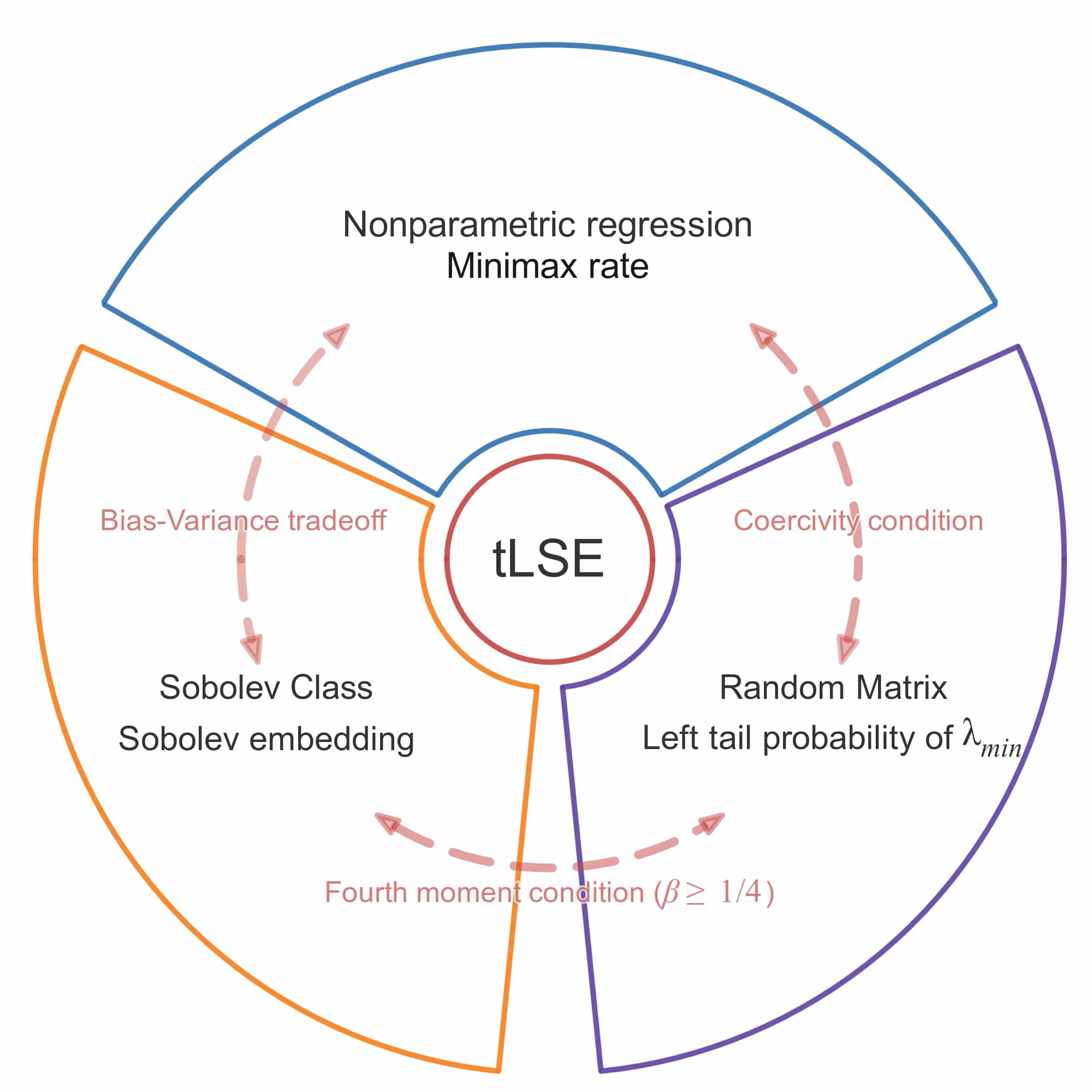
Figure 1: The tLSE method connects the minimax rate with random matrix and Sobolev embedding.

4 Lower bound minimax rate

This section is dedicated to the lower bound minimax rate by the Fano-Tsybakov method [Tsy08, Chapter 2]. The lower rate matches the upper rate in Theorem 3.6, confirming the optimality of the rate.

Recall that $\mathcal{C}(\beta,L)$ is the Hölder continuous class defined in (2.9), $\rho$ is the exploration measure in Definition 2.3, and $\mathbb{E}_{\phi_{*}}$ is the expectation with respect to the dataset $\{(X^{m},Y^{m})\}_{m=1}^{M}$ generated from model (1.1) with $\phi_{*}$. We have our main result on the minimax lower bound. Because $\mathcal{C}(\beta,L)\subseteq W(\beta,L)$ in general, we only need to consider the hypothesis space to be $C(\beta,L)$ for the lower bound.

Theorem 4.1 (Lower bound minimax rate)

Under Assumption 2.1 and Assumption $(\mathrm{B2})$, if $\beta>0$, then there exists a constant $c_{\textup{Lower}}>0$ independent of $M$ such that

$$\liminf_{M\to\infty}\inf_{\widehat{\phi}_{M}}\sup_{\phi_{*}\in\mathcal{C}(\beta,L)}\mathbb{E}_{\phi_{*}}[M^{\frac{2\beta}{2\beta+1}}\|\widehat{\phi}_{M}-\phi_{*}\|_{L^{2}_{\rho}}^{2}]\geq c_{\textup{Lower}}$$ (4.1)

where $\inf_{\widehat{\phi}_{M}}$ is the infimum over all estimators. Here, $c_{\textup{Lower}}=c_{0}c_{\beta,N}$ with $c_{0}$ independent of $M,N$ and $c_{\beta,N}=N^{-\frac{2\beta}{2\beta+1}}$.

Remark 4.2 (Rate in $N$)

The lower bound in (4.1) suggests that $N^{-\frac{2\beta}{2\beta+1}}$ is a lower bound rate in $N$. In other words, the number of particles plays a similar role as the sample size in the lower bound rate. The rate $N^{-\frac{2\beta}{2\beta+1}}$ is the slowest among decay rates $\{N^{-\gamma}\}$ with $\gamma\geq\frac{2\beta}{2\beta+1}$ that can ensure Eq.(4.1).

We follow the general scheme in [Tsy08, Chapter 2 and Theorem 2.11]. This scheme reduces the infimum over all estimators and the supremum over all functions to the bound of the probability of testing error of a finite hypotheses test. We summarize it in three steps, as follows.

1. Reduce (4.1) to bounds in probability by Markov inequality and to a finite number of hypotheses $\Theta=\{\phi_{0,M},\cdots,\phi_{K,M}\}\subseteq\mathcal{C}(\beta,L)$. We set $\phi_{0,M}\equiv 0$ so that $\mathbb{P}_{k}\ll\mathbb{P}_{0}$, where $\mathbb{P}_{k}$ denotes the measure of the model with $\phi_{k,M}$.

2. Transform to bounds in the average probability of the test error of $2s$-separated hypotheses. The key idea in the transformation is a minimum distance test $\kappa_{\text{test}}=\operatorname*{arg\,min}_{1\leq k\leq K}d(\widehat{\phi}_{M},\phi_{k,M})$ [Tsy08, (2.8)].

3. Bound the average probability of the test error from below by the Kullback-Leibler divergence of the hypotheses.

Our main innovation, which is also the major difficulty, is the construction of the hypotheses $\{\phi_{0,M},\phi_{1,M},\cdots,\phi_{K,M}\}\subseteq\mathcal{C}(\beta,L)$ satisfying two conditions: (i) they are 2s-separated in $L^{2}_{\rho}$, and (i) their average Kullback-Leibler divergence $\textup{KL}(\mathbb{P}_{k},\mathbb{P}_{0})$ has a logarithmic growth in $K$. These two conditions are used in the next lemma to prove Step 3. This lemma follows from a combination of a lower bound based on multiple hypotheses, Fano’s lemma, and its corollary, which are in [Tsy08, Theorem 2.6, Lemma 2.10, and Corollary 2.6] respectively, and we omit its proof.

Lemma 4.3 (Lower bound for hypothesis test error )

Let $\Theta=\{\theta_{k}\}_{k=0}^{K}$ with $K\geq 2$ be a set of $2s$-seperated hypotheses, i.e., $d(\theta_{k},\theta_{k^{\prime}})\geq 2s>0$ for all $0\leq k<k^{\prime}\leq K$, for a given metric $d$ on $\Theta$. Denote $\mathbb{P}_{k}=\mathbb{P}_{\theta_{k}}$ and suppose they satisfy $\mathbb{P}_{k}\ll\mathbb{P}_{0}$ for each $k\geq 1$ and

$$\frac{1}{K+1}\sum_{k=1}^{K}\textup{KL}(\mathbb{P}_{k},\mathbb{P}_{0})\leq\alpha\log(K)\,,\quad\text{with }0<\alpha<1/8\,.$$ (4.2)

Then, the average probability of the hypothesis testing error has a lower bound:

$$\ \bar{p}_{e,M}:=\inf_{\kappa_{\text{test}}}\frac{1}{K+1}\sum_{k=0}^{K}\mathbb{P}_{k}\big{(}\kappa_{\text{test}}\neq k\big{)}\geq\frac{\log(K+1)-\log(2)}{\log(K)}-\alpha\,,$$ (4.3)

where $\inf_{\kappa_{\text{test}}}$ denotes the infimum over all tests.

The next lemma constructs the hypothesis functions $\{\phi_{0,M},\phi_{1,M},\cdots,\phi_{K,M}\}$. Its proof is deferred to Section A.4.

Lemma 4.4

For each data set $\{(X^{m},Y^{m})\}_{m=1}^{M}$, there exists a set of hypothesis functions $\{\phi_{0,M}\equiv 0,\phi_{1,M},\cdots,\phi_{K,M}\}$ and positive constants $\{C_{0},C_{1}\}$ independent of $M$and $N$, where

$$K\geq 2^{\bar{K}/8},\quad\text{ with }\bar{K}=\lceil c_{0,N}M^{\frac{1}{2\beta+1}}\rceil,\quad c_{0,N}=C_{0}N^{\frac{1}{2\beta+1}},$$ (4.4)

such that the following conditions hold:

1. Hölder continuity: $\phi_{k,M}\in\mathcal{C}(\beta,L)$ (defined in (2.9)) for each $k=1,\cdots,K$;

2. $2s_{N,M}$-separated: $\|\phi_{k,M}-\phi_{k^{\prime},M}\|_{L^{2}_{\rho}}\geq 2s_{N,M}$ with $s_{N,M}=C_{1}c_{0,N}^{-\beta}M^{-\frac{\beta}{2\beta+1}}$;

3. Kullback-Leibler divergence estimate: $\frac{1}{K}\sum_{k=1}^{K}\textup{KL}(\bar{\mathbb{P}}_{k},\bar{\mathbb{P}}_{0})\leq\alpha\log(K)$ with ${\alpha<1/8}$, where $\bar{\mathbb{P}}_{k}(\cdot)={\mathbb{P}}_{\phi_{k,M}}(\cdot\mid X^{1},\ldots,X^{M})$.

Remark 4.5 (The exponent in $N$)

The exponent for $N$ in $c_{0,N}=C_{0}N^{\frac{1}{2\beta+1}}$ in (4.4) is the smallest possible. That is, when one replaces the the constant $c_{0,N}=C_{0}N^{\frac{1}{2\beta+1}}$ in by $c_{0,N}=C_{0}N^{\gamma}$, the exponent $\gamma$ must satisfy $\gamma\geq\frac{1}{2\beta+1}$. Such a constraint arises when we aim for $\alpha<\frac{1}{8}$ in (A.25) for all $N$.

Proof of Theorem 4.1. The proof consists of three steps. We will denote

$$C_{N}=C_{1}c_{0,N}^{-\beta}$$ (4.5)

so that $s_{N,M}$ in Condition $(\mathrm{C2})$ can be writen as $s_{N,M}=C_{N}M^{-\frac{\beta}{2\beta+1}}$.

Step 1: Reduction to bounds in probability for a finite number of hypothesis functions. Recall that the Markov inequality $\mathbb{E}[|Z|^{2}]\geq c^{2}\mathbb{P}{[|Z|>c]}$ holds for any $c\in\mathbb{R}$ and square-integrable random variable $Z$, and the equalities $\mathbb{P}(A)=\mathbb{E}[\mathbf{1}_{A}]=\mathbb{E}[\mathbb{E}[\mathbf{1}_{A}\mid Z]]=\mathbb{E}[\mathbb{P}(A|Z)]$ hold for any measurable set $A$. Then, we can reduce (4.1) to bounds in probability by

$$\sup_{\phi_{*}\in\mathcal{C}(\beta,L)} \mathbb{E}_{\phi_{*}}[M^{\frac{2\beta}{2\beta+1}}\|\widehat{\phi}_{M}-\phi_{*}\|_{L^{2}_{\rho}}^{2}]\geq\max_{\phi\in\{\phi_{0,M},\cdots,\phi_{K,M}\}}\mathbb{E}_{\phi_{*}}[M^{\frac{2\beta}{2\beta+1}}\|\widehat{\phi}_{M}-\phi_{*}\|_{L^{2}_{\rho}}^{2}]$$

$$\geq C_{N}^{2}\max_{\phi\in\{\phi_{0,M},\cdots,\phi_{K,M}\}}\mathbb{P}_{\phi}\bigg{(}\|\widehat{\phi}_{M}-\phi_{*}\|_{L^{2}_{\rho}}\geq s_{N,M}\bigg{)}$$

$$\geq C_{N}^{2}\frac{1}{K+1}\sum_{k=0}^{K}\mathbb{E}_{X^{1},\cdots,X^{M}}\Big{[}\mathbb{P}_{k}\big{(}\|\widehat{\phi}_{M}-{\phi_{k,M}}\|_{L^{2}_{\rho}}\geq s_{N,M}|X^{1},\cdots,X^{M}\big{)}\Big{]}$$

$$=C_{N}^{2}\mathbb{E}_{X^{1},\cdots,X^{M}}\bigg{[}\frac{1}{K+1}\sum_{k=0}^{K}\mathbb{P}_{k}\big{(}\|\widehat{\phi}_{M}-{\phi_{k,M}}\|_{L^{2}_{\rho}}\geq s_{N,M}|X^{1},\cdots,X^{M}\big{)}\bigg{]}\,.$$ (4.6)

We remark that $\{X^{1},\cdots,X^{M}\}$ inside the expectation are fixed and can be treated as deterministic values in the conditional probability.

Step 2. Transform to bounds in the average probability of testing error of the $2s_{N,M}$-separated hypotheses. Define $\kappa_{\text{test}}:\Omega\to\{0,1,\ldots,M\}$ the minimum distance test

$$\kappa_{\text{test}}=\operatorname*{arg\,min}_{0\leq k\leq K}\|\widehat{\phi}_{M}-\phi_{k,M}\|_{L^{2}_{\rho}}.$$

Then, if $\kappa_{\rm{test}}\neq k$, we have $\|\widehat{\phi}_{M}-\phi_{\kappa_{\text{test}},M}\|_{L^{2}_{\rho}}\leq\|\widehat{\phi}_{M}-\phi_{k,M}\|_{L^{2}_{\rho}}$. Together with Property $(\mathrm{C2})$ in Lemma 4.4 (i.e., the functions in $\Theta$ are $2s_{N,M}$-separated) and the triangle inequality, we obtain

$$2s_{N,M}\leq\|{\phi_{k,M}}-\phi_{\kappa_{\text{test}},M}\|\leq\|\widehat{\phi}_{M}-\phi_{\kappa_{\text{test}},M}\|_{L^{2}_{\rho}}+\|\widehat{\phi}_{M}-\phi_{k,M}\|_{L^{2}_{\rho}}\leq 2\|\widehat{\phi}_{M}-\phi_{k,M}\|_{L^{2}_{\rho}}.$$ (4.7)

That is, $\kappa_{\rm{test}}\neq k$ implies $\|\widehat{\phi}_{M}-{\phi_{k,M}}\|_{L^{2}_{\rho}}\geq s_{N,M}$, and hence, $\mathbb{P}_{k}(\|\widehat{\phi}_{M}-{\phi_{k,M}}\|_{L^{2}_{\rho}}\geq s_{N,M}\mid X^{1},\cdots,X^{M})\geq\mathbb{P}(\kappa_{\rm{test}}\neq k\mid X^{1},\cdots,X^{M})$. Consequently, we have

$$\frac{1}{K+1}\sum_{k=0}^{K}\mathbb{P}_{k}\big{(}\|\widehat{\phi}_{M}-{\phi_{k,M}}\|_{L^{2}_{\rho}}\geq s_{N,M}|X^{1},\cdots,X^{M}\big{)}$$

$$\geq \inf_{\kappa_{\text{test}}}\frac{1}{K+1}\sum_{k=0}^{K}\mathbb{P}_{k}\big{(}\kappa_{\text{test}}\neq k|X^{1},\cdots,X^{M}\big{)}=\inf_{\kappa_{\text{test}}}\frac{1}{K+1}\sum_{k=0}^{K}\bar{\mathbb{P}}_{k}\big{(}\kappa_{\text{test}}\neq k\big{)}=:\bar{p}_{e,M},$$ (4.8)

where $\bar{\mathbb{P}}_{k}(\cdot)={\mathbb{P}}_{\phi_{k,M}}(\cdot\mid X^{1},\ldots,X^{M})$. We call $\bar{p}_{e,M}$ the average probability of testing error.

Step 3: Bound $\bar{p}_{e,M}$ from below. Conditional on each data $\{X^{m}\}_{m=1}^{M}$, the Kullback divergence estimate $(\mathrm{C3})$ holds with $0<\alpha<1/8$, and hence by Lemma 4.3 and the fact that $K=2^{\lceil c_{0,N}M^{\frac{1}{2\beta+1}}\rceil}$ in (4.4) increases exponentially in $M$, we have

$$\bar{p}_{e,M}\geq\frac{\log(K+1)-\log(2)}{\log(K)}-\alpha\geq\frac{1}{2}$$

if $M$ is large. Note that the above lower bound of $\bar{p}_{e,M}$ is independent of the dataset $\{X^{m}\}_{m=1}^{M}$. Together with (4.6) in Step 1 and (4) in Step 2, we obtain with $c_{0}=\frac{1}{2}[C_{1}C_{0}^{-\beta}]^{2}$

$$\sup_{\phi_{*}\in\mathcal{C}(\beta,L)}\mathbb{E}_{\phi_{*}}[\|\widehat{\phi}_{M}-\phi_{*}\|_{L^{2}_{\rho}}^{2}]\geq\frac{C_{N}^{2}}{2}M^{-\frac{2\beta}{2\beta+1}}=c_{0}(NM)^{-\frac{2\beta}{2\beta+1}}$$

for any estimator. Hence, the lower bound (4.1) follows.   

Appendix A Technical results and proofs

A.1 Example: $X$ with uniform distribution

This section explicitly computes the exploration measure $\rho$ in Definition 2.3 and the normal operator ${\bar{\mathcal{L}}}=\frac{(N-1)(N-2)}{N^{2}}\mathcal{L}_{G}+\frac{N-1}{N^{2}}I$ in Definition 2.5. We consider the example with $X$ having i.i.d. components uniformly distributed on $[0,1]$. We will show that the operator $\mathcal{L}_{G}$ is compact and the coercivity constant of ${\bar{\mathcal{L}}}$ is exactly $c_{{\bar{\mathcal{L}}}}=\frac{N-1}{N^{2}}$.

Recall the exploration measure $\rho$ defined in Definition 2.3:

$$\rho(A) =\frac{1}{N(N-1)}\sum_{j\neq i}\mathbb{P}{(|X_{i}-X_{j}|\in A)}=\mathbb{P}{(|X_{1}-X_{2}|\in A)}$$

by exchangeability of $X_{1}$, $X_{2}$ and $X_{3}$. Then, it is easy to see that $\rho$ has a density

$$\rho^{\prime}(r)=(2-2r)\mathbf{1}_{\{0\leq r\leq 1\}}\,.$$ (A.1)

Proposition A.1

Let $X=(X_{1},X_{2},X_{3})$ with $X_{i}\overset{iid}{\sim}U([0,1])$. Then, the operator ${\mathcal{L}_{\overline{G}}}$ defined in (2.4) is a compact integral operator with integral kernel

$$G(r,s) =\frac{\widetilde{G}(r,s)}{\rho^{\prime}(r)\rho^{\prime}(s)}\,,\textup{ with }\widetilde{G}(r,s)=[2-(|r-s|+|r+s|)]-[2-2|r+s|]\mathbf{1}_{\{r+s\leq 1\}}\,.$$ (A.2)

Consequently, the smallest eigenvalue of the normal operator ${\bar{\mathcal{L}}}=\frac{(N-1)(N-2)}{N^{2}}\mathcal{L}_{G}+\frac{N-1}{N^{2}}I$ is $c_{{\bar{\mathcal{L}}}}=\frac{N-1}{N^{2}}$.

Proof. Let us recall the notations $r_{ij}=|X_{i}-X_{j}|$ and $\textbf{r}_{ij}=\frac{X_{i}-X_{j}}{r_{ij}}$ in (2.3). We write $\Phi(X_{i}-X_{j})=\phi(r_{ij})\textbf{r}_{ij}$ and $\Psi(X_{i}-X_{j})=\psi(r_{ij})\textbf{r}_{ij}$ and then have

$$\langle{\mathcal{L}_{G}\phi,\psi}\rangle_{L^{2}_{\rho}} =\mathbb{E}[\phi(r_{12})\textbf{r}_{12}\psi(r_{13})\textbf{r}_{13}]$$

$$=\mathbb{E}[\Phi(X_{1}-X_{2})\Psi(X_{1}-X_{3})]$$

$$=\int_{[0,1]^{3}}\Phi(x_{1}-x_{2})\Psi(x_{1}-x_{3})\prod_{i=1}^{3}dx_{i}\,.$$ (A.3)

We introduce a change of variables:

$$[left=\empheqlbrace\,]x =x_{1}-x_{2}\,;$$

$$y =x_{1}-x_{3}\,;$$

$$z =x_{2}+x_{3}\,;$$

which is equivalent to

$$[left=\empheqlbrace\,]x_{1} =\frac{1}{2}(x+y+z)\,;$$

$$x_{2} =\frac{1}{2}(-x+y+z)\,;$$

$$x_{3} =\frac{1}{2}(x-y+z)\,.$$

Thus, (A.3) becomes

$$\int_{[0,1]^{3}}\Phi(x_{1}-x_{2})\Psi(x_{1}-x_{3})\prod_{i=1}^{3}dx_{i}=\frac{1}{2}\int_{D}\Phi(x)\Psi(y)dxdydz,$$

where the cube $[0,1]^{3}$ is transformed to a region $D$ under the change of variables:

$$D=\bigcup_{j=1}^{4}D_{j}=\bigcup_{j=1}^{4}\left\{(x,y,z):(x,y)\in B_{j}\right\}$$

and the projected disjoint regions $\{B_{j}\}_{j=1}^{4}$ on $(x,y)$-plane are defined as follows

$$B_{1}=\{(x,y):x\in[0,1],y\in[0,1]\}\,, \quad B_{2}=\{(x,y):x\in[0,1],-1+x\leq y\leq 0\}\,,$$

$$B_{3}=\{(x,y):x\in[-1,0],y\in[-1,0]\}\,, \quad B_{4}=\{(x,y):x\in[-1,0],0\leq y\leq 1+x\}\,.$$

Let us consider the decomposition

$$B_{1}=B_{11}\cup B_{12}:=\{(x,y)\in[0,1]^{2}:x>y\}\bigcup\{(x,y)\in[0,1]^{2}:x\leq y\}\,.$$

Thus, let $D_{1}=D_{11}\cup D_{12}$, where the projection of $D_{11}$ to $(x,y)$-plane corresponds to $B_{11}$ and the projection of $D_{12}$ to $(x,y)$-plane corresponds to $B_{12}$. Thus, we have

$$\int_{D_{1}}\Phi(x)\Psi(y)dxdydz =\int_{B_{11}}\int_{x-y}^{2-(x+y)}dz\cdot\Phi(x)\Psi(y)dxdy$$

$$+\int_{B_{12}}\int_{y-x}^{2-(x+y)}dz\cdot\Phi(x)\Psi(y)dxdy$$

$$=\int_{[0,1]^{2}}\Phi(x)\Psi(y)\cdot 2[(1-x)\mathbf{1}_{\{x>y\}}+(1-y)\mathbf{1}_{\{x\leq y\}}]dxdy\,.$$

Note that $\Phi(x)=\phi(x)\frac{x}{|x|}=\phi(x)$ and $\Psi(y)=\psi(y)\frac{y}{|y|}=\psi(y)$ on $\{(x,y)\in[0,1]\times[0,1]\}$. So, with the change of variables $r=x$ and $s=y$ we have

$$\int_{D_{1}}\Phi(x)\Psi(y)dxdydz =\int_{[0,1]^{2}}\phi(r)\psi(s)\cdot 2[1-r\mathbf{1}_{\{r>s\}}-s\mathbf{1}_{\{r\leq s\}}]drds$$

$$=\int_{[0,1]^{2}}\phi(r)\psi(s)\frac{[2-(|r-s|+|r+s|)]}{\rho^{\prime}(r)\rho^{\prime}(s)}\rho(dr)\rho(ds),$$

where $\rho^{\prime}(r)=(2-2r)\mathbf{1}_{\{0\leq r\leq 1\}}$. On $D_{3}$, we get the same formula similarly. On the other hand, $D_{2}$ is a region with the projected domain on $(x,y)$-plane corresponds to $B_{2}$. Then, we get

$$\int_{D_{2}}\Phi(x)\Psi(y)dxdydz =\int_{B_{2}}\int_{x-y}^{2+(y-x)}dz\cdot\Phi(x)\Psi(y)dxdy$$

$$=\int_{0}^{1}\int_{-1}^{0}\Phi(x)\Psi(y)\cdot 2(1+y-x)\mathbf{1}_{\{-1\leq y-x\}}dydx$$

$$=-\int_{[0,1]^{2}}\phi(r)\psi(s)\frac{[2-2|r+s|]}{\rho^{\prime}(r)\rho^{\prime}(s)}\mathbf{1}_{\{r+s\leq 1\}}\rho(dr)\rho(ds)\,.$$

On $D_{4}$, we get the same formula similarly.

In conclusion, we get

$$\mathbb{E}[\Phi(X_{1}-X_{2})\Psi(X_{1}-X_{3})] =\int_{[0,1]^{3}}\Phi(x_{1}-x_{2})\Psi(x_{1}-x_{3})\prod_{i=1}^{3}dx_{i}=\frac{1}{2}\int_{D}\Phi(x)\Psi(y)dxdydz$$

$$=\int_{[0,1]^{2}}\phi(r)\psi(s)\frac{[2-(|r-s|+|r+s|)]}{\rho^{\prime}(r)\rho^{\prime}(s)}\rho(dr)\rho(ds)$$

$$\qquad-\int_{[0,1]^{2}}\phi(r)\psi(s)\frac{[2-2|r+s|]}{\rho^{\prime}(r)\rho^{\prime}(s)}\mathbf{1}_{\{r+s\leq 1\}}\rho(dr)\rho(ds)$$

$$=\int_{[0,1]^{2}}\phi(r)\psi(s)G(r,s)\rho(dr)\rho(ds)$$

with $G$ defined in (A.2).

Now, we show $G(r,s)\in L^{2}(\rho)$. This is

$$\int_{[0,1]\times[0,1]}|G(r,s)|^{2}\rho(dr)\rho(ds)= \int_{[0,1]\times[0,1]}\frac{|\widetilde{G}(r,s)|^{2}}{4(1-r)(1-s)}drds$$

$$= 2\int_{0\leq r<s\leq 1}\frac{|[1-s]-[1-|r+s|]\mathbf{1}_{\{r+s\leq 1\}}|^{2}}{(1-r)(1-s)}drds$$

$$\leq 2\int_{0\leq r<s\leq 1}\frac{(1-s)}{(1-r)}drds=2\int_{0\leq s<r\leq 1}\frac{s}{r}drds$$

$$= \int_{0\leq r\leq 1}rdr=\frac{1}{2}\,.$$

So, we conclude that $\mathcal{L}_{G}$ is a Hilbert-Schmidt integral operator and therefore compact. Consequently, the smallest eigenvalue of the normal operator ${\bar{\mathcal{L}}}$ is $c_{{\bar{\mathcal{L}}}}=\frac{N-1}{N^{2}}$.   

A.2 Proofs for the upper bound minimax rate

This section presents technical proofs in Section 3.2. First, we recall a concentration inequality for random matrix and the Weyls’ inequality, which can be found in [Ver18, T⁺15]. They are used in the proof of the first left tail probability in Lemma 3.11.

Theorem A.2 (Matrix Bernstein’s inequality)

Let $\{X_{i}\}_{i=1}^{M}\subset\mathbb{R}^{n\times n}$ be independent mean zero symmetric random matrices such that $\|X_{i}\|_{op}\leq K$ almost surely for all $i$. Then, for every $t\geq 0$, we have

$$\mathbb{P}\left(\Big{\|}\sum_{i=1}^{M}X_{i}\Big{\|}_{\textup{op}}\geq t\right)\leq 2n\exp\left(-\frac{t^{2}/2}{\sigma^{2}+Kt/3}\right),$$

where $\sigma^{2}=\|\sum_{i=1}^{M}\mathbb{E}[X_{i}^{2}]\|_{\textup{op}}$.

Theorem A.3 (Weyl’s inequality)

For any symmetric matrices $S$ and $T$ with the same dimensions, we have

$$\max_{i}|\lambda_{i}(S)-\lambda_{i}(T)|\leq\|S-T\|_{\textup{op}},$$

where $\lambda_{i}(S)$ is the i-th eigenvalue of $S$ in descending order.

Proof of Lemma 3.10. We prove these bounds by applying the fourth-moment bounds for empirical mean in Lemma A.4. To do so, we only need to show that both $\widebar{\mathbf{A}}_{n}^{M}\bm{\theta}^{*}_{n}-\widebar{\mathbf{A}}_{n}^{\infty}\bm{\theta}^{*}_{n}$ and $\widebar{\mathbf{b}}_{n}^{M}-\widebar{\mathbf{b}}_{n}^{\infty}$ are centered empirical means of two random vectors, each of which random vector has bounded fourth-moment.

We start from $\widebar{\mathbf{A}}_{n}^{M}\bm{\theta}^{*}_{n}-\widebar{\mathbf{A}}_{n}^{\infty}\bm{\theta}^{*}_{n}$. Let $\phi_{n}^{*}=\sum_{k=1}^{n}\theta_{k}^{*}\psi_{k}$. Since $R_{\phi}[X]$ is linear in $\phi$, we have $R_{\phi_{n}^{*}}[X]=\sum_{k=1}^{n}\theta_{k}^{*}R_{\psi_{k}}[X]$ for any $X$. Define an $\mathbb{R}^{n}$-valued random vector $Z_{A}$ to be

$$Z_{A}(l)=\frac{1}{N}\langle{R_{\psi_{l}}[X],R_{\phi_{n}^{*}}[X]}\rangle_{\mathbb{R}^{Nd}},\quad 1\leq l\leq n.$$ (A.4)

Then, we can write the $\mathbb{R}^{n}$-valued random variable $\widebar{\mathbf{A}}_{n}^{M}\bm{\theta}^{*}_{n}$ as

$$[\widebar{\mathbf{A}}_{n}^{M}]\bm{\theta}^{*}_{n}(l) =\sum_{k=1}^{n}\frac{1}{MN}\sum_{m=1}^{M}\langle{R_{\psi_{l}}[X^{m}],R_{\psi_{k}}[X^{m}]}\rangle_{\mathbb{R}^{Nd}}\theta_{k}^{*}$$

$$=\frac{1}{M}\sum_{m=1}^{M}\frac{1}{N}\langle{R_{\psi_{l}}[X^{m}],R_{\phi_{n}^{*}}[X^{m}]}\rangle_{\mathbb{R}^{Nd}}=\frac{1}{M}\sum_{m=1}^{M}Z_{A}^{m}(l),$$

where $Z_{A}^{m}(l)=\frac{1}{N}\langle{R_{\psi_{l}}[X^{m}],R_{\phi_{n}^{*}}[X^{m}]}\rangle_{\mathbb{R}^{Nd}}$ is a sample of $Z_{A}(l)$ for each $m$. Also, $\widebar{\mathbf{A}}_{n}^{\infty}\bm{\theta}^{*}_{n}(l)=\mathbb{E}[Z_{A}(l)]$ for each $l$ by the definition of $\widebar{\mathbf{A}}_{n}^{\infty}$. Meanwhile, note that by definition of $Z_{A}$, the boundedness of the basis functions in Assumption 2.12, and the definition of the operator $R_{\phi}[X]$, we have

$$|Z_{A}(l)| =\Big{|}\frac{1}{N}\sum_{i=1}^{N}\frac{1}{N^{2}}\sum_{j\neq i}\sum_{j^{\prime}\neq i}\psi_{l}(r_{ij})\phi_{n}^{*}(r_{ij^{\prime}})\langle{\textbf{r}_{ij},\textbf{r}_{ij^{\prime}}}\rangle_{\mathbb{R}^{d}}\Big{|}$$

$$\leq\sup_{k\geq 1}\|\psi_{k}\|_{\infty}^{2}\sup_{k\geq 1}|\theta_{k}^{*}|\leq C_{\max}^{2}\sup_{k\geq 1}|\theta_{k}^{*}|.$$

Thus, we have shown that $\widebar{\mathbf{A}}_{n}^{M}\bm{\theta}^{*}_{n}-\widebar{\mathbf{A}}_{n}^{\infty}\bm{\theta}^{*}_{n}$ is the centered empirical mean of i.i.d. samples of a bounded random vector $Z_{A}$ (hence its fourth-moment). As a result, applying Lemma A.4, we obtain

$$\mathbb{E}\|(\widebar{\mathbf{A}}_{n}^{M}-\widebar{\mathbf{A}}_{n}^{\infty})\bm{\theta}^{*}_{n}\|_{\mathbb{R}^{n}}^{4}\leq\frac{6M-5}{M^{3}}n2^{5}\mathbb{E}|Z_{A}|^{4}\leq\frac{n^{2}}{M^{2}}192C_{\max}^{8}(\sup\nolimits_{k\geq 1}|\theta_{k}^{*}|)^{4}.$$

Taking square root and using the fact that $\sup_{k\geq 1}|\theta_{k}^{*}|^{2}\leq L$ in Lemma 2.16, we obtain (3.14a).

The proof for the bound in (3.14b) is similar. By definition, the normal vector $\widebar{\mathbf{b}}_{n}^{M}=\frac{1}{M}\sum_{m=1}^{M}\mathbf{b}_{n}^{m}$ is the average of $M$ samples $\{\mathbf{b}_{n}^{m}\}_{m=1}^{M}$ of the $\mathbb{R}^{n}$-value random vector $\mathbf{b}_{n}$ with entries

$$\mathbf{b}_{n}(l)=\frac{1}{N}\langle{R_{\psi_{l}}[X],R_{\phi_{*}}[X]+\bm{\eta}}\rangle_{\mathbb{R}^{Nd}},\quad 1\leq l\leq n.$$

To show that $\mathbf{b}_{n}$ has a bounded fourth-moment, we decompose it into a bounded part and an unbounded part, $\mathbf{b}_{n}=\xi+\tilde{\eta}$, where

$$\xi(l)=\frac{1}{N}\langle{R_{\psi_{l}}[X],R_{\phi_{*}}[X]}\rangle_{\mathbb{R}^{Nd}},\quad\widetilde{\eta}(l)=\frac{1}{N}\langle{R_{\psi_{l}}[X],\bm{\eta}}\rangle_{\mathbb{R}^{Nd}}.$$

The random vector $\xi$ is bounded because by the boundedness of the eigen-functions in Assumption 2.12, we have

$$|\xi(l)| \leq\sup_{k\geq 1}\|\psi_{k}\|_{\infty}^{2}\sup_{k\geq 1}|\theta_{k}^{*}|\leq C_{\max}^{2}\sup_{k\geq 1}|\theta_{k}^{*}|.$$

To bound the noise term, we use the Cauchy-Schwarz inequality,

$$\mathbb{E}|\widetilde{\eta}(l)|^{4} =\frac{1}{N^{4}}\mathbb{E}[|\langle{R_{\psi_{l}}[X],\bm{\eta}}\rangle_{\mathbb{R}^{Nd}}|^{4}]\leq\frac{1}{N^{4}}\mathbb{E}[|\|R_{\psi_{l}}[X]\|\|\bm{\eta}\||^{4}]\leq\frac{1}{N^{2}}C_{\max}^{4}C_{\eta},$$

where the first inequality follows from the assumption that the fourth moment of $\bm{\eta}$ is bounded by some constant $C_{\eta}>0$, and the last inequality follows from that $\|R_{\psi_{l}}[X]\|^{2}\leq NC_{\max}^{2}$ for all $X$.

Combining these bounds, we have, for $1\leq l\leq n$,

$$\mathbb{E}|\mathbf{b}_{n}(l)|^{4} \leq\mathbb{E}|\xi(l)+\widetilde{\eta}(l)|^{4}\leq 2^{4}\mathbb{E}\Big{[}|\xi(l)|^{4}+|\widetilde{\eta}(l)|^{4}\Big{]}$$

$$\leq 2^{4}[C_{\max}^{8}\sup_{l\geq 1}|\theta_{l}^{*}|^{4}+\frac{1}{N^{2}}C_{\max}^{4}C_{\eta}]\leq 2^{4}C_{\max}^{4}[C_{\max}^{4}\sup_{l\geq 1}|\theta_{l}^{*}|^{4}+\frac{1}{N^{2}}C_{\eta}].$$

Consequently, applying Lemma A.4 with $Z_{m}(k)=\frac{1}{N}\langle{R_{\psi_{k}}[X^{m}],Y^{m}}\rangle_{\mathbb{R}^{Nd}}$, we obtain

$$\mathbb{E}[\|\widebar{\mathbf{b}}_{n}^{M}-\widebar{\mathbf{b}}_{n}^{\infty}\|_{\mathbb{R}^{n}}^{4}] \leq\frac{n^{2}(6M-5)}{M^{3}}2^{9}C_{\max}^{4}[C_{\max}^{4}\sup_{l\geq 1}|\theta_{l}^{*}|^{4}+\frac{1}{N^{2}}C_{\eta}]\leq C_{b}^{2}\frac{n^{2}}{M^{2}}$$

with $C_{b}=2^{5}\sqrt{3}C_{\max}^{2}(C_{\max}^{4}L^{2}+\frac{1}{N^{2}}C_{\eta})^{1/2}$, using again the fact that $\sup_{k\geq 1}|\theta_{k}^{*}|^{2}\leq L$ in Lemma 2.16.   

The next lemma provides bounds for the fourth moment of the empirical mean of i.i.d. samples. It is of general interest beyond this study. The proof follows from applying the independence between the samples and the direct expansion of the fourth power of the sum.

Lemma A.4 (fourth-moment bounds of empirical mean)

Let $\{Z_{m}\}_{m=1}^{M}$ be i.i.d. samples of the $R^{n}$-valued random variable $Z=(Z(1),\ldots,Z(n))$. Assume that $\sum_{k=1}^{n}\mathbb{E}|Z(k)|^{4}<\infty$. Then,

$$\mathbb{E}\Big{|}\frac{1}{M}\sum_{m=1}^{M}(Z_{m}-\mathbb{E}[Z])\Big{|}^{4}\leq\frac{6n}{M^{2}}\sum_{k=1}^{n}\mathbb{E}|Z(k)-\mathbb{E}[Z(k)]|^{4}\leq\frac{2^{8}n}{M^{2}}\sum_{k=1}^{n}\mathbb{E}|Z(k)|^{4}.$$

Proof. The second inequality follows directly from

$$\mathbb{E}|Z(k)-\mathbb{E}[Z(k)]|^{4}\leq 2^{4}\left(\mathbb{E}|Z(k)|^{4}+\mathbb{E}|\mathbb{E}[Z(k)]|^{4}\right)\leq 2^{5}\mathbb{E}|Z(k)|^{4}$$

for each $1\leq k\leq n$ since $\mathbb{E}|\mathbb{E}[Z(k)]|^{4}\leq\mathbb{E}|Z(k)|^{4}$ by Jensen’s inequality.

To prove the first inequality, it suffices to consider $\mathbb{E}[Z]=0$ and prove

$$\mathbb{E}\bigg{|}\frac{1}{M}\sum_{m=1}^{M}Z_{m}\bigg{|}^{4}\leq\frac{6n}{M^{2}}\sum_{k=1}^{n}\mathbb{E}|Z(k)|^{4}.$$ (A.5)

We first prove the case with $n=1$, then extend it to the case with $n>1$.

Case $n=1$: $Z$ is a 1-dimensional random variable. Note that

$$\Big{|}\sum_{m=1}^{M}Z_{m}\Big{|}^{4} =\sum_{m_{1},\cdots,m_{4}=1}^{M}\prod_{i=1}^{4}Z_{m_{i}}$$

$$=\sum_{m=1}^{M}Z_{m}^{4}+4\sum_{\begin{subarray}{c}m_{1},m_{2}=1\\ m_{1}\neq m_{2}\end{subarray}}^{M}Z_{m_{1}}Z_{m_{2}}^{3}+6\sum_{\begin{subarray}{c}m_{1},m_{2}=1\\ m_{1}\neq m_{2}\end{subarray}}^{M}Z_{m_{1}}^{2}Z_{m_{2}}^{2}$$

$$+6\sum_{\begin{subarray}{c}m_{1},m_{2},m_{3}=1\\ m_{1}\neq m_{2}\neq m_{3}\end{subarray}}^{M}Z_{m_{1}}^{2}Z_{m_{2}}Z_{m_{3}}+\sum_{\begin{subarray}{c}m_{1},m_{2},m_{3},m_{4}=1\\ m_{1}\neq m_{2}\neq m_{3}\neq m_{4}\end{subarray}}^{M}Z_{m_{1}}Z_{m_{2}}Z_{m_{3}}Z_{m_{4}}\,.$$

Meanwhile, the independence between these mean zero samples implies that $\mathbb{E}[Z_{m_{1}}Z_{m_{2}}^{3}]=0$, $\mathbb{E}[Z_{m_{1}}^{2}Z_{m_{2}}Z_{m_{3}}]=0$, and $\mathbb{E}[Z_{m_{1}}Z_{m_{2}}Z_{m_{3}}Z_{m_{4}}]=0$, for any mutually different indices $1\leq m_{1},m_{2},m_{3},m_{4}\leq M$. Then, the desired inequality in (A.5) with $n=1$ follows from

$$\mathbb{E}\Big{|}\sum_{m=1}^{M}Z_{m}\Big{|}^{4} =\mathbb{E}[\sum_{m=1}^{M}Z_{m}^{4}+6\sum_{\begin{subarray}{c}m_{1},m_{2}=1\\ m_{1}\neq m_{2}\end{subarray}}^{M}Z_{m_{1}}^{2}Z_{m_{2}}^{2}]$$

$$=M\mathbb{E}[|Z|^{4}]+6M(M-1)(\mathbb{E}[|Z^{2}|])^{2}\leq 6M^{2}\mathbb{E}|Z|^{4},$$

where the second equality follows from that $\{Z_{m}\}$ are samples of $Z$, and the last inequality follows from $(\mathbb{E}[|Z^{2}|])^{2}\leq\mathbb{E}|Z|^{4}$ by Jensen’s inequality.

Case $n>1$: $Z$ is a random vector. We prove it by applying the above bound to each component of the vector. Note that

$$\Big{|}\frac{1}{M}\sum_{m=1}^{M}Z_{m}\Big{|}^{4}=\left(\sum_{k=1}^{n}\Big{|}\frac{1}{M}\sum_{m=1}^{M}Z_{m}(k)\Big{|}^{2}\right)^{2}\leq n\sum_{k=1}^{n}\Big{|}\frac{1}{M}\sum_{m=1}^{M}Z_{m}(k)\Big{|}^{4}.$$

Meanwhile, applying the result in Case $n=1$ to each component $\{Z_{m}(k)\}$, we have

$$\mathbb{E}\bigg{|}\frac{1}{M}\sum_{m=1}^{M}Z_{m}(k)\bigg{|}^{4}\leq\frac{6}{M^{2}}\mathbb{E}|Z(k)|^{4},\quad\forall 1\leq k\leq n.$$

Combining the two inequalities, we obtain the inequality (A.5).   

A.3 Proof for the 2nd left tail probability

Here, we include some technical proofs in Section 3.3.

Lemma A.5 (PAC-Bayesian inequality)

Let $\Theta$ be a measurable space, and $\{Z(\theta):\theta\in\Theta\}$ be a real-valued measurable process. Assume that

$$\mathbb{E}[\exp(Z(\theta))]\leq 1\,,\quad\text{for every }\theta\in\Theta\,.$$ (A.6)

Let $\pi$ be a probability distribution on $\theta$. Then,

$$\mathbb{P}\left\{\forall\mu,\int_{\Theta}Z(\theta)\mu(\theta)\leq\textup{KL}(\mu,\pi)+t\right\}\geq 1-e^{-t}\,,$$ (A.7)

where $\mu$ spans all probability measures on $\Theta$, and $\textup{KL}(\mu,\pi)$ is the Kullback-Leibler divergence between $\mu$ and $\pi$:

$$\textup{KL}(\mu,\pi):=\begin{cases}\int_{\Theta}\log\Big{[}\frac{d\mu}{d\pi}\Big{]}d\mu&\text{if }\mu\ll\pi\,;\\ \infty&\text{otherwise}\,.\end{cases}$$

The next lemma, from [Mou22, Section 2.3], controls the approximate term in the application of the PAC-inequality. Here we present an alternative constructive proof.

Lemma A.6

For every $\gamma\in(0,1/2]$, $v\in S^{n-1}$, define

$$\Theta_{v,\gamma}:=\{\theta\in S^{n-1}:\|\theta-v\|\leq\gamma\},\quad\text{ and }\pi_{v,\gamma}(d\theta)=\frac{\bf 1_{\Theta_{v,\gamma}}(\theta)}{\pi(\Theta_{v,\gamma})}\pi(d\theta),$$ (A.8)

where $\pi$ is a uniform measure on the sphere. That is, $\Theta_{v,\gamma}$ is a “spherical cap” or “contact lens” in $n$-th dimension space, and $\pi_{v,\gamma}$ is a uniform surface measure on the spherical cap. Then,

$$F_{v,\gamma}(\Sigma):=\int_{\Theta}\langle{\Sigma\theta,\theta}\rangle\pi_{v,\gamma}(d\theta)=[1-g(\gamma)]\langle{\Sigma v,v}\rangle+g(\gamma)\frac{\textup{Tr}(\Sigma)}{n},$$ (A.9)

for any symmetric matrix $\Sigma$, where

$$g(\gamma)=\frac{n}{n-1}\int_{\Theta}[1-\langle{\theta,v}\rangle^{2}]\pi_{v,\gamma}(d\theta)\in\bigg{[}0,\frac{n\gamma^{2}}{(n-1)}\bigg{]}\,.$$ (A.10)

Proof of Lemma A.6. Note that

$$F_{v,\gamma}(\Sigma) :=\int_{\Theta}\langle{\Sigma\theta,\theta}\rangle\pi_{v,\gamma}(d\theta)=\int_{\Theta}\textup{Tr}[\theta^{\top}\Sigma\theta]\pi_{v,\gamma}(d\theta)$$

$$=\textup{Tr}[\Sigma A_{v,\gamma}]:=\textup{Tr}\left[\Sigma\int_{\Theta}\theta\theta^{\top}\pi_{v,\gamma}(d\theta)\right]\,.$$

To conclude (A.9), we proceed to show that

$$A_{v,\gamma}=[1-g(\gamma)]vv^{\top}+g(\gamma)\frac{I_{n}}{n}\,.$$ (A.11)

By isometric invariance, we set without loss of generality

$$v=e_{1}=(1,0,\cdots,0)\in\mathbb{R}^{n}\,.$$

So we get a $\mathbb{R}^{n}$-“spherical cap” $\Theta_{\gamma}=\Theta(e_{1},\gamma)$ centered at $v=e_{1}$. The notations $A_{e_{1},\gamma}$ and $\pi_{e_{1},\gamma}(d\theta)$ are abbreviated as $A_{\gamma}$ and $\pi_{\gamma}(d\theta)$. Thus, for $\theta=(\theta_{1},\theta_{2},\cdots,\theta_{n})\in\Theta_{\gamma}\subseteq S^{n-1}$ we have

$$A_{\gamma} =\int_{\Theta_{\gamma}}\theta\theta^{\top}\pi_{\gamma}(d\theta)=\int_{\Theta_{\gamma}}\begin{bmatrix}\theta_{1}^{2}&\theta_{1}\theta_{2}&\cdots&\theta_{1}\theta_{n}\\ \theta_{2}\theta_{1}&\theta_{2}^{2}&\cdots&\theta_{2}\theta_{n}\\ \vdots&\vdots&\vdots&\vdots\\ \theta_{n}\theta_{1}&\theta_{n}\theta_{2}&\cdots&\theta_{n}^{2}\end{bmatrix}\pi_{\gamma}(d\theta)$$

$$=\text{diag}\left[\int_{\Theta_{\gamma}}\theta_{1}^{2}\pi_{\gamma}(d\theta),\int_{\Theta_{\gamma}}\theta_{2}^{2}\pi_{\gamma}(d\theta),\cdots,\int_{\Theta_{\gamma}}\theta_{2}^{2}\pi_{\gamma}(d\theta)\right]$$

since $\int_{\Theta_{\gamma}}\theta_{2}^{2}\pi_{\gamma}(d\theta)=\cdots=\int_{\Theta_{\gamma}}\theta_{n}^{2}\pi_{\gamma}(d\theta)$ and $\int_{\Theta_{\gamma}}\theta_{i}\theta_{j}\pi_{\gamma}(d\theta)=0$ if $i\neq j$. Moreover, it is readily seen that

$$1=\int_{\Theta_{\gamma}}\|\theta\|^{2}\pi_{\gamma}(d\theta)=\int_{\Theta_{\gamma}}[\theta_{1}^{2}+\theta_{2}^{2}+\cdots+\theta_{n}^{2}]\pi_{\gamma}(d\theta)=\int_{\Theta_{\gamma}}\theta_{1}^{2}\pi_{\gamma}(d\theta)+(n-1)\int_{\Theta_{\gamma}}\theta_{2}^{2}\pi_{\gamma}(d\theta)\,,$$

and consequently

$$\int_{\Theta_{\gamma}}\theta_{2}^{2}\pi_{\gamma}(d\theta)=\cdots=\int_{\Theta_{\gamma}}\theta_{n}^{2}\pi_{\gamma}(d\theta)=\frac{1}{n-1}\left[1-\int_{\Theta_{\gamma}}\theta_{1}^{2}\pi_{\gamma}(d\theta)\right]=\frac{g(\gamma)}{n}\,.$$

Hence, we have

$$A_{\gamma}=\text{diag}\left[\int_{\Theta_{\gamma}}\theta_{1}^{2}\pi_{\gamma}(d\theta),\frac{g(\gamma)}{n},\cdots,\frac{g(\gamma)}{n}\right]\,.$$ (A.12)

Noticing that $g(\gamma)=\frac{n}{n-1}\left[1-\int_{\Theta_{\gamma}}\theta_{1}^{2}\pi_{\gamma}(d\theta)\right]$ and $(1-g(\gamma))+\frac{g(\gamma)}{n}=\int_{\Theta_{\gamma}}\theta_{1}^{2}\pi_{\gamma}(d\theta)$, the right-hand side of (A.11) can be written as

$$(1-g(\gamma))vv^{\top}+g(\gamma)\frac{I_{n}}{n}=\text{diag}\left[\int_{\Theta_{\gamma}}\theta_{1}^{2}\pi_{\gamma}(d\theta),\frac{g(\gamma)}{n},\cdots,\frac{g(\gamma)}{n}\right]\,,$$

which matches (A.12).

The bound of $g(\gamma)$ in (A.10) can follow the same argument in [Mou22]. This completes the proof.   

We introduce an inequality in [Oli16, Lemma A.1] to control the generating moment function before the proof of 3.12.

Lemma A.7

Let $X$ be a nonnegative random variable with a finite second moment. Then for all $\lambda\geq 0$

$$\mathbb{E}[e^{-\lambda X}]\leq e^{-\lambda\mathbb{E}[X]+\frac{\lambda^{2}}{2}\mathbb{E}[X^{2}]}\,.$$

Proof. We include the proof for completeness. It is clear that

$$\mathbb{E}[e^{-\lambda X}]\leq 1-\lambda\mathbb{E}[X]+\frac{\lambda^{2}}{2}\mathbb{E}[X^{2}]\leq e^{-\lambda\mathbb{E}[X]+\frac{\lambda^{2}}{2}\mathbb{E}[X^{2}]}$$

by using $1+y\leq e^{y}$ in the second inequality.   

Proof of Lemma 3.12. Step 1: For every $\theta\in S^{n-1}$ and $\lambda>0$, the bound for the moment generating function can be derived by Lemma A.7:

$$\mathbb{E}\left[\exp\left(-\lambda\frac{1}{N}\|R_{\phi_{\theta}}[X^{m}]\|^{2}\right)\right] \leq\exp\left(-\lambda\frac{1}{N}\mathbb{E}[\|R_{\phi_{\theta}}[X^{m}]\|^{2}]+{\frac{\lambda^{2}}{2N^{2}}\mathbb{E}[\|R_{\phi_{\theta}}[X^{m}]\|^{4}]}\right)$$

$$\leq\exp\left(-\lambda c_{\bar{\mathcal{L}}}+{\frac{\lambda^{2}}{2N^{2}}\mathbb{E}[\|R_{\phi_{\theta}}[X^{m}]\|^{4}]}\right)\,.$$

By (2.11) and Jensen’s inequality

$$\mathbb{E}[\|R_{\phi_{\theta}}[X^{m}]\|^{4}] \leq\kappa\cdot\left(\mathbb{E}[\|R_{\phi_{\theta}}[X^{m}]\|^{2}]\right)^{2}\leq\kappa\cdot\left(\mathbb{E}\left[\sum_{i=1}^{N}\left|R_{\phi_{\theta}}[X^{m}]_{i}\right|^{2}\right]\right)^{2}$$

$$=\kappa\cdot\left(\mathbb{E}\left[\sum_{i=1}^{N}\left|\frac{1}{N-1}\sum_{j\neq i}\phi_{\theta}(r^{m}_{ij})\mathbf{r}^{m}_{ij}\right|^{2}\right]\right)^{2}$$

$$\leq\kappa\cdot\left(\sum_{i=1}^{N}\frac{1}{N-1}\sum_{j\neq i}\mathbb{E}\left[\left|\phi_{\theta}(r^{m}_{ij})\right|^{2}\right]\right)^{2}\,.$$

Remember that $\phi_{\theta}(r^{m}_{ij})=\sum_{k=1}^{n}\theta_{k}\psi_{k}(r^{m}_{ij})$, the distribution of random variable $r^{m}_{ij}$ is $\rho$ and $\{\psi_{k}\}$ are ONB in $L^{2}_{\rho}$, then we can proceed to get

$$\frac{1}{N-1}\sum_{j\neq i}\mathbb{E}\left[\left|\phi_{\theta}(r^{m}_{ij})\right|^{2}\right]=\frac{1}{N-1}\sum_{j\neq i}\mathbb{E}\left[\left|\sum_{k=1}^{n}\theta_{k}\psi_{k}(r^{m}_{ij})\right|^{2}\right]=\sum_{k=1}^{n}\theta_{k}^{2}=1\,.$$

Therefore, we have

$${\mathbb{E}[\|R_{\phi_{\theta}}[X^{m}]\|^{4}]\leq\kappa N^{2}\,.}$$ (A.13)

Combing (A.13) and the fact that $\frac{1}{N}\mathbb{E}[\|R_{\phi_{\theta}}[X^{m}]\|^{2}]\geq c_{\bar{\mathcal{L}}}$, we obtain

$$\mathbb{E}\left[\exp\left(-\frac{\lambda}{N}\|R_{\phi_{\theta}}[X^{m}]\|^{2}+\lambda c_{\bar{\mathcal{L}}}-\frac{\lambda^{2}}{2}{\kappa N^{2}}\right)\right]\leq 1,\quad\forall\theta\in S^{n-1},\lambda>0.$$ (A.14)

Thus, by the independence of samples, we obtain

$$\sup_{\theta\in S^{n-1}}\mathbb{E}\left[\exp\left(-\frac{\lambda}{N}\sum_{m=1}^{M}\|R_{\phi_{\theta}}[X^{m}]\|^{2}+\lambda Mc_{\bar{\mathcal{L}}}-\frac{\lambda^{2}}{2}{\kappa MN^{2}}\right)\right]\leq 1,\quad\forall\lambda>0.$$

In other words, the process

$$Z_{\lambda}(\theta):=-\frac{\lambda}{N}\sum_{m=1}^{M}\|R_{\phi_{\theta}}[X^{m}]\|^{2}+\lambda Mc_{\bar{\mathcal{L}}}-\frac{\lambda^{2}}{2}{\kappa MN^{2}}$$

with $\theta\in S^{n-1}$ has a uniformly bounded moment generating function. Then, applying the PAC-Bayes inequality in Lemma A.5 with $\Theta=S^{n-1}$, we obtain

$$\mathbb{P}\left\{\sup_{\mu\in\mathcal{P}}\int_{\Theta}Z_{\lambda}(\theta)\mu(\theta)\leq\textup{KL}(\mu,\pi)+t\right\}\geq 1-e^{-t},\quad\forall t>0,$$ (A.15)

where $\pi,\mu\in\mathcal{P}$ with $\mathcal{P}$ denoting the set of all probability measures on $\Theta$. In the next step, we will select a specific $\pi$ and a subset of $\mathcal{P}$ in (A.15) to obtain a $\lambda$-dependent bound $\mathbb{P}\left\{\lambda_{min}(\mathbf{A}_{n}^{M})<\frac{1}{8}c_{\bar{\mathcal{L}}}\right\}$, and we remove the dependence on $\lambda$ in Step 3.

Step 2: Obtain a lower bound for $\lambda_{min}(\mathbf{A}_{n}^{M})$ through constructing probability measures $\pi$ and $\mu$ in (A.15) to control $\int_{\Theta}Z_{\lambda}(\theta)\mu(d\theta)$. This lower bound depends on $\lambda$, which will be selected in Step 3 to achieve the desired bound in (3.18).

Let $\pi$ be a uniform probability measure on $S^{n-1}$. For each $v\in S^{n-1}$ and $\gamma\in(0,1/2]$, define $\Theta_{v,\gamma}$ and probability measures $\pi_{v,\gamma}$ as in (A.8). Then, the PAC-Bayesian inequality (A.15) with $\mu(d\theta)=\pi_{v,\gamma}(d\theta)$ implies that

$$\mathbb{P}\left\{\sup_{v\in S^{n-1},\gamma\in(0,1/2]}\int_{\Theta}Z_{\lambda}(\theta)\pi_{v,\gamma}(\theta)-\textup{KL}(\pi_{v,\gamma},\pi)\leq t\right\}\geq 1-e^{-t}\,.$$

Meanwhile, note that

$$\frac{1}{M}\int_{\Theta}Z_{\lambda}(\theta)\pi_{v,\gamma}(d\theta) =\bigg{[}-\lambda\int_{\Theta}\langle{\bar{\mathbf{A}}_{n}^{M}\theta,\theta}\rangle\pi_{v,\gamma}(d\theta)+\lambda c_{\bar{\mathcal{L}}}-\frac{\lambda^{2}}{2}{\kappa N^{2}}\bigg{]}$$

$$=:[-\lambda F_{v,\gamma}(\bar{\mathbf{A}}_{n}^{M})+\lambda c_{\bar{\mathcal{L}}}-\frac{\lambda^{2}}{2}{\kappa N^{2}}]\,.$$

Hence, the above inequality implies that, with at least probability $1-e^{-Mu}$,

$$\sup_{v\in S^{n-1},\gamma\in(0,1/2]}\bigg{[}-\lambda F_{v,\gamma}(\bar{\mathbf{A}}_{n}^{M})+\lambda c_{\bar{\mathcal{L}}}-\frac{\lambda^{2}}{2}{\kappa N^{2}}-\frac{1}{M}\textup{KL}(\pi_{v,\gamma},\pi)\bigg{]}\leq\frac{t}{M}=u.$$

$$\Leftrightarrow\quad \inf_{v\in S^{n-1},\gamma\in(0,1/2]}\lambda F_{v,\gamma}(\bar{\mathbf{A}}_{n}^{M})+\frac{1}{M}\textup{KL}(\pi_{v,\gamma},\pi)\geq\lambda c_{\bar{\mathcal{L}}}-\frac{\lambda^{2}}{2}{\kappa N^{2}}-u\,.$$ (A.16)

Follow the conventions in [Mou22], we refer $F_{v,\gamma}(\bar{\mathbf{A}}_{n}^{M})$ to be the approximation term and $\textup{KL}(\pi_{v,\gamma},\pi)$ the entropy term. The controls of these terms follow from the above selection of measure $\pi_{v,\gamma}$ and $\pi$.

The control of approximate term follows from applying Lemma A.6 with $\Sigma=\bar{\mathbf{A}}_{n}^{M}$:

$$F_{v,\gamma}(\bar{\mathbf{A}}_{n}^{M})=[1-g(\gamma)]\langle{\bar{\mathbf{A}}_{n}^{M}v,v}\rangle+g(\gamma)\frac{\textup{Tr}(\Sigma)}{n}$$

with $g(\gamma)$ in (A.10). The control of the entropy term is from Section 2.4 in the supplement of [Mou22]). Specifically, we have for every $v\in S^{n-1}$ and $\gamma>0$,

$$\textup{KL}(\pi_{v,\gamma},\pi) =\int_{\Theta}\log\left(\frac{d\pi_{v,\gamma}}{d\pi}(\theta)\right)\pi_{v,\gamma}(d\theta)=\int_{\Theta}\log\left[\frac{1}{\pi(\Theta_{v,\gamma})}\right]\pi_{v,\gamma}(d\theta)$$

$$=\log\left[\frac{1}{\pi(\Theta_{v,\gamma})}\right]\leq n\log(1+2/\gamma)\,,$$

where the bound for surface area $\pi(\Theta_{v,\gamma})$ is from [Ver18, Lemma 4.2.13].

Plugging these two estimates into (A.16) we obtain with at least probability $1-e^{-Mu}$, for all $v\in S^{n-1},\gamma\in(0,1/2]$,

$$\lambda(1-g(\gamma))\langle{\bar{\mathbf{A}}_{n}^{M}v,v}\rangle-\lambda g(\gamma)\frac{\text{Tr}(\bar{\mathbf{A}}_{n}^{M})}{n}+n\log(1+2/\gamma)\geq\lambda c_{\bar{\mathcal{L}}}-\frac{\lambda^{2}}{2}{\kappa N^{2}}-u,\,$$

which amounts to

$$\langle{\bar{\mathbf{A}}_{n}^{M}v,v}\rangle \geq\frac{1}{\lambda(1-g(\gamma))}\bigg{[}\lambda c_{\bar{\mathcal{L}}}-\frac{\lambda^{2}}{2}{\kappa N^{2}}-\frac{n}{M}\log(1+2/\gamma)-u\bigg{]}-\frac{g(\gamma)}{1-g(\gamma)}\frac{\text{Tr}(\bar{\mathbf{A}}_{n}^{M})}{n}\,.$$ (A.17)

Also, the uniform boundedness of $\{\psi_{k}\}$ in Assumption 2.12 implies:

$$\frac{\text{Tr}(\bar{\mathbf{A}}_{n}^{M})}{n}=\frac{1}{nMN}\sum_{m=1}^{M}\sum_{k=1}^{n}\|R_{\psi_{k}}(X^{m})\|_{\mathbb{R}^{Nd}}^{2}\leq C_{\max}^{2}<\infty.$$

Moreover, when $\gamma\in(0,1/2]$ we have by (A.10)

$$\frac{g(\gamma)}{1-g(\gamma)}\leq\frac{2\gamma^{2}}{1-g(\gamma)}\quad\text{ and }\quad\log(1+2/\gamma)\leq\log\left(\frac{5}{4\gamma^{2}}\right)\,.$$

Letting $c_{\gamma}:=\frac{1}{1-g(\gamma)}$, one can note that $1\leq c_{\gamma}\leq 2$ and $c_{\gamma}\to 1$ as $\gamma\to 0$. Therefore, we have for every $\gamma\in(0,1/2]$ and $u>0$

$$\inf_{v\in S^{n-1}}\langle{\bar{\mathbf{A}}_{n}^{M}v,v}\rangle \geq\frac{c_{\gamma}}{\lambda}\bigg{[}\lambda c_{\bar{\mathcal{L}}}-\frac{\lambda^{2}}{2}{\kappa N^{2}}-\frac{n}{M}\log\left(\frac{5}{4\gamma^{2}}\right)-u\bigg{]}-2c_{\gamma}C_{\max}^{2}\gamma^{2}$$

$$=c_{\gamma}\left[c_{\bar{\mathcal{L}}}-{\frac{\lambda\kappa N^{2}}{2}}-\frac{n}{\lambda M}\log\left(\frac{5}{4\gamma^{2}}\right)-\frac{u}{\lambda}-2C_{\max}^{2}\gamma^{2}\right]=:G_{u}^{M}(\gamma,\lambda)$$ (A.18)

holds with probability at least $1-e^{-Mu}$.

Step 3: Select $\lambda,\gamma$ properly to obtain the probability bound for $\lambda_{\min}(\bar{\mathbf{A}}_{n}^{M})=\inf_{v\in S^{n-1}}\langle{\bar{\mathbf{A}}_{n}^{M}v,v}\rangle$. Based on (A.18), we have

$$\mathbb{P}\left\{\lambda_{\min}(\bar{\mathbf{A}}_{n}^{M})\leq\sup_{\gamma,\lambda}G_{u}^{M}(\gamma,\lambda)\right\}\leq e^{-Mu}\,.$$ (A.19)

Choosing $\gamma^{2}=\frac{c_{\bar{\mathcal{L}}}}{4C_{\max}^{2}}\leq\frac{1}{4}$ and $\lambda=\frac{c_{\bar{\mathcal{L}}}}{2c_{\gamma}\kappa N^{2}}$ in (A.18), then writing $C_{\kappa,N}=\frac{\kappa N^{2}}{2}$ and $C_{0,n/M}=\frac{n}{M}\log\left(\frac{5C_{\max}^{2}}{c_{\bar{\mathcal{L}}}}\right)$ in short, we have

$$G_{u}^{M}(\gamma,\lambda) =c_{\gamma}\cdot\left[{\frac{c_{\bar{\mathcal{L}}}}{2}}-C_{\kappa,N}\lambda-\frac{C_{0,n/M}}{\lambda}-\frac{u}{\lambda}\right]$$

$$=c_{\gamma}\cdot\left[{\frac{c_{\bar{\mathcal{L}}}}{2}}-2\sqrt{C_{\kappa,N}(C_{0,n/M}+u)}\ \right]\,,$$

with the choice of $\lambda=\sqrt{\frac{C_{0,n/M}+u}{C_{\kappa,N}}}$.

Letting $G_{u}^{M}(\gamma,\lambda)=\frac{1}{2}(1-\varepsilon)c_{\bar{\mathcal{L}}}$ for any $\varepsilon>0$, namely

$$u=\frac{c_{\bar{\mathcal{L}}}^{2}}{16c_{\gamma}^{2}C_{\kappa,N}}[c_{\gamma}-1+\varepsilon]^{2}-C_{0,n/M}\,,$$

we have by PAC Bayesian inequality (A.19) that

$$\mathbb{P}\left\{\lambda_{\min}(\bar{\mathbf{A}}_{n}^{M})\leq\frac{1}{2}(1-\varepsilon)c_{\bar{\mathcal{L}}}\right\} \leq e^{-Mu}=\exp\left(MC_{0,n/M}-{\frac{Mc_{\bar{\mathcal{L}}}^{2}}{8c_{\gamma}^{2}\kappa N^{2}}}\left[c_{\gamma}-1+\varepsilon\right]^{2}\right)$$ (A.20)

$$=\exp\left(n\log\left(\frac{5C_{\max}^{2}}{c_{\bar{\mathcal{L}}}}\right)-{\frac{\mathcal{C}_{0}^{2}Mc_{\bar{\mathcal{L}}}^{2}}{4\kappa N^{2}}}\right)\,,$$

where we denote $\mathcal{C}_{0}=\frac{1}{c_{\gamma}}\left(c_{\gamma}-1+\varepsilon\right)$. Then notice that

$$\mathcal{C}_{0}=\frac{c_{\gamma}-1+\varepsilon}{c_{\gamma}}\geq\frac{\varepsilon}{2}\,,$$

by $1\leq c_{\gamma}\leq 2$. The inequality (A.20) and the range of $\mathcal{C}_{0}$ imply that

$$\mathbb{P}\left\{\lambda_{\min}(\bar{\mathbf{A}}_{n}^{M})\leq\frac{1}{2}(1-\varepsilon)c_{\bar{\mathcal{L}}}\right\} \leq\exp\left(n\log\left(\frac{5C_{\max}^{2}}{c_{\bar{\mathcal{L}}}}\right)-{\frac{\varepsilon^{2}Mc_{\bar{\mathcal{L}}}^{2}}{16\kappa N^{2}}}\right)$$

which is an exponential decay tail in $M$. We conclude the proof of (3.18).   

A.4 Constructions of the hypotheses for the lower bound

We prove Lemma 4.4 by directly constructing the hypothesis functions $\{\phi_{0,M},\cdots,\phi_{K,M}\}$ satisfying Conditions $(\mathrm{C1})$–$(\mathrm{C3})$, that is, they are Hölder-continuous, 2s-separated in $L^{2}_{\rho}$, and they induce hypotheses satisfying a Kullback-Leibler divergence upper bound.

The construction consists of two steps:

• construct $\bar{K}$ disjoint equidistance intervals with a proper length in support of the exploration measure $\rho$, and

• define the hypothesis functions as a linear combination of $\bar{K}$ functions supported in these disjoint intervals with binary coefficients, and prove that these hypothesis functions satisfy Conditions $(\mathrm{C1})$–$(\mathrm{C3})$.

The second step largely follows the proof in [Tsy08, page 303], particularly, the Varshamov-Gilbert bound leads to the upper bound for the Kullback-Leibler divergence of the hypothesis. Our main innovation is the first step, constructing disjoint equidistance intervals in support of the measure $\rho$. Importantly, we only need the exploration measure to have a density function that is either uniformly bounded below by a positive number or continuous on the interval.

We let $\psi\in\mathcal{C}(\beta,1/2)\cap\mathcal{C}^{\infty}(\mathbb{R})$ a bounded nonnegative smooth function:

$$\psi(u)=e\phi_{0}(2u),\quad\phi_{0}(u)=e^{-\frac{1}{1-u^{2}}}\mathbf{1}_{|u|\leq 1}.$$ (A.21)

Note that $\psi({u})>0$ if and only iff ${u}\in(-1/2,1/2)$, and $\|\psi\|_{\infty}=\max_{x}\psi(x)=e\phi_{0}(0)=1$.

We recall the Varshamov-Gilbert bound in [Tsy08, Lemma 2.9].

Lemma A.8 (Varshamov-Gilbert bound)

Let $\bar{K}\geq 8$. Then there exists a subset $\{\omega^{(0)},\cdots,\omega^{(K)}\}$ of $\Omega$ such that $\omega^{(0)}=(0,\cdots,0)$ and

$$K\geq 2^{\bar{K}/8}\,,\quad\text{and}\quad\rho_{H}(\omega^{(j)},\omega^{(k)})\geq\frac{\bar{K}}{8}\,,\forall~{}0\leq j<k\leq K\,,$$ (A.22)

where $\rho_{H}(\omega,\omega^{\prime})=\sum_{l=1}^{\bar{K}}\mathbf{1}(\omega_{l}\neq\omega^{\prime}_{l})$ is called the Hamming distance between two binary sequences $\omega=(\omega_{1},\cdots,\omega_{\bar{K}})$ and $\omega^{\prime}=(\omega^{\prime}_{1},\cdots,\omega^{\prime}_{\bar{K}})$.

Proof of Lemma 4.4. The proof consists of two steps.

Step 1: we construct $\bar{K}=\lceil c_{0,N}M^{\frac{1}{2\beta+1}}\rceil$ disjoint equidistance intervals

$$\{\triangle_{\ell}=(r_{\ell}-h_{M},r_{\ell}+h_{M})\}_{\ell=1}^{\bar{K}},\quad\text{with }h_{M}=\frac{L_{0}}{8n_{0}\bar{K}}\,,$$ (A.23)

where the numbers $\{r_{\ell}\}$, $n_{0}$, and $L_{0}$ are to be specified next according to $\rho$ so that $\{r_{\ell}\}\subset\mathrm{supp}(\rho)$ and $n_{0}\geq 1$. Here the constant $c_{0,N}$ is defined in (4.4).

Note that if $\rho$ has a density function that is bounded from below by $\underline{a_{0}}>0$, we can simply use the uniform partition of $\mathrm{supp}(\rho)$ to obtain the desired $\{\triangle_{l}\}$. That is, we set $n_{0}=1$, $L_{0}=4$, and $r_{\ell}=(2\ell-1)h_{M}$. Since $\rho$’s density may not be bounded below by a positive constant in general, we use the continuity of the density function as follows.

By Lemma 2.4, the exploration measure $\rho$ has a density function $\rho^{\prime}$ continuous on the interval $[0,1]$. Then, the number $a_{0}=\sup_{r\in[0,1]}\rho^{\prime}(r)$ is finite. Take $\underline{a_{0}}<a_{0}\wedge 1$.

We construct intervals in (A.23) satisfying $\bigcup_{\ell}\triangle_{\ell}\subset A_{0}:=\{r\in[0,1]:\rho^{\prime}(r)>\underline{a_{0}}\}$. Let $L_{0}:=\frac{1-\underline{a_{0}}}{a_{0}-\underline{a_{0}}}$. Note that $\text{Leb}(A_{0})\geq L_{0}$ since

$$1 =\int_{0}^{1}\rho^{\prime}(r)dr=\int_{A_{0}}\rho^{\prime}(r)dr+\int_{A_{0}^{c}}\rho^{\prime}(r)dr$$

$$\leq a_{0}\text{Leb}(A_{0})+\underline{a_{0}}[1-\text{Leb}(A_{0})]\,.$$

Also, note that the set $A_{0}$ is open by continuity of $\rho^{\prime}$. Thus, there exist disjoint intervals $(a_{j},b_{j})$ such that $A_{0}=\bigcup_{j=1}^{\infty}(a_{j},b_{j})$. Without loss of generality, we assume that these intervals are descendingly ordered according to their length $b_{j}-a_{j}$. Let

$$n_{0}=\min\{n:\sum_{j=1}^{n}(b_{j}-a_{j})>\frac{L_{0}}{2}\}.$$

It is clear that $n_{0}\geq 1$. Now, we construct disjoint intervals $\{\triangle_{\ell}=(r_{\ell}-h_{M},r_{\ell}+h_{M})\}_{\ell=1}^{n_{1}}\subset(a_{1},b_{1})$ such that $r_{\ell}=a_{1}+\ell h_{M}$ and $n_{1}=\lfloor{(b_{1}-a_{1})/(2h_{M})}\rfloor$. If $n_{1}\geq\bar{K}$, we stop. Otherwise, we construct additional disjoint intervals $\{\triangle_{\ell}=(r_{\ell}-h_{M},r_{\ell}+h_{M})\}_{\ell=n_{1}+1}^{n_{1}+n_{2}}\subset(a_{2},b_{2})$ similarly, and continue to $(a_{j},b_{j})$ until obtaining $\bar{K}$ intervals $\{\triangle_{\ell}\}$. To show that we will at least obtain $\bar{K}$ such intervals, we show that $K_{*}\geq\bar{K}$, where $K_{*}$ is the total number of intervals $\{\triangle_{\ell}\}_{\ell=1}^{K_{*}}$ to exhuast all $\{(a_{j},b_{j})_{j=1}^{n_{0}}$. Since the Lebesgue measure of $(a_{j},b_{j})\backslash\bigcup_{\ell=1}^{K_{*}}\triangle_{\ell}$ is less than $2h_{M}$ for each $j$, the Lebesgue measure of the uncovered parts $\bigcup_{j=1}^{n_{0}}(a_{j},b_{j})\backslash\big{(}\bigcup_{\ell=1}^{K_{*}}\triangle_{\ell}\big{)}$ is at most $2n_{0}h_{M}$. Thus, the intervals $\{\triangle_{\ell}\}_{\ell=1}^{K_{*}}$ must have a total length no less than $\frac{L_{0}}{2}-2n_{0}h_{M}$. Consequently, the total number must statisfy $K_{*}\geq(\frac{L_{0}}{2}-2n_{0}h_{M})/(2h_{M})=2\bar{K}n_{0}-n_{0}\geq\bar{K}$.

Step 2: construct hypothesis functions satisfying Conditions $(\mathrm{C1})$–$(\mathrm{C3})$. We first define $2^{\bar{K}}$ functions, from which we will select a subset of 2s-separated hypothesis functions,

$$\phi_{\omega}(r)=\sum_{l=1}^{\bar{K}}\omega_{\ell}\psi_{l,M}(r),\quad\omega=(\omega_{1},\cdots,\omega_{\bar{K}})\in\{0,1\}^{\bar{K}},$$

where the basis functions are

$$\psi_{l,M}(r):=Lh_{M}^{\beta}\psi\bigg{(}\frac{r-r_{\ell}}{h_{M}}\bigg{)}\,,\quad l=1,\cdots,\bar{K},\quad r\in[0,1]$$ (A.24)

with $\psi(u)=e^{-\frac{1}{1-(2u)^{2}}}\textbf{1}_{|u|\leq 1/2}$ as in Eq. (A.21). Note that the support of $\psi_{l,M}(r)$ is $\triangle_{\ell}$, and $\int_{\triangle_{\ell}}|\psi_{l,M}(r)|^{2}dr=Lh_{M}^{\beta+\frac{1}{2}}\|\psi\|_{2}$. By definition, these hypothesis functions satisfy Condition $(\mathrm{C1})$, i.e., they are Hölder continuous.

Next, we select a subset of 2$s_{N,M}$-separated functions $\{\phi_{k,M}:=\phi_{\omega^{(k)}}\}_{k=1}^{K}$ satisfying Condition $(\mathrm{C2})$, i.e., $\|\phi_{\omega^{(k)}}-\phi_{\omega^{(k^{\prime})}}\|_{L^{2}_{\rho}}\geq 2s_{N,M}$ for any $k\neq k^{\prime}\in\{1,\ldots,K\}$. Here $s_{N,M}=C_{1}c_{0,N}^{-\beta}M^{-\frac{\beta}{2\beta+1}}$ with $C_{1}$ being a positive constant to be determined below. Since $\{\triangle_{\ell}=\mathrm{supp}(\psi_{l,M})\}$ are disjoint, we have

$$\|\phi_{\omega}-\phi_{\omega^{\prime}}\|_{L^{2}_{\rho}} =\bigg{(}\int_{0}^{1}\bigg{|}\sum_{l=1}^{\bar{K}}(\omega_{\ell}-\omega^{\prime}_{\ell})\psi_{l,M}(r)\bigg{|}^{2}\rho^{\prime}(r)dr\bigg{)}^{\frac{1}{2}}$$

$$=\bigg{(}\sum_{l=1}^{\bar{K}}(\omega_{\ell}-\omega^{\prime}_{\ell})^{2}\int_{\triangle_{\ell}}|\psi_{l,M}(r)|^{2}\rho^{\prime}(r)dr\bigg{)}^{\frac{1}{2}}\,.$$

Since $\rho^{\prime}(r)\geq\underline{a_{0}}$ over each $\triangle_{\ell}$, we have

$$\int_{\triangle_{\ell}}|\psi_{l,M}(r)|^{2}\rho^{\prime}(r)dx\geq\underline{a_{0}}\int_{\triangle_{\ell}}|\psi_{l,M}(r)|^{2}dr=\underline{a_{0}}L^{2}h_{M}^{2\beta+1}\|\psi\|_{2}^{2}.$$

Meanwhile, applying the Vashamov-Gilbert bound ([Tsy08, Lemma 2.9], see Lemma A.8), one can obtain a subset $\{\omega^{(k)}\}_{k=1}^{K}$ with $K\geq 2^{\bar{K}/8}$ such that $\sum_{\ell}^{\bar{K}}(\omega_{\ell}^{(k)}-\omega_{\ell}^{(k^{\prime})})^{2}\geq\frac{\bar{K}}{8}$ for any $k\neq k^{\prime}\in\{1,\ldots,K\}$. Thus,

$$\|\phi_{\omega}-\phi_{\omega^{\prime}}\|_{L^{2}_{\rho}} \geq\sqrt{\underline{a_{0}}}Lh_{M}^{\beta+\frac{1}{2}}\|\psi\|_{2}\bigg{(}\sum_{l=1}^{\bar{K}}(\omega_{\ell}-\omega^{\prime}_{\ell})^{2}\bigg{)}^{\frac{1}{2}}$$

$$\geq\sqrt{\underline{a_{0}}}Lh_{M}^{\beta+\frac{1}{2}}\sqrt{\bar{K}/8}=2\sqrt{\underline{a_{0}}}L\left(\frac{L_{0}}{8n_{0}}\right)^{\beta}\frac{\sqrt{2}}{4}c_{0,N}^{-\beta}M^{-\frac{\beta}{2\beta+1}}=2s_{N,M}$$

with $C_{1}=\sqrt{\underline{a_{0}}}L(\frac{L_{0}}{8n_{0}})^{\beta}\frac{\sqrt{2}}{4}$, ${C_{N}=C_{1}c_{0,N}^{-\beta}=\frac{1}{8}\sqrt{\underline{a_{0}}}L(L_{0}/4c_{0,N})^{\beta}}\,$by recalling that $\bar{K}=\lceil c_{0,N}M^{\frac{1}{2\beta+1}}\rceil$ and $h_{M}=\frac{L_{0}}{8n_{0}\bar{K}}$ in (A.23).

To verify Condition $(\mathrm{C3})$ for each fixed dataset $X^{1},\cdots,X^{M}$, we first compute the Kullback divergence. Recall $r_{ij}^{m}=|X^{m}_{j}-X^{m}_{i}|$ and $\textbf{r}_{ij}^{m}=\frac{X^{m}_{j}-X^{m}_{i}}{r_{ij}^{m}}$, then $R_{\phi}[X^{m}]_{i}=\frac{1}{N}\sum_{j\neq i}\phi(r_{ij}^{m})\textbf{r}_{ij}^{m}$. By the Assumption 2.1 on the noise $\eta$ (i.e., being i.i.d. with a distribution $p_{\eta}$ satisfying $\int p_{\eta}(u)\log\frac{p_{\eta}(u)}{p_{\eta}(u+v)}du\leq c_{\eta}\|v\|^{2}$ for all $\|v\|\leq v_{0}$), we obtain

$$\textup{KL}(\bar{\mathbb{P}}_{k},\bar{\mathbb{P}}_{0}) =\int\cdots\int\log\prod_{m=1}^{M}\frac{p_{\eta}(u^{m})}{p_{\eta}(u^{m}-R_{\phi_{k,M}}[X^{m}])}\prod_{m=1}^{M}[p_{\eta}(u^{m})du^{m}]$$

$$=\sum_{m=1}^{M}\int\log\frac{p_{\eta}(u)}{p_{\eta}(u-R_{\phi_{k,M}}[X^{m}])}p_{\eta}(u)du$$

$$\leq c_{\eta}\sum_{m=1}^{M}\|R_{\phi_{k,M}}[X^{m}]\|^{2}_{\mathbb{R}^{Nd}}.$$

Employing Jensen’s inequality, we have

$$\|R_{\phi_{k,M}}[X^{m}]\|^{2}_{\mathbb{R}^{Nd}}=\sum_{i=1}^{N}\Big{|}\frac{1}{N}\sum_{j\neq i}K_{\phi_{k,M}}(\textbf{r}_{ij}^{m})\Big{|}^{2}\leq\sum_{i=1}^{N}\frac{1}{N}\sum_{j\neq i}|\phi_{k,M}(r_{ij}^{m})|^{2}\,.$$

Recalling that $\phi_{k,M}(r_{ij}^{m})=\sum_{l=1}^{\bar{K}}\omega^{(k)}_{\ell}\psi_{l,M}(r_{ij}^{m})$, where $\text{supp}(\psi_{l,M})\subseteq\triangle_{\ell}$ are disjoint and $|\psi_{l,M}(r_{ij}^{m})|=Lh_{M}^{\beta}\psi\bigg{(}\frac{r_{ij}^{m}-r_{\ell}}{h_{M}}\bigg{)}\leq Lh_{M}^{\beta}\|\psi\|_{\infty}\mathbf{1}_{\{r_{ij}^{m}\in\triangle_{\ell}\}}$, we have

$$|\phi_{k,M}(r_{ij}^{m})|^{2}=\Big{|}\sum_{l=1}^{\bar{K}}\omega^{(k)}_{\ell}\psi_{l,M}(r_{ij}^{m})\Big{|}^{2}=\sum_{l=1}^{\bar{K}}\omega^{(k)}_{\ell}\big{|}\psi_{l,M}(r_{ij}^{m})\big{|}^{2}\leq Lh_{M}^{\beta}\|\psi\|_{\infty}^{2}\sum_{l=1}^{\bar{K}}\mathbf{1}_{\{r_{ij}^{m}\in\triangle_{\ell}\}},$$

where we have used the fact that $0\leq\omega^{(k)}_{\ell}\leq 1$.

Combining the above three inequalities, we obtain

$$\textup{KL}(\bar{\mathbb{P}}_{k},\bar{\mathbb{P}}_{0}) \leq\frac{c_{\eta}L^{2}h_{M}^{2\beta}}{N}\psi_{\text{max}}^{2}\sum_{i,j=1;i\neq j}^{N}\sum_{m=1}^{M}\sum_{l=1}^{\bar{K}}\mathbf{1}_{\{r_{ij}^{m}\in\triangle_{\ell}\}}$$

$$\leq c_{\eta}\psi_{\text{max}}^{2}L^{2}NMh_{M}^{2\beta},$$

where the second ineqaulty follows from that $\sum_{m=1}^{M}\sum_{l=1}^{\bar{K}}\mathbf{1}_{\{r_{ij}^{m}\in\triangle_{\ell}\}}\leq M$ since the intervals $\{\triangle_{\ell}\}$ are disjoint. Hence, recalling that $h_{M}=L_{0}/(8n_{0}\bar{K})$ in (A.23), $K\geq 2^{\bar{K}/8}$, and $\bar{K}=\lceil c_{0,N}M^{\frac{1}{2\beta+1}}\rceil$, we obtain

$$\frac{1}{K}\sum_{k=1}^{K}\textup{KL}(\bar{\mathbb{P}}_{k},\bar{\mathbb{P}}_{0}) \leq c_{\eta}\psi_{\text{max}}^{2}L^{2}NMh_{M}^{2\beta}=c_{\eta}\psi_{\text{max}}^{2}L^{2}NM\bigg{(}\frac{L_{0}}{8n_{0}\bar{K}}\bigg{)}^{2\beta}$$

$$\leq c_{\eta}\psi_{\text{max}}^{2}L^{2}N(L_{0}/8n_{0})^{2\beta}c_{0,N}^{-2\beta-1}\bar{K}\leq\alpha\log(K)$$

with

$$\alpha=8c_{\eta}\psi_{\text{max}}^{2}L^{2}N(L_{0}/8n_{0})^{2\beta}c_{0,N}^{-2\beta-1}.$$ (A.25)

To ensure $\alpha<\frac{1}{8}$ for all $N$, we need

$$c_{0,N}>(64c_{\eta}\psi_{\text{max}}^{2}L^{2}(L_{0}/8n_{0})^{2\beta})^{\frac{1}{2\beta+1}}N^{\frac{1}{2\beta+1}}.$$

Setting $c_{0,N}=C_{0}N^{\frac{1}{2\beta+1}}$ with $C_{0}=2(64c_{\eta}\psi_{\text{max}}^{2}L^{2}(L_{0}/8n_{0})^{2\beta})^{\frac{1}{2\beta+1}}$, we obtain the desired bound in Condition $(\mathrm{C3})$.

References

• [AH10] Shin Mi Ahn and Seung-Yeal Ha. Stochastic flocking dynamics of the Cucker–Smale model with multiplicative white noises. Journal of Mathematical Physics, 51(10):103301, 2010.
• [AHPP23] Chiara Amorino, Akram Heidari, Vytautė Pilipauskaitė, and Mark Podolskij. Parameter estimation of discretely observed interacting particle systems. Stochastic Processes and their Applications, 2023.
• [BCD11] Hajer Bahouri, Jean-Yves Chemin, and Raphaël Danchin. Fourier analysis and nonlinear partial differential equations, volume 343 of Grundlehren der mathematischen Wissenschaften [Fundamental Principles of Mathematical Sciences]. Springer, Heidelberg, 2011.
• [BPP23] Denis Belomestny, Vytautė Pilipauskaitė, and Mark Podolskij. Semiparametric estimation of McKean–Vlasov SDEs. Ann. Inst. Henri Poincaré Probab. Stat., 59(1):79–96, 2023.
• [BVZ21] Jennifer Bryson, Roman Vershynin, and Hongkai Zhao. Marchenko-Pastur law with relaxed independence conditions. Random Matrices Theory Appl., 10(4):Paper No. 2150040, 28, 2021.
• [CDP18] Patrick Cattiaux, Fanny Delebecque, and Laure Pédèches. Stochastic Cucker–Smale models: Old and new. Ann. Appl. Probab., 28(5):3239–3286, 2018.
• [CGM07] P. Cattiaux, A. Guillin, and F. Malrieu. Probabilistic approach for granular media equations in the non-uniformly convex case. Probab. Theory Relat. Fields, 140(1-2):19–40, 2007.
• [Che21] Xiaohui Chen. Maximum likelihood estimation of potential energy in interacting particle systems from single-trajectory data. Electron. Commun. Probab., pages 1–13, 2021.
• [CMV03] José Carrillo, Robert McCann, and Cédric Villani. Kinetic equilibration rates for granular media and related equations: Entropy dissipation and mass transportation estimates. Rev. Mat. Iberoamericana, pages 971–1018, 2003.
• [CS02a] Felipe Cucker and Steve Smale. Best Choices for Regularization Parameters in Learning Theory: On the Bias—Variance Problem. Found. Comput. Math., 2(4):413–428, 2002.
• [CS02b] Felipe Cucker and Steve Smale. On the mathematical foundations of learning. Bulletin of the American mathematical society, 39(1):1–49, 2002.
• [CS07] Felipe Cucker and Steve Smale. Emergent behavior in flocks. IEEE Transactions on automatic control, 52(5):852–862, 2007.
• [DF29] Bruno De Finetti. Funzione caratteristica di un fenomeno aleatorio. In Atti del Congresso Internazionale dei Matematici: Bologna del 3 al 10 de settembre di 1928, pages 179–190, 1929.
• [DF80] P. Diaconis and D. Freedman. Finite exchangeable sequences. Ann. Probab., 8(4):745–764, 1980.
• [DMH22] Laetitia Della Maestra and Marc Hoffmann. Nonparametric estimation for interacting particle systems: McKean-Vlasov models. Probability Theory and Related Fields, pages 1–63, 2022.
• [DMH23] Laetitia Della Maestra and Marc Hoffmann. The lan property for mckean–vlasov models in a mean-field regime. Stochastic Processes and their Applications, 155:109–146, 2023.
• [DNPV12] Eleonora Di Nezza, Giampiero Palatucci, and Enrico Valdinoci. Hitchhiker’s guide to the fractional Sobolev spaces. Bull. Sci. Math., 136(5):521–573, 2012.
• [Fan91] Jianqing Fan. On the optimal rates of convergence for nonparametric deconvolution problems. The Annals of Statistics, 19(3):1257–1272, 1991.
• [Gee00] Sara A Geer. Empirical Processes in M-estimation, volume 6. Cambridge university press, 2000.
• [GKKW06] László Györfi, Michael Kohler, Adam Krzyzak, and Harro Walk. A distribution-free theory of nonparametric regression. Springer Science & Business Media, 2006.
• [GL95] Richard D Gill and Boris Y Levit. Applications of the van trees inequality: a bayesian cramér-rao bound. Bernoulli, pages 59–79, 1995.
• [Han87] Per Christian Hansen. The truncated SVD as a method for regularization. BIT Numerical Mathematics, 27(4):534–553, Dec 1987.
• [HLL19] Hui Huang, Jian-Guo Liu, and Jianfeng Lu. Learning interacting particle systems: Diffusion parameter estimation for aggregation equations. Mathematical Models and Methods in Applied Sciences, 29(01):1–29, 2019.
• [Hof09] Peter D. Hoff. A first course in Bayesian statistical methods. Springer Texts in Statistics. Springer, New York, 2009.
• [Hu17] Yaozhong Hu. Analysis on Gaussian spaces. World Scientific Publishing Co. Pte. Ltd., Hackensack, NJ, 2017.
• [Kal05] Olav Kallenberg. Probabilistic symmetries and invariance principles. Probability and its Applications (New York). Springer, New York, 2005.
• [Kas90] Raphael A. Kasonga. Maximum likelihood theory for large interacting systems. SIAM J. Appl. Math., 50(3):865–875, 1990.
• [KM15] Vladimir Koltchinskii and Shahar Mendelson. Bounding the smallest singular value of a random matrix without concentration. Int. Math. Res. Not. IMRN, (23):12991–13008, 2015.
• [LL22] Quanjun Lang and Fei Lu. Learning interaction kernels in mean-field equations of first-order systems of interacting particles. SIAM Journal on Scientific Computing, 44(1):A260–A285, 2022.
• [LL23] Zhongyang Li and Fei Lu. On the coercivity condition in the learning of interacting particle systems. to apppear on Stochastics and Dynamics, 2023.
• [LLA22] Fei Lu, Quanjun Lang, and Qingci An. Data adaptive RKHS Tikhonov regularization for learning kernels in operators. Proceedings of Mathematical and Scientific Machine Learning, PMLR 190:158-172, 2022.
• [LLM+21] Zhongyang Li, Fei Lu, Mauro Maggioni, Sui Tang, and Cheng Zhang. On the identifiability of interaction functions in systems of interacting particles. Stochastic Processes and their Applications, 132:135–163, 2021.
• [LMT21] Fei Lu, Mauro Maggioni, and Sui Tang. Learning interaction kernels in heterogeneous systems of agents from multiple trajectories. Journal of Machine Learning Research, 22(32):1–67, 2021.
• [LMT22] Fei Lu, Mauro Maggioni, and Sui Tang. Learning interaction kernels in stochastic systems of interacting particles from multiple trajectories. Foundations of Computational Mathematics, 22:1013–1067, 2022.
• [LN81] D. V. Lindley and Melvin R. Novick. The role of exchangeability in inference. Ann. Statist., 9(1):45–58, 1981.
• [LQ22] Meiqi Liu and Huijie Qiao. Parameter estimation of path-dependent McKean-Vlasov stochastic differential equations. Acta Mathematica Scientia, 42(3):876–886, 2022.
• [LS01] Wenbo V Li and Q-M Shao. Gaussian processes: inequalities, small ball probabilities and applications. Handbook of Statistics, 19:533–597, 2001.
• [LTV21] Galyna V. Livshyts, Konstantin Tikhomirov, and Roman Vershynin. The smallest singular value of inhomogeneous square random matrices. Ann. Probab., 49(3):1286–1309, 2021.
• [LZTM19] Fei Lu, Ming Zhong, Sui Tang, and Mauro Maggioni. Nonparametric inference of interaction laws in systems of agents from trajectory data. Proc. Natl. Acad. Sci. USA, 116(29):14424–14433, 2019.
• [MB22] Daniel A Messenger and David M Bortz. Learning mean-field equations from particle data using wsindy. Physica D: Nonlinear Phenomena, 439:133406, 2022.
• [Mei09] Alexander Meister. Deconvolution problems in nonparametric statistics. Lecture Notes in Statistics, Springer, Berlin, Heidelberg, 2009.
• [MM22] Paulo Manrique-Mirón. Random Toeplitz matrices: the condition number under high stochastic dependence. Random Matrices Theory Appl., 11(3):Paper No. 2250027, 31, 2022.
• [Mou22] Jaouad Mourtada. Exact minimax risk for linear least squares, and the lower tail of sample covariance matrices. Ann. Statist., 50(4):2157–2178, 2022.
• [MP14] Shahar Mendelson and Grigoris Paouris. On the singular values of random matrices. J. Eur. Math. Soc. (JEMS), 16(4):823–834, 2014.
• [MT14] Sebastien Motsch and Eitan Tadmor. Heterophilious Dynamics Enhances Consensus. SIAM Rev, 56(4):577 – 621, 2014.
• [MTB22] Christos N Mavridis, Amoolya Tirumalai, and John S Baras. Learning swarm interaction dynamics from density evolution. IEEE Transactions on Control of Network Systems, 10(1):214–225, 2022.
• [MWY23] Tianxing Mei, Chen Wang, and Jianfeng Yao. On singular values of data matrices with general independent columns. Ann. Statist., 51(2):624–645, 2023.
• [NR19] Richard Nickl and Kolyan Ray. Nonparametric statistical inference for drift vector fields of multi-dimensional diffusions. ArXiv181001702 Math Stat, 2019.
• [Oli16] Roberto Imbuzeiro Oliveira. The lower tail of random quadratic forms with applications to ordinary least squares. Probab. Theory Related Fields, 166(3-4):1175–1194, 2016.
• [SKPP21] Louis Sharrock, Nikolas Kantas, Panos Parpas, and Grigorios A. Pavliotis. Parameter stimation for the McKean-Vlasov stochastic differential equation. ArXiv210613751 Math Stat, 2021.
• [SN19] Hai Shu and Bin Nan. Estimation of large covariance and precision matrices from temporally dependent observations. Ann. Statist., 47(3):1321–1350, 2019.
• [T+15] Joel A Tropp et al. An introduction to matrix concentration inequalities. Foundations and Trends® in Machine Learning, 8(1-2):1–230, 2015.
• [Tik18] Konstantin Tikhomirov. Sample covariance matrices of heavy-tailed distributions. Int. Math. Res. Not. IMRN, (20):6254–6289, 2018.
• [Tsy08] Alexandre B. Tsybakov. Introduction to Nonparametric Estimation. Springer New York, NY, 1st edition, 2008.
• [VdV00] Aad W Van der Vaart. Asymptotic statistics, volume 3. Cambridge university press, 2000.
• [Ver18] Roman Vershynin. High-dimensional probability, volume 47 of Cambridge Series in Statistical and Probabilistic Mathematics. Cambridge University Press, Cambridge, 2018. An introduction with applications in data science, With a foreword by Sara van de Geer.
• [Ver20] Roman Vershynin. Concentration inequalities for random tensors. Bernoulli, 26(4):3139–3162, 2020.
• [Wai19] Martin J. Wainwright. High-dimensional statistics, volume 48 of Cambridge Series in Statistical and Probabilistic Mathematics. Cambridge University Press, Cambridge, 2019.
• [Yas15] Pavel Yaskov. Sharp lower bounds on the least singular value of a random matrix without the fourth moment condition. Electron. Commun. Probab., 20:no. 44, 9, 2015.
• [YCY22] Rentian Yao, Xiaohui Chen, and Yun Yang. Mean-field nonparametric estimation of interacting particle systems. In Conference on Learning Theory, pages 2242–2275. PMLR, 2022.