Two-step dynamic obstacle avoidance
Abstract
Dynamic obstacle avoidance (DOA) is a fundamental challenge for any autonomous vehicle, independent of whether it operates in sea, air, or land. This paper proposes a two-step architecture for handling DOA tasks by combining supervised and reinforcement learning (RL). In the first step, we introduce a data-driven approach to estimate the collision risk of an obstacle using a recurrent neural network, which is trained in a supervised fashion and offers robustness to non-linear obstacle movements. In the second step, we include these collision risk estimates into the observation space of an RL agent to increase its situational awareness. We illustrate the power of our two-step approach by training different RL agents in a challenging environment that requires to navigate amid multiple obstacles. The non-linear movements of obstacles are exemplarily modeled based on stochastic processes and periodic patterns, although our architecture is suitable for any obstacle dynamics. The experiments reveal that integrating our collision risk metrics into the observation space doubles the performance in terms of reward, which is equivalent to halving the number of collisions in the considered environment. Furthermore, we show that the architecture’s performance improvement is independent of the applied RL algorithm.
keywords:
deep reinforcement learning , supervised learning , dynamic obstacle avoidance , local path planning[1]organization=Technische Universität Dresden, Chair of Econometrics and Statistics, esp. in the Transport Sector,city=Dresden, postcode=01062, country=Germany \affiliation[2]organization=Center for Scalable Data Analytics and Artificial Intelligence (ScaDS.AI), city=Dresden/Leipzig, country=Germany
1 Introduction
Autonomous vehicles represent a promising avenue for enhancing safety and optimizing energy and fuel efficiency within traffic systems, making them a vital element of future sustainable transportation networks (Feng et al., 2023). While the general public often fixates on self-driving cars (Badue et al., 2021), the potential benefits of autonomous vehicles extend to other modes of transportation, such as autonomous vessels (Negenborn et al., 2023) and aircraft systems (Ribeiro et al., 2020). Regardless of whether a vehicle is under human or autonomous control, the paramount concern in all traffic operations remains ensuring safety by preventing collisions with other vehicles and stationary obstacles (Kuchar and Yang, 2000; Huang et al., 2020).
We focus on entities operating in non-lane-based traffic environments, irrespective of whether they steer a vessel, fly an aircraft, command a drone, or control any other vehicle. These entities are referred to as agents. Furthermore, we will call traffic participants close to the agent obstacles. Generally, an agent’s objective is to reach a specific destination safely. A real-world system typically relies on a perception-planning-control (PPC) modularization (Sauer et al., 2018; Fossen, 2021). The perception module includes sensor systems such as LiDAR, radar, or camera to localize the agent and relevant obstacles in the environment accurately (Liu et al., 2016). Moreover, considering the noise and uncertainties associated with real-world sensors, advanced state estimation techniques are often applied (Kandepu et al., 2008). The planning module processes the information from the perception module and generates a safe and feasible local path in the form of a set of waypoints (Marin-Plaza et al., 2018). Crucially, the path planning should consider the maneuverability of both the agent and the obstacles. Lastly, the control module translates high-level commands derived from the local path into low-level actuator control commands (Vagale et al., 2021).
In this paper, we consider the task of dynamic obstacle avoidance (DOA, Falanga et al. 2020), which we define as the challenge of executing real-time collision avoidance maneuvers while facing obstacles with non-zero velocity vectors. Following the formalism of Ribeiro et al. (2020), we consider a distributed setting where no communication between traffic participants takes place, which is a practically occurring situation across traffic domains. DOA can be attributed to local path planning in the PPC modularization, and the methodological repertoire for DOA is diverse, as shown by the extensive reviews of Kuchar and Yang (2000), Ribeiro et al. (2020), Pandey et al. (2017), and Polvara et al. (2018). In the following, we focus on the emerging method of deep reinforcement learning (DRL, Sutton and Barto 2018) due to its remarkable successes in recent years in various application domains (Vinyals et al., 2019; Bellemare et al., 2020; Fawzi et al., 2022). The DRL agent is trained through trial-and-error interaction with its traffic environment in our DOA task. In particular, it receives an observation of the traffic situation, takes a steering or acceleration action, and obtains a numerical reward signal that should be maximized. We emphasize that several researchers from different traffic domains have successfully applied DRL approaches to DOA tasks; see Zhao and Liu (2021), Brittain and Wei (2022), Wang et al. (2019), Isufaj et al. (2022), Waltz and Okhrin (2023), Waltz et al. (2023), Xu et al. (2022), and Everett et al. (2021).
Several contributions emphasize the strong dependence of the RL algorithms’ performances on the precise selection of the features of the observation vector (Mousavi et al., 2016; Suárez-Varela et al., 2019; Li, 2019). These features build the basis for the agent’s decision-making and should contain relevant information to handle the task at hand successfully. In DOA tasks, the observation features frequently consist of the position and velocity of the agent and nearby obstacles (Everett et al., 2018; Brittain and Wei, 2022; Everett et al., 2021). In real-world situations, we acknowledge that certain rule sets, like the Convention on the International Regulations for Preventing Collisions at Sea, explicitly require estimating collision risk with other traffic participants (Rule 7, International Maritime Organization 1972). Leveraging these considerations, we aim to additionally include collision risk (CR) metrics into the observation of the DRL agent.
We emphasize that a similar approach has been pursued by some prior works (Chun et al., 2021; Xu et al., 2022; Waltz et al., 2023). However, these studies share the limitation of assuming a linear motion of nearby obstacles during the CR computation. For instance, popular CR measures based on the closest point of approach (CPA, Lenart 1983) like the distance between the vehicles at the CPA, denoted , and the time until reaching the CPA, denoted , are calculated assuming constant course and speed of the obstacle. While these widely used metrics offer great interpretability and constitute an essential tool for real-world captains and pilots, future turns or accelerations of the obstacles are not considered, leaving a significant risk of misinterpreting a given scenario.
Besides, a different strand of literature has focused on supervised learning approaches to CR estimation (Rawson and Brito, 2023). For example, Strickland et al. (2018) train a deep predictive model from images for CR assessment in autonomous driving. Zheng et al. (2020) built a support vector machine classifier to model the probability of a collision. Further, Zhang et al. (2020) process a traffic image via a convolutional neural network based on labels from an analytical collision risk model. The growing capabilities of supervised learning techniques thus hold considerable promise for CR estimation.
In this paper, we propose to merge the worlds of traditional highly interpretable CPA-based measures and supervised CR estimation to construct a comprehensive DRL agent for DOA tasks. In particular, our contributions are as follows:
-
•
We propose a data-driven approach to generate an estimate of the and with obstacles. More precisely, we train an LSTM network (Hochreiter and Schmidhuber, 1997) to estimate the future trajectories of obstacles in a supervised fashion (LeCun et al., 2015), and compute the CR metrics subsequently. This procedure can generalize across situations and is robust to non-linear obstacle behavior.
-
•
We augment the observation space of an RL algorithm to include the newly estimated CR metrics, enabling the agent to assess and solve various encounter situations robustly. Moreover, this proposal can be seen in context to recent advances from the robotics domain (Lee et al., 2019) since our CR estimator acts as an additional observation processing module.
-
•
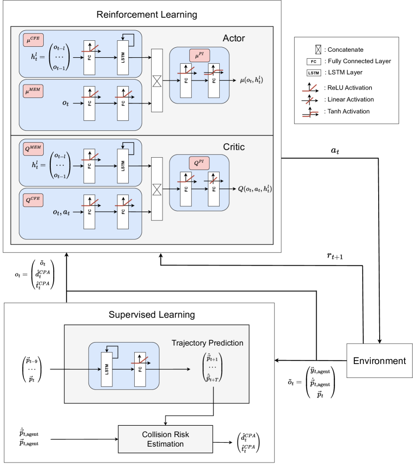
We showcase the potential of our two-step architecture (Step 1: CR estimation, Step 2: DRL) for handling DOA tasks, thereby underscoring its suitability for implementation inside a local path planning unit of a PPC modularization. More precisely, we define a traffic-type independent environment where an agent needs to avoid dynamic obstacles and quantify the advantage in terms of the reward difference of the proposal in comparison to a ’conventional’ DRL agent for obstacle avoidance. Figure 1 visualizes the architecture.
The paper is structured as follows: Section 2 provides a concise and formal problem description of the considered DOA task. Section 3 displays the estimation of the CR metrics, while the reinforcement learning (RL) environment and algorithms are presented in Section 4. Section 5 shows the results, and Section 6 concludes this article. The source code for this paper is publicly available at GitHub (Waltz and Paulig, 2022).
2 Problem description
We consider a two-dimensional DOA task detached from a specific transportation context. We define a point-mass agent with a constant longitudinal speed for simplification while the lateral acceleration can be controlled. Since this study aims at a realistic setting with non-linearly moving obstacles, we generically define an obstacle trajectory as:
| (1) |
where is the position of the obstacle at time step . The terms and denote the linear and non-linear components of the obstacle trajectory, respectively. More precisely, the linear part is defined as:
| (2) |
with the initial obstacle position and the constant, obstacle-dependent velocity . Equation (2) ensures that the obstacle moves in a specific direction. At the same time, the non-linear part can capture course deviations due to environmental effects or the obstacle’s own avoidance maneuvers. Importantly, different practical behaviors of obstacles can be simulated via different specifications of . Throughout this study, we exemplarily consider two different kinds of non-linear obstacle movements: stochastic and periodic trajectories.
Stochastic trajectories. The first non-linear specification is based on a stochastic two-dimensional auto-regressive process (Tsay, 2010):
| (3) |
with initial value , auto-regressive parameter , and variance of the centered noise stemming from the multivariate normal distribution. Addressing the noisy nature of the process, we perform an exponential smoothing of (3):
| (4) |
with the smoothing factor . Moreover, to account for different obstacle velocities, we scale the stochastic trajectory:
| (5) |
with maximum obstacle speed .
Periodic trajectories. The second obstacle behavior considered in this study incorporates a sinus pattern with additional noise:
| (6) |
with amplitude , period , and variance .
Figures 3 and 4 visualize examples of the stochastic and periodic trajectories, respectively, in blue color. Throughout this study, we use a simulation step size of for simulating obstacle and agent movement. Crucially, to train a collision risk estimator that estimates CR metrics for each obstacle and for each time step, we impose the following assumption:
Assumption 1: Behavior stability.
The behavior of the obstacles used to train the collision risk estimator is similar to the obstacle behavior in the simulation environment.
3 Step 1: Supervised learning
This section describes the supervised learning step of our approach as depicted in Figure 1. For each obstacle, we predict its future trajectory based on previous observations and compute the associated collision risk subsequently.
3.1 Basics
Supervised learning is the most common form of machine learning and describes the task of learning a mapping from potentially high-dimensional input samples to corresponding target vectors based on labeled data (LeCun et al., 2015; Zhou et al., 2021). Paired with (deep) neural networks as function approximators, supervised learning approaches have shown remarkable successes in various real-world problems such as speech recognition (Nassif et al., 2019) or object detection (Dhillon and Verma, 2020). In this study, we consider the regression task of having data pairs , where , , and learning the parameter vector of a neural network by minimizing the mean squared error with the Adam optimizer (Kingma and Ba, 2014).
3.2 Trajectory prediction
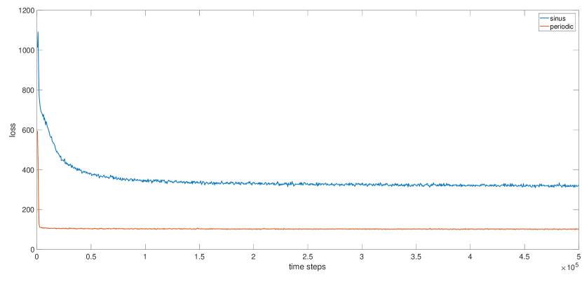
The input features contain information about previous positions of the obstacle , from which the neural network should approximate the next position . We construct the neural network with an LSTM-layer (Hochreiter and Schmidhuber, 1997) of 64 hidden units. The output is forwarded through another hidden layer with 64 neurons and ReLU activation to yield output in . The training progress of the network is depicted in Figure 2 for both defined non-linear obstacle movements.
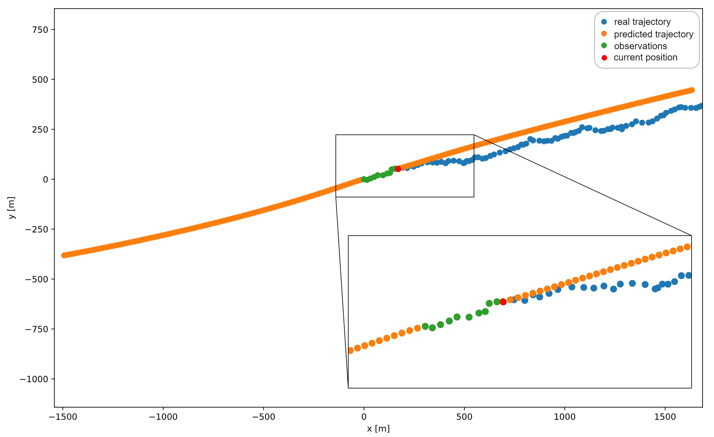
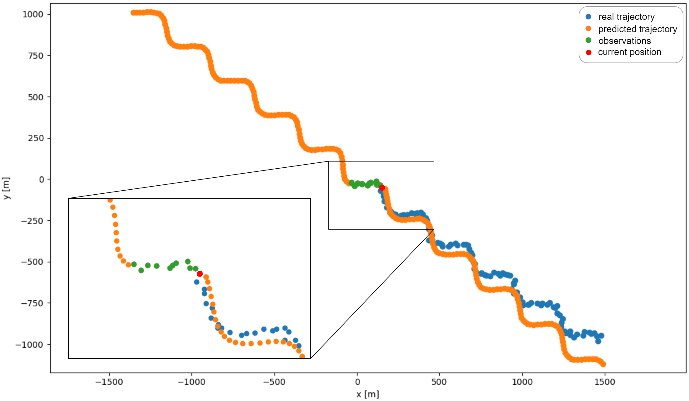
After the training is completed, we perform subsequent one-step-ahead forecasts to predict an obstacle’s entire trajectory for a time horizon . More precisely, we always take the last ten positions, possibly including predicted ones, to predict the following position iteratively. To illustrate the training results, we provide a representative example for a predicted trajectory in Figure 3 for the stochastic obstacle movement and Figure 4 for the periodic movement. The blue dots represent the ground truth trajectory, from which only the first ten dots, shown in green, are observed. These observations are used to iteratively compute the predicted trajectory, which is shown in orange. Since we assume that not all previous positions of an obstacle are observable, we predict past positions as well. These past obstacle positions are later used to estimate if the agent already passed and obstacle; see Section 3.3. Since the obstacle trajectories defined in (5) and (6) are symmetric, we can use the same model to predict past positions.
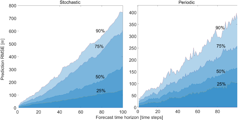
To quantitatively evaluate the prediction accuracy, we compute the root mean squared error (RSME) between predicted and real trajectories for both obstacle movements, as shown in Figure 5, with different quantiles. We can see that the prediction accuracy is relatively high for short-term predictions, but expectedly increases with increased forecasting time.
3.3 Collision risk estimation
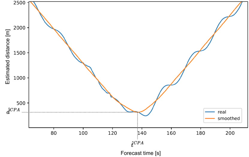
After predicting the trajectory of an obstacle for a time horizon , which equals a forecast time of based on a simulation step size of , we can estimate the CPA by numerically finding the minimum between the predicted obstacle and the predicted agent trajectory. For the agent, we thereby assume a linear movement based on its current velocity vector. An example is illustrated in Figure 6 for a periodic movement of the obstacle, where the blue curve represents the estimated distance between the agent and obstacle based on these predictions. Naturally, these distance estimates exhibit the periodic oscillations of the obstacle trajectory. To reduce the variance in the estimation of and caused by this pattern, we apply a symmetric moving average filter on the estimated distance:
where . The variables and denote the distance estimates between agent and obstacle at step before and after smoothing, respectively. The resulting estimates for and using the smoothed distance are depicted in orange color in Figure 6. Note that negative values for the are possible if the agent already passed the obstacle.
4 Step 2: Reinforcement Learning
4.1 Basics
RL aims at solving sequential decision tasks in which an agent interacts with an environment under the objective to maximize a numerical reward signal (Sutton and Barto, 2018). Formally, we consider Markov Decision Processes (MDP, Puterman 1994) consisting of a state space , an action space , an initial state distribution , a state transition probability distribution , a reward function , and a discount factor . At each time step , the agent receives a state information , selects an action , gets an instantaneous reward , and transitions based on the environmental dynamics to the next state . In practical applications, the full-state information is rarely available due to sensor limitations, delays, noise, or other disturbances. Addressing this issue, a generalization called Partially Observable Markov Decision Processes (POMDP, Kaelbling et al. 1998) introduces two additional components: the observation space and the observation function . In a POMDP, the agent does not receive the new state directly, but instead an observation , which is generated with probability by the observation function . Consequently, a POMDP is a Hidden Markov Model with actions and the observations are used for learning. In the following, we use capital notation, e.g., , to indicate random variables and small notation, e.g., or , to describe their realizations.
Objective of the agent in the MDP scenario is to optimize for a policy , a mapping from states to probability distributions over actions, that maximizes the expected return, which is the expected discounted cumulative reward, from the start state: . Common practice is the definition of action value functions , which are the expected return when starting in state , taking action , and following policy afterwards: . Crucially, in an MDP there is a deterministic optimal policy if the state space is finite or countably infinite (Puterman, 1994). The policy is connected with optimal action-values . The general control objective of RL is to find or approximate .
4.2 Recurrent reinforcement learning
As described in Section 4.1, only observations rather than full states are available in the POMDP case. One popular approach to handle this scenario is the construction of belief states, which are distributions over the real states the agent might be in, given the observation so far. This approach requires a model of the environment and is computationally demanding (Heess et al., 2015). An alternative approach might be to stack past observations together (Mnih et al., 2015), but this quickly increases the input dimension and limits the agent to a fixed number of frames. Finally, a further approach is to incorporate recurrency into the function approximators of model-free algorithms, which was shown to yield strong performances (Ni et al., 2021). The recurrency enriches the agent’s decision making by extracting information from past observations, potentially yielding an improved ability to solve problems without access to the complete state vector.
In this study, we follow the latter approach and use the LSTM-TD3 algorithm of Meng et al. (2021), which adds LSTM layers to the off-policy, actor-critic TD3 algorithm of Fujimoto et al. (2018). Crucially, the LSTM-TD3 uses a deterministic policy and defines the past history of length at time step defined as:
The zero-valued dummy observation is of the same dimension as a regular observation. Note that the definition of slightly differs from Meng et al. (2021) since we do not include past actions in the history. Furthermore, we set throughout the paper, analogous to the history length of the trajectory prediction from Section 3. The algorithm disassembles both actor and critic into different sub-components. Precisely, there is a memory extraction (MEM) part in the function approximators, and , respectively, that processes the history. In parallel, the current feature extraction (CFE) components and process the observation of the current step . Finally, the output of both MEM and CFE are concatenated and fed into the perception integration (PI) components and . These aggregate the extracted pieces of information and yield the final result. The network design of our LSTM-TD3 implementation is included in Figure 1 and formalized as follows:
where is the concatenation operator. The optimization of the algorithm is identical to the TD3. Moreover, to ensure the robustness of our architecture with respect to the algorithm, we apply the SAC algorithm of Haarnoja et al. (2018a, b), which uses a stochastic actor and automated tuning of the algorithm’s temperature parameter. We construct the network design analogous to the LSTM-TD3 networks and refer to the approach in the following as LSTM-SAC.
4.3 Training environment
We aim to develop a challenging training environment for DOA where the agent has to anticipate several obstacle trajectories to avoid collisions. To solely focus on the collision avoidance task and prevent the agent from making strategic decisions, we define an environment where obstacles should be passed in a predefined fashion, so-called passing rules. Moreover, research on RL-based DOA indicates that the final performance increases when the collision risk in training is high (Hart and Okhrin, 2022), which we consider appropriately.
We consider a set of obstacles , where is the total number of obstacles in the environment and the obstacle dynamics follow (1). We further define an agent with position and velocity at time step , where denotes a constant longitudinal velocity component. The RL agent controls the lateral velocity component via the lateral acceleration . Formally, the agent computes an action each time step that is mapped to the lateral acceleration:
where defines the maximal lateral acceleration for the agent. The agent receives an observation vector each time step , defined as:
| (7) |
where is the maximum speed and , , and denote the position, estimated , and estimated of the -th obstacle, respectively. Crucially, the estimates and are thereby computed using the supervised learning module introduced in Section 3. The constants , , and are used for scaling. Since the computation of and is demanding, we update those values only every 10th simulation step. We emphasize that (7) slightly abuses notation and contains information about all obstacles . Consequently, is of dimension .
The passing rule for each obstacle is indicated by the index within the observation vector. The first three observations are reserved for agent-related observations, the following observations are reserved for obstacles with passing rule ’right’, and the last for obstacles with passing rule ’left’. Within these blocks of the same passing rule, obstacles are sorted according to ascending estimated . To validate the proposed approach, we additionally configure a baseline agent with a reduced observation space, neglecting and , and with sorting the obstacles according to ascending euclidean distance to the agent.
Following recent RL literature (Silver et al., 2018), we aim to keep the reward function as simple as possible. Therefore, we penalize the agent only when passing an obstacle on the wrong side:
| (8) |
B provides details about the initialization of the agent and the obstacles and other environment configurations. Figure 7 exemplary depicts a time interval of a training episode, where blue and green colors refer to obstacles with different passing rules.
5 Results
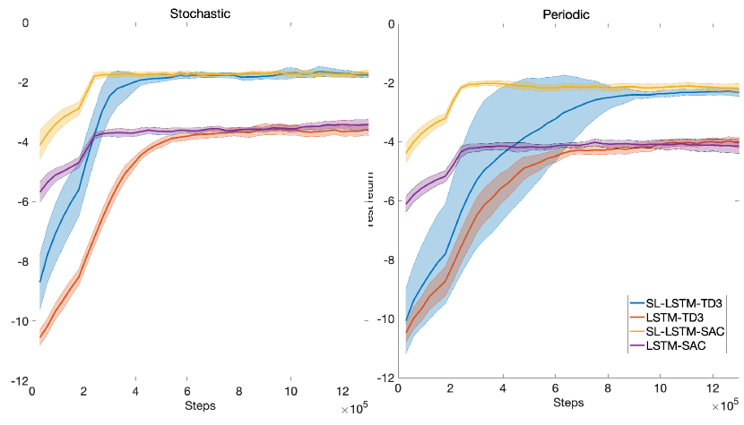
We compare our proposed two-step architecture with a training procedure without incorporating the estimates of and in the observation vector. Crucially, to demonstrate the proposal’s invariance to the selected DRL algorithm, we run the same experiments on two different actor-critic algorithms: the LSTM-TD3 of Meng et al. (2021), which uses a determinstic actor, and the LSTM-SAC as described in Section 4, which uses a stochastic actor. All experiments are conducted in the same training environment, which is described in Section 4.3. Hyperparameters shared by both algorithms are set equal; see Table 1. Figure 8 displays the training results, where we mark agents trained with CR estimates from the supervised learning module with the prefix ’SL’. The results are averaged over ten independent runs of each experiment, and we include point-wise confidence intervals for robustness.
Following (8), the absolute value of the test return of an episode can be immediately interpreted as the number of collisions. Thus, including the collision risk estimates based on supervised learning roughly halves the number of collisions. This performance boost is independent of the used algorithm. Notably, the high variance observed in the SL-LSTM-TD3 algorithm can be attributed to two out of the ten training runs, during which the training process remains stagnant for an extended period around an initial return value of -10.
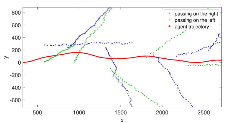
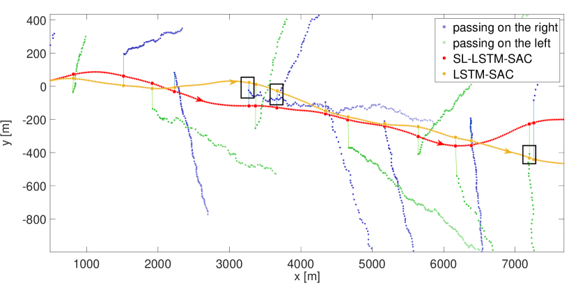
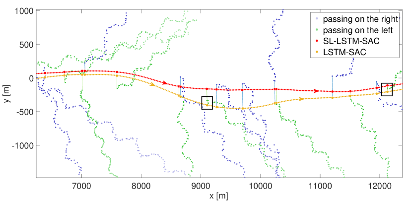
We visualize an exemplary episode for stochastic and periodic obstacle movements in Figures 9 and 10, respectively, to give further intuition about how the trained agents perform in the obstacle avoidance environment. Since both RL algorithms perform return-wise equally well, we show only the trajectory of the two configurations of the LSTM-TD3. The agent trajectories are depicted in red and yellow, and obstacle trajectories in blue and green, respectively, according to the imposed passing rules. The violations of the passing rules are marked with a black square. We can observe that the agent with the additional collision risk estimates (prefix ’SL’) chooses the better trajectory, resulting in no violation of passing rules. On the other hand, the baseline agent seems unable to accurately predict the trajectory of some obstacles, resulting in clear violations of passing rules.
6 Conclusion
Future sustainable transportation systems can benefit from autonomous vehicles in terms of safety and energy efficiency, particularly in non-lane-based domains such as air or maritime traffic. Such real-world autonomous systems necessitate robust local path planning capabilities, including the critical task of avoiding collisions with dynamic obstacles. This work proposes a two-step architecture that leverages recent advances from supervised learning and reinforcement learning. The first step captures non-linear movements of obstacles and estimates collision risk metrics in a supervised fashion, while the second step uses these estimates to enrich the observation space of an RL agent.
Our approach has demonstrated a significant enhancement in the collision avoidance capabilities of the respective autonomous agent, thereby constituting a valuable contribution to the realm of autonomous vehicles. Importantly, our learning architecture exhibits versatility by not being confined to a specific set of obstacle dynamics. In our upcoming research, we aim to validate this architecture using a diverse range of real-world obstacle behavior data and implementing it across different traffic domains. Moreover, the current approach focuses on providing point estimates of the collision risk with obstacles. In future work, we will consider the uncertainties connected with the collision risk estimates since these uncertainties are likely to be decision-relevant for real-life operations.
Acknowledgment
This work was partially funded by BAW - Bundesanstalt für Wasserbau (Mikrosimulation des Schiffsverkehrs auf dem Niederrhein). The authors are grateful to the Center for Information Services and High Performance Computing at TU Dresden for providing its facilities for high throughput calculations.
References
- Badue et al. (2021) Badue, C., Guidolini, R., Carneiro, R.V., Azevedo, P., Cardoso, V.B., Forechi, A., Jesus, L., Berriel, R., Paixao, T.M., Mutz, F., et al., 2021. Self-driving cars: A survey. Expert Systems with Applications 165, 113816.
- Bellemare et al. (2020) Bellemare, M.G., Candido, S., Castro, P.S., Gong, J., Machado, M.C., Moitra, S., Ponda, S.S., Wang, Z., 2020. Autonomous navigation of stratospheric balloons using reinforcement learning. Nature 588, 77–82.
- Brittain and Wei (2022) Brittain, M., Wei, P., 2022. Scalable autonomous separation assurance with heterogeneous multi-agent reinforcement learning. IEEE Transactions on Automation Science and Engineering 19, 2837–2848.
- Chun et al. (2021) Chun, D.H., Roh, M.I., Lee, H.W., Ha, J., Yu, D., 2021. Deep reinforcement learning-based collision avoidance for an autonomous ship. Ocean Engineering 234, 109216.
- Dhillon and Verma (2020) Dhillon, A., Verma, G.K., 2020. Convolutional neural network: a review of models, methodologies and applications to object detection. Progress in Artificial Intelligence 9, 85–112.
- Everett et al. (2018) Everett, M., Chen, Y.F., How, J.P., 2018. Motion planning among dynamic, decision-making agents with deep reinforcement learning, in: International Conference on Intelligent Robots and Systems, IEEE. pp. 3052–3059.
- Everett et al. (2021) Everett, M., Chen, Y.F., How, J.P., 2021. Collision avoidance in pedestrian-rich environments with deep reinforcement learning. IEEE Access 9, 10357–10377.
- Falanga et al. (2020) Falanga, D., Kleber, K., Scaramuzza, D., 2020. Dynamic obstacle avoidance for quadrotors with event cameras. Science Robotics 5, eaaz9712.
- Fawzi et al. (2022) Fawzi, A., Balog, M., Huang, A., Hubert, T., Romera-Paredes, B., Barekatain, M., Novikov, A., R Ruiz, F.J., Schrittwieser, J., Swirszcz, G., et al., 2022. Discovering faster matrix multiplication algorithms with reinforcement learning. Nature 610, 47–53.
- Feng et al. (2023) Feng, S., Sun, H., Yan, X., Zhu, H., Zou, Z., Shen, S., Liu, H.X., 2023. Dense reinforcement learning for safety validation of autonomous vehicles. Nature 615, 620–627.
- Fossen (2021) Fossen, T.I., 2021. Handbook of Marine Craft Hydrodynamics and Motion Control, 2nd Edition. John Wiley & Sons.
- Fujimoto et al. (2018) Fujimoto, S., Hoof, H., Meger, D., 2018. Addressing function approximation error in actor-critic methods, in: International Conference on Machine Learning, PMLR. pp. 1587–1596.
- Haarnoja et al. (2018a) Haarnoja, T., Zhou, A., Abbeel, P., Levine, S., 2018a. Soft actor-critic: Off-policy maximum entropy deep reinforcement learning with a stochastic actor, in: International Conference on Machine Learning, PMLR. pp. 1861–1870.
- Haarnoja et al. (2018b) Haarnoja, T., Zhou, A., Hartikainen, K., Tucker, G., Ha, S., Tan, J., Kumar, V., Zhu, H., Gupta, A., Abbeel, P., et al., 2018b. Soft actor-critic algorithms and applications. arXiv preprint arXiv:1812.05905 .
- Hart and Okhrin (2022) Hart, F., Okhrin, O., 2022. Enhanced method for reinforcement learning based dynamic obstacle avoidance by assessment of collision risk. URL: https://arxiv.org/abs/2212.04123, doi:10.48550/ARXIV.2212.04123.
- Heess et al. (2015) Heess, N., Hunt, J.J., Lillicrap, T.P., Silver, D., 2015. Memory-based control with recurrent neural networks. arXiv preprint arXiv:1512.04455 .
- Hochreiter and Schmidhuber (1997) Hochreiter, S., Schmidhuber, J., 1997. Long short-term memory. Neural computation 9, 1735–1780.
- Huang et al. (2020) Huang, Y., Chen, L., Chen, P., Negenborn, R.R., Van Gelder, P., 2020. Ship collision avoidance methods: State-of-the-art. Safety science 121, 451–473.
- International Maritime Organization (1972) International Maritime Organization, 1972. COLREG: Convention on the International Regulations for Preventing Collisions at Sea.
- Isufaj et al. (2022) Isufaj, R., Omeri, M., Piera, M.A., 2022. Multi-UAV conflict resolution with graph convolutional reinforcement learning. Applied Sciences 12, 610.
- Kaelbling et al. (1998) Kaelbling, L.P., Littman, M.L., Cassandra, A.R., 1998. Planning and acting in partially observable stochastic domains. Artificial Intelligence 101, 99–134.
- Kandepu et al. (2008) Kandepu, R., Foss, B., Imsland, L., 2008. Applying the unscented kalman filter for nonlinear state estimation. Journal of Process Control 18, 753–768.
- Kingma and Ba (2014) Kingma, D.P., Ba, J., 2014. Adam: A method for stochastic optimization. arXiv preprint arXiv:1412.6980 .
- Kuchar and Yang (2000) Kuchar, J.K., Yang, L.C., 2000. A review of conflict detection and resolution modeling methods. IEEE Transactions On Intelligent Transportation Systems 1, 179–189.
- LeCun et al. (2015) LeCun, Y., Bengio, Y., Hinton, G., 2015. Deep learning. Nature 521, 436–444.
- Lee et al. (2019) Lee, M.A., Zhu, Y., Srinivasan, K., Shah, P., Savarese, S., Fei-Fei, L., Garg, A., Bohg, J., 2019. Making sense of vision and touch: Self-supervised learning of multimodal representations for contact-rich tasks, in: International Conference on Robotics and Automation, IEEE. pp. 8943–8950.
- Lenart (1983) Lenart, A.S., 1983. Collision threat parameters for a new radar display and plot technique. The Journal of Navigation 36, 404–410.
- Li (2019) Li, Y., 2019. Reinforcement learning applications. arXiv preprint arXiv:1908.06973 .
- Liu et al. (2016) Liu, Z., Zhang, Y., Yu, X., Yuan, C., 2016. Unmanned surface vehicles: An overview of developments and challenges. Annual Reviews in Control 41, 71–93.
- Marin-Plaza et al. (2018) Marin-Plaza, P., Hussein, A., Martin, D., Escalera, A.d.l., 2018. Global and local path planning study in a ros-based research platform for autonomous vehicles. Journal of Advanced Transportation 2018.
- Meng et al. (2021) Meng, L., Gorbet, R., Kulić, D., 2021. Memory-based deep reinforcement learning for pomdps, in: International Conference on Intelligent Robots and Systems, IEEE. pp. 5619–5626.
- Meyer et al. (2020) Meyer, E., Robinson, H., Rasheed, A., San, O., 2020. Taming an autonomous surface vehicle for path following and collision avoidance using deep reinforcement learning. IEEE Access 8, 41466–41481.
- Mnih et al. (2015) Mnih, V., Kavukcuoglu, K., Silver, D., Rusu, A.A., Veness, J., Bellemare, M.G., Graves, A., Riedmiller, M., Fidjeland, A.K., Ostrovski, G., et al., 2015. Human-level control through deep reinforcement learning. Nature 518, 529–533.
- Mousavi et al. (2016) Mousavi, S.S., Schukat, M., Howley, E., 2016. Deep reinforcement learning: an overview, in: Proceedings of SAI Intelligent Systems Conference, Springer. pp. 426–440.
- Nassif et al. (2019) Nassif, A.B., Shahin, I., Attili, I., Azzeh, M., Shaalan, K., 2019. Speech recognition using deep neural networks: A systematic review. IEEE access 7, 19143–19165.
- Negenborn et al. (2023) Negenborn, R.R., Goerlandt, F., Johansen, T.A., Slaets, P., Valdez Banda, O.A., Vanelslander, T., Ventikos, N.P., 2023. Autonomous ships are on the horizon: here’s what we need to know. Nature 615, 30–33.
- Ni et al. (2021) Ni, T., Eysenbach, B., Salakhutdinov, R., 2021. Recurrent model-free RL is a strong baseline for many POMDPs. arXiv preprint arXiv:2110.05038 .
- Pandey et al. (2017) Pandey, A., Pandey, S., Parhi, D., 2017. Mobile robot navigation and obstacle avoidance techniques: A review. International Robotics & Automation Journal 2, 96–105.
- Polvara et al. (2018) Polvara, R., Sharma, S., Wan, J., Manning, A., Sutton, R., 2018. Obstacle avoidance approaches for autonomous navigation of unmanned surface vehicles. The Journal of Navigation 71, 241–256.
- Puterman (1994) Puterman, M.L., 1994. Markov Decision Processes: Discrete Stochastic Dynamic Programming. John Wiley & Sons.
- Rawson and Brito (2023) Rawson, A., Brito, M., 2023. A survey of the opportunities and challenges of supervised machine learning in maritime risk analysis. Transport Reviews 43, 108–130.
- Ribeiro et al. (2020) Ribeiro, M., Ellerbroek, J., Hoekstra, J., 2020. Review of conflict resolution methods for manned and unmanned aviation. Aerospace 7, 79.
- Sauer et al. (2018) Sauer, A., Savinov, N., Geiger, A., 2018. Conditional affordance learning for driving in urban environments, in: Conference on Robot Learning, PMLR. pp. 237–252.
- Silver et al. (2018) Silver, D., Hubert, T., Schrittwieser, J., Antonoglou, I., Lai, M., Guez, A., Lanctot, M., Sifre, L., Kumaran, D., Graepel, T., et al., 2018. A general reinforcement learning algorithm that masters chess, shogi, and go through self-play. Science 362, 1140–1144.
- Strickland et al. (2018) Strickland, M., Fainekos, G., Amor, H.B., 2018. Deep predictive models for collision risk assessment in autonomous driving, in: International Conference on Robotics and Automation, IEEE. pp. 4685–4692.
- Suárez-Varela et al. (2019) Suárez-Varela, J., Mestres, A., Yu, J., Kuang, L., Feng, H., Barlet-Ros, P., Cabellos-Aparicio, A., 2019. Feature engineering for deep reinforcement learning based routing, in: International Conference on Communications, IEEE. pp. 1–6.
- Sutton and Barto (2018) Sutton, R.S., Barto, A.G., 2018. Reinforcement Learning: An Introduction. Cambridge: The MIT Press.
- Treiber and Kesting (2013) Treiber, M., Kesting, A., 2013. Traffic Flow Dynamics: Data, Models and Simulation. Springer-Verlag Berlin Heidelberg.
- Tsay (2010) Tsay, R.S., 2010. Analysis of Financial Time Series. New Jersey: John Wiley & Sons.
- Vagale et al. (2021) Vagale, A., Oucheikh, R., Bye, R.T., Osen, O.L., Fossen, T.I., 2021. Path planning and collision avoidance for autonomous surface vehicles I: a review. Journal of Marine Science and Technology 26, 1292–1306.
- Vinyals et al. (2019) Vinyals, O., Babuschkin, I., Czarnecki, W.M., Mathieu, M., Dudzik, A., Chung, J., Choi, D.H., Powell, R., Ewalds, T., Georgiev, P., et al., 2019. Grandmaster level in starcraft II using multi-agent reinforcement learning. Nature 575, 350–354.
- Waltz and Okhrin (2023) Waltz, M., Okhrin, O., 2023. Spatial–temporal recurrent reinforcement learning for autonomous ships. Neural Networks 165, 634–653.
- Waltz and Paulig (2022) Waltz, M., Paulig, N., 2022. RL Dresden Algorithm Suite. https://github.com/MarWaltz/TUD_RL.
- Waltz et al. (2023) Waltz, M., Paulig, N., Okhrin, O., 2023. 2-level reinforcement learning for ships on inland waterways. arXiv preprint arXiv:2307.16769 .
- Wang et al. (2019) Wang, C., Wang, J., Shen, Y., Zhang, X., 2019. Autonomous navigation of uavs in large-scale complex environments: A deep reinforcement learning approach. IEEE Transactions on Vehicular Technology 68, 2124–2136.
- Xu et al. (2022) Xu, X., Lu, Y., Liu, G., Cai, P., Zhang, W., 2022. COLREGs-abiding hybrid collision avoidance algorithm based on deep reinforcement learning for usvs. Ocean Engineering 247, 110749.
- Zhang et al. (2020) Zhang, W., Feng, X., Goerlandt, F., Liu, Q., 2020. Towards a convolutional neural network model for classifying regional ship collision risk levels for waterway risk analysis. Reliability Engineering & System Safety 204, 107127.
- Zhao and Liu (2021) Zhao, P., Liu, Y., 2021. Physics informed deep reinforcement learning for aircraft conflict resolution. IEEE Transactions on Intelligent Transportation Systems 23, 8288–8301.
- Zheng et al. (2020) Zheng, K., Chen, Y., Jiang, Y., Qiao, S., 2020. A SVM based ship collision risk assessment algorithm. Ocean Engineering 202, 107062.
- Zhou et al. (2021) Zhou, X., Liu, H., Pourpanah, F., Zeng, T., Wang, X., 2021. A survey on epistemic (model) uncertainty in supervised learning: Recent advances and applications. Neurocomputing 489, 449–465.
Appendix A RL algorithm hyperparameters
| Hyperparameter | Value |
| Discount factor | 0.99 |
| Batch size | 32 |
| Loss function | Mean squared error |
| Replay buffer size | |
| Learning rate actor | |
| Learning rate critic | |
| Optimizer | Adam |
| History length | 10 |
| Number of units per hidden layer | 128 |
| Target noise† | 0.2 |
| Target noise clip† | 0.5 |
| Policy update delay† | 2 |
| Initial temperature* | 0.2 |
| Learning rate temperature* | 0.0001 |
Appendix B Environment details
At the beginning of a training episode, we initialize the agent’s dynamics to zero, except the longitudinal speed , that is sampled uniformly at random from the interval . The Euler and ballistic methods are used to update the agent’s lateral speed and the positions for the agent and obstacles at time step (Treiber and Kesting, 2013). Exemplary for the agent, we have:
| (9) | ||||
| (10) |
with corresponding to the simulation step size. One episode is defined as steps of updating.
For each obstacle, we define a passing rule. The set of obstacles that should only be passed, from the perspective of the agent, on the right side in the lateral direction is denoted as . Consequently, the remaining obstacles should be passed left and are denoted .
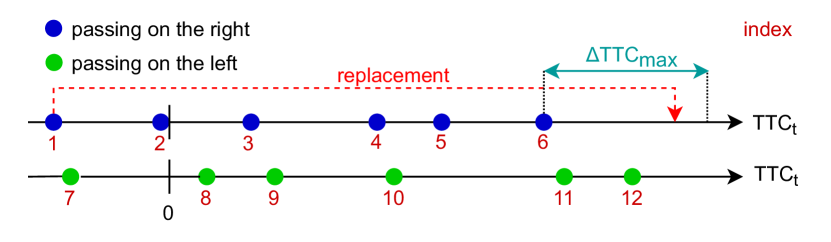
Next, a procedure to update the trajectories of obstacles needs to be defined so that the agent has to face threatening obstacles constantly. Therefore, we replace obstacles that have already been passed. To specify this condition, we introduced the helper variable as the agent’s time-to-collision with an obstacle in the longitudinal direction at time step , where the time-to-collision is computed based on the obstacle’s linear trajectory part (2). Negative values for relate to obstacles that have already passed the agent in the longitudinal direction. If for two obstacles holds: , , and , we replace obstacle as shown in Figure 11. Its new time-to-collision is randomly sampled from:
| (11) |
where is the maximal temporal distance for the new placement of an obstacle. This parameter affects the number of obstacles being passed in a certain time interval and is, therefore, a crucial design element of this environment. The same replacement procedure is applied for obstacles with passing rule ’left.’
Having computed the new value for for a replaced obstacle at time step , the new position and velocity need to be determined. First, we draw values for the constant velocity of the linear trajectory part from uniform distributions:
| (12) | ||||
| (13) |
Second, the new longitudinal position can be set as follows:
| (14) |
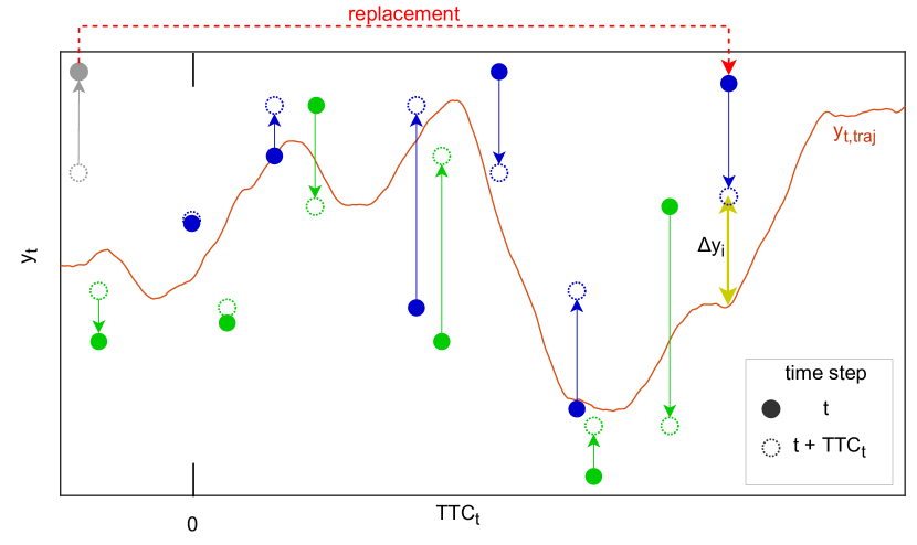
Third, having the lateral speed of the replaced obstacle set, we generate the new lateral position with the help of a predefined, stochastic trajectory , inspired by Meyer et al. (2020). This lateral trajectory is computed at the beginning of an episode and is based on a smoothed AR(1) process, whose parameters reflect the kinematics of the agent. Figure 12 shows a replacement situation identical to Figure 11 and illustrates how this trajectory is used to define the new lateral position for a replaced obstacle. One can think of this process as an exemplary trajectory the agent has to follow to avoid collisions with obstacles. In the following, we define the smoothed AR(1) process and give a detailed explanation of the replacement of an obstacle based on that process.
The AR(1) process is defined as:
| (15) |
with auto-regressive parameter and variance . The parameters have been designed to model a lateral trajectory the agent can approximately follow under acceleration and velocity constraints represented by and . To reduce the noise, we exponentially smooth the AR(1) process:
| (16) |
where defines the smoothing factor. Based on this trajectory and having already computed , , , and via (11), (12), (13), and (14), one more step is needed to set the new lateral position for a replaced obstacle at time step .
We define as the absolute difference between an obstacle’s lateral position and the defined trajectory when agent and obstacle are at the same longitudinal position ():
| (17) |
shown yellow in Figure 12. To force our agent to move approximately along the trajectory , the positional difference should be small, thus being another crucial design parameter to adjust the complexity of the environment. Every time an obstacle is replaced, the variable is sampled from a normal distribution:
| (18) |
and lower-bounded to :
| (19) |
By changing the parameters , , and , one can adjust how close the obstacles are coming to the trajectory when obstacle and agent are at the same longitudinal position. Table 2 contains the chosen values for those parameters. Finally, the lateral position for obstacles is computed via:
| (20) |
and for obstacles via:
| (21) |
Figure 12 shows the final lateral position and time-to-collision for a replaced obstacle as a filled circle. The linear trajectory part is represented as a blue or green arrow. Having defined the linear trajectory part of an obstacle, we can now add the non-linear trajectory part based on (1).
| Parameter | Description | Value |
| number of obstacles | 10 | |
| agent’s maximum lateral acceleration | ||
| agent’s maximum speed | ||
| simulation step size | ||
| number of episode steps | 500 | |
| scaling factor for observation | ||
| scaling factor for observation | ||
| scaling factor for observation | ||
| maximal temporal distance for replacing an obstacle | ||
| AR(1) process parameter | ||
| AR(1) process parameter | ||
| normal distribution variance | ||
| normal distribution variance | ||
| normal distribution variance | ||
| smoothing factor | ||
| smoothing factor | ||
| normal distribution mean | ||
| normal distribution variance | ||
| minimum bound for | ||
| periodic trajectory amplitude | ||
| periodic trajectory period |