Comparative analysis of phase-field and intrinsic cohesive zone models for fracture simulations in multiphase materials with interfaces: Investigation of the influence of the microstructure on the fracture properties

Abstract

This study evaluates four widely used fracture simulation methods, comparing their computational expenses and implementation complexities within the Finite Element (FE) framework when employed on heterogeneous solids. Fracture methods considered encompass the intrinsic Cohesive Zone Model (CZM) using zero-thickness cohesive interface elements (CIEs), the Standard Phase-Field Fracture (SPFM) approach, the Cohesive Phase-Field fracture (CPFM) approach, and an innovative hybrid model. The hybrid approach combines the CPFM fracture method with the CZM, specifically applying the CZM within the interface zone. The finite element model studied is characterized by three specific phases: Inclusions, matrix, and the interface zone. This case study serves as a potential template for meso- or micro-level simulations involving a variety of composite materials. The thorough assessment of these modeling techniques indicates that the CPFM approach stands out as the most effective computational model provided that the thickness of the interface zone is not significantly smaller than that of the other phases. In materials like concrete, which contain interfaces within their microstructure, the interface thickness is notably small when compared to other phases. This leads to the hybrid model standing as the most authentic finite element model, utilizing CIEs within the interface to simulate interface debonding. A significant finding from this investigation is that the CPFM method is in agreement with the hybrid model when the interface zone thickness is not excessively small. This implies that the CPFM fracture methodology may serve as a unified fracture approach for multiphase materials, provided the interface zone’s thickness is comparable to that of the other phases. In addition, this research provides valuable insights that can advance efforts to fine-tune material microstructures. An investigation of the influence of the interface material properties, morphological features and spatial arrangement of inclusions showes a pronounced effect of these parameters on the fracture toughness of the material.

1 Introduction

At the meso or micro level, materials are primarily composed of different phase constituents. For example, concrete at mesoscale can be characterized as a three-phase material comprising mortar matrix, inclusions, and a distinct interface phase known as Interfacial Transition Zone (ITZ). This zone encircles aggregate inclusions and has considerably inferior mechanical properties [1].

The nonlinear and complicated behavior of many engineering materials is due to their unique microstructural properties. Simulation of this complex behavior by macroscale numerical models often requires the integration of sophisticated material models equipped with numerous numerical parameters. Calibration of these parameters is a tedious process, and a major challenge arises when small changes in the microstructural properties of the material could make these carefully calibrated numerical parameters outdated, compromising the accuracy of macroscale simulations. Moreover, these macroscale simulations are not able to directly reproduce the initiation and progression of microcracks - an essential aspect for understanding material behavior at the structural level. To circumvent these problems and perform more physically representative simulations without an excessive number of numerical parameters, the solution lies in the use of small-scale simulations. Mesoscale or microscale simulations provide a path to more accurate and reliable modeling by focusing on the microstructural features inherent in the material. In many multiphase materials containing interfaces, cracks first initiate at the vulnerable interface region before progressing into the matrix. Hence, a reliable numerical model should accurately represent this process.

Numerous numerical techniques that capture this critical characteristic exist for modeling the onset and development of cracks in multiphase materials, especially those that are brittle or semi-brittle. In particular, the phase-field fracture method (PFM) [2, 3] and CZM [4, 5, 6] are two prominent and frequently used methods in this field.

The PFM is grounded in the principle of energy minimization. Crack initiation and propagation are determined by minimizing the total energy functional with respect to displacement and phase-field variables. This can be done either simultaneously or in a staggered approach. For comprehensive insights into the phase-field fracture approach and its implementation details, interested readers may refer to [7, 8, 9, 10, 11, 12, 13, 14]. A primary advantage of the PFM is its ability to track arbitrary crack paths within solids without the need for predefined potential damage zones. Furthermore, the quantitative capabilities of the PFM for accurately simulating force-displacement curves in complex structural mechanics problems have been demonstrated in [15]. Additionally, PFMs have been proven to be mesh-insensitive, provided that a sufficient number of elements are used within the diffused damage zone [16]. PFM shares these features with gradient-extended damage models. For a detailed comparison between these models, see [17]. Early versions of PFM demonstrated some shortcomings. These included a pronounced sensitivity of the simulated reaction-force displacement to the length-scale parameter, and a lack of integration of anisotropy and mode dependency in their formulations. Recent advancements in phase-field formulations, as detailed in [18, 19, 20], have successfully addressed the issue of length-scale sensitivity. Furthermore, the scope of PFM has been expanded to encompass both anisotropy and mode dependency [21, 22, 23, 24], as well as multiphysics problems [25, 26, 27, 28, 29, 30, 31, 32].

CZM is a popular technique for simulating fractures in brittle and semi-brittle materials, particularly those with significant heterogeneity. This modeling framework may be divided into two different categories: intrinsic and extrinsic approaches[33, 34]. Within the extrinsic framework, CIEs are integrated dynamically and simultaneously with the development of the simulation. In contrast, the intrinsic methodology requires the preemptive embedding of CIEs within the adjacent solid elements prior to the start of the simulation. Hence, the intrinsic approach is particularly effective in describing weak interfaces inherent in the structure of the material. For practical examples of CZM implementation in failure analysis of brittle and semi-brittle materials, as well as in multiphysics problems, readers may refer to [35, 36, 37, 38, 39, 40, 41, 42, 43, 44]. In this work the intrinsic approach is used to define the weak interfaces. Despite their effectiveness, the main drawback of intrinsic CZM is the necessity to predefine fracture zones. This requirement is not always straightforward, but in certain cases, such as the debonding of dissimilar materials or intergranular fracture, this approach proves quite effective [45]. It is worth mentioning that classical CZM, relying on a sharp interface approach, may encounter various numerical challenges. These issues include the balance of angular momentum, for which potential remedies can be found in the literature [46, 47, 48]. To address some of these shortcomings, an alternative formulation for the CZM, employing a diffuse or smeared approach, is also proposed [49, 50].

Recently, the PFM has gained popularity for simulating crack initiation and propagation in multiphase materials, especially those with an interface phase. These simulations concurrently address two phenomena: matrix cracking and interface debonding. Considering the approach used to address the interface in these simulations, they can be categorized into two main categories. In the first category, the interface is approximated using a finite width, and its failure is simulated with an auxiliary interface phase-field parameter [51, 52, 53, 54, 55, 56, 57, 58, 59, 60, 61, 62, 63, 64, 65]. In this approach, the interface fracture energy is either directly adopted from CZM or approximated through mathematical methods, which account for the influence of other phases on the interface’s fracture energy. In the second category, the interface is assumed to have zero thickness, and CIEs are utilized to simulate the interface debonding [66, 67, 68, 69, 70, 71, 72]. The main advantage of this approach is that it eliminates the need to approximate the interface width and solve for the auxiliary interface phase-field variable. However, the primary disadvantage is that this method requires pre-identifying the fracture zone in advance within the interface region. Figure 1 provides a summarized overview of the preceding discussion on various fracture approaches for the reader’s convenience.

Small-scale simulations encounter two main challenges: First, such simulations, especially for multiphase materials, can be computationally expensive. Considering the classical FE2 and the computational resources required, performing a small-scale simulation for each integration point of a macroscale simulation, proves to be extremely resource-intensive. Second, simulating the initiation and progression of cracks in these small-scale models significantly complicates the process, driving computational costs even higher. Considering these obstacles, it becomes crucial to select a numerical approach that minimizes complexity and reduces computational costs. However, in recent years, advancements such as off-line computational homogenization [73] have been introduced as remedies to accelerate the process.

This research work’s main innovative contribution lies in a comprehensive comparative study of four different numerical methods designed for simulating fracture in multiphase materials. The methods reviewed are: the cohesive zone model using CIEs, the standard phase-field fracture approach, the cohesive phase-field fracture method, and the hybrid model. The hybrid model is unique in its concurrent application of two fracture models: employing CZM for the interface debonding, while addressing the remaining phases with the CPFM approach. The evaluation of these methods is conducted through finite element simulations using a 2D benchmark model that features a single inclusion and consists of three distinct phases. This model serves as a potential reference for meso or microscale level simulations. The methods are assessed based on the complexity of implementation and computational cost associated with simulating crack initiation and propagation. A key assumption in this investigation is that the interface’s thickness is comparable to that of the other phases. Another innovative aspect of this work is a methodological study that highlights the role of interface mechanical properties and spatial distribution of inclusions in designing composites with enhanced fracture toughness. This research demonstrates that by employing the most effective numerical method identified, strategic placement of inclusions and proper modification of interface properties can effectively alter the direction of crack propagation. This alteration in the crack path leads to increased energy dissipation during a complete fracture. Such insights could significantly contribute to microstructural optimization, paving the way for the design of materials with superior fracture toughness.

Figure 1: Application of finite element methods for simulating fracture in heterogeneous materials: The hybrid fracture approach integrates CZM for interface debonding and PFM for matrix cracking.

2 Methods

This paper is structured as follows: Section 2 deals with the mathematical foundations of the phase-field fracture approach and cohesive zone modeling. Section 3 addresses the details of the numerical model, encompassing the benchmark three-phase numerical model employed in this research, material properties, element types, and boundary conditions. Section 4 assesses four numerical methods, examining their complexity of implementation and computational costs. Additionally, this section illustrates the performance of the most effective numerical approach in a 3D context and discusses a potential avenue for microstructure optimization. Finally, the Conclusions section concisely summarizes the principal findings of this study.

2.1 Phase-field fracture model for brittle fracture

The phase-field fracture methodology is characterized by the approximation of sharp cracks with diffused bands. In Figure 2, the area labeled as $\Omega$ is used to illustrate a diffused cracks. The width of this crack is determined by the length scale parameter $l_{c}$. As $l_{c}$ approaches zero, a reversion of the fracture to a sharp crack is observed [74]. Additionally, within Figure 2, $\Omega_{t}$ and $\Omega_{u}$ are denoted as Neumann and Dirichlet boundary conditions, respectively.

For a clearer understanding of the phase-field regularization of a sharp crack topology, a diffuse description of a one-dimensional crack at $x=0$ is presented in Figure 2, and is given as

$$\begin{cases}\phi_{1}(x)=\left(\frac{|x|}{2\,l_{c}}-1\right)^{2},\\ \phi_{2}(x)=e^{\frac{-|x|}{l_{c}}},\\ \phi_{3}(x)=1-\sin\left(\frac{|x|}{l_{c}}\right).\\ \end{cases}$$ (1)

The equations are constrained by the conditions

$$\phi(x=0)=1,\qquad\phi(x)\to 0:x\to\pm\infty.$$ (2)

Figure 2: The solid domain $\Omega$ is featuring a diffused crack, wherein the quantification of the diffused band’s width is provided through the utilization of the length scale parameter $l_{c}$. Furthermore, the approximation of a sharp crack topology by implementing various PFM approaches is illustrated.

In Figure 2, different formulations for $\phi(x)$ are represented, each corresponding to a different approximation of a sharp crack within various fracture approaches. These will be elaborated upon in the subsequent section.

Within the framework of the phase-field fracture concept, the symbol $\phi\in[0,1]$ is utilized to represent the degree of damage. Specifically, a value of $\phi=0$ corresponds to an undamaged material state, while a complete state of damage is signified by $\phi=1$. As indicated in Equation 3, it is imperative that the time derivative of the phase field damage parameter remains non-negative, ensuring the irreversibility of the induced damage, i.e.

$$\dot{\phi}(\mathbf{x},t)\geq 0.$$ (3)

Within the framework of the phase-field fracture method, the internal potential energy of the solid takes the form [75]

$$\psi(\bm{\varepsilon},\phi,\nabla_{\!\underaccent{\tilde}{x}}\phi)=\psi_{e}(\bm{\varepsilon},\phi)+\psi_{c}(\phi,\nabla_{\!\underaccent{\tilde}{x}}\phi).$$ (4)

where $\nabla_{\!\underaccent{\tilde}{x}}\bullet$ represents the spatial gradient of any scalar-valued field quantity $\bullet$, $\bm{\varepsilon}$ denotes the strain tensor pertaining to small deformations, $\psi_{e}$ denotes the stored strain energy, and $\psi_{c}$ represents the fracture surface energy. The determination of the stored strain energy is achieved through the relation

$$\psi_{e}(\bm{\varepsilon},\phi)=\omega(\phi)\,\psi_{0}(\bm{\varepsilon}),$$ (5)

where $\omega(\phi)$ represents the damage degradation function, responsible for reducing the stiffness of the undamaged material. The damage degradation function must adhere to the conditions

$$\omega(\phi=0)=1,\qquad\omega(\phi=1)=0,\qquad\omega^{\prime}(\phi=1)=0.$$ (6)

It is worth mentioning that the final constraint in Equation 6 is implemented to guarantee the convergence of damage in a fully damaged state, as highlighted in the study by [76]. Within Equation 5, $\psi_{0}$ represents the strain energy density function of the undamaged solid. For an isotropic elastic body, within a geometrically linear setting, the calculation of $\psi_{0}$ follows as

$$\psi_{0}(\bm{\varepsilon})=\frac{1}{2}\,\bm{\varepsilon}:\mathbb{E}_{0}:\bm{\varepsilon}=\frac{1}{2}\,\lambda_{0}\mathrm{tr}^{2}\,(\bm{\varepsilon})+\mu_{0}\,\bm{\varepsilon}:\bm{\varepsilon}=\frac{1}{2}\,\bm{\overline{\sigma}}:\mathbb{C}_{0}:\bm{\overline{\sigma}}=\psi_{0}(\bm{\overline{\sigma}}),$$ (7)

where $\mathbb{E}_{0}=2\mu_{0}\mathbb{I}_{0}+\lambda_{0}\bm{I}\otimes\bm{I}$ represents the fourth-order elastic stiffness tensor, $\lambda_{0}$ and $\mu_{0}$ are the Lamé constants, and $\mathbb{I}_{0}$ and $\bm{I}$ are the fourth-order and second-order identity tensors, respectively. In Equation 7, $\mathbb{C}_{0}=\mathbb{E}_{0}^{-1}$ represents the compliance tensor, $\bm{\overline{\sigma}=\mathbb{E}_{0}}:\bm{\varepsilon}$ is the effective stress tensor.

To mitigate the occurrence of cracking in regions subjected to compression, it is imperative to incorporate the damage degradation function in conjunction with the tension split of stored elastic energy such that

$$\psi(\bm{\varepsilon},\phi)=\omega(\phi)\,\psi_{0}^{+}(\bm{\varepsilon})+\psi_{0}^{-}(\bm{\varepsilon}).$$ (8)

Various alternatives are presented in the literature for this purpose. For instance, some of the most utilized methods include the anisotropic models of Lancioni and Royer-Carfagni [77], the anisotropic model proposed by Amor [78], and the anisotropic model developed by Miehe, Welschinger, and Hofacker [16]. In this research paper, the anisotropic model by Wu, Nguyen, and Zhou [79] is adopted for finite element simulation, wherein a positive/negative decomposition of the effective stress is considered. The fracture surface energy $\psi_{c}$ can be expressed as a volume integral via

$$\psi_{c}(\phi,\nabla_{\!\underaccent{\tilde}{x}}\phi)=\int_{\Gamma}G_{c}\,\mathrm{d}\Gamma\approx\int_{\Omega}G_{c}\gamma(\phi,\nabla_{\!\underaccent{\tilde}{x}}\phi)\,\mathrm{dA},$$ (9)

where $G_{c}$ represents the critical energy release rate, a parameter that characterizes the material’s fracture toughness. Additionally, $\gamma(\phi,\nabla_{\!\underaccent{\tilde}{x}}\phi)$ stands for the fracture surface density function. The calculation of $\gamma(\phi,\nabla_{\!\underaccent{\tilde}{x}}\phi)$ is achieved using the relation

$$\gamma(\phi,\nabla_{\!\underaccent{\tilde}{x}}\phi)=\frac{1}{c_{0}}\left[\frac{1}{l_{c}}\alpha(\phi)+l_{c}\nabla_{\!\underaccent{\tilde}{x}}\phi\cdot\nabla_{\!\underaccent{\tilde}{x}}\phi\right],$$ (10)

where $\alpha(\phi)$ is the crack geometric function, primarily employed to simulate the uniform evolution of the phase-field fracture parameter $\phi$. Additionally, the parameter $c_{0}$ is introduced to regularize $\psi_{c}(\phi,\nabla_{\!\underaccent{\tilde}{x}}\phi)$. It is essential that the crack geometric function $\alpha(\phi)$ must adhere to the conditions

$$\alpha(\phi=0)=0,\qquad\alpha(\phi=1)=1,\qquad\alpha^{\prime}(\phi)\geq 0.$$ (11)

As a result, the internal potential energy $\psi(\bm{\varepsilon},\phi,\nabla_{\!\underaccent{\tilde}{x}}\phi)$ takes the form

$$\psi(\bm{\varepsilon},\phi,\nabla_{\!\underaccent{\tilde}{x}}\phi)=\int_{\Omega}\omega(\phi)\,\psi_{0}(\bm{\varepsilon})\,\mathrm{dV}+\int_{\Omega}\frac{G_{c}}{c_{0}}\left[\frac{1}{l_{c}}\alpha(\phi)+l_{c}\nabla_{\!\underaccent{\tilde}{x}}\phi\cdot\nabla_{\!\underaccent{\tilde}{x}}\phi\right]\,\mathrm{dV}.$$ (12)

When evaluating the influence of externally applied loads on the solid domain denoted as $\Omega$, the computation of the external potential energy is undertaken as

$$P_{\mathrm{ext}}=\int_{\Omega}\bm{b^{*}}\cdot\bm{u}\,\mathrm{dV}+\int_{\partial\Omega}\bm{t^{*}}\cdot\bm{u}\,\mathrm{dA},$$ (13)

where $\bm{b^{*}}$ represents the volume forces, while $\bm{t^{*}}$ signifies the boundary forces. Consequently, the total potential energy of the solid domain is expressed as

$$P_{\mathrm{total}}=\int_{\Omega}\omega(\phi)\,\psi_{0}(\bm{\varepsilon})\,\mathrm{dV}+\int_{\Omega}\frac{G_{c}}{c_{0}}\left[\frac{1}{l_{c}}\alpha(\phi)+l_{c}\,\nabla_{\!\underaccent{\tilde}{x}}\phi\cdot\nabla_{\!\underaccent{\tilde}{x}}\phi\right]\,\mathrm{dV}-\int_{\Omega}\bm{b^{*}}\cdot\bm{u}\,\mathrm{dV}-\int_{\Omega}\bm{t^{*}}\cdot\bm{u}\,\mathrm{dA}.$$ (14)

The total energy functional represented by Equation 14 is characterized as being quadratic and convex. Consequently, through the minimization of $P_{\text{total}}$, it is feasible to determine the displacement and phase-field fracture parameters denoted as $(\bm{u},\phi)$ in a staggered manner. Within this model, crack propagation arises as a consequence of the interplay between the bulk and surface terms contained in $P_{\text{total}}$ according to

$$(\bm{u},\phi)=\mathrm{Arg}\{\mathrm{min}\,P_{\mathrm{total}}(\bm{u},\phi)\}\quad\text{subjected to}\quad\dot{\phi}\geq 0\quad\text{,}\quad\phi\in[0,1].$$ (15)

On one hand, under the influence of applied loads, the bulk elastic energy within the solid domain increases. Upon reaching a specific threshold, the system exhibits a preference for energy dissipation by incrementally elevating the phase-field fracture variable towards unity. Consequently, an increase in $\phi$ towards unity signifies the creation of two new crack surfaces, which in turn amplifies the system’s energy, as exemplified in Equation 14.

Through implementation of the first variation of the total energy functional and the application of the divergence theorem, the strong form of the displacement field of the phase-field fracture model takes the form

$$\begin{cases}\nabla\cdot\bm{\sigma}+\bm{b^{*}}=0,&\text{}\\ \bm{u}=\bm{u}_{0}&\text{on $\partial\Omega_{u}$,}\\ \bm{\sigma}\cdot\bm{n}=\bm{t}&\text{on $\partial\Omega_{t}$}.\\ \end{cases}$$ (16)

By employing thermodynamic principles and taking into account Equation 8, the Cauchy stress tensor $\bm{\sigma}$ follows for the standard relation

$$\bm{\sigma}=\frac{\partial\psi}{\partial\bm{\varepsilon}}.$$ (17)

The strong form for the phase-field variable reads

$$\begin{cases}\displaystyle Y-G_{c}\left[\frac{\partial\gamma(\phi,\nabla_{\!\underaccent{\tilde}{x}}\phi)}{\partial\phi}-\nabla_{\!\underaccent{\tilde}{x}}\cdot\left(\frac{\partial\gamma(\phi,\nabla_{\!\underaccent{\tilde}{x}}\phi)}{\partial\nabla_{\!\underaccent{\tilde}{x}}\phi}\right)\right]=0&\text{if}\quad\dot{\phi}>0,\\[21.52771pt] \displaystyle Y-G_{c}\left[\frac{\partial\gamma(\phi,\nabla_{\!\underaccent{\tilde}{x}}\phi)}{\partial\phi}-\nabla_{\!\underaccent{\tilde}{x}}\cdot\left(\frac{\partial\gamma(\phi,\nabla_{\!\underaccent{\tilde}{x}}\phi)}{\partial\nabla_{\!\underaccent{\tilde}{x}}\phi}\right)\right]<0&\text{if}\quad\dot{\phi}=0,\\ \end{cases}$$ (18)

where $Y$ is called energetic crack driving force and is determined from

$$Y=-\frac{\partial\psi}{\partial\phi}=-\omega{{}^{\prime}}(\phi)\frac{\partial\psi}{\partial\omega(\phi)}.$$ (19)

2.1.1 Standard phase-field fracture model

In the context of SPFM methodologies, the AT1 and AT2 models represent two distinct formulations commonly employed for the computational simulation of material fracture behavior. Both models aim to numerically capture the initiation and subsequent propagation of cracks within the material domain, but utilizing divergent mathematical frameworks. The AT1 model was introduced by Pham et al. [80], while the AT2 model was developed in works by Bourdin et al. [3] and Miehe et al. [16]. The damage degradation function in SPFM approaches is expressed as

$$\omega(\phi)=(1-\phi)^{2}+k,$$ (20)

where $k$ is a numerically small number responsible for conditioning the solution.

In the SPFM, the crack geometric function is formulated according to

$$\begin{cases}\alpha(\phi)=\phi&\text{for AT1 model,}\\[10.0pt] \alpha(\phi)=\phi^{2}&\text{for AT2 model.}\\ \end{cases}$$ (21)

Considering Equation 10, the parameter $c_{0}$ is calculated from

$$c_{0}=4\int_{0}^{1}\sqrt{\alpha(x)}\,\mathrm{dx},$$ (22)

where upon incorporating the respective crack geometric functions into Equation (22), the resultant values for $c_{0}$ are found to be 8/3 for the AT1 model and 2 for the AT2 model.

2.1.2 Cohesive phase-field fracture model

The primary distinction between standard phase-field fracture and cohesive phase-field fracture lies in the manner in which fracture energy is liberated. In standard phase-field fracture, once a threshold value is attained, fracture energy is instantaneously dissipated, whereas in cohesive phase-field fracture, this energy is released gradually and progressively over time.

The CPFM methodology employed in this investigation was originally introduced by [18, 19, 49] and is also suitable for modeling the failure behavior of quasi-brittle materials such as concrete. Notably, the cohesive phase-field fracture approach is distinguished by its insensitivity to the length-scale parameter $l_{c}$, marking a key feature of this fracture modeling technique.

The damage degradation function within the CPFM framework is represented as

$$\omega(\phi)=\frac{(1-\phi)^{2}}{(1-\phi)^{2}+a_{1}\,\phi+a_{1}\,a_{2}\,\phi^{2}+a_{1}\,a_{2\,}a_{3}\,\phi^{3}},$$ (23)

where the coefficients $a_{1}$, $a_{2}$ and $a_{3}$ are calculated as

$$\begin{cases}\displaystyle a_{1}=\frac{2\,E\,G_{c}}{\sigma_{u}^{2}\,\pi\,l_{c}},&\text{}\\[4.30554pt] \displaystyle a_{2}=2\left(-2\,k_{0}\frac{G_{c}}{\sigma_{u}^{2}}\right)^{\frac{2}{3}}-\left(p+\frac{1}{2}\right),\\[4.30554pt] \displaystyle a_{3}=\begin{cases}\displaystyle 0&\text{if \quad$p>0$,}\\[4.30554pt] \displaystyle\frac{1}{a_{2}}\left[\frac{1}{8}\left(\frac{d_{u}\,\sigma_{u}}{G_{c}}\right)^{2}-(1+a_{2})\right]&\text{if \quad$p=0$,}\end{cases}&\text{}\\ \end{cases}$$ (24)

where $E$ is the module of elasticity and $p$ corresponds to an exponent that is determined by the inherent material properties. Additionally, $k_{0}$ represents the initial slope, while $d_{u}$ signifies the ultimate crack opening value on the material’s softening curve.

The crack geometric function in CPFM model is expressed as

$$\alpha(\phi)=2\phi-\phi^{2},$$ (25)

which leads to $c_{0}=4\int_{0}^{1}\sqrt{\alpha(x)}\,\mathrm{dx}=\pi$ within the CPFM modeling approach.

The history variable is defined as

$$\begin{cases}\displaystyle H(\bm{x},t)=\max\left\{\psi_{\mathrm{eq}}^{0},\max\psi_{\mathrm{eq}}(\bm{\varepsilon}(x,t))\right\},\\ \displaystyle\psi_{\mathrm{eq}}^{0}=\frac{1}{2E}\sigma_{u}^{2},\end{cases}$$ (26)

where $\psi_{\mathrm{eq}}^{0}$ acts as a threshold value that determines the onset of damage initiation within the material.

Table 5 provides a concise summary of the distinctions between the SPFM and CPFM approaches. Additionally, Figure 3 displays the illustrations of the crack geometric function for various phase-field fracture formulations.

$$\begin{cases}\frac{G_{c}}{c_{0}}(2l_{c}\nabla\phi-\frac{a^{\prime}(\phi)}{l_{c}})-\omega^{\prime}(\phi)H=0&\text{}\\ \nabla\phi.n=0&\text{on $\Gamma$}\\ \end{cases}$$ (27)

Figure 3: Crack geometric functions for different phase-field fracture schemes.

In this study, cohesive zone model, AT2 model from the standard phase-field fracture, cohesive phase-field fracture model, and an innovative hybrid model are used to investigate crack initiation and propagation in a multiphase material with interface. In the hybrid formulation, cohesive zone model is used for interface debonding and the cohesive phase-field fracture approach is utilized for matrix cracking.

Table 1: Comparison between standard and cohesive phase field fracture.

Parameters	Standard phase-field fracture	Cohesive phase-field fracture
$\phi(x)$	$\begin{cases}\phi(x)=\left(\frac{|x|}{2l_{c}}-1\right)^{2}&\text{AT1 model}\\ \phi(x)=\mathrm{exp}(\frac{-|x|}{l_{c}})&\text{AT2 model}\\ \end{cases}$	$\phi(x)=1-\sin\left(\frac{|x|}{l_{c}}\right)$
$\alpha(\phi)$	$\begin{cases}\alpha(\phi)=\phi&\text{AT1 model}\\ \alpha(\phi)=\phi^{2}&\text{AT2 model}\\ \end{cases}$	$\alpha(\phi)=2\phi-\phi^{2}$
$\omega(\phi)$	$\omega(\phi)=(1-\phi)^{2}+k$	$\omega(\phi)=\frac{(1-\phi)^{2}}{(1-\phi)^{2}+a_{1}\phi+a_{1}a_{2}\phi^{2}+a_{1}a_{2}a_{3}\phi^{3}}$
$c_{0}$	$\begin{cases}c_{0}=\frac{8}{3}&\text{AT1 model}\\ c_{0}=2&\text{AT2 model}\\ \end{cases}$	$c_{0}=\pi$
$H(x,t)$	$H(\mathbb{x},t)=\max\left\{\max\psi_{\mathrm{eq}}(\bm{\varepsilon}(x,t))\right\}$	$\begin{cases}H(\mathbb{x},t)=\max\left\{\psi_{\mathrm{eq}}^{0}\ ,\max\psi_{\mathrm{eq}}(\bm{\varepsilon}(x,t))\right\}&\text{}\\ \psi_{\mathrm{eq}}^{0}=\frac{1}{2E}\sigma_{u}^{2}&\text{}\\ \end{cases}$

2.2 Cohesive zone model

Originally proposed by Barenblatt [81, 5], the cohesive zone model focuses on the material behavior within a zone immediately preceding a traction-free crack tip, commonly termed the cohesive zone or fracture process zone (FPZ). Barenblatt referred to the FPZ as the terminal region, noting that due to the proximity of the crack surfaces, significant interatomic forces arise, whose magnitude depends on the relative displacements of the surfaces.

Figure 4: Three distinct sets of cohesive elements are generated at various phases: within the matrix, inside the inclusion, and in the interface Zone[82].

Numerically, the implementation of the CZM within a finite element framework can be approached in several ways. One method involves the duplication of common nodes at interfaces between adjacent solid elements, thereby creating a new cohesive interface element. This technique is known as the segment-to-segment interface finite element method. Alternatively, there exists the node-to-segment approach, which offers a different perspective on interface element formulation. For a comprehensive understanding of these methodologies, interested readers are directed to explore the detailed exposition in [46], which provides an in-depth analysis of both approaches. CIEs are assigned a Traction-Separation law (TSL) to simulate crack initiation and propagation. For an in-depth exploration of the cohesive zone model in highly heterogeneous materials, readers are referred to [82]. Figure 4 offers a schematic representation of a discretized multiphase finite element model equipped with cohesive zone elements.

2.3 Constitutive equations of Cohesive interface elements

In 1976, Hillerborg [83] introduced the first cohesive crack model for simulating discrete fractures in concrete’s fracture process zone. The TSL express the FPZ’s mechanical behavior, linking cohesive element traction to relative surface displacement. Various TSLs have been formulated for different engineering materials, generally comprising two segments: a pre-damage functional relationship and a post-initiation softening zone. These segments are seperated by a threshold stress, $\sigma_{\mathrm{max}}$, beyond which damage initiates. The TSL for mode-I and mode-II fracture can be represented respectively as [84]:

$$\begin{cases}\displaystyle\sigma_{n}=f_{n}(\delta_{n}),\\ \displaystyle\sigma_{t}=f_{s}(\delta_{s}),\end{cases}$$ (28)

where $\sigma_{\mathrm{n}}$ and $\sigma_{\mathrm{t}}$ represent normal and shear traction, respectively, and $\delta_{n}$ and $\delta_{s}$ are crack opening displacement in normal and shear directions, respectively. In Equation (28), f shows the nonlinear function between traction and crack displacement.

In instances of multiaxial loading or geometries favoring multiple fracture modes, crack tips exhibit mixed-mode fracture states. Despite tensile loading condition in the studied benchmark model in this study, material heterogeneities induce mixed-mode crack propagation. Consequently, the corresponding TSL are employed in finite element simulations [84]. Given its simplicity and widespread application in modeling heterogeneous materials like composites, a bilinear TSL is adopted for each fracture mode in this work. Characterizing a bilinear TSL requires three parameters: cohesive element penalty stiffness K, threshold stress $\sigma_{\mathrm{max}}$, and critical fracture energy $G_{\mathrm{C}}$. The fracture energy follows from

$$G_{C}=\int_{0}^{\delta_{f}}\sigma\,\mathrm{d}\delta \text{for}\quad 0\leq\delta\leq\delta_{f}.$$ (29)

Before the initiation of damage, the normal and shear stress can be calculated as

$$\begin{cases}\displaystyle\sigma_{n}=k_{n0}\left\langle\delta_{n}\right\rangle,&\text{(normal direction)}\\ \displaystyle\sigma_{t}=k_{s0}\,\delta_{s},&\text{(shear direction)}\end{cases}$$ (30)

where $k_{\mathrm{n0}}$ and $k_{\mathrm{s0}}$ are the penalty stiffness in normal and shear directions, respectively. The symbol $\left\langle\bullet\right\rangle$ used in Equation (30) represents the Macaulay bracket. The Macaulay bracket indicates that compressive deformation or stress states do not initiate damage in the model. A quadratic stress damage criterion is used for damage initiation. Damage is presumed to commence when the function involving nominal stress ratios attains a value of one

$$\left(\frac{\left\langle\ \sigma_{\mathrm{n}}\right\rangle}{\sigma_{\mathrm{n}}^{0}}\right)^{2}+\left(\frac{\sigma_{\mathrm{s}}}{\sigma_{\mathrm{s}}^{0}}\right)^{2}=1,$$ (31)

where $\sigma_{n}^{0}$ and $\sigma_{s}^{0}$ are the tensile and shear cohesive strength, respectively. In FE simulations, when Equation (31) is satisfied and applied displacement increases, both normal and shear stress diminish, signifying the onset of the softening region. A scalar damage variable D is employed to quantify this stiffness degradation, encapsulating all damage mechanisms. D monotonically evolves from 0 to 1, reaching 1 upon complete failure. The normal and shear stress in the softening region are calculated via

$$\begin{cases}\displaystyle\sigma_{n}=(1-D)\,k_{n0}\left\langle\delta_{n}\right\rangle&\text{(normal direction)},\\ \displaystyle\sigma_{t}=(1-D)\,k_{s0}\,\delta_{s}&\text{(shear direction)}.\end{cases}$$ (32)

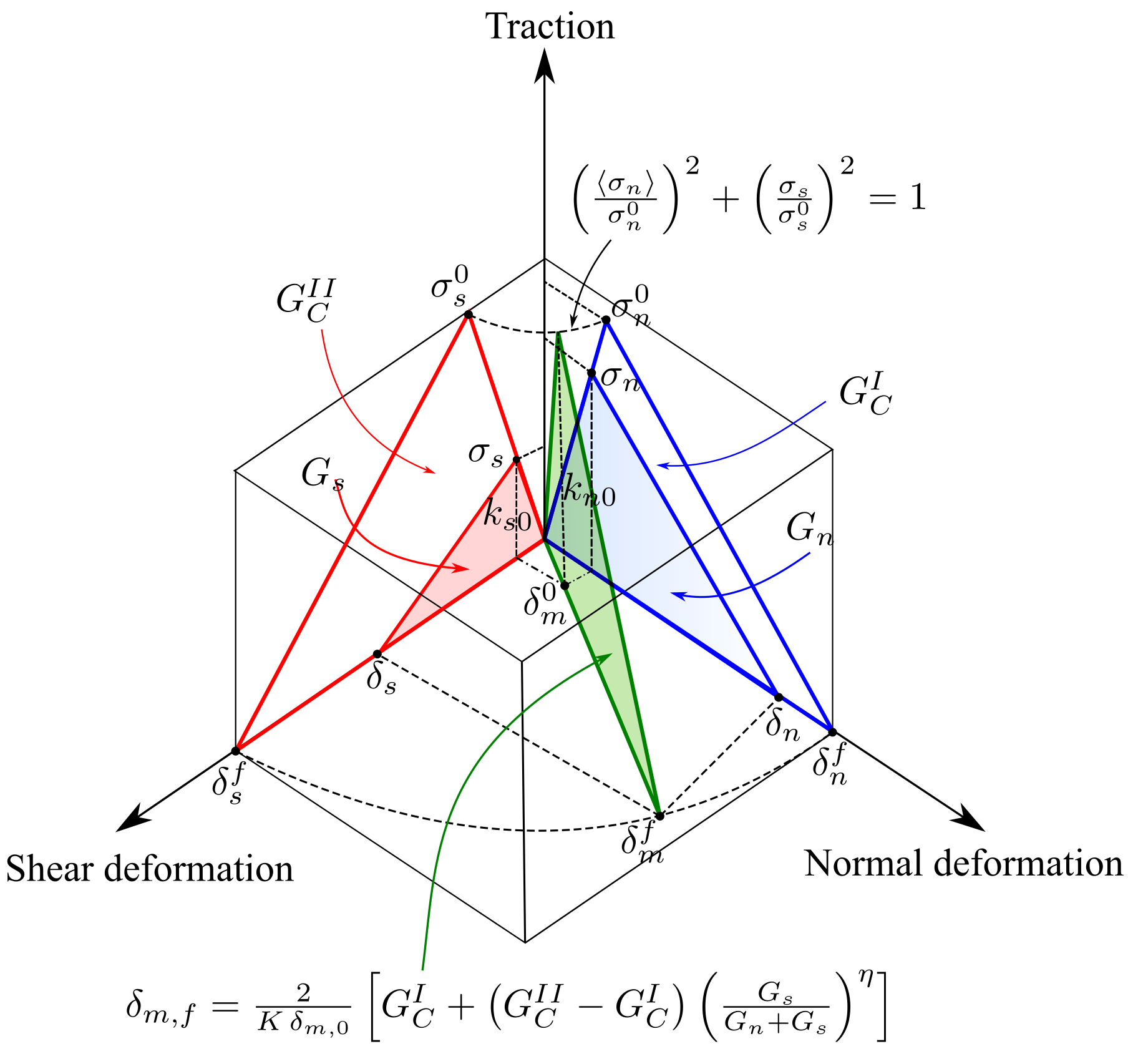
Figure 5: The quadratic nominal stress criterion and mixed-mode fracture criterion [82].

In the case of linear softening, the evolution of the damage variable D is computed using the expression proposed by [85], i.e.

$$D=\frac{\delta_{\mathrm{m}}^{f}(\delta_{\mathrm{m}}^{\mathrm{max}}-\delta_{\mathrm{m}}^{o})}{\delta_{\mathrm{m}}^{\mathrm{max}}(\delta_{\mathrm{m}}^{\mathrm{f}}-\delta_{\mathrm{m}}^{o})}.$$ (33)

In this context, $\delta_{m}^{0}$ and $\delta_{m}^{f}$ correspond to the effective displacements at the onset of damage and at complete failure, respectively. $\delta_{m}^{max}$ indicates the peak effective displacement throughout the loading history. The effective displacements in Equation (33) are computed using an expression suggested by [85] as

$$\delta_{m}=\sqrt[]{\left\langle\delta_{n}\right\rangle^{2}+\delta_{s}^{2}}.$$ (34)

The B-K fracture criterion [86] is employed for capturing mixed-mode fractures in composites and quasi-brittle materials. According to the B-K criterion, the effective displacement at complete failure is computed as

$$\delta_{m,f}=\frac{2}{K\delta_{m,0}}\Big{[}G_{C}^{I}+(G_{C}^{II}-G_{C}^{I})\Big{(}\frac{G_{s}}{G_{n}+G_{s}}\Big{)}^{\eta}\Big{]},$$ (35)

where $G_{C}^{I}$ and $G_{C}^{II}$ are the mode-I and mode-II fracture energies, respectively, while $G_{n}$ and $G_{s}$ quantify the work from tractions and corresponding displacements in normal and shear directions, respectively. According to [85], the $\eta$ value is typically set to 1.2 for quasi-brittle materials. As indicated by Equation 35, mixed-mode fracture energy varies based on Mode-I and Mode-II contributions. Figure 5 schematically illustrates this criterion. This paper utilizes finite element simulations with bilinear TSL to define the cohesive zone model. The quadratic stress damage criterion ascertains damage initiation, and a scalar damage variable $D$ describes damage evolution in the softening region. To capture mixed-mode fractures in composites and quasi-brittle materials, the B-K criterion is invoked.

Readers interested on further details about the implementation of the cohesive zone model formulation in the context of finite element analysis are referred to [87].

3 Finite Element Modeling

After creating the 2D model, the model is discretized using the mesh module of Abaqus/CAE. The geometry is a multiphase material with three different components, e.g. interface zone, matrix and inclusions. An essential consideration of the meshing process is that it is important to maintain continuity between the element surfaces. For the CZM simulation, free meshing technique with three-node triangular elements (CPS3) is used to discretize the model. The reason for this choice is that the CZM model is mesh dependent and triangular elements allow for more realistic crack propagation paths. After discretizing the model, the FE mesh file is imported and processed by in-hause algorithms in order to generate cohesive interface elements in different zones. Interested readers are referred to [82] to gain a deeper understanding of the CZM approach and of algorithms for inserting CIEs in multiphase materials. For the phase-field fracture simulations, square elements with four nodes are used to discretize the model. Similar to the CZM model, an important aspect is to maintain continuity between the element surfaces in the different phases of the material. In the present study, the interface thickness is designated as 0.6 mm. Figure 6(a) depicts the geometrical characteristics and dimensions of the 2D single inclusion investigated in this study. Additionally, it is imperative to discretize the interface zone in a manner that generates a minimum of four elements within the thickness direction, ensuring that the phase-field damage is adequately diffused within this zone. In the present research, all 2D samples are subjected to a displacement of 0.05 mm in x-direction. Figure 6(b) depicts the boundary conditions applied in the finite element simulations. Furthermore, a mesh size with an average element edge length of 0.15 mm is chosen for discretizing the model in both cohesive zone modeling and phase-field fracture simulations. A representation of the mesh configuration employed for both simulation is provided in Figure 7.

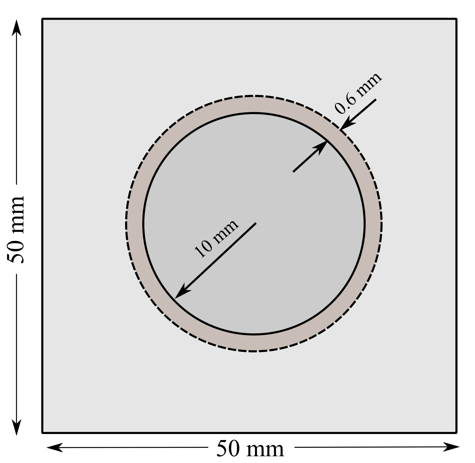
(a)

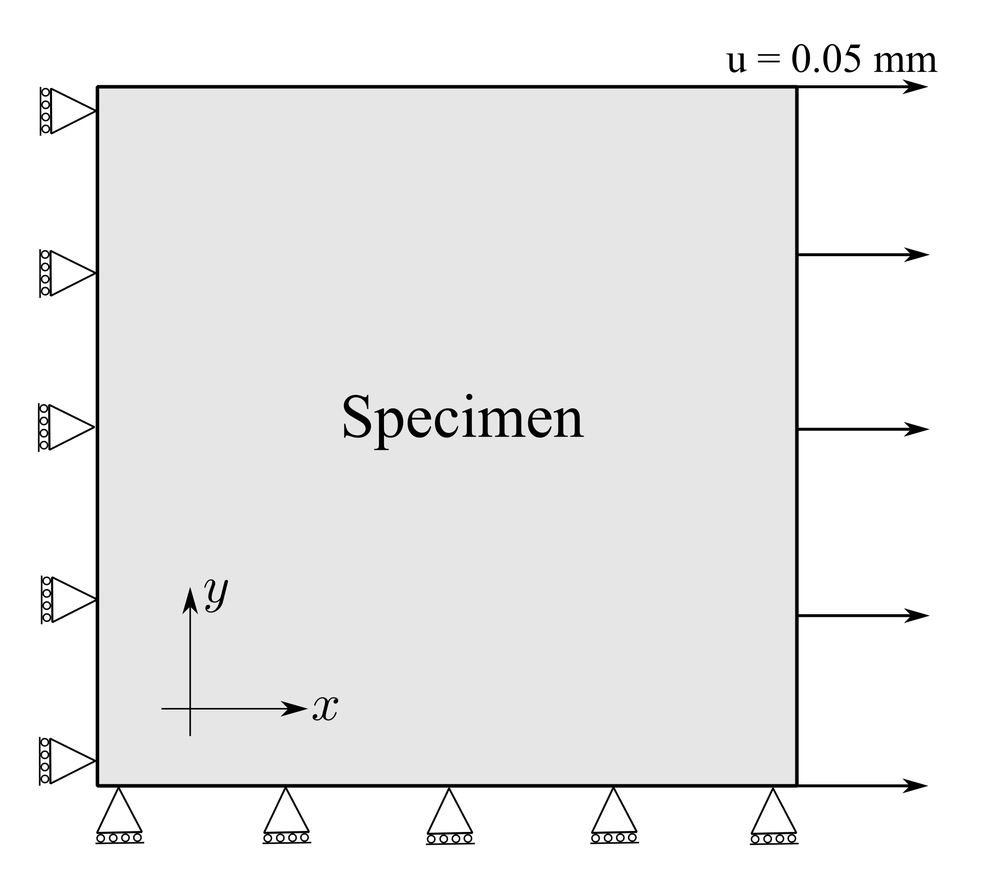
(b)

Figure 6: (a) Geometrical features of the 2D single inclusion benchmark model (b) and the boundary conditions applied in finite element simulations.

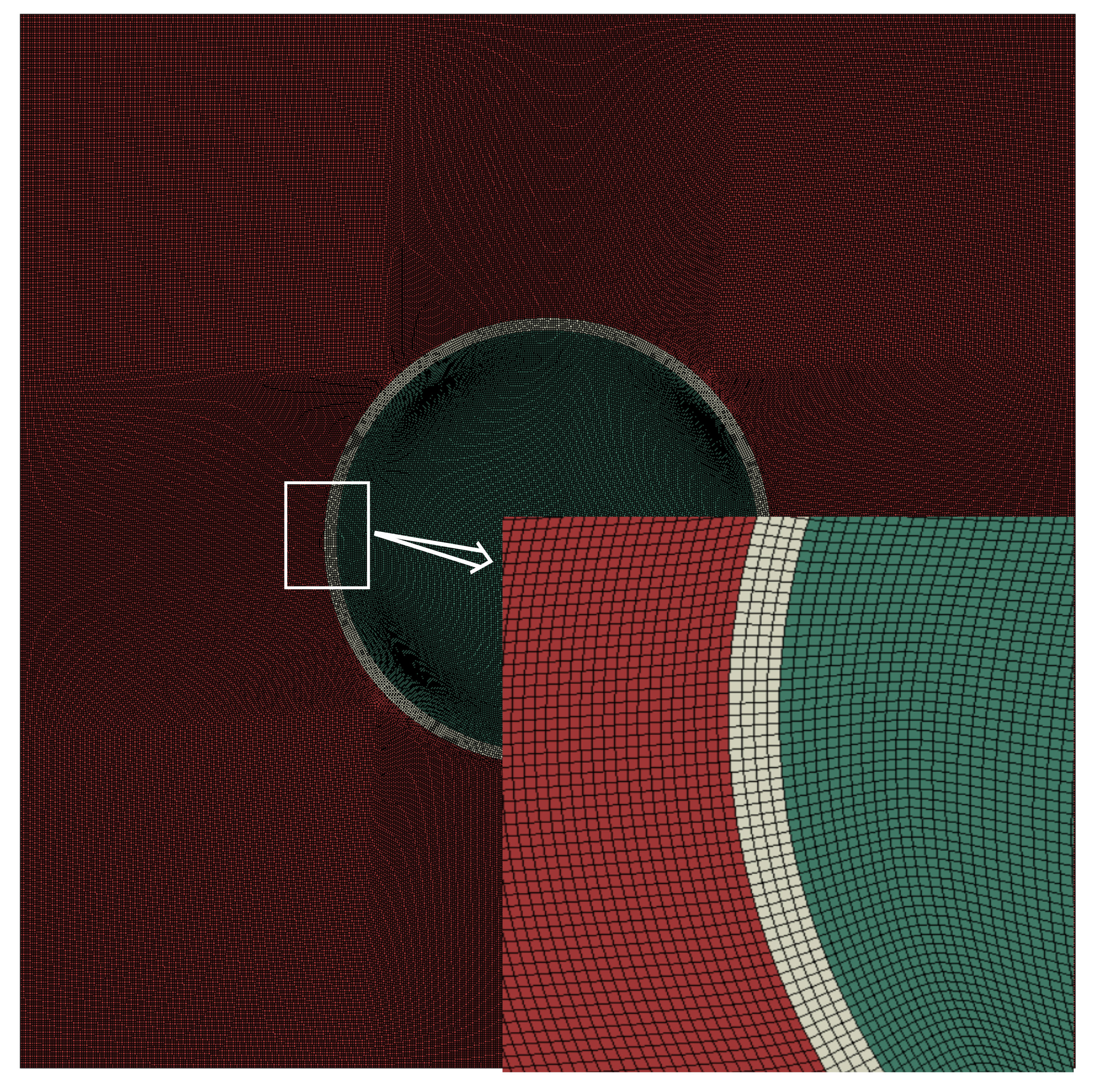
(a)

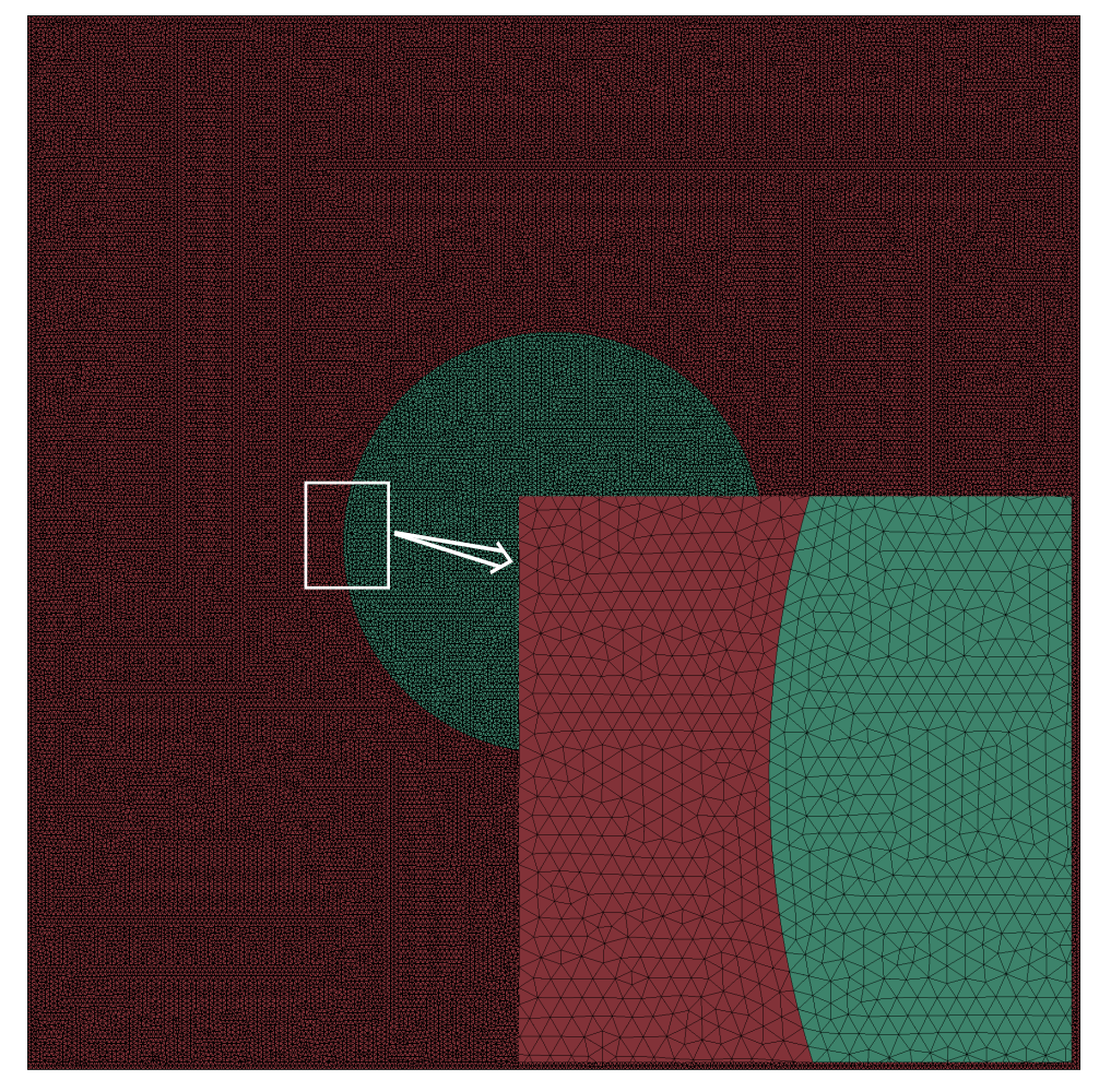
(b)

Figure 7: Finite element discretization for (a) phase-field fracture simulations, (b) cohesive zone model simulations.

Material properties relevant to the CZM and PFM simulations are provided in Table 2 and Table 3, respectively. It is worth noting that inclusions generally have significantly higher mechanical strength than other constituents, and it is a well-known phenomenon that cracks in many engineering materials do not propagate into the inclusions. Consequently, inclusion’s damage properties are not explicitly specified in CZM simulations. To account for this inherent behavior, the failure strength of inclusions is deliberately set to a much higher level than that of the other phases in the PFM simulations.

Table 2: Material properties for CZM simulations. The properties of inclusion and matrix including Young’s modulus, Poisson’s ratio, and the $\eta$ parameter, are derived from [88]. The elastic stiffness of CIEs is referenced from [89]. The input parameters for the TSLs in relation to CIEs are obtained from [82].

Parameter	Inclusion	Matrix	CIE- Interface	CIE- Matrix	CIE- Inclusion
Elastic Modulus, $E$ (GPa)	72	28	-	-	-
Poisson’s ratio, $\nu$	0.16	0.2	-	-	-
Elastic Stiffness, $K_{n}$ (MPa/mm)	-	-	$10^{6}$	$10^{6}$	$10^{6}$
Maximum normal stress, $\sigma_{n}^{0}$ (MPa)	-	-	2.4	4	-
Maximum shear stress, $\sigma_{s}^{0}$ (MPa)	-	-	10	30	-
Normal mode fracture energy, $G_{I}$ (N/mm)	-	-	0.02	0.06	-
Shear mode fracture energy, $G_{II}$ (N/mm)	-	-	0.4	1.2	-
B-K criterion material parameter, $\eta$	-	-	1.2	1.2	-

Table 3: Material properties for phase-field simulations. The Young’s modulus of the interface zone is obtained from [76].

Phase	Young’s modulus $E$ (GPa)	Poisson’s ratio $\nu$	Fracture energy $G_{c}$ (N/mm)	Failure strength $\sigma_{u}$ (MPa)
Inclusion	72	0.16	0.2	20
Matrix	28	0.2	0.06	4
Interface	21.9	0.2	0.02	2.4

The staggered scheme suggested by Gergely is used to solve the system of non-linear equations. Using the open-source ABAQUS codes from Gergely as mentioned in [90], the CPFM approach is integrated into the ABAQUS UEL subroutine by modifying the equations outlined in Table 5.

In simulations employing the CPFM, considering Equation 24, the softening zone is characterized by the utilization of the parameter sets

$$a_{2}=1.3868,\quad a_{3}=0.6567,$$ (36)

where these sets of parameters yield the Cornelissen’s softening relationship related [91] to concrete materials.

4 Results

In the present study, a benchmark model featuring a 2D specimen with a single circular inclusion is selected to assess the performance of four fracture modeling schemes applied to particulate composite materials, like concrete, at smaller length scales. The analysis primarily focuses on assessing numerical efficiency within these modeling frameworks. Following this initial study and maintaining consistent boundary conditions and material properties, the benchmark model is extended to consider more complex states characterized by multiple randomly distributed inclusions. To demonstrate the feasibility of extending the fracture models into 3D, a three-dimensional benchmark model, employing the most efficient fracture scheme, is also incorporated in this study.

When conducting phase-field simulations, a staggered solution scheme is used. This technique is characterized by a sequential approach to solving variables in which the phase-field and displacement fields are not solved simultaneously, which is in contrast to the methodology of a monolithic solver. Given the integration of a phase-field gradient parameter in the PFM formulations, it is imperative to carefully select the time step increment. An increment that is too large can produce incorrect results in terms of the simulated fracture paths and reaction forces. In this study a step time increment of $5\times 10^{-03}$s is utilized in the phase-field simulations. For CZM simulations, the Abaqus explicit solver is employed. This solver is selected due to the highly non-linear nature of the finite element model, which arises from the incorporation of zero-thickness cohesive interface elements within the initial mesh file, leading to observable convergence problems when utilizing standard solver. To mitigate dynamic effects in CZM simulations, one way is to opt for a minimal step time increment in the finite element simulation. In this study, a step time increment of $5\times 10^{-5}$s is adopted for CZM simulations. Monitoring the history of kinetic and total energy in the simulations reveals that, with this chosen step time increment, the kinetic energy remains less than 5% of the total energy. This observation indicates that dynamic effects are effectively mitigated in the finite element simulations through the adopted step time increment. Additionally, in this study, the reaction force-displacement curves are derived by averaging the reaction forces of the nodes situated along the left-hand side vertical edge, unless otherwise specified.

4.1 $l_{c}$ sensitivity analysis

As illustrated in Equation 15, the phase-field fracture model is formulated as an energy minimization problem. Through the minimization of the total energy functional (see Equation 14), the displacement $\bm{u}$ and phase-field fracture parameters $\phi$ are determined. Consequently, unlike the CZM, the simulated fracture paths in the phase-field model are no longer dependent on the mesh configuration. The width of the fracture zone in PFM models is regulated by the length scale parameter $l_{c}$. Nevertheless, when addressing small-scale fracture simulations, particularly in multiphase materials, pronounced limitations can be observed in the implementation of the SPFM approach. Subsequent sections will provide a detailed examination of these limitations and propose remedies to overcome the associated challenges.

4.1.1 Standard phase-field fracture

In the present analysis, a sensitivity study focusing on the length scale parameter $l_{c}$ is performed using a 2D benchmark model within the framework of the AT2 standard phase-field fracture model. In this study, all parameters are held constant, with the single variable $l_{c}$ systematically increased in the range from 0.3 mm to 0.6 mm. Figure 8 displays the simulated fracture paths for various $l_{c}$ values. For these simulations, a mesh size of 0.1 mm was selected for finite element analyses. From analyzing of the reaction force-displacement curves shown in Figure 9, two distinct features are evident as shown in [92]:

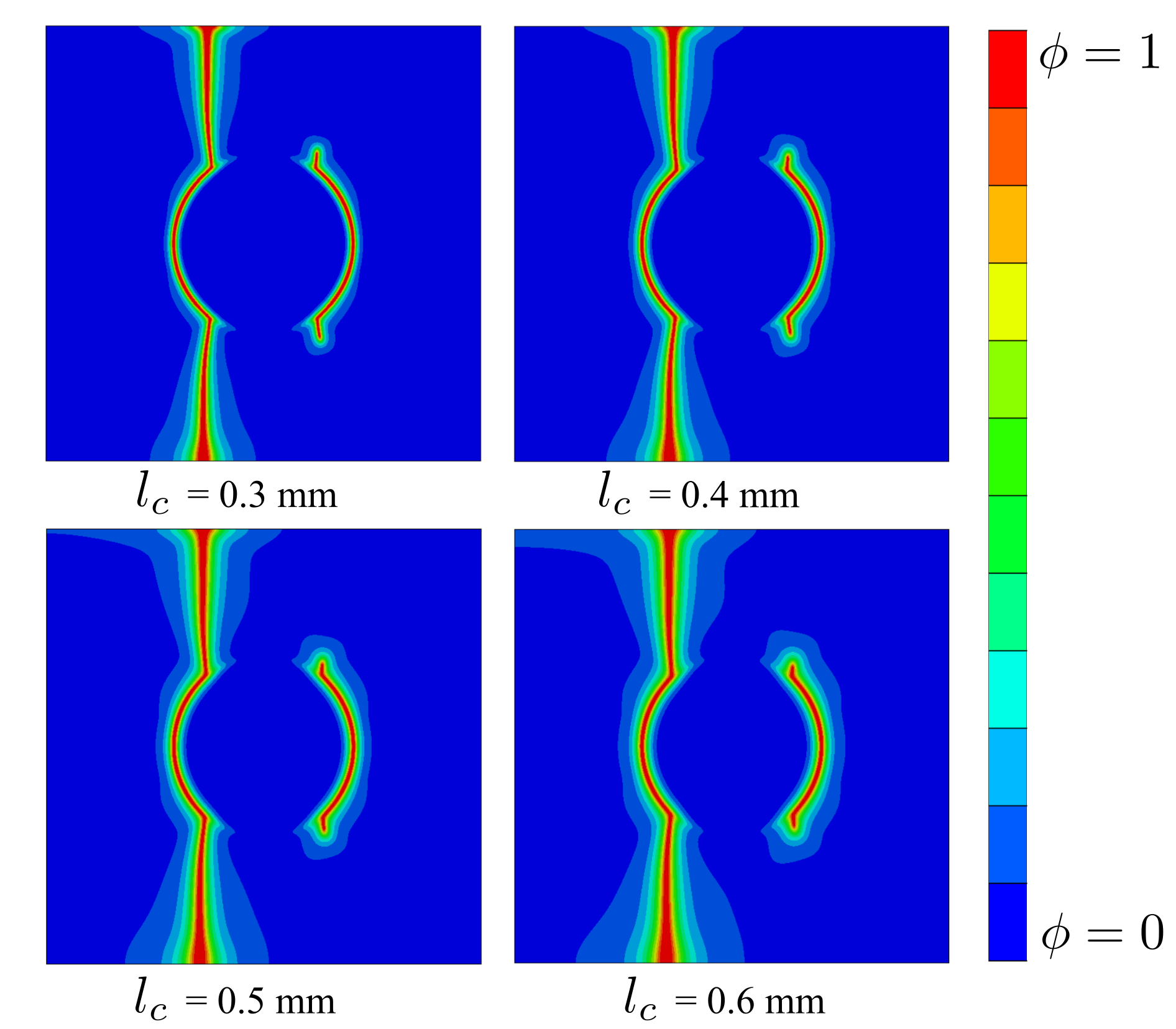
Figure 8: Fracture paths in the 2D single inclusion model have been simulated under tensile loading conditions. Here, $\phi$ denotes the phase-field fracture parameter, with $\phi=0$ indicating no damage, and $\phi=1$ illustrating a complete fracture.

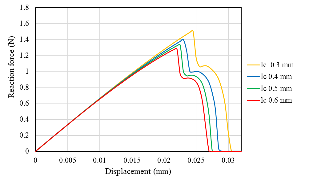
Figure 9: Sensitivity analysis of the parameter $l_{c}$ conducted using the AT2 standard phase-field fracture model.

• The standard phase-field fracture model shows sensitivity to $l_{c}$. A notable observation is that an increase in the value of $l_{c}$ is accompanied by a decrease in the peak reaction force.

• For a range of $l_{c}$ values, there is a notable sharp decrease in reaction force accompanied by a slight increase in displacement that occurs after the peak reaction force is reached.

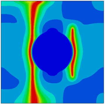
Figure 30: Fracture paths in the 2D single inclusion model have been simulated under tensile test conditions. In this simulation the mesh size is 0.15 mm.

Figure 30 depicts an AT2 standard phase-field simulation conducted on the benchmark model, which is discretized with a mesh size of 0.15 mm. It’s important to note that all simulations in this study utilize the same mesh size of 0.15 mm. However, as clearly illustrated by Figure 30, this particular mesh size results in unsatisfactory outcomes, especially in terms of the simulated fracture paths when SPFM approach is used. A comparison between Figure 8 and Figure 30 reveals a significant enhancement in the simulation outcomes when the mesh size is reduced from 0.15 mm to 0.1 mm. Nevertheless, such enhancement comes at the expense of a substantial increase in computational cost. The unsatisfactory results with the coarse mesh originates from the fact that in standard phase-field simulations, the crack geometric function $\alpha(\phi=1)$ either never reaches zero (as in the AT2 model) or reaches zero (in the AT1 model) at a higher magnitude of $x/l_{c}$ compared to the cohesive phase-field fracture model, as shown in Figure 2. Therefore, to exclude the diffusion of the gradient term of the phase field parameter $\nabla_{\!\underaccent{\tilde}{x}}\phi$ over different regions of the benchmark model, it is essential to choose a very fine mesh, which requires a corresponding reduction of the parameter $l_{c}$.

From the previous findings, it should be mentioned that $l_{c}$ cannot be considered only as a numerical parameter in the context of SPFM approach. The use of a simplified analytical solution has clarified the relationship between the $l_{c}$ parameter and the strength of the material [78, 93, 7]. In addition, $l_{c}$ was experimentally determined through the measurement of critical stress in uniformly stretched samples [92]. This inherent property of the SPFM model limits its application to simulations at smaller length scales, such as mesoscale or microscale simulations. With this approach, users are limited to a specific length scale parameter that is intrinsically linked to material properties and cannot intentionally change it. This limitation can lead to inaccurate results for simulations at small scales, as a larger value of $l_{c}$ can lead to boundary effects.

4.1.2 Cohesive phase-field fracture

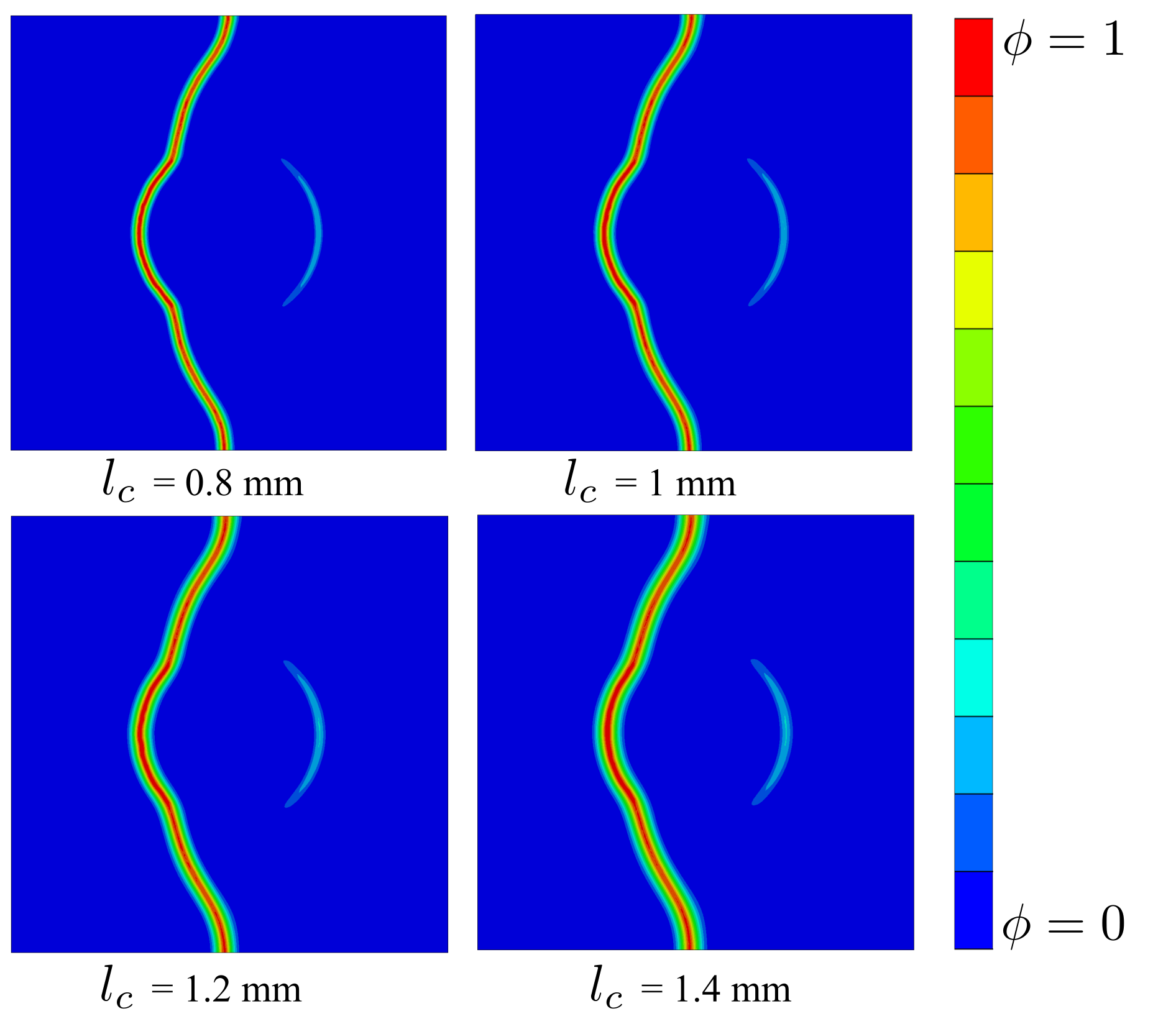
Figure 10: Fracture paths in the 2D single inclusion model have been simulated under tensile test conditions. Here, $\phi$ denotes the phase-field fracture parameter, with $\phi=0$ indicating no damage, and $\phi=1$ illustrating a complete fracture.

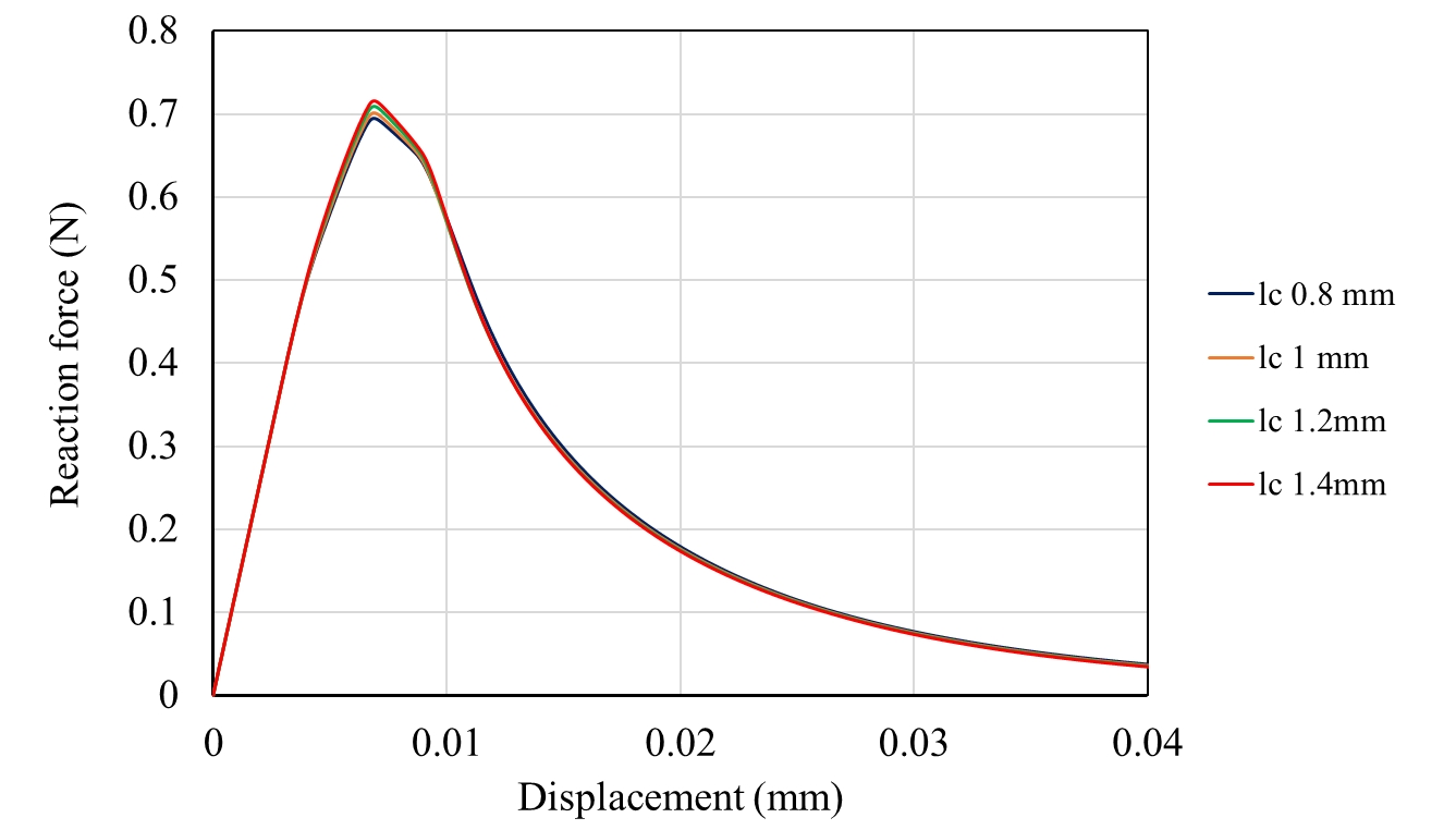
Figure 11: Sensitivity analysis of the parameter $l_{c}$ conducted using the cohesive phase-field fracture model.

In the present investigation, a sensitivity analysis focusing on the $l_{c}$ parameter is conducted, utilizing a CPFM approach on a benchmark 2D model. Analogous to the SPFM methodology, all model parameters are held constant with the exception of the $l_{c}$ parameter. The value of this specific parameter is systematically varied within the range of 0.8 mm to 1.4 mm for the purpose of examining its impact on the predicted fracture paths and reaction force as function of displacement.

Figure 10 depicts the simulated fracture paths of the benchmark 2D model utilizing the CPFM approach. It is observable that unique fracture paths are evident with variations in the value of $l_{c}$. Moreover, contrary to the SPFM approach by employing the mesh size of 0.15 mm, the damage zone is observed to be localized, not diffusing throughout the entire specimen. As shown in [19] and also evident from Figure 11, two principal conclusions can be deduced:

• The CPFM approach demonstrates insensitivity with respect to the length scale parameter. Variations in the value of $l_{c}$ yield negligible effects on the reaction force-displacement relationship. This observation is indicative of the proposed modifications in the formulations, which have effectively transformed $l_{c}$ from a material parameter to a numeric one.

• Cohesive behavior is observed in the reaction force-displacement diagrams. There is no abrupt decrease in reaction force after the onset of the softening zone; instead, a gradual decrease in reaction force after the onset of damage is observed when additional displacement is applied. This property allows for the simulation of semi-brittle materials, such as concrete.

This observation leads to a pivotal conclusion: when aiming to simulate at smaller length-scales, such as mesoscale or microscale, one is not constrained by the $l_{c}$ parameter any longer. Consequently, the CPFM approach emerges as a superior choice for conducting fracture simulations of multiphase materials at smaller length-scales.

4.1.3 Hybrid model

When the thickness of the interface zone in a composite material is considerably smaller than that of the other phases, the hybrid modeling technique emerges as the most suitable approach. This is particularly evident in real-world scenarios involving the microstructure of materials such as concrete at the meso or microscale. An illustrative example can be seen in the Scanning Electron Microscope (SEM) image of concrete’s microstructure (see Figure 12). As explained by [94], the interface zone in concrete, with a thickness ranging between 20-100 $\mu m$, is characterized by markedly reduced mechanical properties. Consequently, under loading conditions, damage typically initiates in this weaker interface zone before progressing into the other phases. This observation underlines the importance of the hybrid model for accurately capturing the mechanical behavior of such materials.

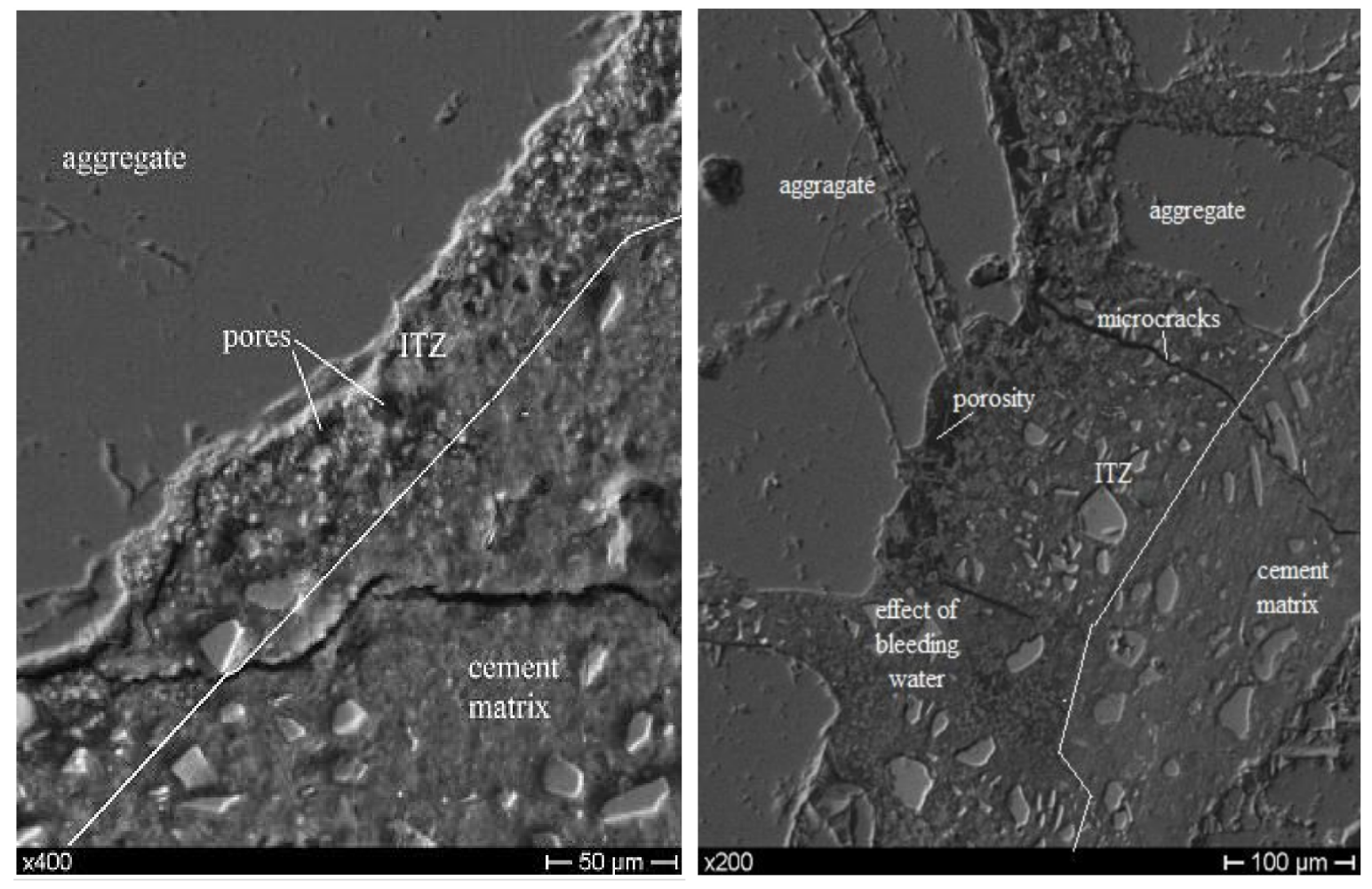
Figure 12: SEM imaging of interface zone in concrete materials [94]. The interface zone in concrete materials has a thickness between 20-100 µm, which, compared to other phases, is very small. Direct realization of this influential phase in FE simulations would be very challenging due to the required very fine element size. Hence, a hybrid model in which the interface debonding is modeled using zero-thickness cohesive interface elements, combined with a phase-field fracture approach for matrix cracking, could be a solution to this problem.

To develop a reliable numerical model for materials with very thin interfaces, it is imperative to incorporate the weak interface zone into the numerical simulations. However, given the comparative scale of the actual size of other phases, the interface zone’s thickness is quite small, and its direct inclusion poses significant challenges in numerical simulations. Due to the interface zone’s minimal thickness, extremely fine elements are required for its discretization. This fine meshing would yield a substantial number of elements, consequently leading to a pronounced escalation in computational cost. Addressing this challenge can be achieved through the implementation of CIEs within the interface zone. In the hybrid model in this work, the CPFM approach is employed for both the matrix and inclusion. Furthermore, in the hybrid model, the interface zone is represented by generating CIEs at the boundary between the inclusion and matrix, with the TSL properties of the ITZ being assigned to these interface elements. Besides, interested readers are referred to the research in [95, 96] for modeling cracking in polycrystalline materials by combining standard phase-field damage models with CZM. In the Figure 13, the fracture paths obtained from hybrid model are shown. It is obvious that the contour plots of the damage are localized in a specific region and do not diffuse throughout the entire model. Also, a slight increase in the width of the diffused crack is observable, which is accompanied by an increase in the value of $l_{c}$. Moreover, a $l_{c}$ sensitivity analysis is performed using the hybrid formulation on a 2D benchmark model. The results of the $l_{c}$ analysis are shown in Figure 14. Analogous to the results of the CPFM method, the hybrid model is insensitive to $l_{c}$ and exhibits cohesive properties, which can be observed in the reaction force-displacement curves.

The results obtained suggest that the hybrid model serves as an appropriate option for conducting small-scale simulations in multiphase materials, particularly when the interphase thickness is significantly smaller than that of the other phases.

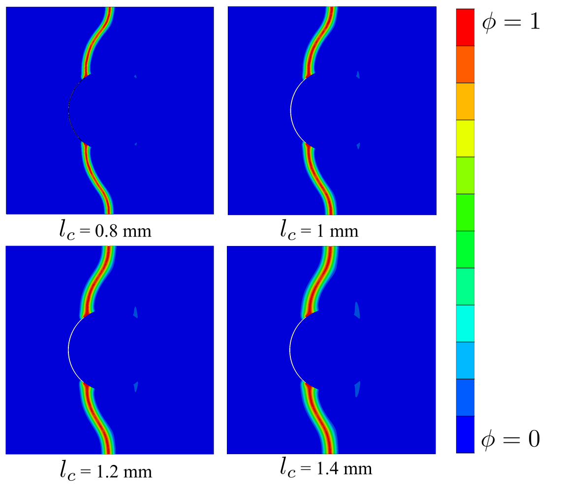
Figure 13: Fracture paths in the 2D single inclusion model have been simulated under tensile test conditions. CZM formulation is utilized in the interface zone and CPFM approach is utilized within mortar matrix and inclusion. Here, $\phi$ denotes the phase-field fracture parameter, with $\phi=0$ indicating no damage, and $\phi=1$ illustrating a complete fracture.

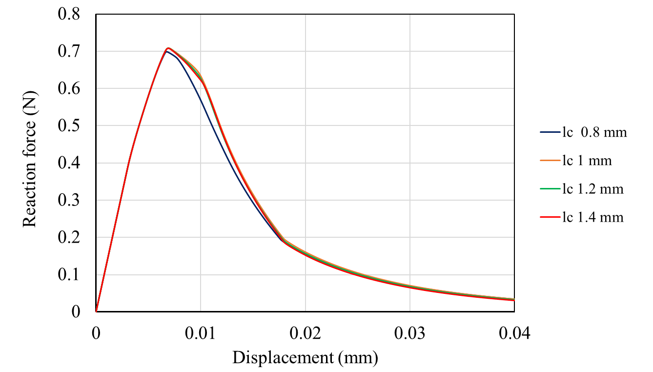
Figure 14: Sensitivity analysis of the parameter $l_{c}$ conducted using the hybrid model, i.e. a combination of cohesive phase-field fracture and cohesive zone models.

4.2 Evaluating Numerical Efficiency

In this section, the introduced methods to simulate fracture in multiphase materials at small length scales are compared. The comparison is carried out in terms of computational time and total number of iterations in a complete successful finite element simulation. It is worth mentioning that the SPFM is not compared with other methods. The reason for this exclusion stems from the observations in Section 4.1.1, where it was noted that for SPFM the $l_{c}$ depends on the material properties, limiting the selection of an appropriate size for $l_{c}$. Furthermore, due to the inherent formulation of SPFM, a significant reduction in mesh size is mandatory to achieve realistic simulations of multiphase materials in terms of fracture paths. However, this reduction in size would lead to a significant increase in computational cost. Considering that a mesh size of 0.15 mm is used for finite element simulations in this study, and the fact that SPFM with this mesh size gives unsatisfying results in terms of simulated fracture paths, this approach is removed from the comparison in order to maintain consistency.

Figure 15 shows the fracture paths simulated using the CZM, hybrid, and CPFM modeling approaches. Under the similar boundary conditions for the benchmark model, all three modeling methods yield fairly analogous fracture paths. Concerning the computational cost and the total number of iterations, the following key points can be made for each of the models:

• Cohesive Zone Model:
  In Cohesive Zone Modeling simulation, the nonlinear equation systems are solved using the ABAQUS/Explicit software. This choice is primarily due to the significant degree of nonlinearity introduced by the implementation of CIEs within the initial mesh file. To ensure quasi-static loading conditions, as recommended in studies such as [97] and [89], it becomes necessary to use a very small step time increment in FE simulations. This approach effectively mitigates dynamic effects. However, the trade-off is a substantial increase in computational cost due to the reduced step time increment. Utilizing a mesh size of 0.15 mm resulted in a total of 128,286 solid elements and 191,929 CIE elements in the CZM simulation for the 2D benchmark. This simulation necessitated three days, utilizing 5 CPUs of the type Intel(R) Xeon(R) Platinum 8280. Figure 16a shows a significant deviation in the simulated reaction force-displacement curve for the CZM model compared to the hybrid and CPFM models. Even in the elastic region, a deviation is observed. This observed behavior could be attributed to the need to calibrate numerous numerical parameters of the TSL before assigning them to the CIEs belonging to the different phases. The elastic stiffness parameter, $k_{n}$, is particularly important since it determines the stiffness of the connections between solid elements. Extremely low or high values of $k_{n}$ can lead to numerical problems. In this study, $k_{n}$ is determined to be $10^{6}$ MPa/mm. Attempting to improve the deviation in the slope of the elastic region by increasing the value of $k_{n}$ resulted in ill-conditioned simulation results. In summary, given the long simulation time, the tendency for numerical problems to arise primarily from the introduction of a large number of numerical parameters, and the complexity of constructing the CZM model from an initial FE mesh file, CZM does not prove to be an optimal approach for performing small-scale simulations of multiphase materials.

  

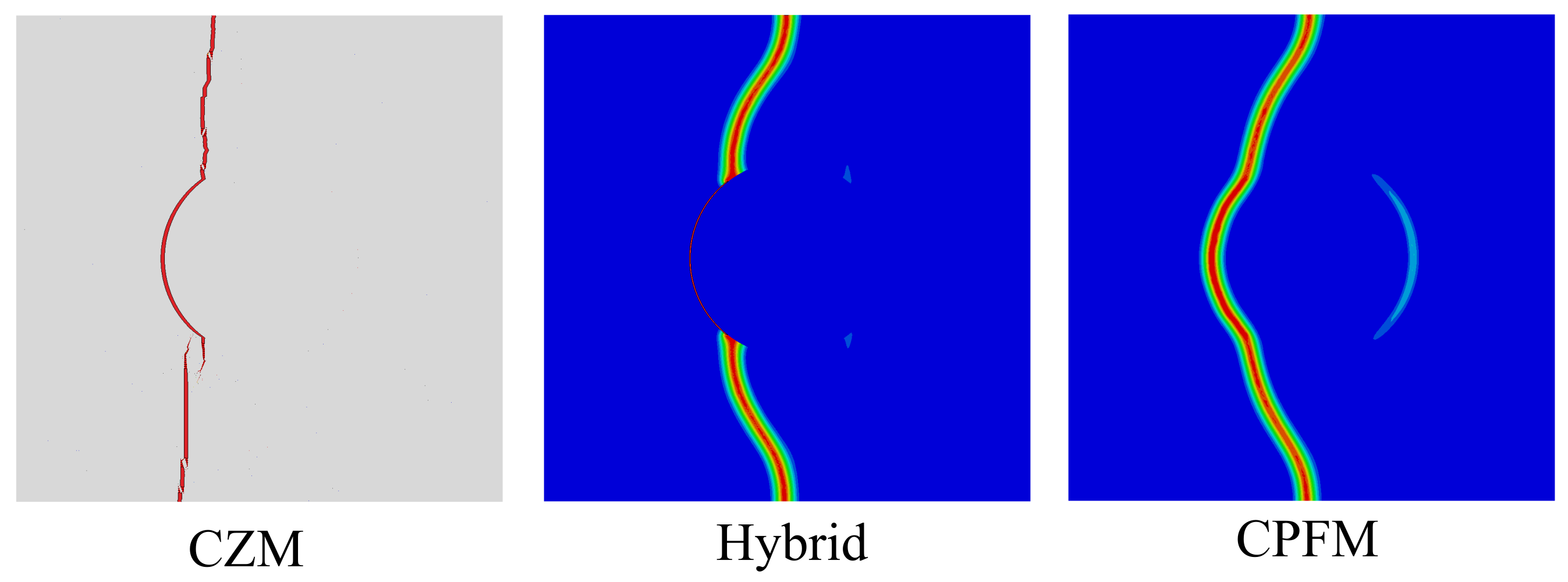
  Figure 15: Simulated fracture paths by implementing the Cohesive Zone Model (CZM), Cohesive Phase-Field Fracture (CPFM), and a hybrid approach within a two-dimensional single inclusion model, under the boundary conditions illustrated in Figure 6(a).

  

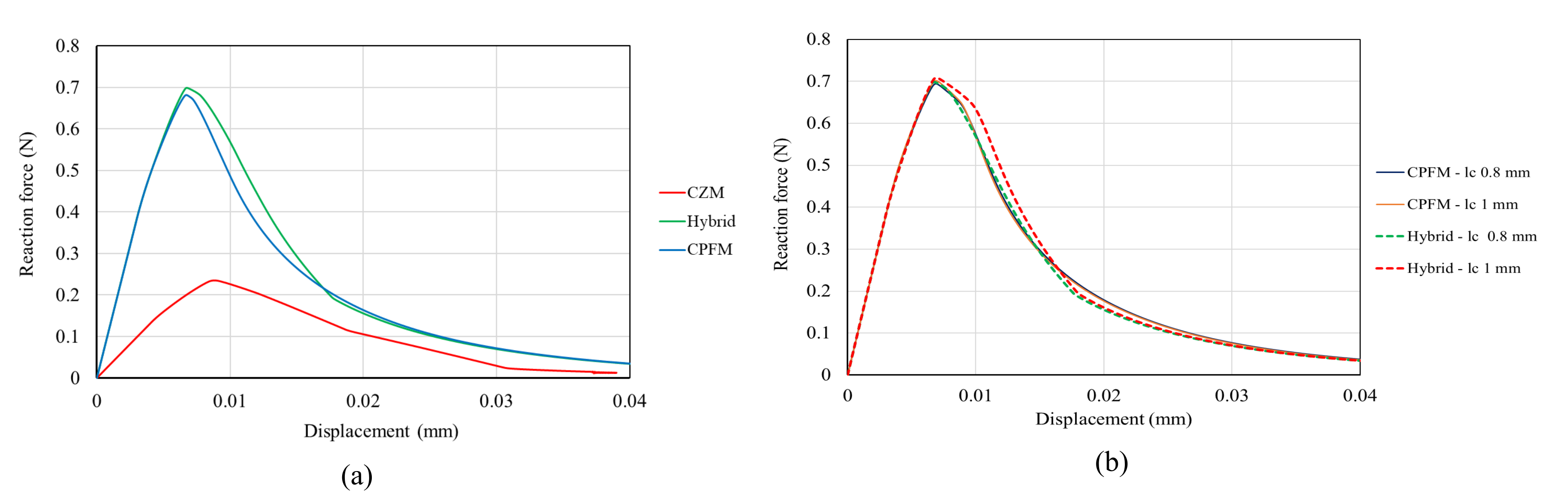
  Figure 16: A quantitative analysis is represented, featuring: (a) the reaction force-displacement curves acquired through finite element simulations of the two-dimensional single inclusion model, employing the CZM, CPFM, and the hybrid Approach; and (b) a comparative study of the $l_{c}$ sensitivity analysis, conducted utilizing both the hybrid and the CPFM fracture models.

• Hybrid Model:
  Section 4.1.3 explains that the hybrid model bears a strong resemblance to the microstructure of concrete, which is a significant advantage in structural health monitoring (SHM) of concrete structures. An important aspect of SHM is to optimize the placement of sensors to accurately monitor the structural health of infrastructures, such as bridges. This optimization can be achieved through mesoscale simulations of concrete materials within a FE2-type multiscale simulation framework. In these mesoscale finite element simulations, the initiation and progression of microcracks can be represented with high accuracy. This allows critical points in concrete structures, such as bridges, to be identified with high precision. Through the optimal placement of sensors, the propagation of cracks can be detected early and accurately. Nevertheless, the hybrid model is not free of certain limitations, which are described below:

  1. Model complexity:
     The hybrid model combines two distinct fracture models, integrating them within a single finite element framework. This integration necessitates additional effort, as it involves developing two sets of essential tools during the pre-processing steps. The first set pertains to the creation of codes for generating CIEs in the targeted area, following the intrinsic CZM approach. In this study, these codes are developed using Python. The second set focuses on the development of a user-element subroutine, which facilitates the implementation of the PFM fracture approach in commercial software such as Abaqus.

  2. Computational cost:
     The hybrid model effectively integrates both the CZM and the CPFM within a single finite element framework. This integration inevitably leads to an increase in the number of iterations required at each time step for the numerical solver to attain convergence. Consequently, the greater the number of iterations needed per step, the higher the computational cost becomes.

• Cohesive Phase-Field Model:
  The finite element analysis performed in this study has highlighted several characteristic features of CPFM fracture approach. Particularly noteworthy are its insensitivity to the length scale parameter and its more physical nature in terms of the parameters required for numerical simulations. The analysis presented in Figure 16a shows that the reaction force-displacement curve derived from the CPFM fracture approach closely matches that of the hybrid model. For further analysis, as shown in Figure 16b, the reaction force-displacement curve of the CPFM fracture approach is compared with that of the hybrid model for different values of the $\l_{c}$ parameter. The results highlight that the results of the CPFM model consistently converge with those of the hybrid model. This presents significant benefits, particularly for smaller-scale simulations of multiphase materials. Utilizing a simpler and less computationally intensive model for mesoscale simulations of multiphase materials, while still harnessing the advantages of the CPFM model, becomes feasible. Figure 17 provides a comparative analysis between the hybrid model and the CPFM fracture approach in terms of computational time for a successful simulation and the total number of iterations required. Notably, the CPFM approach is more computationally efficient than the hybrid model. The key findings from this study indicate that the CPFM fracture methodology emerges as the preferred technique for fracture simulations, especially for multiphase materials at smaller scales, provided that the interphase thickness is relatively substantial in comparison to the other constituent phases. It is worth mentioning that in cases where the interface thickness is very small, such as in the ITZ zone of concrete materials, it is possible to artificially increase interface thickness and scale its material properties accordingly. In other words, CPFM can be adapted to become an interface width-insensitive fracture approach (refer to [61])

Given the advantages of the CPFM approach, it proves to be a well-suited modelling technique, also in view of microstructural optimization in terms of fracture properties and for the generation of data-driven surrogate models for the prediction of mechanical properties and fracture paths. This modeling approach facilitates the efficient execution of extensive simulations on complex heterogeneous microstructures and offers the advantage of low computational costs. Consequently, it enables a larger number of simulations to be carried out within a relatively short time frame. Hence, in Section 4.3 the ability of the CPFM approach to deal with more complex state and its adaptability in challenging modeling scenarios is demonstrated. Subsequently, the potential of the CPFM approach for microstructural optimization is discussed in Section 4.4. A crucial aspect of the CPFM approach is the identifiable nature of the constituent elements of the interphase zone. This property significantly improves the feasibility of microstructure optimization using methods such as the inverse finite element method or voxel-based finite element approaches. However, it should be noted that the use of the hybrid model for these tasks becomes more difficult when the interface zone is very thin. This complexity arises from the need for complicated algorithms to identify the interface zone and the challenge of incorporating the influence of this zone into the microstructural optimization. It’s noteworthy that there are advanced versions of the CZM, such as the finite thickness cohesive zone modeling technique, which can be incorporated into hybrid models. This particular technique is adept at approximating thin interface regions, facilitating a smooth transition between the interface region and other phases. However, its applicability may be limited in scenarios where the physical thickness of the interface region is relatively small. In such instances, employing this technique might not be feasible as the approximated interface thickness could be larger than the actual one. This limitation becomes particularly challenging in situations characterized by a high density of inclusions. Under these circumstances, scaling material properties becomes an essential step.

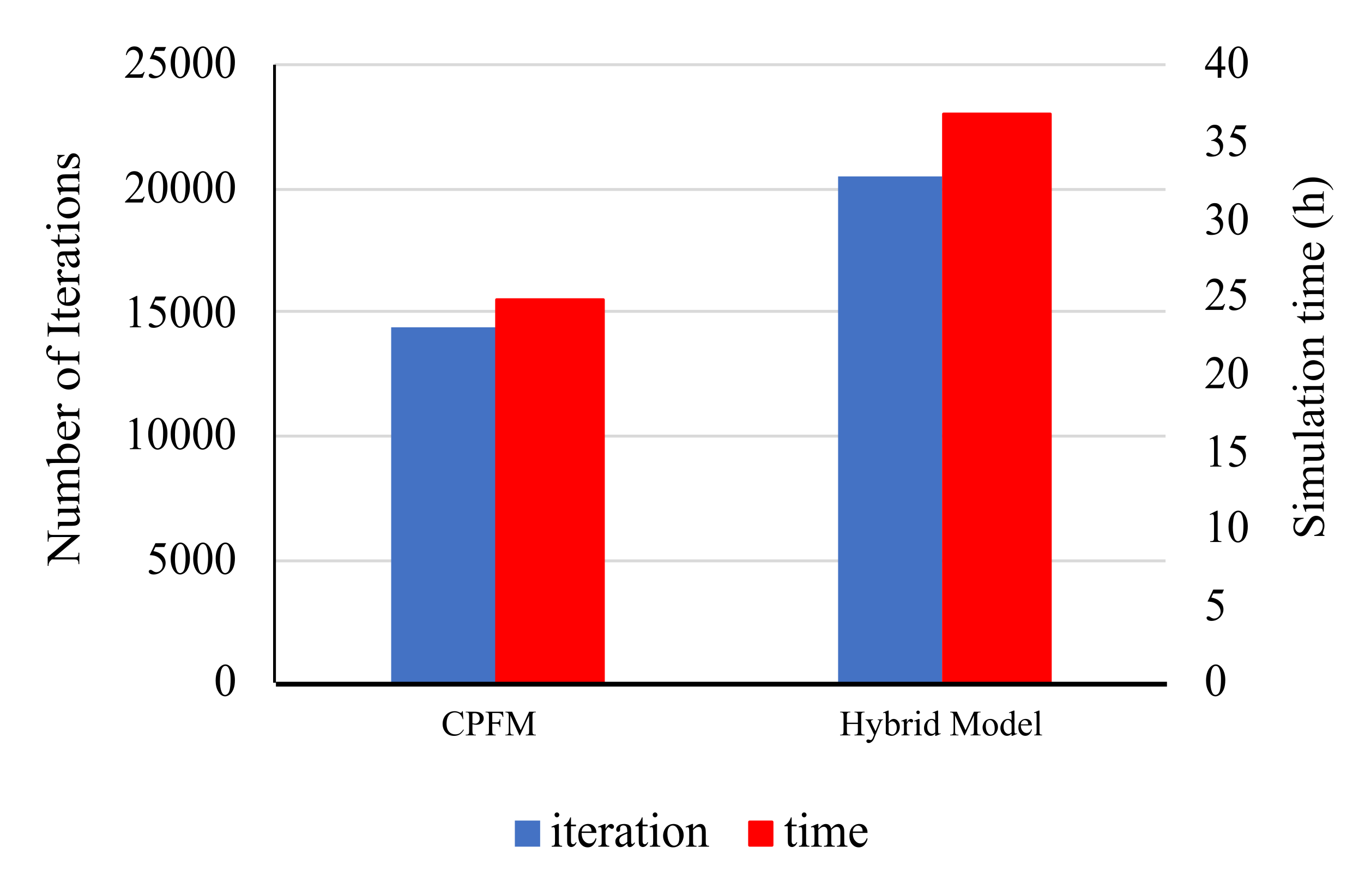
Figure 17: A comparative study focused on the numerical efficiency between the CPFM and the hybrid model.

4.3 Dimensional progression

In this section, the expansion of the CPFM approach to encompass more complex conditions is explored through the presentation of various finite element simulations.

4.3.1 Complex 2D Simulations

The simulated fracture paths in Figure 18 shows 2D models characterized by a stochastic distribution of inclusions. These inclusions account for 20% of the total volume fraction, with each inclusion comprising a 0.5 mm thick interphase layer. It is evident that finite element simulations are able to successfully reproduce complete fracture paths in models with multiple inclusions. Figure 19 shows a comparative analysis of the reaction force-displacement curves obtained from each model.

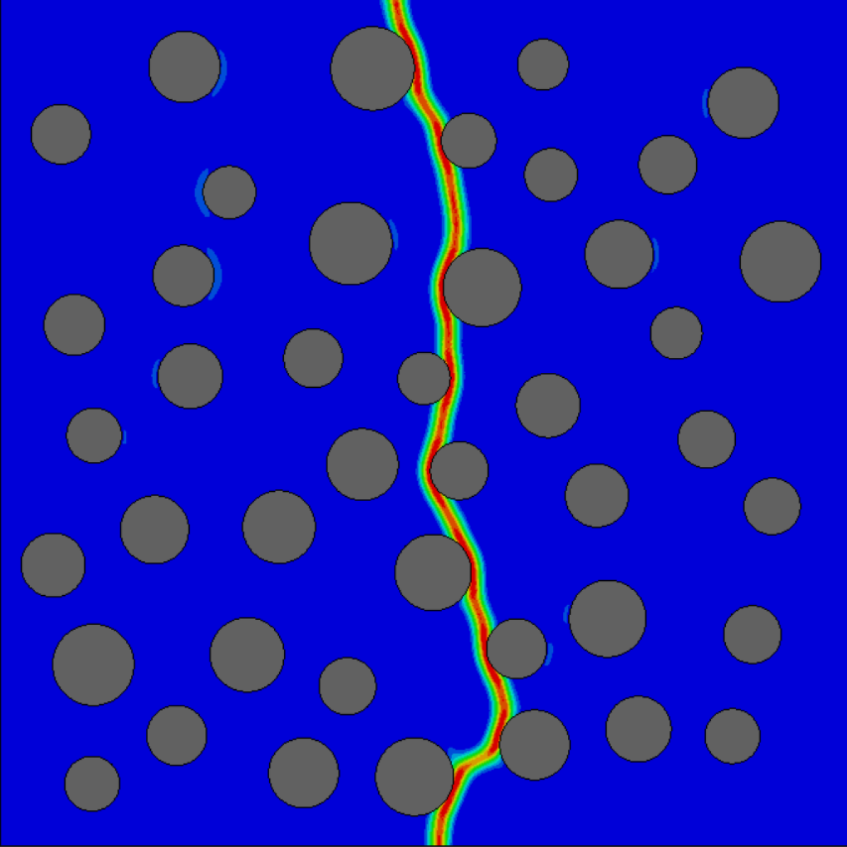
(a) Circular inclusions

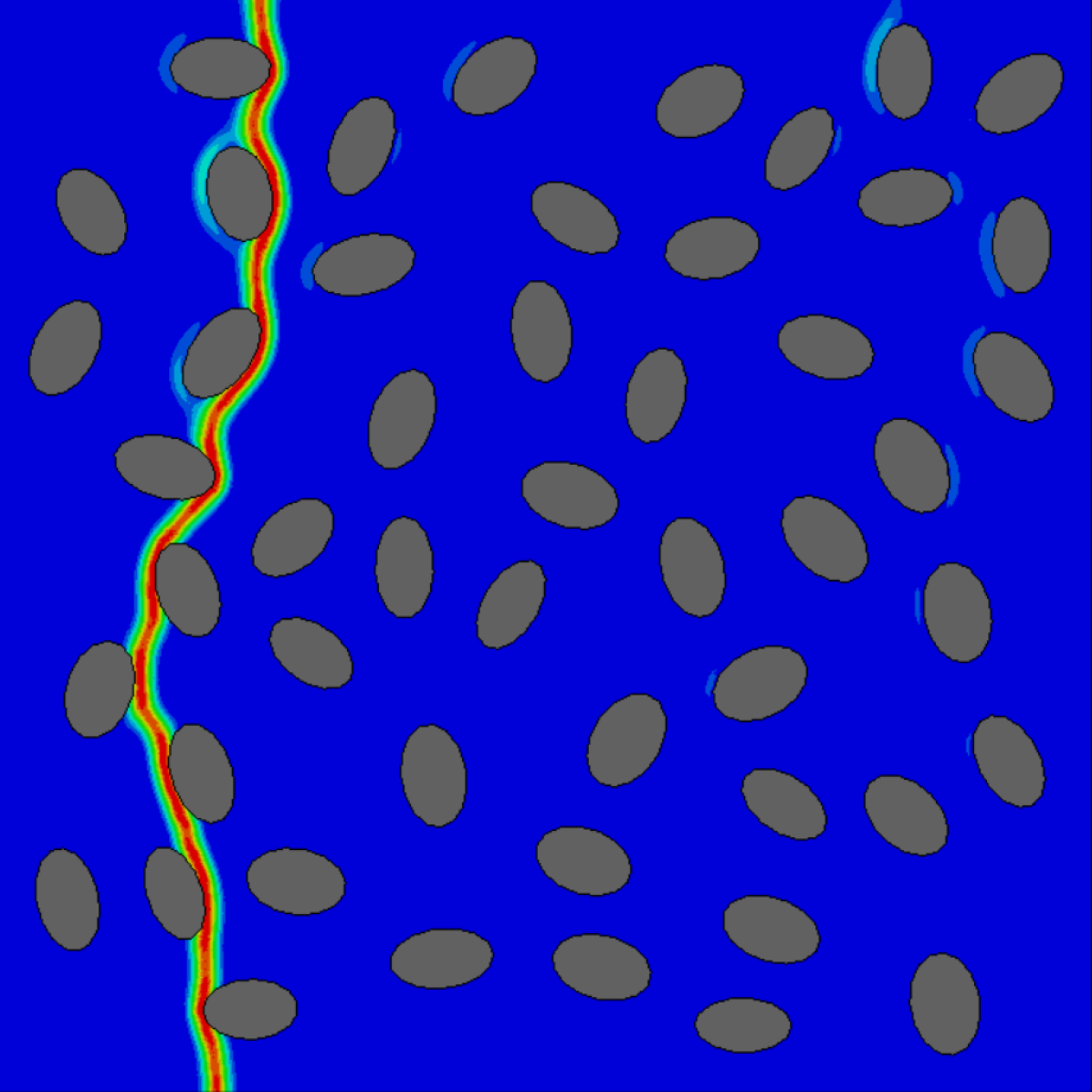
(b) Elliptical inclusions

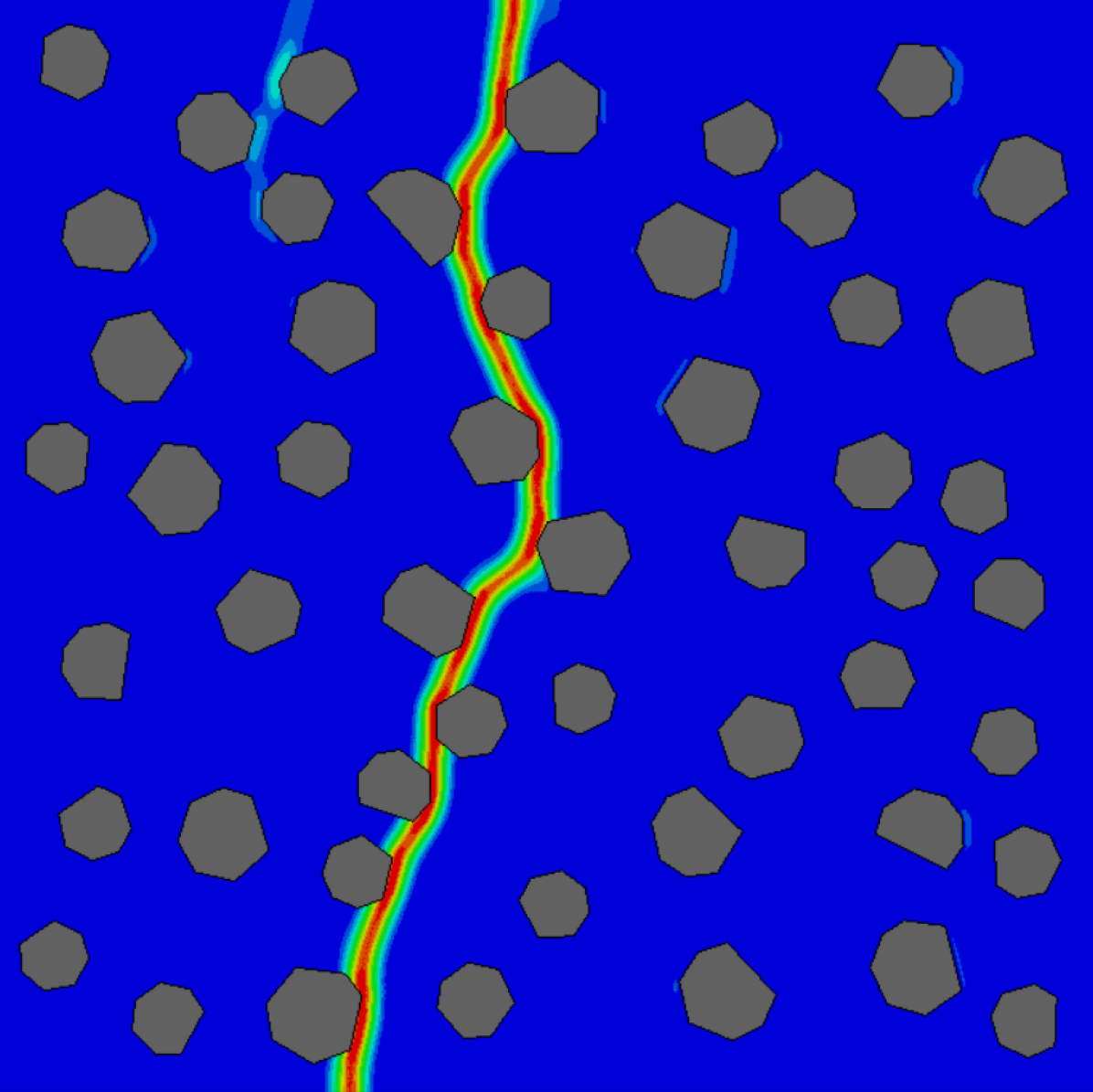
(c) Polyhedron inclusions

Figure 18: The study investigates fracture paths in complex models featuring multiple inclusions with interface regions. The model is 50 mm $\times$ 50 mm and the sizes of the inclusions vary between 6 mm and 8 mm. For these simulations, the CPFM technique is employed. The specific boundary conditions applied in the finite element analysis are illustrated in Figure 6(b).

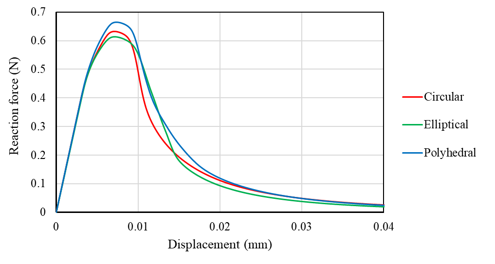
Figure 19: Reaction force-displacement curve from finite element simulations showcasing models with varied inclusion shapes and random spatial distribution of inclusions.

4.3.2 3D simulations

In this section, the capability of the CPFM fracture approach in simulating 3D boundary value problems for multiphase materials is demonstrated. A 3D model with a single inclusion, which has boundary conditions analogous to the 2D model, is chosen to represent the initiation and propagation of cracks. The dimensions and imposed boundary conditions are depicted in Figure 20(a). In Figure 20(b), a cross-section of half the model along the x-axis is shown to illustrate the three distinct phases.

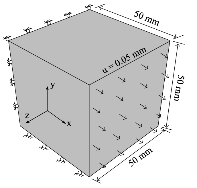
(a)

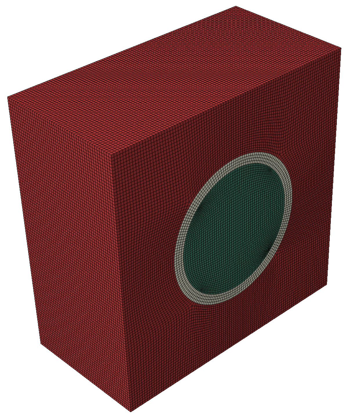
(b)

Figure 20: (a) Specified dimensions and boundary conditions are on the 3D specimen. (b) The 3D specimen incorporates a spherical inclusion surrounded by an interface region. To depict the phases, the model is halved in the x direction.

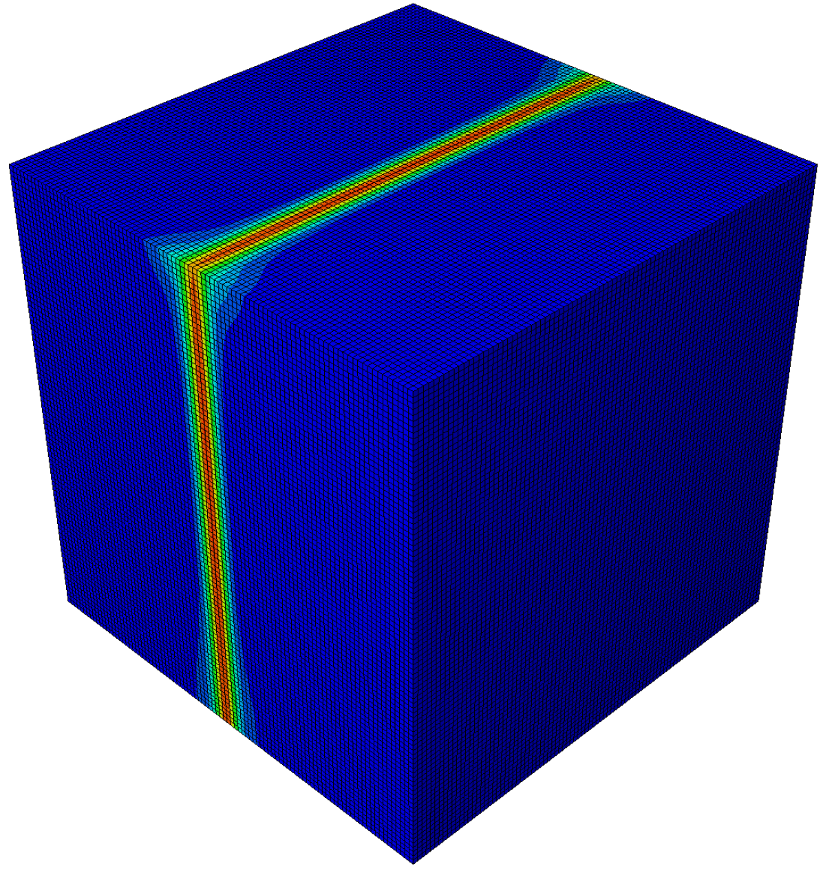
(a)

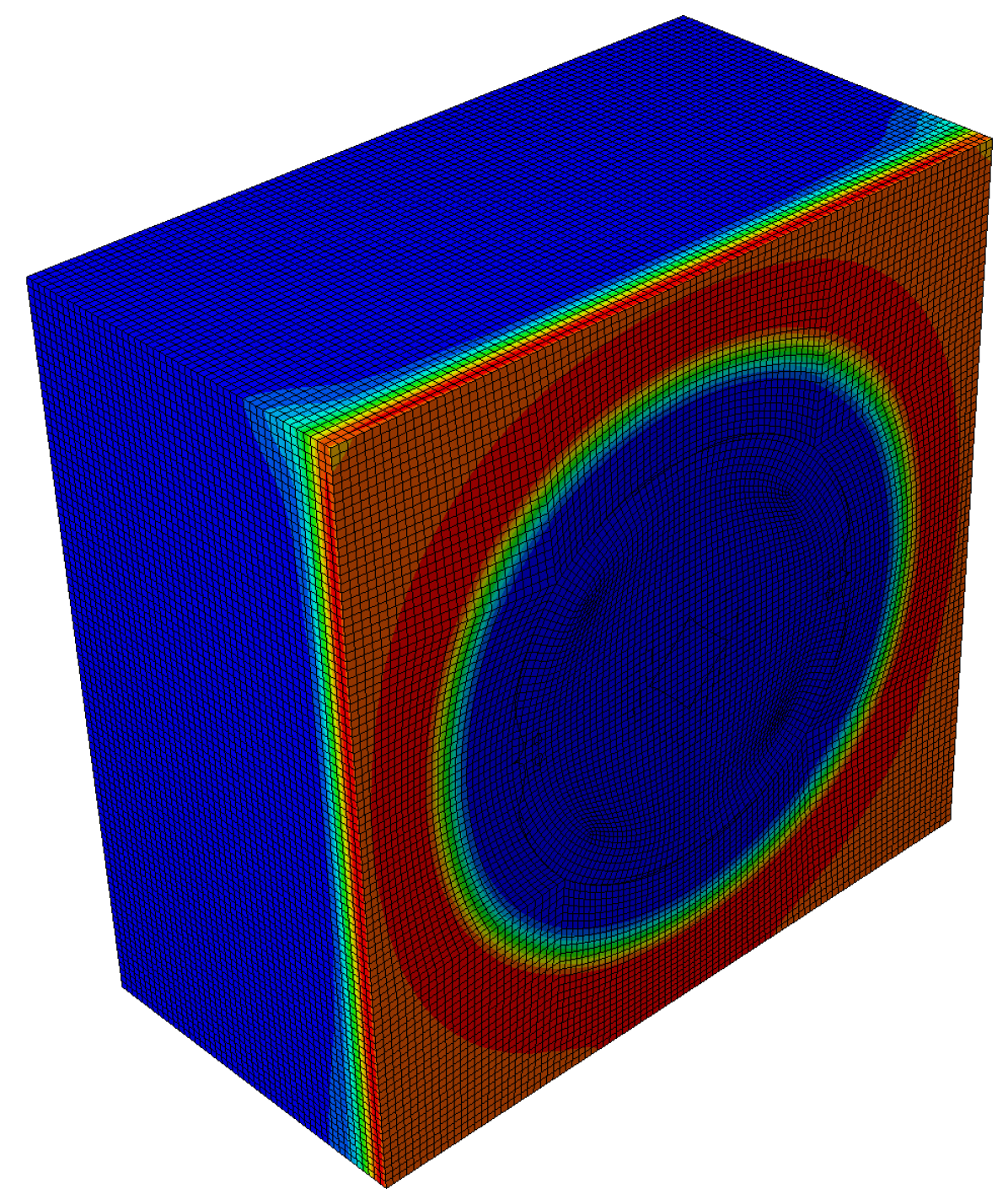
(b)

Figure 21: Fracture of a single 3D inclusion under the boundary condition shown in Figure 20(a). The images are extracted at the end of the simulation time.

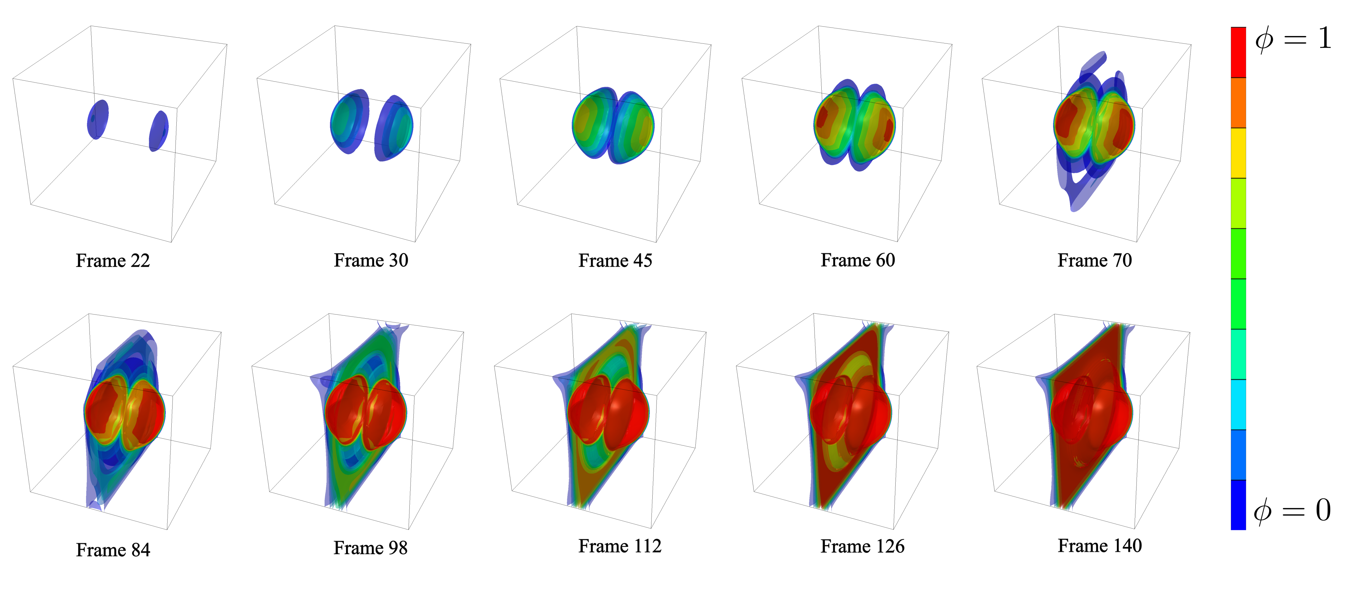
Figure 22: Initiation and propagation of fracture are modeled within a 3D single inclusion model. The cohesive phase-field fracture approach is utilized for the numerical simulation, which comprises a total of 140 frames.

Figure 21 illustrates the simulation outcomes using the CPFM approach for the 3D problem. Areas colored in blue indicate no damage ($\phi=0$), whereas the red regions signify damaged areas with $\phi>0.95$. The isosurface representation of the damage phase-field, showcasing the initiation and progression of the crack, is provided in Figure 22. As discerned from Figure 22, damage initiation occurs within the interface zone and subsequently propagates through the matrix.

Figure 23 clearly demonstrates the CPFM’s insensitivity to variations in $l_{c}$ in 3D simulations. Notably, changes in $l_{c}$ result in slight changes in force-displacement curves.

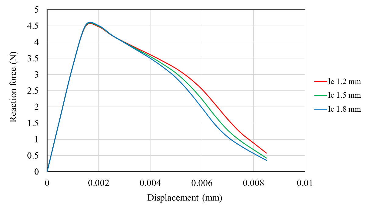
Figure 23: $l_{c}$ sensitivity analysis conducted on 3D single inclusion specimen using the cohesive phase-field fracture approach.

4.4 Microstructural Optimization Pathway

In this section, a comprehensive analysis is carried out to illustrate the combined influence of interface mechanical characteristics and geometric attributes of inclusions on the fracture properties of particulate composite materials. It is shown that the spatial distribution of inclusions has an influence on the fracture properties of multiphase materials. For further information, interested readers are referred to [98]. The aim of this study is to highlight not only the importance of the spatial distribution of inclusions but also the corresponding interface properties in the design optimization of composites, a factor that is often overlooked in many publications. To this end, the effects of the spatial distribution of the inclusions and interface mechanical properties are analyzed individually.

4.4.1 Impact of inclusion spatial distribution

The influence of the spatial distribution of the inclusions is investigated by examining four unique microstructures with ellipsoid aggregate particles, as depicted in Figure 24. Each of the models under study comprises three phases: matrix, inclusion, and interface zone. All the analyzed microstructures maintain the same volume fraction for both the inclusion and interface and are discretized by using a uniform mesh size of 0.15 mm. The boundary conditions for the finite element analysis are provided in Figure 6(b).

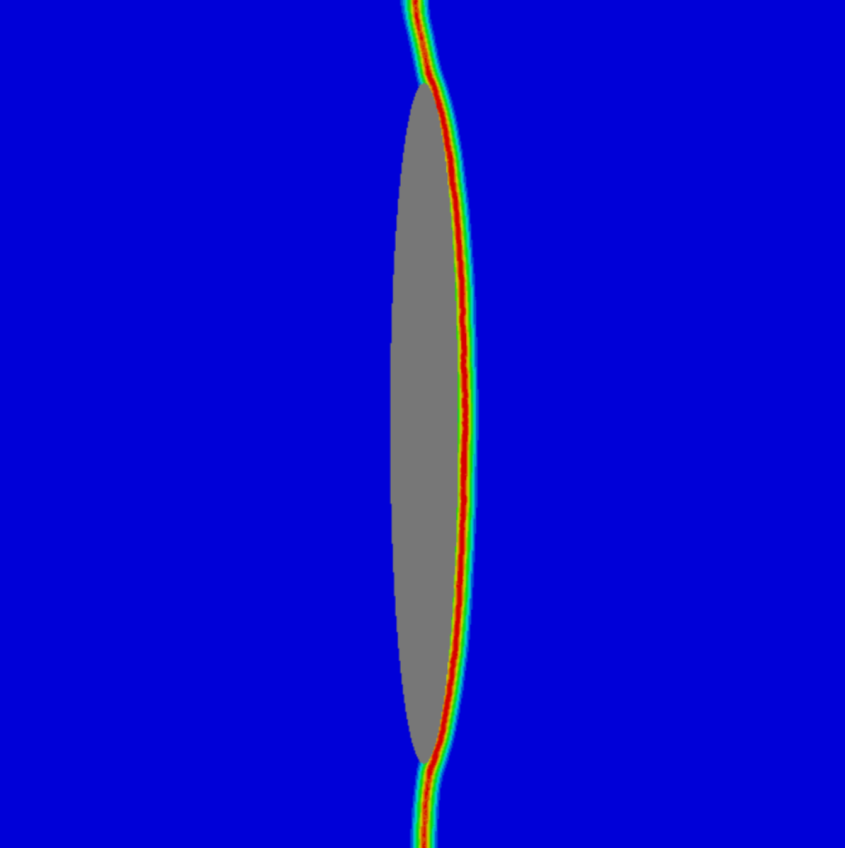
(a)

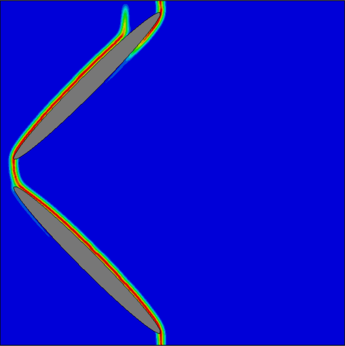
(b)

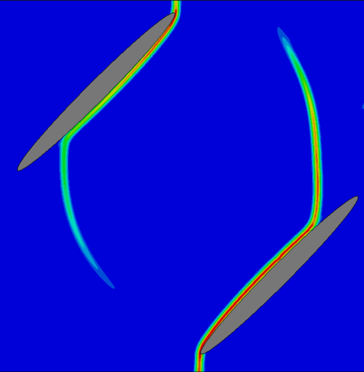
(c)

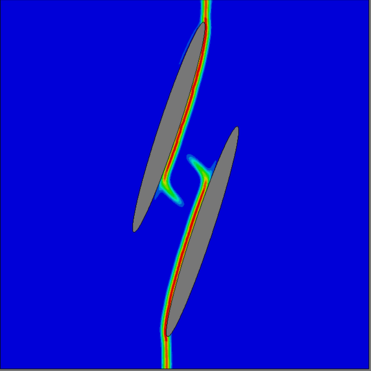
(d)

Figure 24: Effect of number of inclusions and their spatial distribution on simulated fracture paths. Two elliptical inclusion samples possess the identical volume fraction of inclusion and interface phase, mirroring the volume fractions in the single inclusion model.

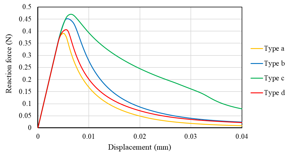
Figure 25: Calculated reaction force-displacement curve derived from the models illustrated in Figure 24

As can be seen in the second raw of Figure 24, the significant influence of the distribution of the aggregate and consequently the spatial distribution of the interface on the simulated fracture paths is evident. This influence is particularly evident in Figure 24(c), where the strategic placement of two aggregate particles resulted in the entire fracture of the sample occurring through two primary cracks. The formation and progression of these two primary cracks can significantly improve the fracture toughness of the material. As shown in Figure 25, the dissipated fracture energy ratio of the model shown in Figure 24(c) is approximately twice as high compared to the model with only one inclusion in Figure 24(a). This scenario demonstrates the potential to design composites with improved fracture characteristics by strategically positioning inclusions.

To gain a deeper insight into the mechanisms of crack initiation and propagation in multiphase materials, the reaction force-displacement curve of the model with two elliptical inclusions, as shown in Figure 24(b), is depicted in Figure 26. This curve is highlighted by four points, each representing specific regions of the reaction force-displacement curve. The stress and damage states corresponding to the individual points of the curve are shown in Figure 27. Looking at the second row of Figure 27, it is clear that the damage initially starts in the interface region. After propagating in this zone, it expands into the matrix as the specimen is further loaded. In addition, to explain the direction of crack propagation, the von Mises stress state is shown for each point. It can be seen that the crack propagates in areas where the stress is higher than in other areas of the specimen.

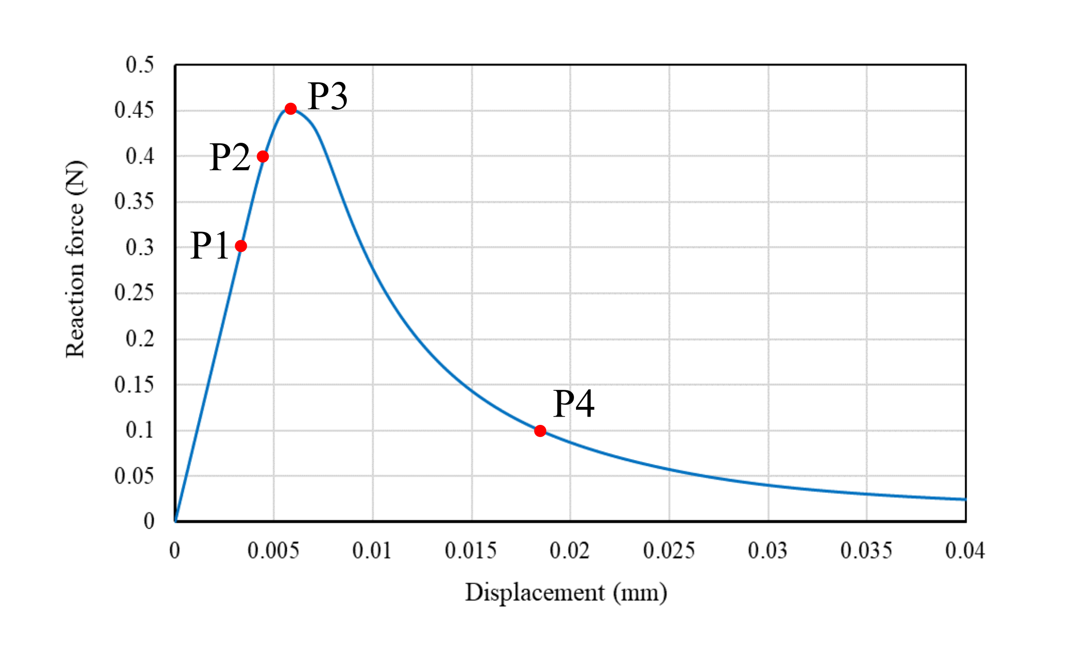
Figure 26: Calculated reaction force-displacement curve derived from the model with two elliptical inclusions. This model is shown in Figure 24(b). The force-displacement curve is provided with four different points, each representing a different phase of crack development, to analyze the stress and fracture conditions at each point.

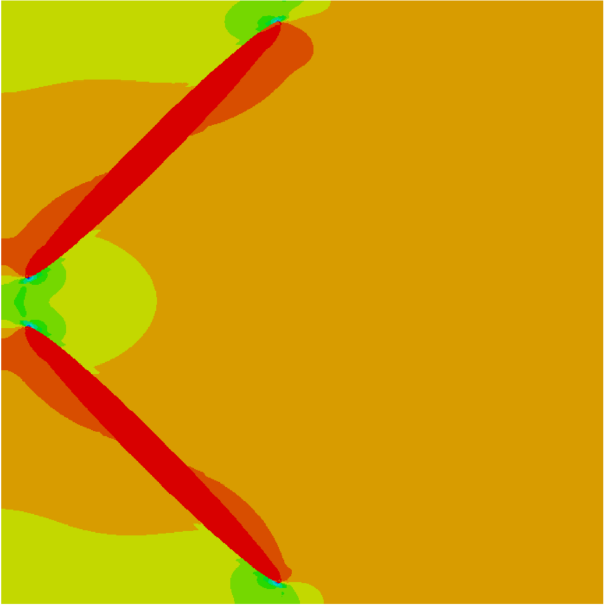
(a) Point P1

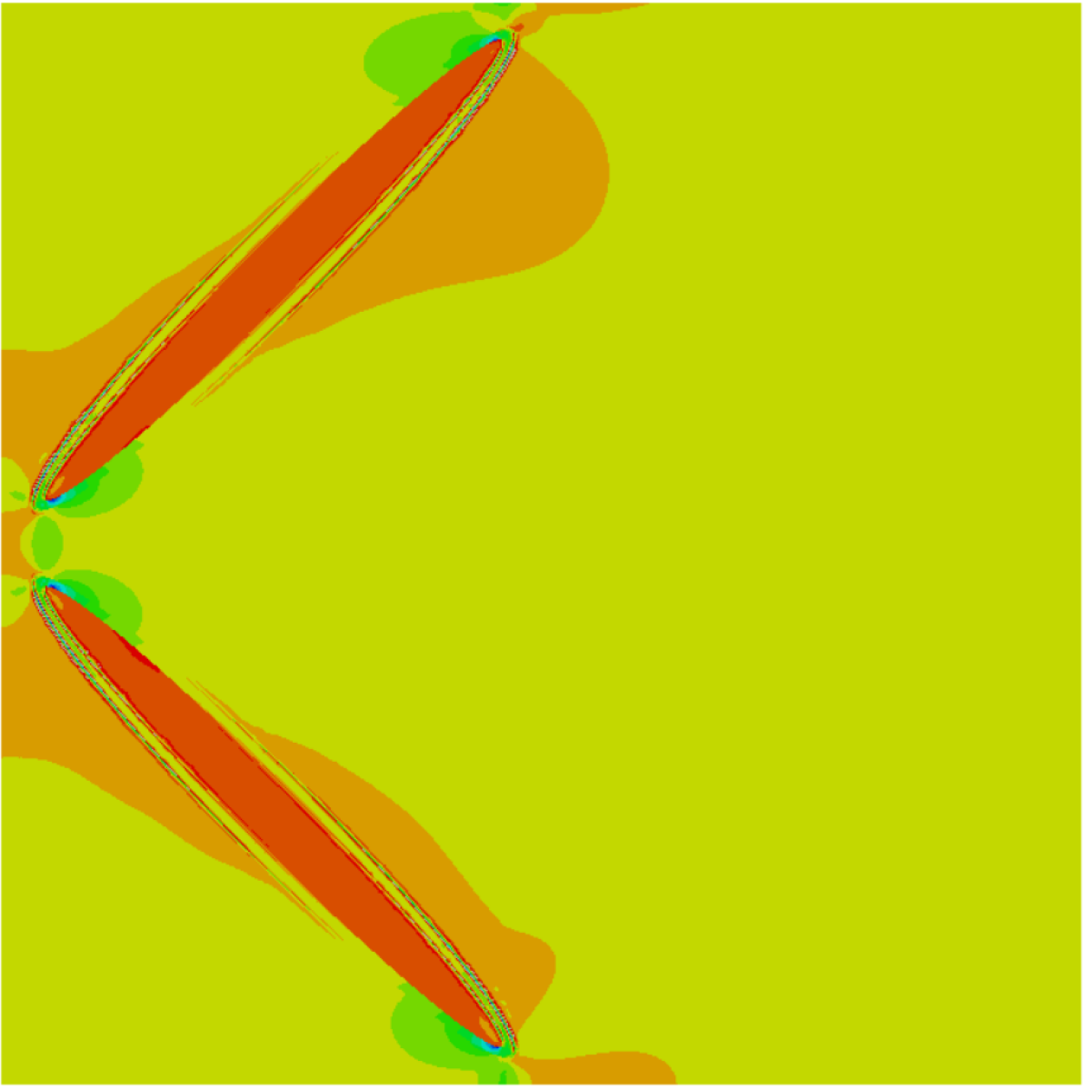
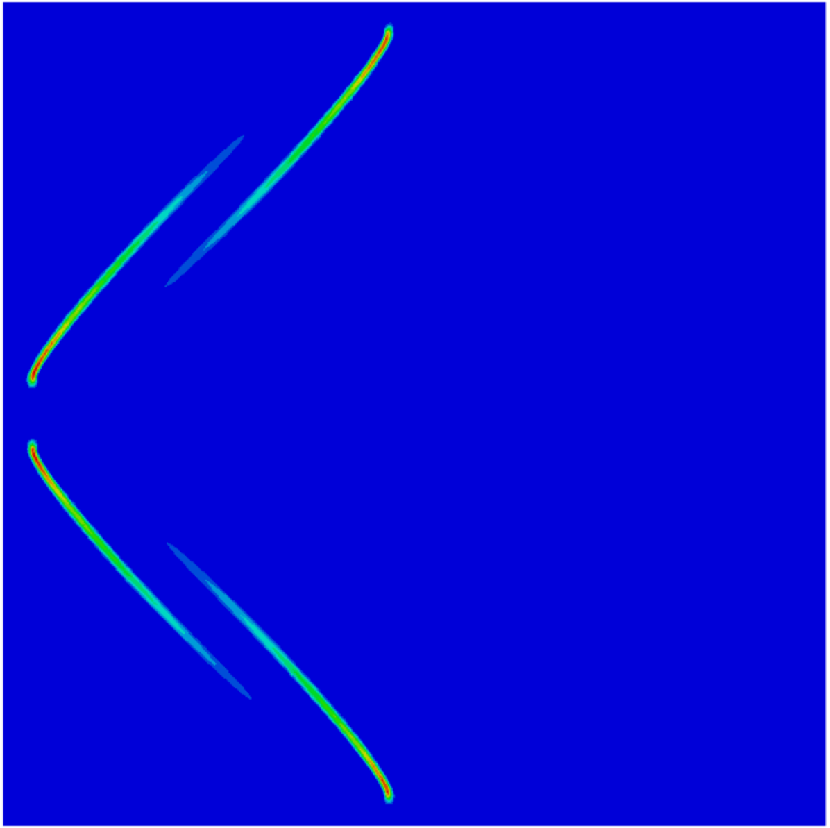
(b) Point P2

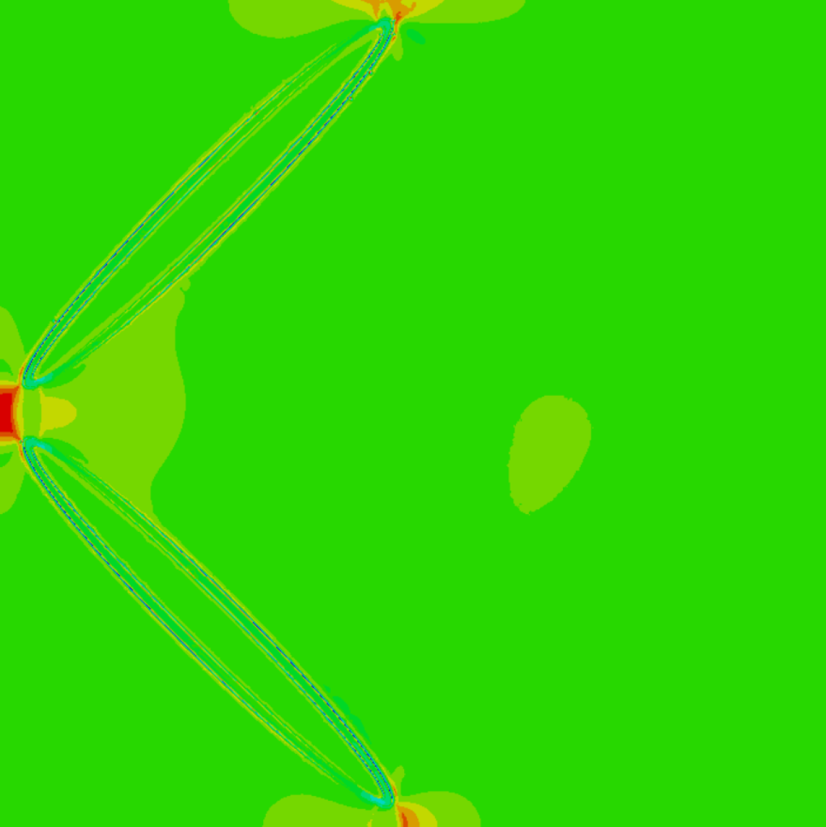
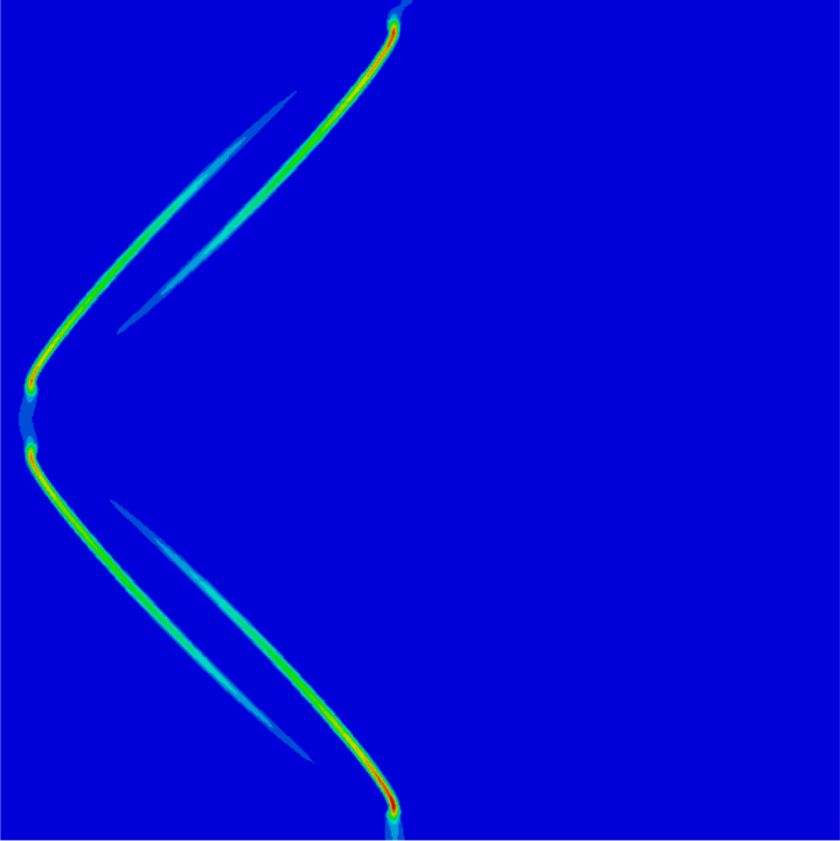
(c) Point P3

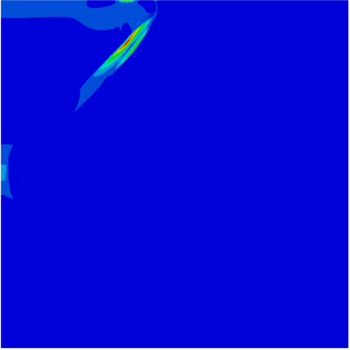
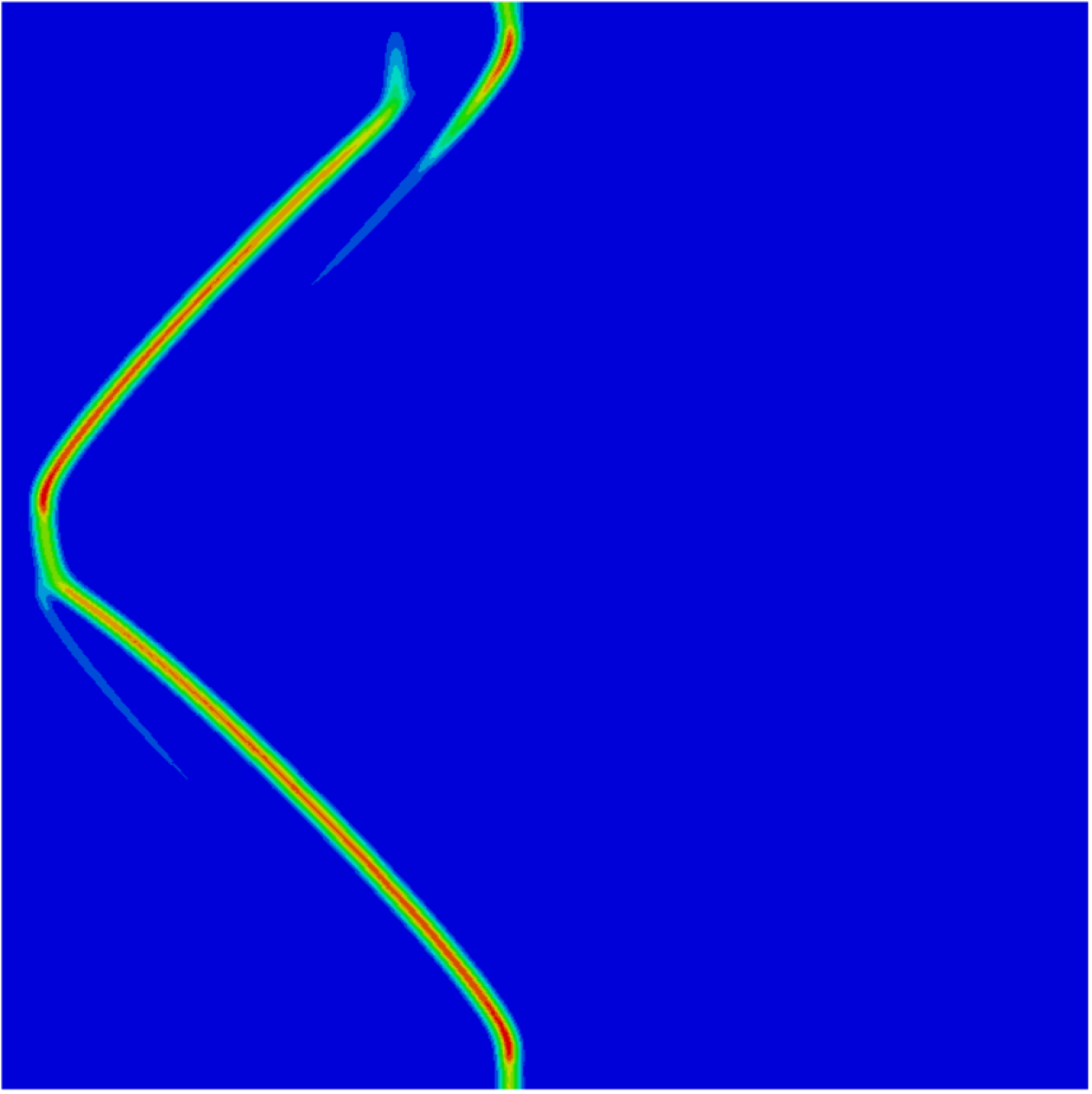
(d) Point P4

Figure 27: Stress state and fracture pathways corresponding to the points marked on the reaction force-displacement curve in Figure 26. The first row illustrates the von Mises stress, while the second row depicts the cohesive phase-field fracture variable. To better highlight stress concentrations in potential crack initiation zones, contour plots of local minimum and maximum von Mises stress values are presented. The specified local minimum and maximum von Mises stress for each frame are: (a) [0.62, 2.191] MPa, (b) [0.89, 3.02] MPa, (c) [0, 4.85] MPa, and (d) [0, 21] MPa.

4.5 Impact of Material Properties at Interface

To evaluate the influence of interface properties on the fracture behaviour of composite samples, three unique fracture properties for the interface zone have been identified and are detailed in Table 4. Interface 1 embodies significantly weakened fracture properties for the interface, whereas Interface 3 depicts a relatively strong Interface property. Interface 2 characterizes the fracture properties utilized in previous analysis

Table 4: Material properties of interface zone. Interface 1 signifies extremely weak interface attributes, Interface 2 corresponds to the properties used in earlier analyses in preceding sections, and Interface 3 denotes highly robust interface characteristics.

Phase	Fracture energy $G_{c}$ (N/mm)	Failure strength $\sigma_{u}$ (MPa)
Interface 1	0.008	1
Interface 2	0.02	2.4
Interface 3	0.4	6

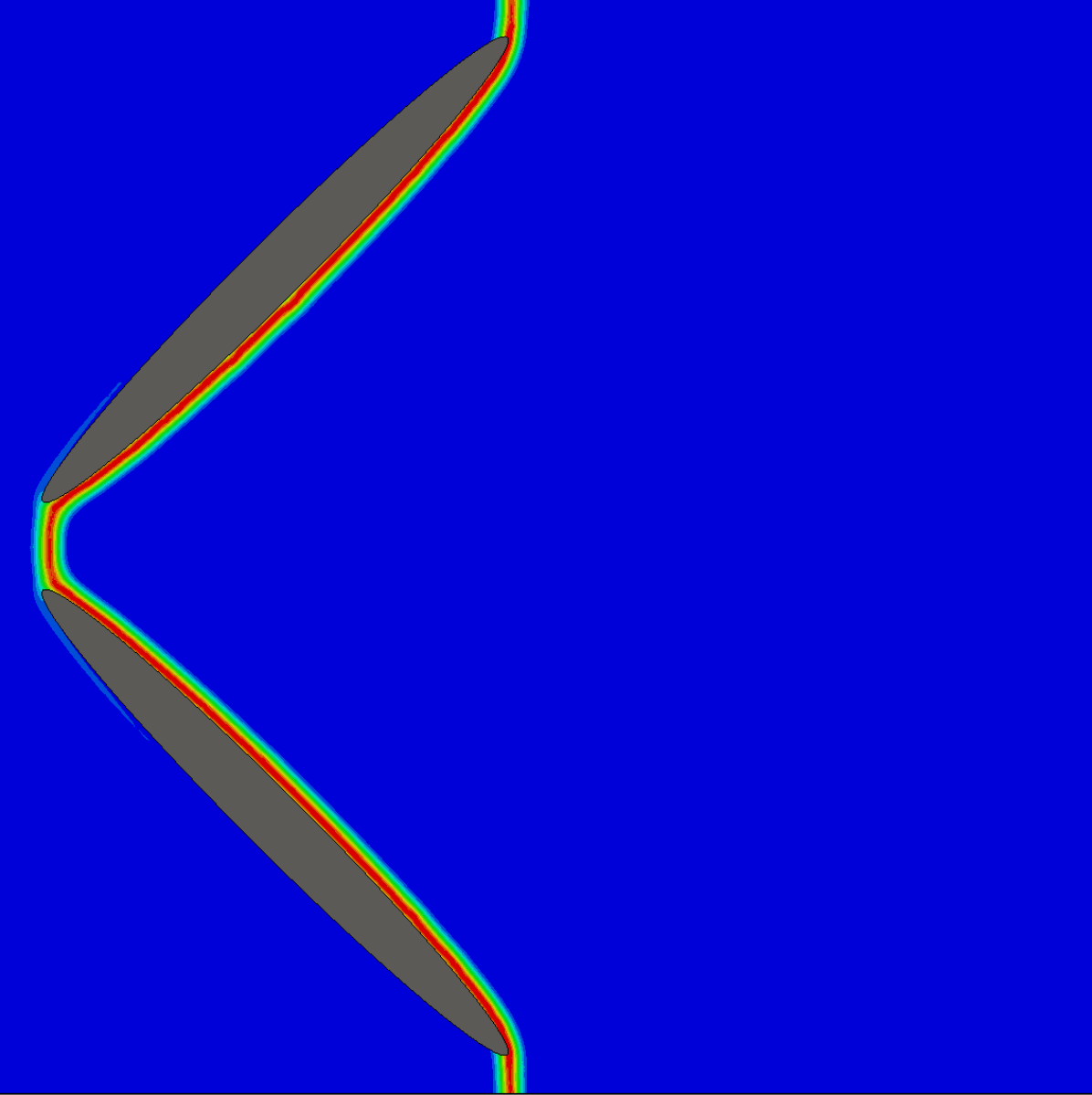
(a) Interface 1

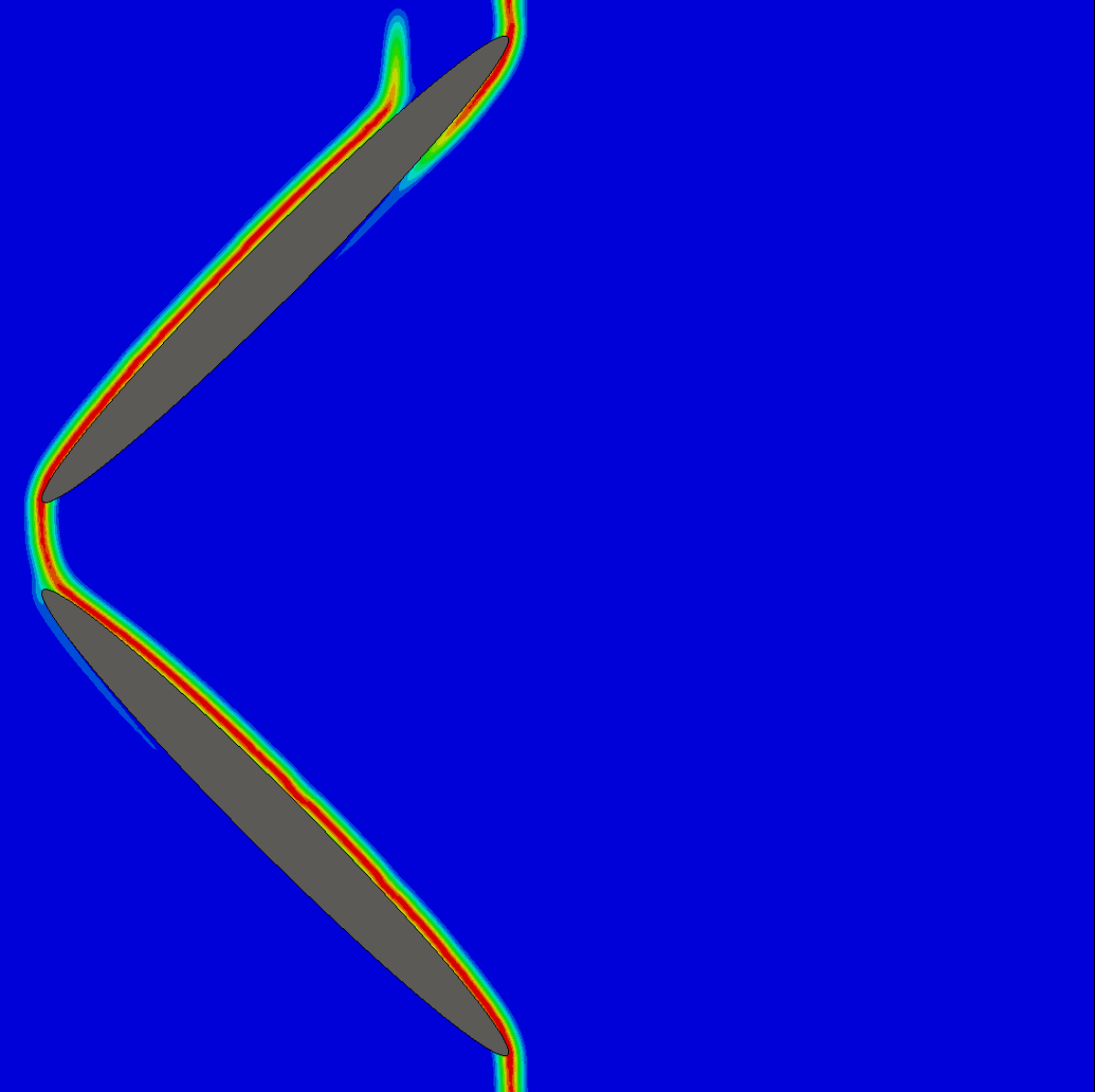
(b) Interface 2

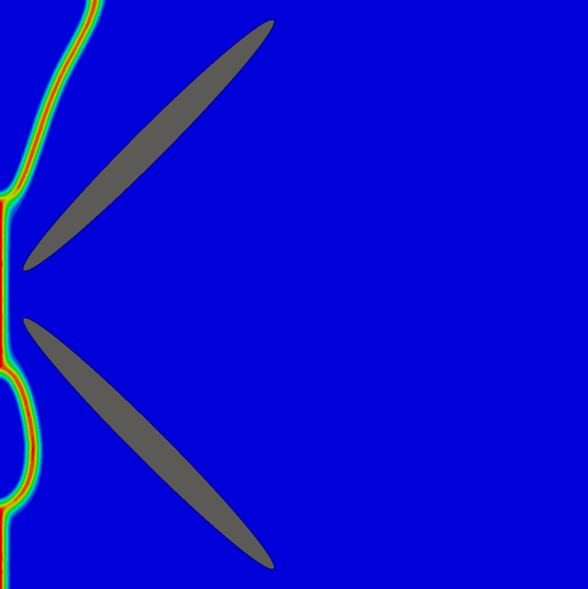
(c) Interface 3

Figure 28: Fracture paths in two unique microstructures that have an equivalent volume fraction of inclusion and interface phases. The material properties of the interface are provided in Table 4.

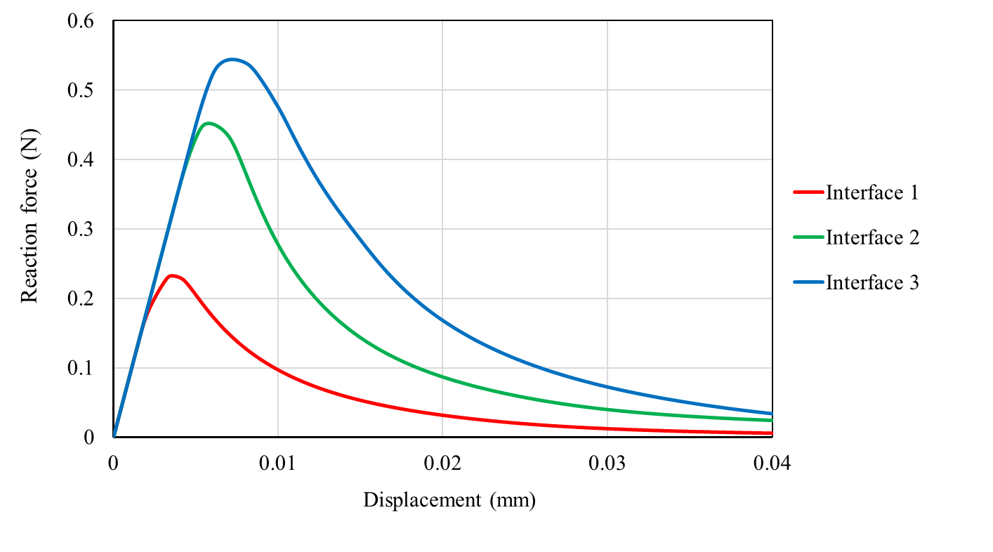
Figure 29: Force-displacement curves derived from FE simulations using distinct Interface properties as detailed in Table 4. While other material attributes are kept constant as specified in Table 3, only the properties of the interface are varied.

Figure 28 depicts the simulated fracture path for the two-inclusions scenario. As illustrated in Figure 28, by altering the interphase fracture properties, the crack path is deflected. Specifically, as depicted in Figure 28(b), altering the material properties of the interface zone results in subtle variations in the simulated fracture paths where two distinct crack paths can be observed, with one being notably shorter than the other. As depicted in Figure 29, the variations in fracture paths lead to a rise in the peak reaction force, subsequently causing greater energy dissipation upon full failure. The discrepancy in fracture paths is particularly evident in Figure 28(c), illustrating a marked change when employing very strong interface properties.

In the analysis performed in this section, two crucial insights are obtained: First, the role of morphological properties and their spatial distribution is central to the propagation of the fracture path. By influencing these factors, energy dissipation can be increased, which in turn improves the fracture properties of the material. Second, the importance of interface properties, which are often understudied in numerous studies, was highlighted. Altering these interface properties can influence the evolution of crack paths, potentially leading to increased peak reaction force.

5 Conclusion

In this study, four popular numerical models designed to simulate crack initiation and growth in heterogeneous solid materials with an interface phase have been analyzed in terms of their implementation complexities and computational costs. The four numerical methods examined are the standard phase-field fracture, cohesive phase-field fracture, cohesive zone model, and the hybrid model. In the hybrid model, the cohesive zone model is employed for interface debonding, while the cohesive phase-field fracture is utilized for matrix cracking. The findings were derived from a 2D single inclusion model, taking into account that the interface phase’s thickness is not significantly smaller than that of the other phases. The primary conclusions drawn from this research are:

• The SPFM approach doesn’t account for the cohesive behavior seen in semi-brittle materials within the softening zone. Also, the length scale parameter $l_{c}$ in the SPFM model is viewed as an intrinsic material property, which can be a drawback for small-scale simulations. Besides, the SPFM approach needs more computational resources, since a finer mesh is essential to capture the $l_{c}$ value accurately in the model compared to other methods examined in this work.

• The CPFM model is identified as a suitable numerical method for multiphase materials, especially when the interface thickness isn’t much smaller than the other phases. In the CPFM method, the length scale parameter acts as a numerical property, making it apt for small-scale simulations. Moreover, it’s observed that the CPFM model is computationally less demanding and is simpler to implement compared to hybrid fracture approach.

• The design of composites with targeted properties can be enabled by adjusting the arrangement of inclusions, modifying the interface property, or employing a combination of both. In this study, it is shown that a significant enhancement in the fracture toughness of the material can be achieved by strategically arranging inclusions or interface properties while keeping all other parameters constant.

It should be noted that in situations where the thickness of the interface is much smaller than that of the other phases, the hybrid model could be the most appropriate numerical method for fracture simulation in heterogeneous materials. This is mainly due to the fact that extremely thin interfaces require a very fine mesh size in FE simulations to accurately represent the interface for fracture models such as the cohesive phase-field fracture method. An alternative approach is to artificially increase the thickness of the interface by scaling its properties to enable the application of the CPFM model. This modification makes the CPFM model width insensitive, which could make it a unified fracture model for multiphase materials with isotropic phases. More information on this topic, including recent research, can be found in the paper by [61].

Table 5: Comparison of different fracture approaches for heterogeneous materials.

	Cohesive Zone Model	Standard Phase-field Fracture	Cohesive Phase-field Fracture	Hybrid Model
Stability	Low	High	Very high	High
Computational cost	Very High	High	Moderate	High
Implementation complexity	Very high	Low	Low	Very high
Main limitation	- Very high computational cost - High implementation complexity - Mesh-dependent crack path for bulk fracture	- High computational cost - Sensitivity to $l_{c}$ - Potentially not appropriate for very thin interface	- Potentially not appropriate for very thin interface	- High computational cost - High implementation complexity
Main advantage	- Simple formulation (esp. mode-dependency) - Suitable for interface fracture	-Arbitrary crack paths - Low implementation complexity	-Arbitrary crack paths - Moderate computational cost - Low implementation complexity	- Appropriate for very thin interface phase - Capturing mode-dependency at interface

5.1 Future development

Among the fracture models analyzed, the CPFM approach stands out as the preferred simulation method for heterogeneous multiphase solids where where the thickness of the interface is not significantly smaller than that of the other phases. This preference is due to its mesh insensitivity and more physically accurate nature, along with simpler implementation and lower computational costs. A future development could therefore be microstructural optimization with particular emphasis on advanced fracture properties, as well as the application of data-driven surrogate modeling techniques to predict mechanical properties and fracture paths by implementing CPFM approach. It is important to recognize that there are numerous other methods for simulating fractures in heterogeneous materials that are not compared in this work. Among the various methods, two important methods are finite cohesive zone modeling techniques and some special PFM methods in which interface debonding is model by using PFM approaches. Another direction for future research could therefore be a more comprehensive comparison of different and more sophisticated models. This would address some of the limitations of the classical CZM and standard phase-field fracture models implemented in the current work and potentially lead to more effective and accurate simulations. Table 5 provides a concise comparison of the various approaches, highlighting their advantages and limitations.

Declarations

The authors declare no conflict of interest

Appendix A Finite element implementation

The incorporation of the phase-field problem into the framework of the finite element method is achieved by employing the weak forms of Equation 16 and Equation 18 as

$$\begin{cases}\displaystyle\delta_{\mathrm{u}}P_{\mathrm{total}}=\int_{\Omega}\mathbb{\sigma}:\delta\mathbb{\varepsilon}\,\mathrm{dV}-\int_{\Omega}\mathbb{b^{*}}\cdot\delta\mathbb{u}\,\mathrm{d\Omega}-\int_{\Omega}\mathbb{t^{*}}\cdot\delta\mathbb{u}\,\mathrm{d\Omega}=0,&\text{}\\[10.0pt] \displaystyle\delta_{\mathrm{\phi}}P_{\mathrm{total}}=\int_{\Omega}\left[\omega^{\prime}(\phi)\,H+G_{c}\,\delta\gamma(\phi,\nabla_{\!\underaccent{\tilde}{x}}\phi)\right]\,\mathrm{dV}=0.&\text{}\\ \end{cases}$$ (37)

The field variables, namely $\bm{u}$ representing the displacement field and $\phi$ representing the phase-field parameter, can be discretized

$$u=\sum_{i=1}^{n}\mathbb{N_{i}}^{u}\mathbb{u_{i}},\qquad\phi=\sum_{i=1}^{n}\mathbb{N_{i}}^{\phi}\mathbb{\phi_{i}},$$ (38)

here, $\mathbb{N^{u}}$ and $\mathbb{N^{\phi}}$ denote the shape function matrices associated with the displacement and phase-field variables, respectively, and can be expressed as

$$\mathbb{N}^{u} =\begin{bmatrix}N_{1}&0&\ldots&N_{n}&0\\ 0&N_{1}&\ldots&0&N_{n}\end{bmatrix},$$ (39)

$$\mathbb{N}^{\phi} =\begin{bmatrix}N_{1}&N_{2}&\ldots&N_{n}\end{bmatrix},$$

where $n$ represents the total number of nodes within the FE model.

The gradients of field variables can be computed according to

$$\bm{\varepsilon}=\left[\nabla_{\!\underaccent{\tilde}{x}}\underaccent{\tilde}{\bm{u}}\right]^{\text{sym}}=\sum_{i=1}^{n}\mathbb{B_{i}}^{u}\mathbb{u_{i}},\qquad\nabla_{\!\underaccent{\tilde}{x}}\phi=\sum_{i=1}^{n}\mathbb{B_{i}}^{\phi}\mathbb{\phi_{i}},$$ (40)

where $\mathbb{B}^{u}$ and $\mathbb{\nabla}_{\!\underaccent{\tilde}{x}}{B}^{\phi}$ are the derivatives of the shape functions. In the 2D state, they are represented as

$$\mathbb{B}^{u}=\begin{bmatrix}\frac{\partial N_{1}}{\partial x}&0&\cdots&\frac{\partial N_{n}}{\partial x}&0\\[5.0pt] 0&\frac{\partial N_{1}}{\partial y}&\cdots&0&\frac{\partial N_{n}}{\partial y}\\[5.0pt] \frac{\partial N_{1}}{\partial y}&\frac{\partial N_{1}}{\partial x}&\cdots&\frac{\partial N_{n}}{\partial y}&\frac{\partial N_{n}}{\partial x}\end{bmatrix},$$ (41)

$$\mathbb{B}^{\phi}=\begin{bmatrix}\frac{\partial N_{1}}{\partial x}&\frac{\partial N_{2}}{\partial x}&\cdots&\frac{\partial N_{n}}{\partial x}\\[5.0pt] \frac{\partial N_{1}}{\partial y}&\frac{\partial N_{2}}{\partial y}&\cdots&\frac{\partial N_{n}}{\partial y}\end{bmatrix}.$$

As a result, the discretized weak form of the phase-field fracture problem takes the form

$$\begin{cases}\displaystyle\bm{R}^{u}=\int_{\Omega}\left(\bm{B}^{u}\right)^{T}\bm{\sigma}\,\mathrm{dV}-\int_{\Omega}\left(\bm{N}^{u}\right)^{T}\bm{b^{*}}\,\mathrm{d\Omega}-\int_{\Omega}\left(\bm{N}^{u}\right)^{T}\bm{t^{*}}\,\mathrm{dS}=0,&\text{}\\[10.0pt] \displaystyle\bm{R}^{\phi}=\int_{\Omega}\left\{\left(\bm{N}^{\phi}\right)^{T}\left[\omega^{\prime}(\phi)H+\frac{G_{c}}{c_{0}l_{c}}\alpha^{\prime}(\phi)\right]+\frac{2l_{c}G_{c}}{c_{0}}\left(\bm{B}^{\phi}\right)^{T}\bm{B}^{\phi}\bm{\phi}\right\}\,\mathrm{dV}=0,&\text{}\\ \end{cases}$$ (42)

where $\mathbb{R}^{u}$ and $\mathbb{R}^{\phi}$ represent the residual vectors associated with the displacement and phase-field variables, respectively. In this research, we employ the staggered scheme proposed by Gergely et al. [90] to solve the system of equations. The following residual vectors are resolved by staggered manner

$$\begin{bmatrix}\displaystyle\mathbb{K_{uu}}&\displaystyle\mathbb{0}\\ \displaystyle\mathbb{0}&\displaystyle\mathbb{K_{\phi\phi}}\end{bmatrix}\begin{Bmatrix}\displaystyle\mathbb{u}\\ \displaystyle\bm{\phi}\end{Bmatrix}=\begin{Bmatrix}\displaystyle\mathbb{R_{u}}\\ \displaystyle\mathbb{R_{\phi}}\end{Bmatrix},$$ (43)

where the stiffness matrix is computed as

$$\begin{cases}\displaystyle\bm{K}_{\mathrm{uu}}=\frac{\partial\bm{R}_{u}}{\partial\bm{u}}=\int_{\Omega}\left(\bm{B}^{u}\right)^{T}\left(\frac{\partial\bm{\sigma}}{\partial\bm{\varepsilon}}\right)\bm{B}^{u}\,\mathrm{dV},&\text{}\\[10.0pt] \displaystyle\bm{K}_{\mathrm{\phi\phi}}=\frac{\partial\bm{R}_{\phi}}{\partial\bm{\phi}}=\int_{\Omega}\left[\left(\bm{N}^{\phi}\right)^{T}\left[\omega^{\prime\prime}(\phi)\,H+\frac{G_{c}}{c_{0}\,l_{c}}\,\alpha^{\prime\prime}(\phi)\right]\bm{N}^{\phi}+\frac{2\,l_{c}\,G_{c}}{c_{0}}\left(\bm{B}^{\phi}\right)^{T}\bm{B}^{\phi}\right]\,\mathrm{dV},&\text{}\\ \end{cases}$$ (44)

where, $\mathbb{K}_{\mathrm{uu}}$ represents the stiffness matrix for the displacement field variable, while $\mathbb{K}_{\mathrm{\phi\phi}}$ corresponds to the stiffness matrix for the phase-field variable.

Appendix B Effect of coarse mesh in SPFM

The subsequent figure illustrates the consequences of selecting an unsuitable mesh size on the results derived from the benchmark model by implementing standard phase-field fracture approach. This result is achieved by employing the distinct material properties and boundary conditions specified in this study.

Appendix C Mesh convergence study

The mesh convergence analysis was conducted using the dual-inclusion model (refer to Figure 24(b)), maintaining a constant $l_{c}=0.3$ mm for all simulations across various mesh sizes. As observed in Figure 31, the fracture paths produced in all simulations exhibit consistent results, demonstrating a unique outcome for each mesh size.

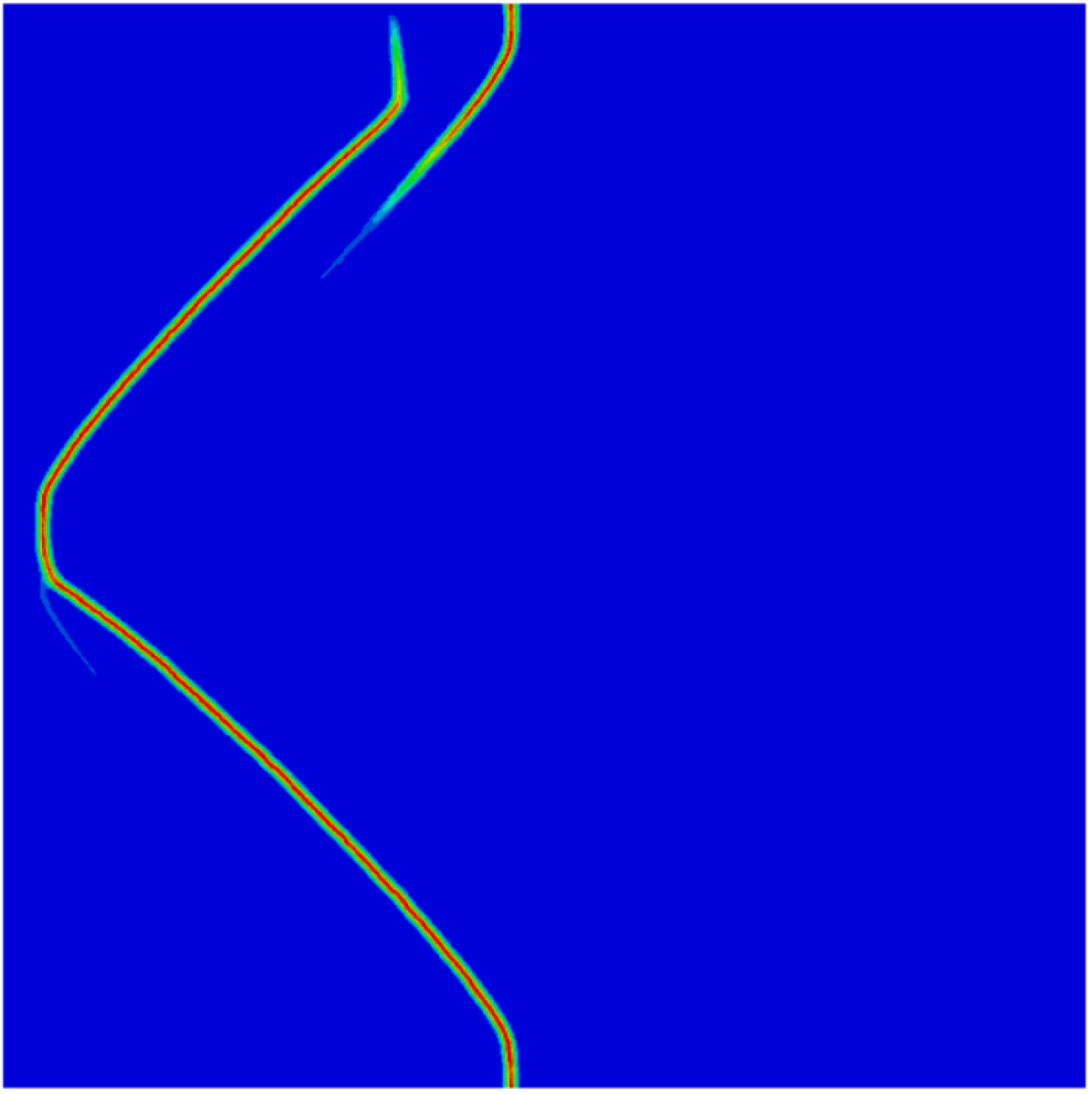
(a) Mesh 0.1 mm

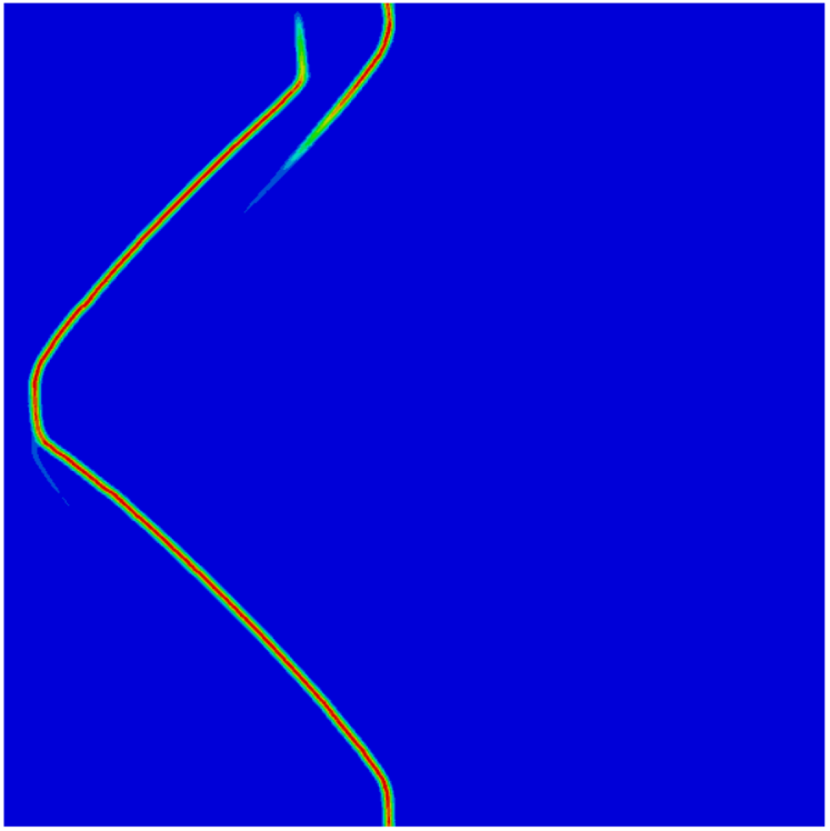
(b) Mesh 0.125 mm

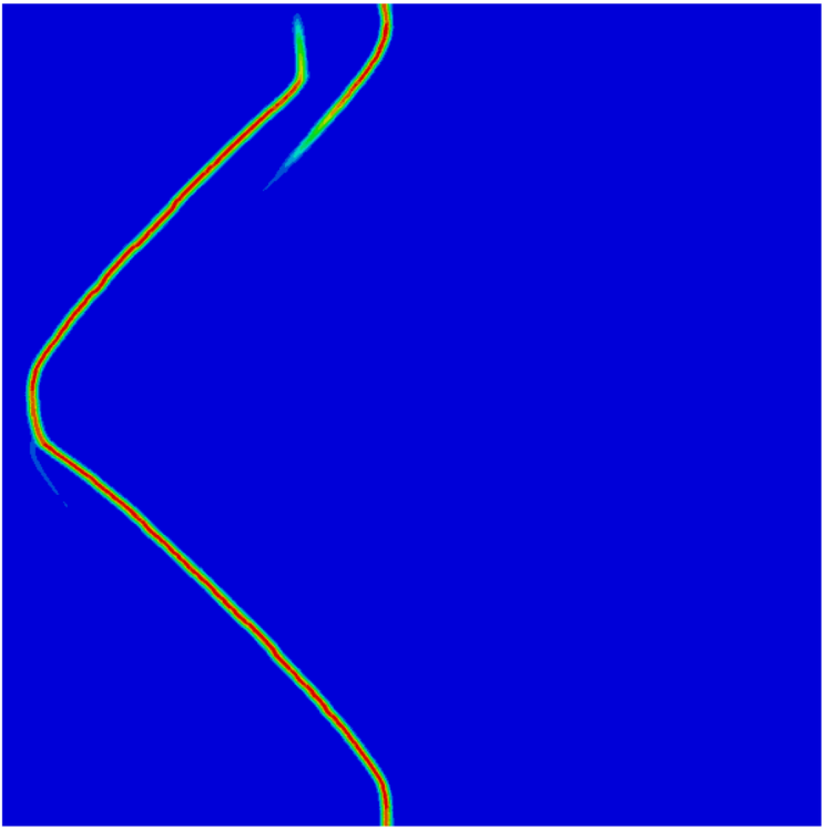
(c) Mesh 0.15 mm

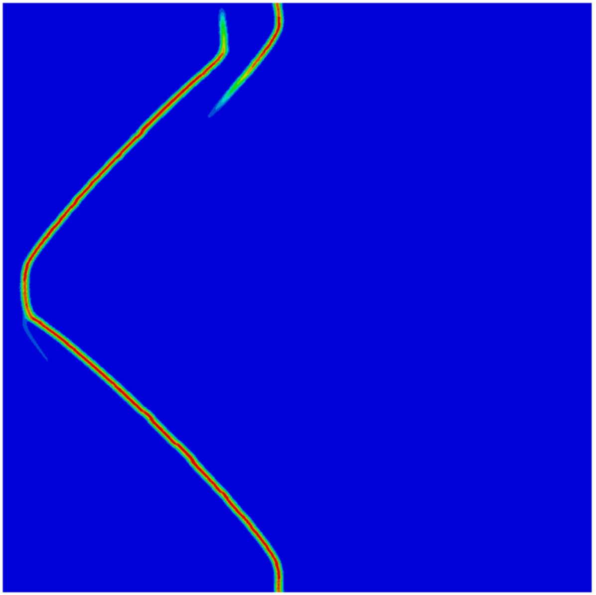
(d) Mesh 0.2 mm

Figure 31: Simulated fracture paths in a dual-inclusion elliptical model: This visualization showcases the fracture paths generated by the model, which is discretized using four distinct mesh sizes.

Figure 32 displays the reaction force-displacement results obtained from four different mesh sizes. The reaction force is calculated by summing the reaction forces at each node located on the left-hand side vertical edge. As evident from Figure 32, there is a high degree of correlation between the curves derived from the various mesh sizes, indicating a strong match in the outcomes.

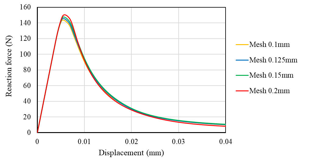
Figure 32: Reaction force-displacement from dual-inclusion elliptical model with four mesh sizes: This graph illustrates the reaction force, calculated by summing the forces at all nodes on the model’s vertical left edge, across varying mesh sizes.

Table 6 presents the total number of elements corresponding to different mesh sizes.

Table 6: Total number of elements in the dual-inclusion elliptical model, discretized at four distinct mesh sizes.

Mesh size (mm)	Total number of elements
0.1	278,407
0.125	178,795
0.15	124,181
0.2	77,158

References

- \bibcommenthead
- Unger and Eckardt [2011] Unger, J.F., Eckardt, S.: Multiscale modeling of concrete: from mesoscale to macroscale. Archives of computational Methods in Engineering 18, 341–393 (2011)
- Francfort and Marigo [1998] Francfort, G.A., Marigo, J.-J.: Revisiting brittle fracture as an energy minimization problem. Journal of the Mechanics and Physics of Solids 46(8), 1319–1342 (1998)
- Bourdin et al. [2000] Bourdin, B., Francfort, G.A., Marigo, J.-J.: Numerical experiments in revisited brittle fracture. Journal of the Mechanics and Physics of Solids 48(4), 797–826 (2000)
- Dugdale [1960] Dugdale, D.S.: Yielding of steel sheets containing slits. Journal of the Mechanics and Physics of Solids 8(2), 100–104 (1960)
- Barenblatt [1962] Barenblatt, G.I.: The mathematical theory of equilibrium cracks in brittle fracture. Advances in applied mechanics 7, 55–129 (1962)
- Park and Paulino [2011] Park, K., Paulino, G.H.: Cohesive zone models: a critical review of traction-separation relationships across fracture surfaces. Applied Mechanics Reviews 64(6), 060802 (2011)
- Borden et al. [2012] Borden, M.J., Verhoosel, C.V., Scott, M.A., Hughes, T.J., Landis, C.M.: A phase-field description of dynamic brittle fracture. Computer Methods in Applied Mechanics and Engineering 217, 77–95 (2012)
- Shen et al. [2018] Shen, Y., Mollaali, M., Li, Y., Ma, W., Jiang, J.: Implementation details for the phase field approaches to fracture. Journal of Shanghai Jiaotong University (Science) 23, 166–174 (2018)
- Bui and Hu [2021] Bui, T.Q., Hu, X.: A review of phase-field models, fundamentals and their applications to composite laminates. Engineering Fracture Mechanics 248, 107705 (2021)
- Wu et al. [2020] Wu, J.-Y., Nguyen, V.P., Nguyen, C.T., Sutula, D., Sinaie, S., Bordas, S.P.: Phase-field modeling of fracture. Advances in applied mechanics 53, 1–183 (2020)
- Wu et al. [2023] Wu, Z., Guo, L., Hong, J.: Improved staggered algorithm for phase-field brittle fracture with the local arc-lengthmethod. CMES-Computer Modeling in Engineering & Sciences 134(1) (2023)
- De Borst [2022] De Borst, R.: Fracture and damage in quasi-brittle materials: A comparison of approaches. Theoretical and Applied Fracture Mechanics 122, 103652 (2022)
- Yu et al. [2023] Yu, Y., Hou, C., Zheng, X., Rabczuk, T., Zhao, M.: A generally variational phase field model of fracture. Theoretical and Applied Fracture Mechanics 128, 104111 (2023)
- Liu et al. [2023] Liu, Y., Zhou, R., Lu, Z., Cheng, C., Wang, W.: Mesoscale modelling on the evolution of the fracture process zone in concrete using a unified phase-field approach: Size effect study. Theoretical and Applied Fracture Mechanics 128, 104110 (2023)
- Cavuoto et al. [2022] Cavuoto, R., Lenarda, P., Misseroni, D., Paggi, M., Bigoni, D.: Failure through crack propagation in components with holes and notches: An experimental assessment of the phase field model. International Journal of Solids and Structures 257, 111798 (2022)
- Miehe et al. [2010] Miehe, C., Welschinger, F., Hofacker, M.: Thermodynamically consistent phase-field models of fracture: Variational principles and multi-field fe implementations. International journal for numerical methods in engineering 83(10), 1273–1311 (2010)
- Harandi et al. [2023] Harandi, A., Tabib, M., Alatassi, B., Brepols, T., Rezaei, S., Reese, S.: A comparative study between phase-field and micromorphic gradient-extended damage models for brittle fracture. PAMM 22(1), 202200192 (2023)
- Conti et al. [2016] Conti, S., Focardi, M., Iurlano, F.: Phase field approximation of cohesive fracture models. In: Annales de l’Institut Henri Poincaré C, Analyse Non Linéaire, vol. 33, pp. 1033–1067 (2016). Elsevier
- Wu [2017] Wu, J.-Y.: A unified phase-field theory for the mechanics of damage and quasi-brittle failure. Journal of the Mechanics and Physics of Solids 103, 72–99 (2017)
- Geelen et al. [2019] Geelen, R.J.M., Liu, Y., Hu, T., Tupek, M.R., Dolbow, J.E.: A phase-field formulation for dynamic cohesive fracture. Computer Methods in Applied Mechanics and Engineering 348, 680–711 (2019)
- Quintanas-Corominas et al. [2019] Quintanas-Corominas, A., Reinoso, J., Casoni, E., Turon, A., Mayugo, J.: A phase field approach to simulate intralaminar and translaminar fracture in long fiber composite materials. Composite Structures 220, 899–911 (2019)
- Fei and Choo [2021] Fei, F., Choo, J.: Double-phase-field formulation for mixed-mode fracture in rocks. Computer Methods in Applied Mechanics and Engineering 376, 113655 (2021)
- Rezaei et al. [2022] Rezaei, S., Harandi, A., Brepols, T., Reese, S.: An anisotropic cohesive fracture model: Advantages and limitations of length-scale insensitive phase-field damage models. Engineering Fracture Mechanics 261, 108177 (2022)
- Zhang et al. [2023] Zhang, C., Zhou, S., Xu, Y., Liu, R.: Phase field method of multi-mode fracture propagation in transversely isotropic brittle rock. Theoretical and Applied Fracture Mechanics 128, 104134 (2023)
- Kumar et al. [2022] Kumar, P.K.A.V., Dean, A., Reinoso, J., Paggi, M.: Nonlinear thermo-elastic phase-field fracture of thin-walled structures relying on solid shell concepts. Computer Methods in Applied Mechanics and Engineering 396, 115096 (2022)
- Rezaei et al. [2023] Rezaei, S., Okoe-Amon, J.N., Varkey, C.A., Asheri, A., Ruan, H., Xu, B.-X.: A cohesive phase-field fracture model for chemo-mechanical environments: Studies on degradation in battery materials. Theoretical and Applied Fracture Mechanics 124, 103758 (2023)
- Zhang et al. [2023] Zhang, B., Luo, J., Fang, Z., Huang, H.: Phase field study of the thermo-electro-mechanical fracture behavior of flexoelectric solids. Theoretical and Applied Fracture Mechanics 125, 103833 (2023)
- Valverde-González et al. [2022] Valverde-González, A., Martínez-Pañeda, E., Quintanas-Corominas, A., Reinoso, J., Paggi, M.: Computational modelling of hydrogen assisted fracture in polycrystalline materials. international journal of hydrogen energy 47(75), 32235–32251 (2022)
- Mandal et al. [2021a] Mandal, T.K., Nguyen, V.P., Wu, J.-Y.: Comparative study of phase-field damage models for hydrogen assisted cracking. Theoretical and Applied Fracture Mechanics 111, 102840 (2021)
- Mandal et al. [2021b] Mandal, T.K., Nguyen, V.P., Wu, J.-Y., Nguyen-Thanh, C., de Vaucorbeil, A.: Fracture of thermo-elastic solids: Phase-field modeling and new results with an efficient monolithic solver. Computer Methods in Applied Mechanics and Engineering 376, 113648 (2021)
- Miehe et al. [2015] Miehe, C., Hofacker, M., Schänzel, L.-M., Aldakheel, F.: Phase field modeling of fracture in multi-physics problems. part ii. coupled brittle-to-ductile failure criteria and crack propagation in thermo-elastic–plastic solids. Computer Methods in Applied Mechanics and Engineering 294, 486–522 (2015)
- Dittmann et al. [2020] Dittmann, M., Aldakheel, F., Schulte, J., Schmidt, F., Krüger, M., Wriggers, P., Hesch, C.: Phase-field modeling of porous-ductile fracture in non-linear thermo-elasto-plastic solids. Computer Methods in Applied Mechanics and Engineering 361, 112730 (2020)
- Ortiz and Pandolfi [1999] Ortiz, M., Pandolfi, A.: Finite-deformation irreversible cohesive elements for three-dimensional crack-propagation analysis. International Journal for Numerical Methods in Engineering 44(9), 1267–1282 (1999)
- Nguyen [2014] Nguyen, V.P.: Discontinuous galerkin/extrinsic cohesive zone modeling: Implementation caveats and applications in computational fracture mechanics. Engineering fracture mechanics 128, 37–68 (2014)
- Xu and Needleman [1994] Xu, X.-P., Needleman, A.: Numerical simulations of fast crack growth in brittle solids. Journal of the Mechanics and Physics of Solids 42(9), 1397–1434 (1994)
- Paggi and Wriggers [2011a] Paggi, M., Wriggers, P.: A nonlocal cohesive zone model for finite thickness interfaces–part i: mathematical formulation and validation with molecular dynamics. Computational Materials Science 50(5), 1625–1633 (2011)
- Paggi and Wriggers [2011b] Paggi, M., Wriggers, P.: A nonlocal cohesive zone model for finite thickness interfaces–part ii: Fe implementation and application to polycrystalline materials. Computational Materials Science 50(5), 1634–1643 (2011)
- Sane et al. [2018] Sane, A., Padole, P., Uddanwadiker, R.: Progressive failure evaluation of composite skin-stiffener joints using node to surface interactions and czm. CMES-Computer Modeling in Engineering & Sciences 115(2) (2018)
- Naghdinasab et al. [2018] Naghdinasab, M., Farrokhabadi, A., Madadi, H.: A numerical method to evaluate the material properties degradation in composite rves due to fiber-matrix debonding and induced matrix cracking. Finite Elements in Analysis and Design 146, 84–95 (2018)
- Abbas et al. [2023] Abbas, M., Bary, B., Jason, L.: A 3d mesoscopic frictional cohesive zone model for the steel-concrete interface. International Journal of Mechanical Sciences 237, 107819 (2023)
- Wang et al. [2022] Wang, B., Zhu, E., Zhang, Z.: Microscale fracture damage analysis of lightweight aggregate concrete under tension and compression based on cohesive zone model. Journal of Engineering Mechanics 148(2), 04021153 (2022)
- Güzel et al. [2023] Güzel, D., Kaiser, T., Menzel, A.: A thermo-electro-mechanically coupled cohesive zone formulation for predicting interfacial damage. European Journal of Mechanics-A/Solids 99, 104935 (2023)
- Özdemir et al. [2010] Özdemir, I., Brekelmans, W., Geers, M.: A thermo-mechanical cohesive zone model. Computational Mechanics 46, 735–745 (2010)
- Dekker et al. [2021] Dekker, R., Meer, F.P., Maljaars, J., Sluys, L.J.: A cohesive xfem model for simulating fatigue crack growth under various load conditions. Engineering Fracture Mechanics 248, 107688 (2021)
- Rezaei et al. [2017] Rezaei, S., Wulfinghoff, S., Reese, S.: Prediction of fracture and damage in micro/nano coating systems using cohesive zone elements. International Journal of Solids and Structures 121, 62–74 (2017)
- Paggi and Wriggers [2016] Paggi, M., Wriggers, P.: Node-to-segment and node-to-surface interface finite elements for fracture mechanics. Computer Methods in Applied Mechanics and Engineering 300, 540–560 (2016)
- Javili et al. [2017] Javili, A., Steinmann, P., Mosler, J.: Micro-to-macro transition accounting for general imperfect interfaces. Computer Methods in Applied Mechanics and Engineering 317, 274–317 (2017)
- Rezaei et al. [2020] Rezaei, S., Rezaei Mianroodi, J., Khaledi, K., Reese, S.: A nonlocal method for modeling interfaces: Numerical simulation of decohesion and sliding at grain boundaries. Computer Methods in Applied Mechanics and Engineering 362, 112836 (2020)
- Verhoosel and de Borst [2013] Verhoosel, C.V., Borst, R.: A phase-field model for cohesive fracture. International Journal for numerical methods in Engineering 96(1), 43–62 (2013)
- Nguyen et al. [2016] Nguyen, T.T., Yvonnet, J., Zhu, Q.-Z., Bornert, M., Chateau, C.: A phase-field method for computational modeling of interfacial damage interacting with crack propagation in realistic microstructures obtained by microtomography. Computer Methods in Applied Mechanics and Engineering 312, 567–595 (2016). Phase Field Approaches to Fracture
- Pillai et al. [2023] Pillai, A.U., Behera, A.K., Rahaman, M.M.: Combined diffused material interface and hybrid phase-field model for brittle fracture in heterogeneous composites. Engineering Fracture Mechanics 277, 108957 (2023)
- Hansen-Dörr et al. [2019] Hansen-Dörr, A.C., Borst, R., Hennig, P., Kästner, M.: Phase-field modelling of interface failure in brittle materials. Computer Methods in Applied Mechanics and Engineering 346, 25–42 (2019)
- Nguyen et al. [2016] Nguyen, T.-T., Yvonnet, J., Zhu, Q.-Z., Bornert, M., Chateau, C.: A phase-field method for computational modeling of interfacial damage interacting with crack propagation in realistic microstructures obtained by microtomography. Computer Methods in Applied Mechanics and Engineering 312, 567–595 (2016)
- Zhang et al. [2019] Zhang, P., Hu, X., Yang, S., Yao, W.: Modelling progressive failure in multi-phase materials using a phase field method. Engineering Fracture Mechanics 209, 105–124 (2019)
- Li et al. [2020a] Li, P., Yvonnet, J., Combescure, C.: An extension of the phase field method to model interactions between interfacial damage and brittle fracture in elastoplastic composites. International Journal of Mechanical Sciences 179, 105633 (2020)
- Li et al. [2020b] Li, G., Yin, B., Zhang, L., Liew, K.: Modeling microfracture evolution in heterogeneous composites: A coupled cohesive phase-field model. Journal of the Mechanics and Physics of Solids 142, 103968 (2020)
- Li et al. [2022] Li, W., Nguyen-Thanh, N., Zhou, K.: Phase-field modeling of interfacial debonding in multi-phase materials via an adaptive isogeometric-meshfree approach. Engineering Fracture Mechanics 269, 108481 (2022)
- Tarafder et al. [2020] Tarafder, P., Dan, S., Ghosh, S.: Finite deformation cohesive zone phase field model for crack propagation in multi-phase microstructures. Computational Mechanics 66(3), 723–743 (2020)
- Dhaladhuli et al. [2022] Dhaladhuli, P., Amirtham, R., Reddy, J.N.: Interaction between interfacial damage and crack propagation in quasi-brittle materials. Mechanics of Advanced Materials and Structures 29(22), 3187–3208 (2022)
- Nguyen-Thanh et al. [2022] Nguyen-Thanh, N., Li, W., Huang, J., Zhou, K.: Multi phase-field modeling of anisotropic crack propagation in 3d fiber-reinforced composites based on an adaptive isogeometric meshfree collocation method. Computer Methods in Applied Mechanics and Engineering 393, 114794 (2022)
- Zhou et al. [2022] Zhou, Q., Wei, Y., Zhou, Y., Yang, L.: An interface-width-insensitive cohesive phase-field model for fracture evolution in heterogeneous materials. International Journal of Solids and Structures 256, 111980 (2022)
- Yin et al. [2023] Yin, B., Akbar, A., Zhang, Y., Liew, K.: Modeling progressive failure and crack evolution in a randomly distributed fiber system via a coupled phase-field cohesive model. Composite Structures 313, 116959 (2023)
- Bian et al. [2024] Bian, P.-L., Qing, H., Schmauder, S., Yu, T.: A unified phase-field method-based framework for modeling quasi-brittle fracture in composites with interfacial debonding. Composite Structures 327, 117647 (2024)
- Kumar and Sain [2024] Kumar, A., Sain, T.: Modeling the interaction between intra and interlaminar cracking in frp composites using phase-field regularized interface fracture. Theoretical and Applied Fracture Mechanics 129, 104177 (2024)
- Nguyen et al. [2019] Nguyen, T.-T., Yvonnet, J., Waldmann, D., He, Q.-C.: Phase field modeling of interfacial damage in heterogeneous media with stiff and soft interphases. Engineering Fracture Mechanics 218, 106574 (2019)
- Paggi and Reinoso [2017] Paggi, M., Reinoso, J.: Revisiting the problem of a crack impinging on an interface: a modeling framework for the interaction between the phase field approach for brittle fracture and the interface cohesive zone model. Computer Methods in Applied Mechanics and Engineering 321, 145–172 (2017)
- Zhang et al. [2020] Zhang, P., Feng, Y., Bui, T.Q., Hu, X., Yao, W.: Modelling distinct failure mechanisms in composite materials by a combined phase field method. Composite Structures 232, 111551 (2020)
- Tan and Martinez-Paneda [2021] Tan, W., Martinez-Paneda, E.: Phase field predictions of microscopic fracture and r-curve behaviour of fibre-reinforced composites. Composites Science and Technology 202, 108539 (2021)
- Hu et al. [2023] Hu, Z., Suo, X., Wang, M., Jiang, F., Huang, H., Shen, Y.: A phase-field-cohesive-zone framework to simulate multiple failure mechanisms of elastoplastic fiber-reinforced composites. International Journal of Fracture, 1–17 (2023)
- Guillén-Hernández et al. [2019] Guillén-Hernández, T., García, I., Reinoso, J., Paggi, M.: A micromechanical analysis of inter-fiber failure in long reinforced composites based on the phase field approach of fracture combined with the cohesive zone model. International Journal of Fracture 220, 181–203 (2019)
- Guillén-Hernández et al. [2020] Guillén-Hernández, T., Quintana-Corominas, A., García, I., Reinoso, J., Paggi, M., Turón, A.: In-situ strength effects in long fibre reinforced composites: A micro-mechanical analysis using the phase field approach of fracture. Theoretical and Applied Fracture Mechanics 108, 102621 (2020)
- Han et al. [2023] Han, D., Liu, G., Xi, Y., Xia, X., Zhao, Y.: Simulation of low-temperature brittle fracture of asphalt mixtures based on phase-field cohesive zone model. Theoretical and Applied Fracture Mechanics 125, 103878 (2023)
- Le et al. [2015] Le, B., Yvonnet, J., He, Q.-C.: Computational homogenization of nonlinear elastic materials using neural networks. International Journal for Numerical Methods in Engineering 104(12), 1061–1084 (2015)
- Braides [1998] Braides, A.: Approximation of Free-discontinuity Problems vol. 1694. Springer, ??? (1998)
- Bourdin et al. [2008] Bourdin, B., Francfort, G.A., Marigo, J.-J.: The variational approach to fracture. Journal of elasticity 91, 5–148 (2008)
- Xia et al. [2021] Xia, Y., Wu, W., Yang, Y., Fu, X.: Mesoscopic study of concrete with random aggregate model using phase field method. Construction and Building Materials 310, 125199 (2021)
- Lancioni and Royer-Carfagni [2009] Lancioni, G., Royer-Carfagni, G.: The variational approach to fracture mechanics. a practical application to the french panthéon in paris. Journal of elasticity 95, 1–30 (2009)
- Amor et al. [2009] Amor, H., Marigo, J.-J., Maurini, C.: Regularized formulation of the variational brittle fracture with unilateral contact: Numerical experiments. Journal of the Mechanics and Physics of Solids 57(8), 1209–1229 (2009)
- Wu et al. [2020] Wu, J.-Y., Huang, Y., Nguyen, V.P.: On the bfgs monolithic algorithm for the unified phase field damage theory. Computer Methods in Applied Mechanics and Engineering 360, 112704 (2020)
- Pham et al. [2011] Pham, K., Amor, H., Marigo, J.-J., Maurini, C.: Gradient damage models and their use to approximate brittle fracture. International Journal of Damage Mechanics 20(4), 618–652 (2011)
- Barenblatt [1959] Barenblatt, G.I.: The formation of equilibrium cracks during brittle fracture. general ideas and hypotheses. axially-symmetric cracks. Journal of applied mathematics and mechanics 23(3), 622–636 (1959)
- Najafi Koopas et al. [2023] Najafi Koopas, R., Rauter, N., Lammering, R.: Two-dimensional mesoscale finite element modeling of concrete damage and failure. Applied Sciences 13(15), 8971 (2023)
- Hillerborg et al. [1976] Hillerborg, A., Modéer, M., Petersson, P.-E.: Analysis of crack formation and crack growth in concrete by means of fracture mechanics and finite elements. Cement and concrete research 6(6), 773–781 (1976)
- Xi et al. [2018] Xi, X., Yang, S., Li, C.-Q., Cai, M., Hu, X., Shipton, Z.K.: Meso-scale mixed-mode fracture modelling of reinforced concrete structures subjected to non-uniform corrosion. Engineering Fracture Mechanics 199, 114–130 (2018)
- Camanho and Dávila [2002] Camanho, P.P., Dávila, C.G.: Mixed-mode decohesion finite elements for the simulation of delamination in composite materials. Technical report (2002)
- Benzeggagh and Kenane [1996] Benzeggagh, M.L., Kenane, M.: Measurement of mixed-mode delamination fracture toughness of unidirectional glass/epoxy composites with mixed-mode bending apparatus. Composites science and technology 56(4), 439–449 (1996)
- Nguyen [2014] Nguyen, V.P.: An open source program to generate zero-thickness cohesive interface elements. Advances in Engineering Software 74, 27–39 (2014)
- Xiong and Xiao [2019] Xiong, X., Xiao, Q.: Meso-scale simulation of concrete based on fracture and interaction behavior. Applied Sciences 9(15), 2986 (2019)
- Wang et al. [2016] Wang, X., Zhang, M., Jivkov, A.P.: Computational technology for analysis of 3d meso-structure effects on damage and failure of concrete. International Journal of Solids and Structures 80, 310–333 (2016)
- Molnár and Gravouil [2017] Molnár, G., Gravouil, A.: 2d and 3d abaqus implementation of a robust staggered phase-field solution for modeling brittle fracture. Finite Elements in Analysis and Design 130, 27–38 (2017)
- Cornelissen et al. [1986] Cornelissen, H., Hordijk, D., Reinhardt, H.: Experimental determination of crack softening characteristics of normalweight and lightweight. Heron 31(2), 45–46 (1986)
- Nguyen et al. [2016] Nguyen, T.T., Yvonnet, J., Bornert, M., Chateau, C., Sab, K., Romani, R., Le Roy, R.: On the choice of parameters in the phase field method for simulating crack initiation with experimental validation. International Journal of Fracture 197, 213–226 (2016)
- Kuhn and Müller [2014] Kuhn, C., Müller, R.: Simulation of size effects by a phase field model for fracture. Theoretical and Applied Mechanics Letters 4(5), 051008 (2014)
- Bonifazi et al. [2015] Bonifazi, G., Capobianco, G., Serranti, S., Eggimann, M., Wagner, E., Di Maio, F., Lotfi, S.: The itz in concrete with natural and recycled aggregates: Study of microstructures based on image and sem analysis. Proc. 15th Euroseminar Microsc. Appl. to Build. Mater, 299–308 (2015)
- Rezaei et al. [2021] Rezaei, S., Mianroodi, J.R., Brepols, T., Reese, S.: Direction-dependent fracture in solids: Atomistically calibrated phase-field and cohesive zone model. Journal of the Mechanics and Physics of Solids 147, 104253 (2021)
- Paggi et al. [2018] Paggi, M., Corrado, M., Reinoso, J.: Fracture of solar-grade anisotropic polycrystalline silicon: A combined phase field–cohesive zone model approach. Computer Methods in Applied Mechanics and Engineering 330, 123–148 (2018)
- Ren et al. [2015] Ren, W., Yang, Z., Sharma, R., Zhang, C., Withers, P.J.: Two-dimensional x-ray ct image based meso-scale fracture modelling of concrete. Engineering Fracture Mechanics 133, 24–39 (2015)
- Singh et al. [2023] Singh, S., Pflug, L., Mergheim, J., Stingl, M.: On optimization of heterogeneous materials for enhanced resistance to bulk fracture. Forces in Mechanics 12, 100200 (2023)