Quantum control of continuous systems via nonharmonic potential modulation
Abstract
We present a theoretical proposal for preparing and manipulating a state of a single continuous-variable degree of freedom confined to a nonharmonic potential. By utilizing optimally controlled modulation of the potential’s position and depth, we demonstrate the generation of non-Gaussian states, including Fock, Gottesman-Kitaev-Preskill, multi-legged-cat, and cubic-phase states, as well as the implementation of arbitrary unitaries within a selected two-level subspace. Additionally, we propose protocols for single-shot orthogonal state discrimination and algorithmic cooling and analyze the robustness of this control scheme against noise. Since all the presented protocols rely solely on the precise modulation of the effective nonharmonic potential landscape, they are relevant to several experiments with continuous-variable systems, including the motion of a single particle in an optical tweezer or lattice, or current in circuit quantum electrodynamics.
The preparation of a continuous-variable system in a non-Gaussian quantum state is of paramount importance in various aspects of quantum science. This ranges from fundamental tests of quantum mechanics [1, 2, 3, 4, 5], through the design of quantum sensors [6, 7, 8, 9], to quantum information processing [10, 11, 12, 13, 14, 15, 16, 17, 18]. The generation of non-Gaussian states requires a nonlinear resource, often introduced through coupling to an auxiliary degree of freedom, such as a two-level system [19, 20, 12, 21, 15, 22, 5]. On the other hand, some continuous-variable systems already possess intrinsic nonlinearity in the potential of a canonical variable. Notable examples include the motion of a particle in a trap of finite depth [23, 24] and the current in an electric circuit with a Josephson junction [25]. These nonharmonicites in the potential are typically used to define a qubit within continuous-variable systems [26, 27, 28, 29, 30]. In contrast, here we explore methods for utilizing this intrinsic nonlinearity to generate and control states beyond the two-dimensional subspace.
More specifically, we develop protocols to generate a plethora of states, including Fock, Gottesman-Kitaev-Preskill (GKP) [10], multi-legged-cat [1, 31], and cubic-phase [10, 32], using optimal control [33, 34, 35] of the position and depth of the potential. In addition, we employ this control mechanism to design protocols that implement arbitrary unitaries in selected subspaces, enable single-shot orthogonal state discrimination, and perform algorithmic cooling [36]. These protocols could be implemented with single atoms in optical tweezers [37, 38, 39, 40, 41] and lattices [23, 42] to extend the motional states available in quantum protocols with itinerant particles, e.g., fermionic quantum processors [18]; or with flux-tunable transmons [28, 43, 25] for minimally invasive state manipulation [see Fig 1(a)]. Indeed, previous works, including control of Bose-Einstein condensates [44, 45, 46, 47], fast atom transport [48, 49, 42], ion shuttling [50], and Kerr-cat state creation through two-photon driving [51], have demonstrated similar concepts.
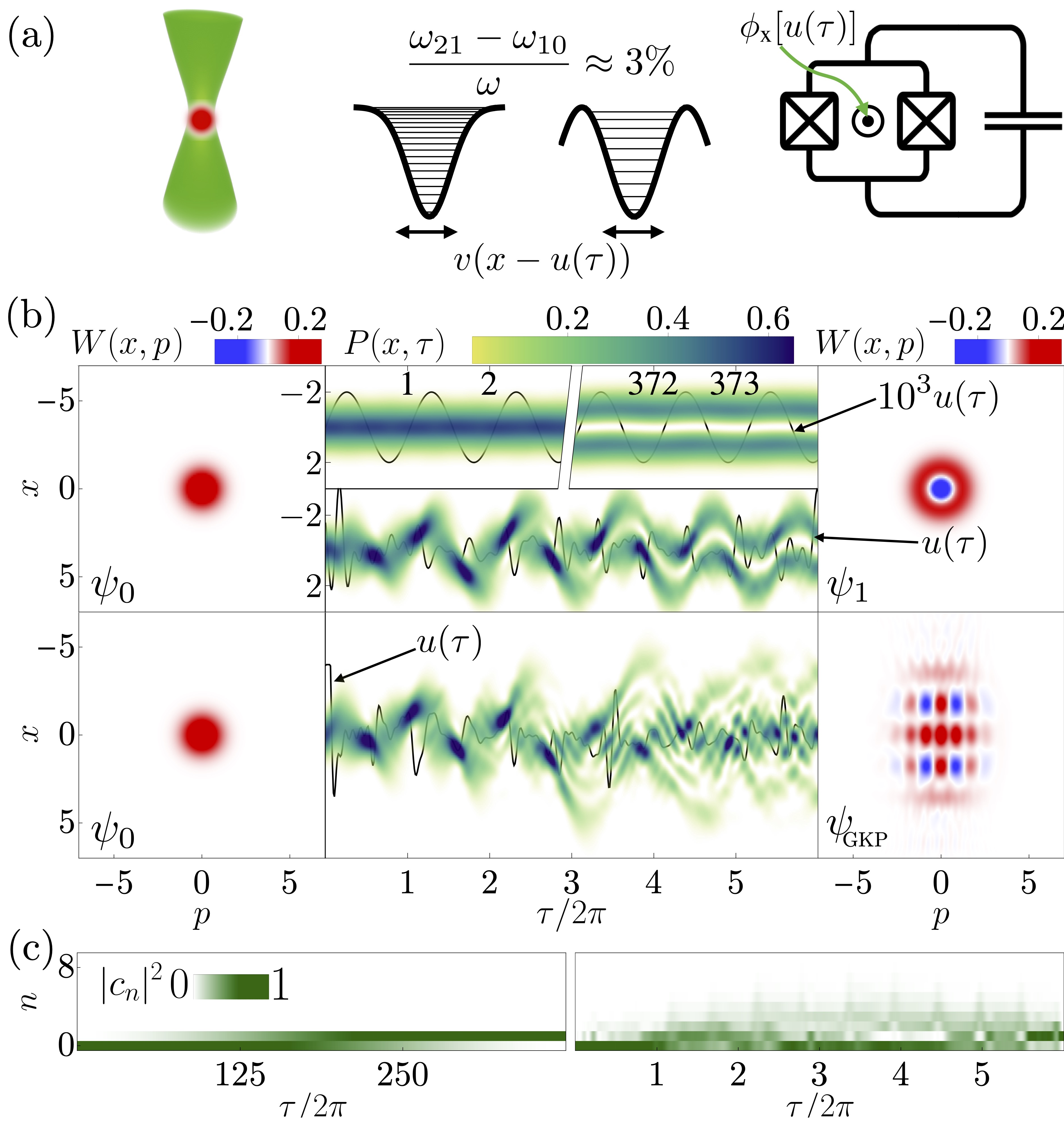
As a starting point, we focus on a one-dimensional continuous-variable system described by two conjugate quadrature operators, and , which may correspond to an arbitrary realization of a single mode, e.g., the motion of a single atom in an optical tweezer or a lattice, or phase and charge operators in a flux-tunable transmon (for particular mappings, cf. Supplemental Material (SM) [52]). In the leading order, each of these setups is harmonic with frequency , yielding natural time , canonical length , and momentum scales, where creates a single excitation. For an atom in a tweezer, we have , , and ; while for the flux-tunable transmon , , and . Here, is the mass of an atom, is the tweezer waist, is the tweezer depth, is the charge energy, and is the total Josephson energy. The system’s coherent dynamics is driven by a Hamiltonian,
| (1) |
where is the dimensionless potential. The shape of the potential is taken to be symmetric in , and we find it useful to express it as when expanded up to the second order in the small parameter . For the examples considered in this letter, the tweezer potential is Gaussian, , while for the flux-tunable transmon it is a cosine, and a squared sine for an optical lattice, . Note we have defined the units so that the functional forms of these potentials match up to the second leading order, allowing for a unified discussion of nonharmonicity. Here, is the measure of the nonharmonicity of the potential, comparing to the characteristic length scale of the potential, and translates directly into an energy level splitting, , where is a transition frequency between and levels. For instance, for an atom in a tweezer it is ; for an optical lattice it is a Lamb-Dicke parameter , where is the optical wavelength; for the flux-tunable transmon it is a monotonic function of transmon anharmonicity ; and for Kerr oscillators, it can be associated with Kerr nonlinearity [53]. We are interested in the regime in this work. The control of the system is performed through optimal modulation of position, , and depth, , of the potential. While for an atom in an optical tweezer, they are independent controls, realized through, e.g., acousto-optic modulator [54], for flux-tunable transmons they are constrained through a single control function, the intensity of the external flux [55].
As the first type of protocol, we consider state preparation. The initial state of the system is assumed to be the ground state of the nonharmonic potential , well approximated by a wave function , the ground state of the leading harmonic approximation, . We choose a single time-dependent control function, the position of the potential , to maximize the fidelity with the target state . The control is optimized through dressed chopped random-basis technique [56], in which the control function is expanded into a Fourier basis with randomized frequencies and a high-frequency cutoff corresponding to approximations of experimentally accessible bandwidths. We consider the preparation of several states, including Fock, finite GKP, cubic-phase, and cat states with high fidelity in a one-dimensional geometry. As these states are non-Gaussian, the role of nonharmonicity of the potential is evident—if it was quadratic, and dynamics linear, the Gaussianity of the state would be preserved during the evolution. In Fig. 1(b) we present an example of the excitation protocol, where we specialize to a Gaussian potential with . The target state is a finite GKP state, with , , the squeezing parameter , the normalization constant , and the whole protocol is set to take . The presented protocol yields fidelity . In SM [52] we show other excitation protocols, involving also the control specific for a flux-tunable transmon system. Note that undriven evolution is also nonlinear. However, the preservation of prepared states can be achieved with a properly chosen optimal control pulse or a decrease of the nonharmonicity (see SM [52]).
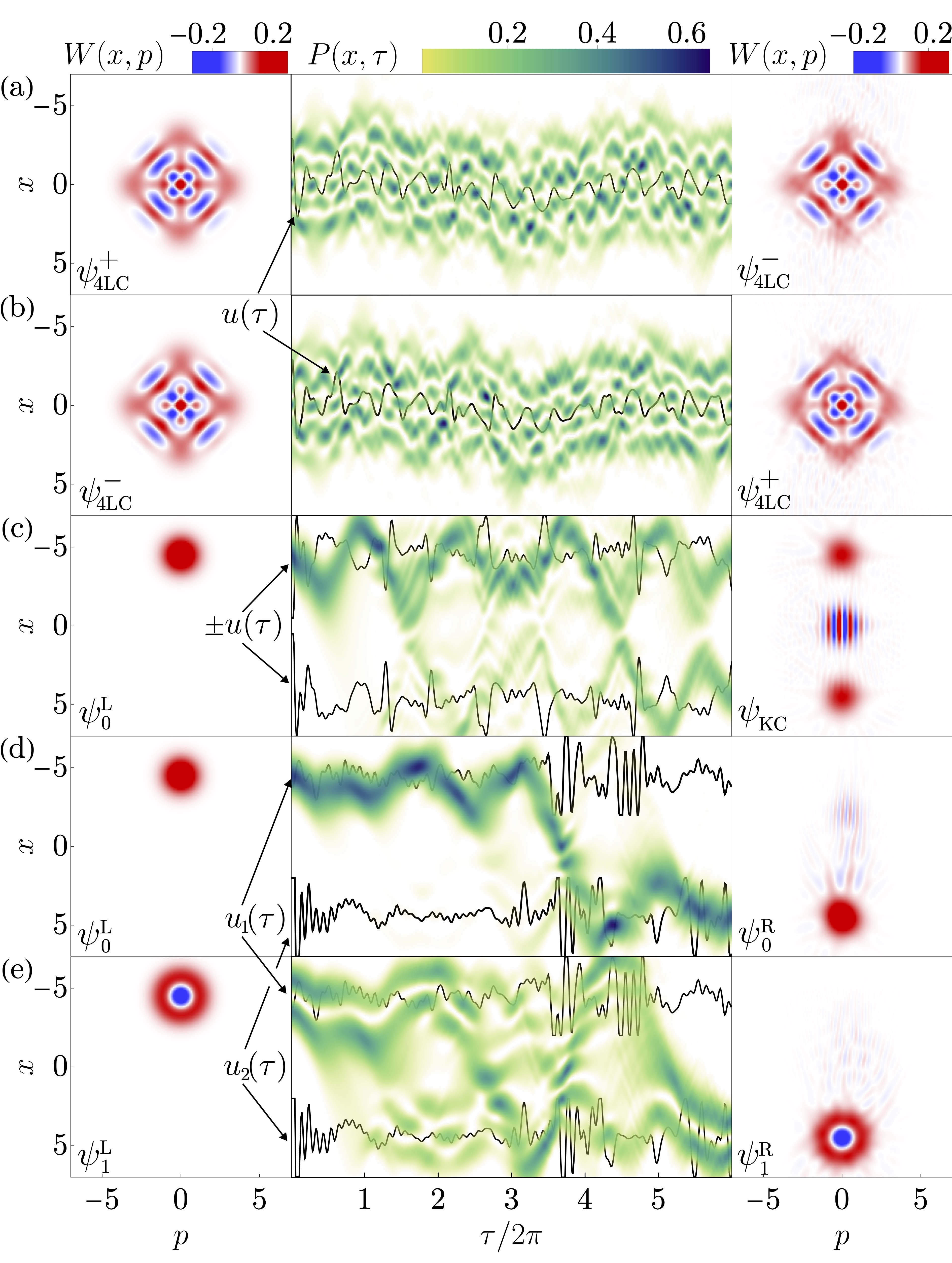
The next type of protocol involves the implementation of a specific unitary within a selected subspace. For simplicity and relevance to several proposals and realizations of bosonic qubits [57, 58, 13, 15, 14, 16, 59, 17], we analyze an example of a two-level subspace. This subspace can be spanned by any two orthogonal states , including two lowest-lying vibrational states and (Fock basis), two mutually displaced GKP states (GKP basis), four-, and two-legged-cat bases. Here, we present a four-legged-cat basis, however, other examples can be found in SM [52]. For the protocol considered, the cost function is the subspace average gate fidelity [60], where , is a projector onto a subspace, is a target unitary, and is a unitary generated through Eq. (1). Again, taking advantage of the optimized position of the potential and additional slight optimized modulation of the depth , we present several examples of unitaries, e.g., or Hadamard operations, for above-mentioned subspaces. In Fig. 2(a,b) we show an exemplary case of four-legged-cat basis and operation performed with a Gaussian potential, where the basis states are given by , respectively [61, 62]. Here, the coherent state reads and are the normalization constants. In this example, we use . Again, the protocol is performed with high fidelity, .
Up to now, we have analyzed quantum dynamics taking place in a single well of a potential landscape. Here, we bring our attention to the nonharmonic potential landscape case that involves two independently controlled potential wells. Such a realization is available for optical lattices, optical tweezers [39, 63, 64, 54, 65], or various circuit quantum electrodynamics setups [66]. First, we address the state preparation and single-particle unitary implementation with two potential wells. We assume that we have two independently controlled wells at our disposal, such that the total potential reads with two independent position control functions, 111Here, we assume that contains only a single well with some characteristic width.. Here, controlling the relative distance between the wells amounts to changing the barrier height, which affects the coupling between the bound states in each of the wells. It can be understood as mode multiplexing [68], accelerated through the optimal control. In Fig. 2(c), we show a balanced cat state preparation utilizing two Gaussian potential wells, , where is the separation between the wells. Note that the presented control is symmetric, , and the instantaneous separation between the wells is constrained in the optimization. The fidelity of the presented protocol yields . The cat states produced in such a manner are pertinent to the fundamental tests of quantum mechanics, especially for massive objects. This protocol, along with a fast optimized transport [42], should allow for a fast macroscopic cat state creation and interferometric protocols.
The double-well potential has also been shown to provide a platform for fault-tolerant quantum computing with so-called Kerr-cats [15]. There, the computational subspace is spanned by superpositions of the ground states of the respective wells, corresponding to the (almost) degenerate ground-state manifold of a full double-well potential, . With optimal control, one can again realize arbitrary unitaries within this subspace (cf. SM [52]). Going further, independent control of two wells can also be utilized to perform a state-preserving transport from one well to the other [see Fig. 2(d,e) for the example of a state of two lowest vibrational levels of the left well transferred to the right one, ].
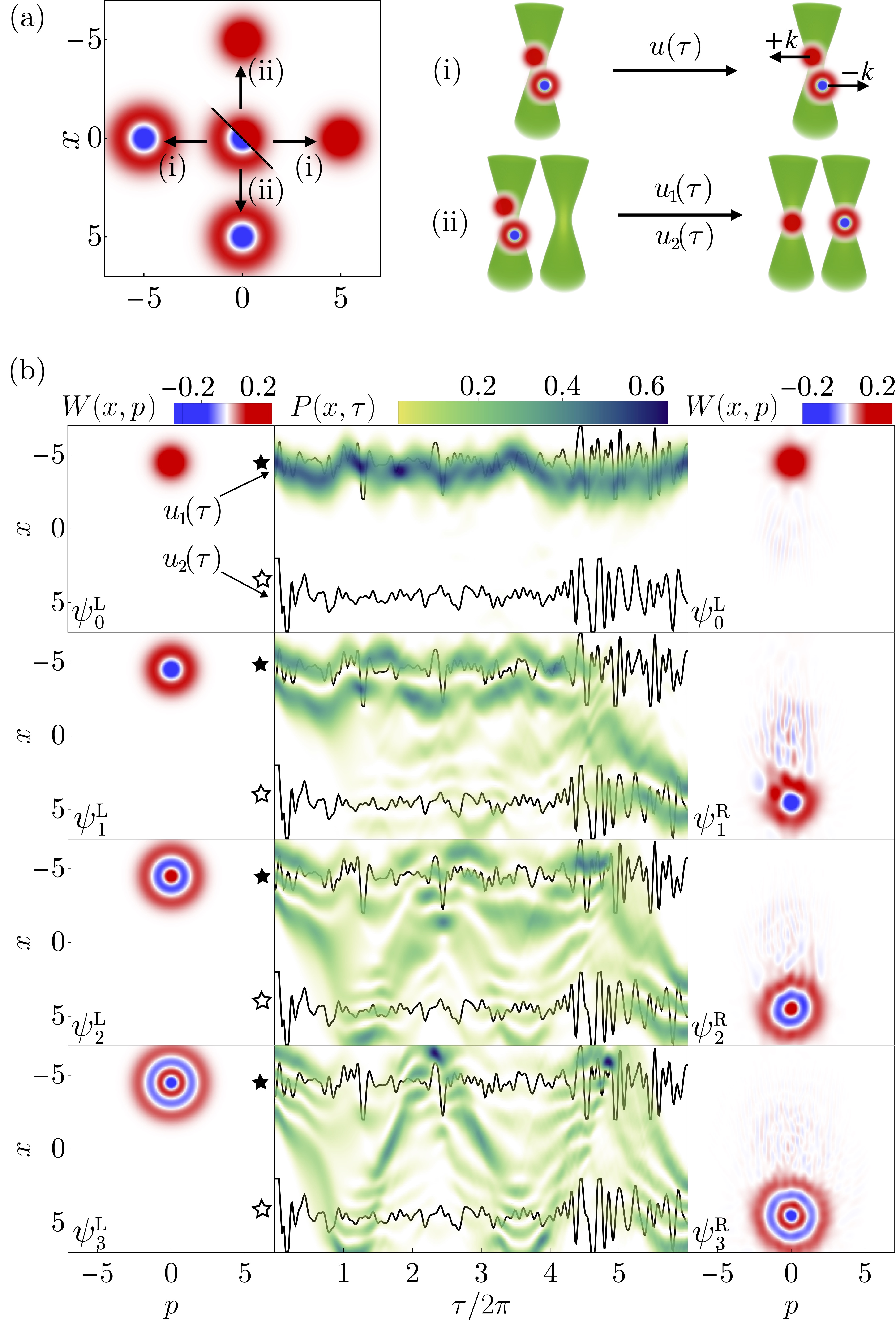
After presenting state preparation and unitary implementation in various nonharmonic potential landscapes, we move on to two protocols that perform single-shot discrimination between two orthogonal states [see Fig. 3(a)], providing an alternative to already existing methods in the considered setups. The first one involves a single nonharmonic well and is performed through imprinting opposite momentum kicks onto each of the states via a potential displacement, , where is chosen such that two phase-imprinted states are nonoverlapping in phase space. After the phase imprinting, a selective measurement takes place, which can be realized in, e.g., optical tweezer setup through the subsequent release of the trap in which time-of-flight evolution reveals spatially separated detection clicks for each of the states [69, 41]. As an example, in Fig. 3(a) are taken to be the two lowest eigenstates of the well. However, different choices can be implemented analogously and we show each of these momentum kick protocols in SM [52]. The second discrimination protocol involves a double-well potential landscape and utilizes spatial separation instead of the momentum one [see Fig. 3(a)]. Initially, the states are fully confined to the left well and their discrimination is realized through a selective stealing protocol—if the state is , then it ends up in the second well after the optimal shaking, while stays in the initial one. Then, large spatial separation between the wells enables selective measurement. Again, other discrimination tasks can also be implemented this way, which we show in SM [52].
These methods performed on low-lying eigenstates of a nonharmonic well can be straightforwardly extended into cooling protocols, similar to algorithmic [36] or evaporative cooling. These protocols involve bringing not only the first excited state but also higher excited states into a second potential well or kicking them out of the well. Fig. 3(b) demonstrates this process for the four lowest states of the well, with the higher three states becoming spatially separated from the ground state and subsequently measured.
After putting forth several protocols, let us now address aspects relevant to their experimental implementation. First, we will analyze the speed at which these protocols can be carried out in the absence of decoherence and which level of nonharmonicity is beneficial. Then, their robustness against decoherence arising from imperfections and coupling to other degrees of freedom will be checked. From now on, we will focus on the state preparation protocol with a single-well Gaussian potential. Concerning the protocol’s speed, a fundamental restriction exists, the quantum speed limit [70], which gives the minimal time that is needed to perform a specific state transfer with a given fidelity threshold. Well-understood for two-level systems driven by static Hamiltonians [70, 71, 72], quantum speed limits have also been analyzed for time-dependent multilevel systems [73, 74], and, specifically, for the ground to the first excited state transfer in one-dimensional Bose-Einstein condensate [46]. We analyze such a case in a Gaussian potential to find a minimum time needed to perform the excitation from the ground to the first excited state, , with some infidelity threshold for different values of nonharmonicity [see Fig. 4(a)]. In the regime of interest, , there is no strong scaling of with the nonharmonicity and achievable fidelity scales exponentially with the protocol time. For the example of an optical tweezer, it implies that, without noise, the deeper the tweezer, the more bound states accessed and the faster the protocol (and hence also requiring more control bandwidth), as . We then analyze the number of excitations averaged throughout the protocol, , as it is relevant for analytical quantum speed limits [72, 75, 76] and proneness to decoherence. Fig. 4(b) shows the results for the Gaussian potential, displaying an increase of the average excitation number with decreasing nonharmonicity, indicating that more nonharmonic potentials are preferred when low excitation is necessitated.
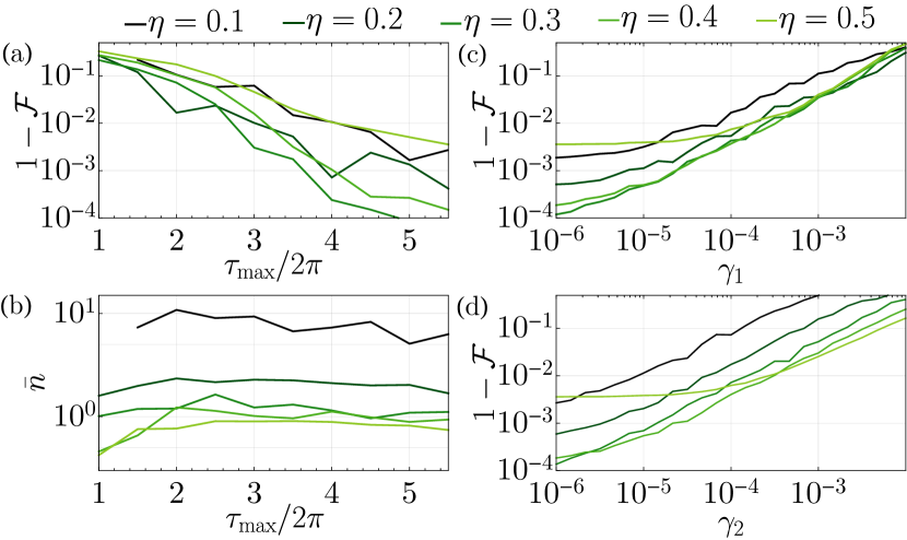
Let us now address the noise robustness of the state preparation protocols. In general, for different experimental realizations, typical sources of error include stochastic vibrations of the potential, low-frequency drifts between experimental runs, imperfections of the control, etc. To model potential vibrations and control imperfections in a single potential well, we employ stochastic fluctuations of the depth and position of the potential, and , where for are dimensionless stochastic Gaussian variables of zero mean and assumed delta-correlated in the relevant time scales, namely . We solve noisy dynamics by averaging over different noise realizations and constructing a Monte Carlo density matrix [77]. In Figs. 4(c,d) we plot the minimal achievable infidelity at a given level of noise for the ground to the first excited state excitation protocol for a single Gaussian potential. While the positional noise affects the protocol comparably for each , the depth noise influences the strongest the least nonharmonic case. By mapping onto pointing and intensity noise in an optical tweezer setup, we find that shallower (more nonharmonic) tweezers outperform the deeper ones—in the presence of a finite amount of noise, to achieve a given infidelity goal, sufficient nonharmonicity is needed, implying also a minimal protocol time (see SM [52]). Presented results can also be applied to the flux-tunable transmon (cosine) case as map onto flux intensity noise to provide necessary noise levels for the experimental realization (cf. SM [52]). As for the low-frequency drifts, one can further optimize the control functions in the presence of varying experimental parameters, a commonly utilized technique [35].
Another experimental challenge might come from coherent coupling to other degrees of freedom. The exemplary case of such a noisy channel occurs in one of the setups we consider and is due to the dimensionality of the realistic optical potential—a three-dimensional tweezer potential is necessarily nonseparable and, depending on the axis of control, axial or radial, a one-dimensional approximation may be less strictly satisfied. Restricting control to only one direction unavoidably leads to excitation in other ones. However, the fidelity loss due to these excitations can be alleviated through additional optimization in fully three-dimensional potential and additional optimized position and depth controls. The additional control then effectively deexcites the coupled degrees of freedom. This optimization can be done via a staged procedure, where the initial guess for a higher-dimensional system comes from a reduced-dimensional control optimization (for details, see SM [52]). Such an optimization procedure can be utilized in setups in which coherent dynamics beyond one-dimensional approximation can be solved. Going beyond the single-well case, note that arbitrary control of double-well systems can also lead to additional sources of noise, including, e.g., relative bias fluctuations.
In conclusion, we have presented a framework that allows the preparation and manipulation of a state of a single continuous-variable degree of freedom and does not necessitate the use of auxiliary nonlinear couplings. The method utilizes optimal control of the intrinsic nonharmonicity present in the effective confining potential, a scenario that is ubiquitous in a plethora of continuous-variable systems, including neutral atoms in optical tweezers and lattices or flux-tunable transmons. We have presented versatile quantum state preparation, implementation of arbitrary unitaries within a selected subspace, quantum discrimination, and cooling protocols that can be realized in such systems. We have shown that these protocols can be performed via both single- and double-well potential landscapes. Moreover, we have analyzed the performance of the state preparation protocols under the effect of position and depth noises. Our proposal is compatible with state-of-the-art technology, such as neutral atoms, circuit quantum electrodynamics, or Bose-Einstein condensates, and might be explored in systems with much smaller nonharmonicities, e.g., ions in Paul traps (typically ) [78, 24] or levitated nanoparticles () [79, 80].
Acknowledgements.
We thank R. G. Cortiñas, N. E. Frattini, S. Muleady, A. M. Rey, and P. Zoller for helpful discussions. The optimization has been implemented with Quantum Optimal Control Suite [35]. The computational results presented here have been achieved in part using the LEO HPC infrastructure of the University of Innsbruck. P.T.G. and O.R.-I. have been supported by the European Union’s Horizon 2020 research and innovation programme under grant agreement No. 863132 (IQLev) and by the European Research Council (ERC) under the grant agreement No. 951234 (Q-Xtreme ERC-2020-SyG). H.P. has been supported through an ERC Starting grant QARA (grant no. 101041435) and the European Union’s Horizon 2020 research and innovation program under Grant Agreement No. 101079862 (PASQuanS2). C.A.R. has been supported by NSF PHY-2317149, NSF QLCI award OMA 2016244, the US Department of Energy, Office of Science, National Quantum Information Science Research Centers, Quantum Systems Accelerator, and the Baur-SPIE Chair at JILA.References
- Zurek [2001] W. H. Zurek, Nature 412, 712 (2001).
- Deléglise et al. [2008] S. Deléglise, I. Dotsenko, C. Sayrin, J. Bernu, M. Brune, J.-M. Raimond, and S. Haroche, Nature 455, 510 (2008).
- Arndt et al. [1999] M. Arndt, O. Nairz, J. Vos-Andreae, C. Keller, G. van der Zouw, and A. Zeilinger, Nature 401, 680 (1999).
- Fein et al. [2019] Y. Y. Fein, P. Geyer, P. Zwick, F. Kiałka, S. Pedalino, M. Mayor, S. Gerlich, and M. Arndt, Nat. Phys. 15, 1242 (2019).
- Bild et al. [2023] M. Bild, M. Fadel, Y. Yang, U. von Lüpke, P. Martin, A. Bruno, and Y. Chu, Science 380, 274 (2023).
- Peters et al. [2001] A. Peters, K. Y. Chung, and S. Chu, Metrologia 38, 25 (2001).
- Graham et al. [2013] P. W. Graham, J. M. Hogan, M. A. Kasevich, and S. Rajendran, Phys. Rev. Lett. 110, 171102 (2013).
- Parker et al. [2018] R. H. Parker, C. Yu, W. Zhong, B. Estey, and H. Müller, Science 360, 191 (2018).
- Margalit et al. [2021] Y. Margalit, O. Dobkowski, Z. Zhou, O. Amit, Y. Japha, S. Moukouri, D. Rohrlich, A. Mazumdar, S. Bose, C. Henkel, and R. Folman, Sci. Adv. 7, eabg2879 (2021).
- Gottesman et al. [2001] D. Gottesman, A. Kitaev, and J. Preskill, Phys. Rev. A 64, 012310 (2001).
- Knill et al. [2001] E. Knill, R. Laflamme, and G. J. Milburn, Nature 409, 46 (2001).
- Heeres et al. [2017] R. W. Heeres, P. Reinhold, N. Ofek, L. Frunzio, L. Jiang, M. H. Devoret, and R. J. Schoelkopf, Nat. Commun. 8, 94 (2017).
- Reinhold et al. [2020] P. Reinhold, S. Rosenblum, W.-L. Ma, L. Frunzio, L. Jiang, and R. J. Schoelkopf, Nat. Phys. 16, 822 (2020).
- Ma et al. [2020] Y. Ma, Y. Xu, X. Mu, W. Cai, L. Hu, W. Wang, X. Pan, H. Wang, Y. P. Song, C.-L. Zou, and L. Sun, Nat. Phys. 16, 827 (2020).
- Grimm et al. [2020] A. Grimm, N. E. Frattini, S. Puri, S. O. Mundhada, S. Touzard, M. Mirrahimi, S. M. Girvin, S. Shankar, and M. H. Devoret, Nature 584, 205 (2020).
- Gertler et al. [2021] J. M. Gertler, B. Baker, J. Li, S. Shirol, J. Koch, and C. Wang, Nature 590, 243 (2021).
- de Neeve et al. [2022] B. de Neeve, T.-L. Nguyen, T. Behrle, and J. P. Home, Nat. Phys. 18, 296 (2022).
- González-Cuadra et al. [2023] D. González-Cuadra, D. Bluvstein, M. Kalinowski, R. Kaubruegger, N. Maskara, P. Naldesi, T. V. Zache, A. M. Kaufman, M. D. Lukin, H. Pichler, B. Vermersch, J. Ye, and P. Zoller, Proc. Natl. Acad. Sci. 120, e2304294120 (2023).
- Cirac et al. [1996] J. I. Cirac, A. S. Parkins, R. Blatt, and P. Zoller, in Advances In Atomic, Molecular, and Optical Physics, Vol. 37, edited by B. Bederson and H. Walther (Academic Press, 1996) pp. 237–296.
- Meekhof et al. [1996] D. M. Meekhof, C. Monroe, B. E. King, W. M. Itano, and D. J. Wineland, Phys. Rev. Lett. 76, 1796 (1996).
- Loredo et al. [2019] J. C. Loredo, C. Antón, B. Reznychenko, P. Hilaire, A. Harouri, C. Millet, H. Ollivier, N. Somaschi, L. De Santis, A. Lemaître, I. Sagnes, L. Lanco, A. Auffèves, O. Krebs, and P. Senellart, Nat. Photonics 13, 803 (2019).
- Trivedi et al. [2020] R. Trivedi, K. A. Fischer, J. Vučković, and K. Müller, Adv. Quantum Technol. 3, 1900007 (2020).
- Jáuregui et al. [2001] R. Jáuregui, N. Poli, G. Roati, and G. Modugno, Phys. Rev. A 64, 033403 (2001).
- Home et al. [2011] J. P. Home, D. Hanneke, J. D. Jost, D. Leibfried, and D. J. Wineland, New J. Phys. 13, 073026 (2011).
- Blais et al. [2021] A. Blais, A. L. Grimsmo, S. M. Girvin, and A. Wallraff, Rev. Mod. Phys. 93, 025005 (2021).
- Gorman et al. [2005] J. Gorman, D. G. Hasko, and D. A. Williams, Phys. Rev. Lett. 95, 090502 (2005).
- Gollub et al. [2006] C. Gollub, U. Troppmann, and R. de Vivie-Riedle, New J. Phys. 8, 48 (2006).
- Koch et al. [2007] J. Koch, T. M. Yu, J. Gambetta, A. A. Houck, D. I. Schuster, J. Majer, A. Blais, M. H. Devoret, S. M. Girvin, and R. J. Schoelkopf, Phys. Rev. A 76, 042319 (2007).
- Schreier et al. [2008] J. A. Schreier, A. A. Houck, J. Koch, D. I. Schuster, B. R. Johnson, J. M. Chow, J. M. Gambetta, J. Majer, L. Frunzio, M. H. Devoret, S. M. Girvin, and R. J. Schoelkopf, Phys. Rev. B 77, 180502 (2008).
- Pistolesi et al. [2021] F. Pistolesi, A. N. Cleland, and A. Bachtold, Phys. Rev. X 11, 031027 (2021).
- Leghtas et al. [2013a] Z. Leghtas, G. Kirchmair, B. Vlastakis, M. H. Devoret, R. J. Schoelkopf, and M. Mirrahimi, Phys. Rev. A 87, 042315 (2013a).
- Zheng et al. [2021] Y. Zheng, O. Hahn, P. Stadler, P. Holmvall, F. Quijandría, A. Ferraro, and G. Ferrini, PRX Quantum 2, 010327 (2021).
- Glaser et al. [2015] S. J. Glaser, U. Boscain, T. Calarco, C. P. Koch, W. Köckenberger, R. Kosloff, I. Kuprov, B. Luy, S. Schirmer, T. Schulte-Herbrüggen, D. Sugny, and F. K. Wilhelm, Eur. Phys. J. D 69, 279 (2015).
- Koch et al. [2022] C. P. Koch, U. Boscain, T. Calarco, G. Dirr, S. Filipp, S. J. Glaser, R. Kosloff, S. Montangero, T. Schulte-Herbrüggen, D. Sugny, and F. K. Wilhelm, EPJ Quantum Technol. 9, 1 (2022).
- Rossignolo et al. [2023] M. Rossignolo, T. Reisser, A. Marshall, P. Rembold, A. Pagano, P. J. Vetter, R. S. Said, M. M. Müller, F. Motzoi, T. Calarco, F. Jelezko, and S. Montangero, Comput. Phys. Commun. 291, 108782 (2023).
- Popp et al. [2006] M. Popp, J.-J. Garcia-Ripoll, K. G. H. Vollbrecht, and J. I. Cirac, New J. Phys. 8, 164 (2006).
- Serwane [2011] F. Serwane, Deterministic Preparation of a Tunable Few-Fermion System, Ph.D. thesis, Ruprecht-Karls-Universität Heidelberg (2011).
- Serwane et al. [2011] F. Serwane, G. Zürn, T. Lompe, T. B. Ottenstein, A. N. Wenz, and S. Jochim, Science 332, 336 (2011).
- Kaufman et al. [2014] A. M. Kaufman, B. J. Lester, C. M. Reynolds, M. L. Wall, M. Foss-Feig, K. R. A. Hazzard, A. M. Rey, and C. A. Regal, Science 345, 306 (2014).
- Kaufman et al. [2015] A. M. Kaufman, B. J. Lester, M. Foss-Feig, M. L. Wall, A. M. Rey, and C. A. Regal, Nature 527, 208 (2015).
- Brown et al. [2023] M. O. Brown, S. R. Muleady, W. J. Dworschack, R. J. Lewis-Swan, A. M. Rey, O. Romero-Isart, and C. A. Regal, Nat. Phys. 19, 569 (2023).
- Lam et al. [2021] M. R. Lam, N. Peter, T. Groh, W. Alt, C. Robens, D. Meschede, A. Negretti, S. Montangero, T. Calarco, and A. Alberti, Phys. Rev. X 11, 011035 (2021).
- Hutchings et al. [2017] M. D. Hutchings, J. B. Hertzberg, Y. Liu, N. T. Bronn, G. A. Keefe, M. Brink, J. M. Chow, and B. L. T. Plourde, Phys. Rev. Appl. 8, 044003 (2017).
- Bücker et al. [2011] R. Bücker, J. Grond, S. Manz, T. Berrada, T. Betz, C. Koller, U. Hohenester, T. Schumm, A. Perrin, and J. Schmiedmayer, Nat. Phys. 7, 608 (2011).
- Bücker et al. [2013] R. Bücker, T. Berrada, S. van Frank, J.-F. Schaff, T. Schumm, J. Schmiedmayer, G. Jäger, J. Grond, and U. Hohenester, J. Phys. B: At. Mol. Opt. Phys. 46, 104012 (2013).
- van Frank et al. [2016] S. van Frank, M. Bonneau, J. Schmiedmayer, S. Hild, C. Gross, M. Cheneau, I. Bloch, T. Pichler, A. Negretti, T. Calarco, and S. Montangero, Sci. Rep. 6, 34187 (2016).
- Xu et al. [2022] S. Xu, J. Schmiedmayer, and B. C. Sanders, Phys. Rev. Res. 4, 023071 (2022).
- Calarco et al. [2004] T. Calarco, U. Dorner, P. S. Julienne, C. J. Williams, and P. Zoller, Phys. Rev. A 70, 012306 (2004).
- Dorner et al. [2005] U. Dorner, T. Calarco, P. Zoller, A. Browaeys, and P. Grangier, J. Opt. B: Quantum Semiclass. Opt. 7, S341 (2005).
- Sterk et al. [2022] J. D. Sterk, H. Coakley, J. Goldberg, V. Hietala, J. Lechtenberg, H. McGuinness, D. McMurtrey, L. P. Parazzoli, J. Van Der Wall, and D. Stick, npj Quantum Inf. 8, 1 (2022).
- Puri et al. [2017] S. Puri, S. Boutin, and A. Blais, npj Quantum Inf. 3, 1 (2017).
- [52] See Supplemental Material for the mappings onto physical systems, examples of state preparation protocols, single- and double-well two-level unitary implementations, momentum kick protocols, selective stealing protocols, noise mappings and analysis, and state preparation in two and three dimensions.
- Dykman [2012] M. Dykman, ed., Fluctuating Nonlinear Oscillators: From Nanomechanics to Quantum Superconducting Circuits (Oxford University Press, Oxford, United Kingdom, 2012).
- Kaufman and Ni [2021] A. M. Kaufman and K.-K. Ni, Nat. Phys. 17, 1324 (2021).
- Rol et al. [2019] M. A. Rol, F. Battistel, F. K. Malinowski, C. C. Bultink, B. M. Tarasinski, R. Vollmer, N. Haider, N. Muthusubramanian, A. Bruno, B. M. Terhal, and L. DiCarlo, Phys. Rev. Lett. 123, 120502 (2019).
- Müller et al. [2022] M. M. Müller, R. S. Said, F. Jelezko, T. Calarco, and S. Montangero, Rep. Prog. Phys. 85, 076001 (2022).
- Ma et al. [2021] W.-L. Ma, S. Puri, R. J. Schoelkopf, M. H. Devoret, S. M. Girvin, and L. Jiang, Sci. Bull. 66, 1789 (2021).
- Rosenblum et al. [2018] S. Rosenblum, P. Reinhold, M. Mirrahimi, L. Jiang, L. Frunzio, and R. J. Schoelkopf, Science 361, 266 (2018).
- Flühmann et al. [2019] C. Flühmann, T. L. Nguyen, M. Marinelli, V. Negnevitsky, K. Mehta, and J. P. Home, Nature 566, 513 (2019).
- Pedersen et al. [2007] L. H. Pedersen, N. M. Møller, and K. Mølmer, Phys. Lett. A 367, 47 (2007).
- Leghtas et al. [2013b] Z. Leghtas, G. Kirchmair, B. Vlastakis, R. J. Schoelkopf, M. H. Devoret, and M. Mirrahimi, Phys. Rev. Lett. 111, 120501 (2013b).
- Mirrahimi et al. [2014] M. Mirrahimi, Z. Leghtas, V. V. Albert, S. Touzard, R. J. Schoelkopf, L. Jiang, and M. H. Devoret, New J. Phys. 16, 045014 (2014).
- Murmann et al. [2015] S. Murmann, A. Bergschneider, V. M. Klinkhamer, G. Zürn, T. Lompe, and S. Jochim, Phys. Rev. Lett. 114, 080402 (2015).
- Islam et al. [2015] R. Islam, R. Ma, P. M. Preiss, M. Eric Tai, A. Lukin, M. Rispoli, and M. Greiner, Nature 528, 77 (2015).
- Yan et al. [2022] Z. Z. Yan, B. M. Spar, M. L. Prichard, S. Chi, H.-T. Wei, E. Ibarra-García-Padilla, K. R. A. Hazzard, and W. S. Bakr, Phys. Rev. Lett. 129, 123201 (2022).
- Frattini et al. [2022] N. E. Frattini, R. G. Cortiñas, J. Venkatraman, X. Xiao, Q. Su, C. U. Lei, B. J. Chapman, V. R. Joshi, S. M. Girvin, R. J. Schoelkopf, S. Puri, and M. H. Devoret, arXiv.2209.03934 (2022).
- Note [1] Here, we assume that contains only a single well with some characteristic width.
- Martínez-Garaot et al. [2013] S. Martínez-Garaot, E. Torrontegui, X. Chen, M. Modugno, D. Guéry-Odelin, S.-Y. Tseng, and J. G. Muga, Phys. Rev. Lett. 111, 213001 (2013).
- Fuhrmanek et al. [2010] A. Fuhrmanek, A. M. Lance, C. Tuchendler, P. Grangier, Y. R. P. Sortais, and A. Browaeys, New J. Phys. 12, 053028 (2010).
- Deffner and Campbell [2017] S. Deffner and S. Campbell, J. Phys. A: Math. Theor. 50, 453001 (2017).
- Mandelstam and Tamm [1945] L. Mandelstam and I. Tamm, J. Phys. USSR 9, 249 (1945).
- Margolus and Levitin [1998] N. Margolus and L. B. Levitin, Physica D 120, 188 (1998).
- Anandan and Aharonov [1990] J. Anandan and Y. Aharonov, Phys. Rev. Lett. 65, 1697 (1990).
- Deffner and Lutz [2013] S. Deffner and E. Lutz, J. Phys. A: Math. Theor. 46, 335302 (2013).
- Chen and Muga [2010] X. Chen and J. G. Muga, Phys. Rev. A 82, 053403 (2010).
- Ness et al. [2021] G. Ness, M. R. Lam, W. Alt, D. Meschede, Y. Sagi, and A. Alberti, Sci. Adv. 7, eabj9119 (2021).
- Mølmer et al. [1993] K. Mølmer, Y. Castin, and J. Dalibard, J. Opt. Soc. Am. B 10, 524 (1993).
- Leibfried et al. [2003] D. Leibfried, R. Blatt, C. Monroe, and D. Wineland, Rev. Mod. Phys. 75, 281 (2003).
- Gonzalez-Ballestero et al. [2021] C. Gonzalez-Ballestero, M. Aspelmeyer, L. Novotny, R. Quidant, and O. Romero-Isart, Science 374, eabg3027 (2021).
- Roda-Llordes et al. [2023] M. Roda-Llordes, A. Riera-Campeny, D. Candoli, P. T. Grochowski, and O. Romero-Isart, arXiv.2303.07959 (2023).
See pages ,1,,2,,3,,4,,5,,6,,7,,8,,9 of supplemental_material.pdf