All invariant gluon OPEs on the celestial sphere
Abstract
algebra is an infinite dimensional Lie algebra which is known to be the symmetry algebra of some gauge theories. It is a "coloured version" of the . In this paper we write down all possible invariant (celestial) OPEs between two positive helicity outgoing gluons and also find the Knizhnik-Zamolodchikov type null states for these theories. Our analysis hints at the existence of an infinite number of invariant gauge theories which include the (tree-level) MHV-sector and the self-dual Yang-Mills theory.
1 Introduction
S-matrix is an important observable in any quantum field theory in asymptotically flat spacetime. In fact in quantum theory of gravity S-matrix is argued to be the only observable. Therefore any holographic dual theory has to compute the S-matrix elements or scattering amplitudes in the bulk. Celestial holography is an attempt in this direction Strominger:2017zoo ; Pasterski:2021rjz ; Donnay:2023mrd . The realization that the soft theorems of gauge theories and gravity are the Ward identities for different asymptotic symmetries Strominger:2013lka ; Strominger:2013jfa ; He ; Strominger:2014pwa ; Campiglia:2016jdj ; Kapec:2016jld ; Kapec:2014opa ; Banerjee:2020vnt ; He:2017fsb ; Banerjee:2022wht ; Donnay:2021wrk ; Donnay:2020guq ; Stieberger:2018onx ; Banerjee:2020kaa ; Banerjee:2020zlg ; Banerjee:2021cly ; Gupta:2021cwo ; Guevara:2021abz ; Strominger:2021mtt ; Himwich:2021dau ; Melton:2022fsf ; Adamo:2021lrv ; Costello:2022wso ; Costello:2022upu ; Costello:2023vyy ; Garner:2023izn ; Stieberger:2022zyk ; Stieberger:2023fju ; Magnea:2021fvy ; Gonzalez:2021dxw has led to important insights into the study of scattering amplitudes rewritten as correlators of a conformal field theory on the 2D celstial sphere. This CFT is commonly known as the celestial conformal field theory (CCFT). The map from scattering amplitudes to the correlators of CCFT is done via the Mellin transformation. Usually scattering amplitudes are written in momentum basis. The job of Mellin transformation is to change the momentum eigenbasis into boost eigenbasis Pasterski:2016qvg ; Pasterski:2017kqt ; Banerjee:2018gce ; Banerjee:2019prz . The isomorphism between the global conformal group in 2D and the Lorentz group in 4D is at the heart of this basis change.
Operator Product Expansion (OPE) in CCFT correspond to the collinear limit in the bulk and it plays a very important role in the study of the dual theory Fan:2019emx ; Banerjee:2020zlg ; Banerjee:2021cly ; Guevara:2021abz ; Himwich:2021dau ; Costello:2022upu ; Banerjee:2023zip ; Ebert:2020nqf ; Adamo:2022wjo ; Ren:2023trv ; Hu:2021lrx ; Fan:2022vbz ; Fan:2022kpp ; Bhardwaj:2022anh ; Krishna:2023ukw ; Hu:2022bpa ; Pate:2019lpp ; Atanasov:2021cje ; Banerjee:2023jne ; Banerjee:2023rni ; Ball:2023qim . In a previous paper Banerjee:2023zip , we have studied the invariant OPEs in theories of gravity. Our analysis showed that there are an infinite number of theories on the celestial sphere which are invariant. By deriving the OPE from graviton scattering amplitudes we have explicitly shown in Banerjee:2023jne that the self dual gravity is one example of this infinite family.
In this paper we perform a similar analysis for gluons. In the case of gluons the infinite symmetry algebra is know as the algebra Guevara:2021abz ; Strominger:2021mtt . We write down all possible invariant OPE structures between two positive helicity outgoing gluons. We find that there is a (discrete) infinite number of such structures and presumably, each one of them corresponds to a invariant theory of gluons in the bulk. However, a more explicit Lagrangian description of these theories are not known to us.
There is an important difference between the analyses of and -invariant theories, which we want to point out. algebra does not contain the Poincare generators. Therefore the consistent OPEs need not be Poincare invariant. However in this paper we make sure that all the OPEs are (conformal) Lorentz invariant and this plays an important role. This is along the line of Fan:2022vbz ; Fan:2022kpp ; Banerjee:2023rni ; Casali:2022fro .
We start with a brief review of the soft gluon symmetry algebra known as the algebra in section 2. In section 3, the general structure of the OPE between two positive helicity outgoing gluons on the celestial sphere has been discussed. We have argued, how the null states of the MHV-sector can be used to write down the general OPE. In section 4, we have written down the null states that appear at of the gluon-gluon OPE in the MHV-sector. These are not the complete set of null states that the MHV sector has at . There are more of them. We talk about them later in section 8, where we have discussed the Knizhnik-Zamolodchikov (KZ)-type null states. Section 5 explicitly shows how to organise the OPE at every order. For simplicity we focus on the terms in the OPE. We have also discussed the transformation properties of MHV-null states under the algebra in this section, which are required to organise the OPE. Section 6 shows the invariance of the OPE under algebra. In section 7, we have argued, how an infinite number theories can exist on the celestial sphere. We conclude the paper with the discussion of the results found in this paper and some future directions in section 8.1.
2 The S algebra
We start by describing the soft symmetry algebra which follows from the universal singular terms in the OPE between two positive helicity outgoing gluons Guevara:2021abz ; Strominger:2021mtt . Let denote a positive helicity outgoing gluon conformal primary operator of dimension at the point on the celestial sphere. The universal singular terms in the OPE are given by
| (1) |
The interesting fact about these singular OPE coefficients is that it allows us to define an infinite tower of conformally soft Donnay:2018neh ; Pate:2019mfs ; Fan:2019emx ; Nandan:2019jas ; Adamo:2019ipt ; Puhm:2019zbl ; Guevara:2019ypd gluons Guevara:2021abz ; Strominger:2021mtt by
| (2) |
Now it follows from the structure of the OPE (1) that one can introduce the following truncated mode expansion
| (3) |
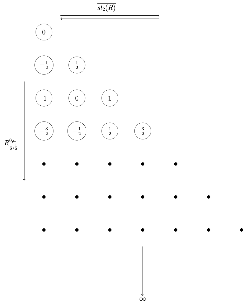
where the expansion coefficients are the conserved holomorphic currents. For fixed values of and there are such currents and they transform in the dimensional representation of the .
The holomorphic currents can be further mode expanded as
| (4) |
The algebra of these modes can be obtained from the singular terms (1) of the OPE and is given by Guevara:2021abz ,
| (5) |
Now one can define the following generators Strominger:2021mtt
| (6) |
in terms of which the algebra (5) simplifies to
| (7) |
This infinite dimensional algebra of the conformally soft gluons, known as the algebra, plays a central role in this paper.111In this paper we write the OPE in terms of of the descendants of the algebra (5). However, we will continue to refer to (5) as the algebra.
In this paper we want to classify all possible OPEs between two positive helicity outgoing gluons which are invariant under the algebra. The strategy we adopt here is similar to that in the gravity case Banerjee:2023zip but the details are very different. For example, in the gravity case the soft symmetry algebra which is isomorphic to the contains all four global space-time translations. But, this is not the case for the algebra and so there are invariant theories which are not space-time translationally invariant Fan:2022vbz ; Fan:2022kpp ; Banerjee:2023rni ; Casali:2022fro . However, we preserve Lorentz invariance because it translates into conformal invariance on the celestial sphere and the structure of the algebra depends on that.
3 General structure of the OPE Between two positive helicity outgoing gluons
We can write the general structure of the OPE between two positive helicity gluons invariant under the algebra as
| (8) |
where in the second line we have now added the algebra descendants of a positive helicity gluon. The sum over could be finite or infinite depending on the theory. Our goal is to determine the descendants and the OPE coefficients in a general -invariant theory.
In the gravity case Banerjee:2023zip we found that any -invariant OPE can be written in terms of the MHV OPE and the MHV null states. We have also checked by detailed calculation that this structure holds in the self-dual gravity theory Banerjee:2023jne which is invariant. The same reasoning also goes through for the algebra and gluons. We summarize the argument below.
Since the algebra is universal, i.e the same 222For example, this is not true in the conventional CFTs because different CFTs have different Virasoro central charges and so different conformal symmetry algebras. algebra holds in any invariant theory, it is reasonable to assume that there is a Master OPE which holds in all invariant theories. Let us now consider the gluon-gluon OPE in the (tree-level) MHV sector of the pure YM theory. Since the MHV sector is invariant the Master OPE, when inserted in a MHV gluon scattering amplitude, should reproduce the known MHV sector OPE. Therefore one can write
| (9) |
where should vanish inside an MHV scattering amplitude. This is possible only if is a linear combination of MHV null states. Now since the MHV-sector OPE already contains the universal singular terms (1) of the gluon-gluon OPE, consists only of non-singular terms. So we can write,
| (10) |
where are the MHV null states. So when "Any Theory" is taken to be the MHV sector, vanishes and we get back the MHV sector OPE by construction.
We now describe the MHV null states which are of interest to us. In this paper we apply this general procedure to write down the OPE at .
4 Null states in the MHV sector
The general null state at order is given by 333These null states can be obtained by taking soft limits of the gluon-gluon MHV OPE Banerjee:2020vnt . The relevant terms in the gluon-gluon OPE in the MHV sector which gives rise to these null states are given in (23).
| (11) |
Here we have ignored the index and have simply written instead of for the order MHV null states.
Now it turns out that the following basis of null states
| (12) |
is more convenient because they transform nicely under the -algebra. We will discuss their transformation law in the next section.
We conclude this section by defining the antisymmetric part of the null states as
| (13) |
5 Organizing the OPE at every order
Since the MHV sector is invariant the MHV null states must form a representation of the algebra. In other words every generator of the algebra must map any MHV null state to another MHV null state. Our analysis shows that this representation is reducible and different invariant theories correspond to different irreducible components of this representation. So our first job is to study the action of the algebra generators on the MHV null states. This is facilitated by the following observation.
We have discussed in Section 2 that the algebra is generated by an infinite number of holomorphic soft currents 444Here is the antiholomorphic weight of the current. where is the dimension of the soft operator and . For a fixed , the soft currents transform in a dimensional representation of the 555Note that we are assuming the theory to be (conformal) Lorentz invariant.. This can be seen from the following commutation relations:
| (14) |
Now let us consider the currents with the lowest weights. Starting from all the currents in this family can be obtained by applying the global subleading soft gluon operator . This can be seen from the the following commutation relations
| (15) |
Equations (14) and (15) show that we can write any generator of the algebra as a sum of products of the generators . Therefore in order to study the action of the algebra generators on the MHV null states we just need to focus on these finite number of generators.
5.1 Transformation properties of the null states under algebra
Using the action of different generators of algebra on the gluon primary operators and the commutation relations (14) it is easy to show that
| (16) |
Thus (12) implies that
| (17) |
Therefore the null states are primaries.
5.2 Transformation properties of the null states under the leading soft gluon current algebra
One can easily check that under the leading soft gluon current algebra, the null states (12) transform as
| (18) |
Therefore the null states are the leading soft gluon current algebra primaries.
5.3 Transformation properties of the null states under subleading soft gluon operator
This is perhaps the most important transformation property because it mixes the null states with different values. The action of on is given by,
| (19) |
We have used (37) to derive the above equation.
Now let us consider the set of null states:
| (20) |
From (19) we can see that if we set
| (21) |
then the set (20) is closed under the action of . Moreover it follows from (19) that the infinite set of equations (21) is also invariant under the action of because the index mixes only with . Therefore the truncation (21) is algebra invariant and we can get an invariant OPE if we keep only the finite set (20). Let us emphasize that the integer is in no way restricted by the invariance.
6 OPE and its invariance under the algebra
Let us now consider the terms in the OPE when we keep only the finite set of MHV null states (20). In particular, we show that the terms in the OPE with the following coefficients are -invariant:
| (22) |
where is given by Banerjee:2020vnt ; Ebert:2020nqf
| (23) |
Let us first apply on the OPE (22). After some straightforward algebra we get,
| (24) |
Now, we have argued in the previous section that if the OPE of a invariant theory truncates at , then will be a null state of that theory. Thus, we can set the RHS of (24) to 0 and hence (22) is invariant under the action of . Using (18), one can also verify that, (22) is invariant under the actions of .
In Banerjee:2020vnt , it was shown that the OPE in the MHV-sector is invariant under the action of . We can also see from (16) that the null states are annihilated by . Thus, the OPE (22) is also invariant under . Hence we conclude that the truncated OPE (22) is invariant under the algebra.
7 Infinite family of invariant theories
In section (5.3) we have shown that the following set of equations
| (25) |
are invariant. Thus at we can truncate the OPE (10) at an arbitrary in an -invariant way. That is to say -invariance does not fix the value of the integer . Hence we can get a discrete infinite family of -invariant OPEs for different choices of the integer . Each of these consistent OPEs correspond to a invariant theory of gluons. But, at present we do not know the Lagrangian description of these theories except perhaps the self-dual Yang-Mills theory.
8 Knizhnik-Zamolodchikov type null states
Knizhnik-Zamolodchikov (KZ) type null states contain descendants of the holomorphic translation generator on the celestial sphere. They can be obtained algebraically by determining the relevant primary descendant but in our case we can bypass this tedious procedure if we use the OPE commutativity
| (26) |
The reason behind this is that the terms of the OPE, as written in (22), are not manifestly symmetric under the exchange (26). Therefore OPE commutativity imposes non-trivial constraints on the OPE coefficients and one such constraint is essentially the KZ equation. The process can be further simplified if make the operator leading soft by taking the limit . Now a straightforward calculation gives the KZ type null state
| (27) |
where
| (28) |
is the KZ type null state in the MHV-sector Banerjee:2020vnt and is the antisymmetric part of the null state defined in (13). We have also used the identity in deriving the KZ type null state equation (27).
Another null state equation involving the descendant can be obtained from (26) in a similar way by taking the subleading conformal soft limit . It is given by
| (29) |
Now multiplying equation (27) by and then subtracting it from (29) we get the following (current algebra) null state
| (30) |
One can continue this procedure and get other current algebra null states by taking conformal soft limits . We can denote them by . However, it can be shown that after a finite iteration this procedure stops due to the truncation (21).
8.1 S invariance of the KZ type null state
In this section we show that the KZ type null state (27) is -invariant.
First of all, the states , and as a result , are annihilated by . Therefore the state is a primary of because the KZ type null state (28) in the MHV-sector is annihilated Banerjee:2020vnt by .
Similarly, one can show after some algebra that the following relation holds
| (31) |
where
| (32) |
Now we know that, in a theory in which the OPE truncates at , i.e, (21) holds, both and are null states. Thus we can set them to 0 and get,
| (33) |
We show in Appendix (C) that the second and the third terms on the RHS of (33) are actually zero. Taking this into account we get
| (34) |
Thus we see that maps the KZ type null state to linear combination of other null states in the theory. Hence, the null state equation
| (35) |
is invariant.
9 Acknowledgement
SB would like to thank the participants of the Kickoff Workshop for the Simons Collaboration on Celestial Holography for helpful comments. The work of SB is partially supported by the Swarnajayanti Fellowship (File No- SB/SJF/2021-22/14) of the Department of Science and Technology and SERB, India. The work of PP is supported by an IOE endowed Postdoctoral position at IISc, Bengaluru, India. SP is supported by the INSA Senior scientist position at NISER, Bhubaneswar through the Grant number INSA/SP/SS/2023.
Appendix A algebra primaries
In this Appendix, we write down the conditions on the primary operators that follow from the OPE between two positive helicity outgoing gluon primaries (1). They are obtained by taking different soft limits in (1) and comparing both the sides of the OPE:
| (36) |
where . These conditions have been used in writing down the transformation properties of the MHV null states. For more details of how to obtain these conditions one can check Appendix F of Banerjee:2023jne . The analyses there was done for primaries, but the methodology is same for algebra also.
Appendix B Transformation properties of the -null states under the leading soft gluon operator and the subleading soft gluon operator
Appendix C Proof that the KZ-type null states are closed under the action of
We write the second and third term in (33) as,
| (38) |
The above equation can be decomposed into symmetric and antisymmetric part in the following way,
| (39) |
where
| (40) |
Now, using the Jacobi identity
| (41) |
one can show that
| (42) |
We now simplify the symmetric part (40) and get,
| (43) |
The leading and subleading soft limits of (26) and some straightforward algebra then gives,
| (44) |
Hence we conclude that,
| (45) |
References
- (1) S. Banerjee, H. Kulkarni and P. Paul, “An infinite family of w1+∞ invariant theories on the celestial sphere,” JHEP 05 (2023), 063 doi:10.1007/JHEP05(2023)063 [arXiv:2301.13225 [hep-th]].
- (2) A. Strominger, “Lectures on the Infrared Structure of Gravity and Gauge Theory,” [arXiv:1703.05448 [hep-th]].
- (3) S. Pasterski, “Lectures on celestial amplitudes,” Eur. Phys. J. C 81, no.12, 1062 (2021) doi:10.1140/epjc/s10052-021-09846-7 [arXiv:2108.04801 [hep-th]]
- (4) L. Donnay, “Celestial holography: An asymptotic symmetry perspective,” [arXiv:2310.12922 [hep-th]].
- (5) S. Pasterski, S. H. Shao and A. Strominger, “Flat Space Amplitudes and Conformal Symmetry of the Celestial Sphere,” Phys. Rev. D 96, no. 6, 065026 (2017) doi:10.1103/PhysRevD.96.065026 [arXiv:1701.00049 [hep-th]].
- (6) S. Pasterski and S. H. Shao, “Conformal basis for flat space amplitudes,” Phys. Rev. D 96, no. 6, 065022 (2017) doi:10.1103/PhysRevD.96.065022 [arXiv:1705.01027 [hep-th]].
- (7) S. Banerjee, “Null Infinity and Unitary Representation of The Poincare Group,” JHEP 1901, 205 (2019) doi:10.1007/JHEP01(2019)205 [arXiv:1801.10171 [hep-th]].
- (8) S. Banerjee, S. Ghosh, P. Pandey and A. P. Saha, “Modified celestial amplitude in Einstein gravity,” JHEP 03 (2020), 125 doi:10.1007/JHEP03(2020)125 [arXiv:1909.03075 [hep-th]].
- (9) W. Fan, A. Fotopoulos and T. R. Taylor, “Soft Limits of Yang-Mills Amplitudes and Conformal Correlators,” JHEP 1905, 121 (2019) doi:10.1007/JHEP05(2019)121 [arXiv:1903.01676 [hep-th]].
- (10) M. Pate, A. M. Raclariu, A. Strominger and E. Y. Yuan, “Celestial operator products of gluons and gravitons,” Rev. Math. Phys. 33 (2021) no.09, 2140003 doi:10.1142/S0129055X21400031 [arXiv:1910.07424 [hep-th]].
- (11) A. Strominger, “Asymptotic Symmetries of Yang-Mills Theory,” JHEP 1407, 151 (2014) doi:10.1007/JHEP07(2014)151 [arXiv:1308.0589 [hep-th]].
- (12) A. Strominger, “On BMS Invariance of Gravitational Scattering,” JHEP 1407, 152 (2014) doi:10.1007/JHEP07(2014)152 [arXiv:1312.2229 [hep-th]].
- (13) T. He, V. Lysov, P. Mitra and A. Strominger, “BMS supertranslations and Weinberg’s soft graviton theorem,” JHEP 1505, 151 (2015) doi:10.1007/JHEP05(2015)151 [arXiv:1401.7026 [hep-th]].
- (14) A. Strominger and A. Zhiboedov, “Gravitational Memory, BMS Supertranslations and Soft Theorems,” JHEP 1601, 086 (2016) doi:10.1007/JHEP01(2016)086 [arXiv:1411.5745 [hep-th]].
- (15) M. Campiglia and A. Laddha, “Sub-subleading soft gravitons: New symmetries of quantum gravity?,” Phys. Lett. B 764 (2017), 218-221 doi:10.1016/j.physletb.2016.11.046 [arXiv:1605.09094 [gr-qc]].
- (16) D. Kapec, P. Mitra, A. M. Raclariu and A. Strominger, “2D Stress Tensor for 4D Gravity,” Phys. Rev. Lett. 119, no. 12, 121601 (2017) doi:10.1103/PhysRevLett.119.121601 [arXiv:1609.00282 [hep-th]].
- (17) D. Kapec, V. Lysov, S. Pasterski and A. Strominger, “Semiclassical Virasoro symmetry of the quantum gravity -matrix,” JHEP 1408, 058 (2014) doi:10.1007/JHEP08(2014)058 [arXiv:1406.3312 [hep-th]].
- (18) T. He, D. Kapec, A. M. Raclariu and A. Strominger, “Loop-Corrected Virasoro Symmetry of 4D Quantum Gravity,” JHEP 1708, 050 (2017) doi:10.1007/JHEP08(2017)050 [arXiv:1701.00496 [hep-th]].
- (19) S. Banerjee and S. Pasterski, “Revisiting the shadow stress tensor in celestial CFT,” JHEP 04 (2023), 118 doi:10.1007/JHEP04(2023)118 [arXiv:2212.00257 [hep-th]].
- (20) S. Banerjee, S. Ghosh and R. Gonzo, “BMS symmetry of celestial OPE,” JHEP 04, 130 (2020) doi:10.1007/JHEP04(2020)130 [arXiv:2002.00975 [hep-th]].
- (21) S. Banerjee, S. Ghosh and P. Paul, “MHV graviton scattering amplitudes and current algebra on the celestial sphere,” JHEP 02 (2021), 176 doi:10.1007/JHEP02(2021)176 [arXiv:2008.04330 [hep-th]].
- (22) S. Banerjee and S. Ghosh, “MHV gluon scattering amplitudes from celestial current algebras,” JHEP 10 (2021), 111 doi:10.1007/JHEP10(2021)111 [arXiv:2011.00017 [hep-th]].
- (23) N. Gupta, P. Paul and N. V. Suryanarayana, “ Symmetry of Gravity,” Phys. Rev. D 108 (2023) no.8, 086029 doi:10.1103/PhysRevD.108.086029 [arXiv:2109.06857 [hep-th]].
- (24) A. Guevara, E. Himwich, M. Pate and A. Strominger, “Holographic symmetry algebras for gauge theory and gravity,” JHEP 11 (2021), 152 doi:10.1007/JHEP11(2021)152 [arXiv:2103.03961 [hep-th]].
- (25) A. Strominger, “ Algebra and the Celestial Sphere: Infinite Towers of Soft Graviton, Photon, and Gluon Symmetries,” Phys. Rev. Lett. 127, no.22, 221601 (2021) doi:10.1103/PhysRevLett.127.221601
- (26) E. Himwich, M. Pate and K. Singh, “Celestial operator product expansions and w1+∞ symmetry for all spins,” JHEP 01, 080 (2022) doi:10.1007/JHEP01(2022)080 [arXiv:2108.07763 [hep-th]].
- (27) W. Melton, S. A. Narayanan and A. Strominger, “Deforming soft algebras for gauge theory,” JHEP 03, 233 (2023) doi:10.1007/JHEP03(2023)233 [arXiv:2212.08643 [hep-th]].
- (28) T. Adamo, L. Mason and A. Sharma, “Celestial Symmetries from Twistor Space,” SIGMA 18, 016 (2022) doi:10.3842/SIGMA.2022.016 [arXiv:2110.06066 [hep-th]].
- (29) K. Costello and N. M. Paquette, “Celestial holography meets twisted holography: 4d amplitudes from chiral correlators,” JHEP 10, 193 (2022) doi:10.1007/JHEP10(2022)193 [arXiv:2201.02595 [hep-th]].
- (30) K. Costello and N. M. Paquette, “Associativity of One-Loop Corrections to the Celestial Operator Product Expansion,” Phys. Rev. Lett. 129, no.23, 231604 (2022) doi:10.1103/PhysRevLett.129.231604 [arXiv:2204.05301 [hep-th]].
- (31) S. Banerjee, S. Ghosh and S. S. Samal, “Subsubleading soft graviton symmetry and MHV graviton scattering amplitudes,” JHEP 08 (2021), 067 doi:10.1007/JHEP08(2021)067 [arXiv:2104.02546 [hep-th]].
- (32) L. Donnay and R. Ruzziconi, “BMS flux algebra in celestial holography,” JHEP 11, 040 (2021) doi:10.1007/JHEP11(2021)040 [arXiv:2108.11969 [hep-th]].
- (33) L. Donnay, S. Pasterski and A. Puhm, “Asymptotic Symmetries and Celestial CFT,” JHEP 09 (2020), 176 doi:10.1007/JHEP09(2020)176 [arXiv:2005.08990 [hep-th]].
- (34) S. Stieberger and T. R. Taylor, “Symmetries of Celestial Amplitudes,” Phys. Lett. B 793, 141 (2019) doi:10.1016/j.physletb.2019.03.063 [arXiv:1812.01080 [hep-th]].
- (35) K. J. Costello, “Bootstrapping two-loop QCD amplitudes,” [arXiv:2302.00770 [hep-th]].
- (36) N. Garner and N. M. Paquette, “Twistorial monopoles & chiral algebras,” JHEP 08, 088 (2023) doi:10.1007/JHEP08(2023)088 [arXiv:2305.00049 [hep-th]].
- (37) S. Stieberger, T. R. Taylor and B. Zhu, “Celestial Liouville theory for Yang-Mills amplitudes,” Phys. Lett. B 836, 137588 (2023) doi:10.1016/j.physletb.2022.137588 [arXiv:2209.02724 [hep-th]].
- (38) S. Stieberger, T. R. Taylor and B. Zhu, “Yang-Mills as a Liouville theory,” Phys. Lett. B 846, 138229 (2023) doi:10.1016/j.physletb.2023.138229 [arXiv:2308.09741 [hep-th]].
- (39) L. Magnea, “Non-abelian infrared divergences on the celestial sphere,” JHEP 05, 282 (2021) doi:10.1007/JHEP05(2021)282 [arXiv:2104.10254 [hep-th]].
- (40) H. A. González and F. Rojas, “The structure of IR divergences in celestial gluon amplitudes,” JHEP 2021, no.06, 171 (2021) doi:10.1007/JHEP06(2021)171 [arXiv:2104.12979 [hep-th]].
- (41) A. Ball, M. Spradlin, A. Yelleshpur Srikant and A. Volovich, “Supersymmetry and the Celestial Jacobi Identity,” [arXiv:2311.01364 [hep-th]].
- (42) S. Ebert, A. Sharma and D. Wang, “Descendants in celestial CFT and emergent multi-collinear factorization,” JHEP 03, 030 (2021) doi:10.1007/JHEP03(2021)030 [arXiv:2009.07881 [hep-th]].
- (43) T. Adamo, W. Bu, E. Casali and A. Sharma, “All-order celestial OPE in the MHV sector,” JHEP 03, 252 (2023) doi:10.1007/JHEP03(2023)252 [arXiv:2211.17124 [hep-th]]
- (44) L. Ren, A. Schreiber, A. Sharma and D. Wang, “All-order celestial OPE from on-shell recursion,” JHEP 10, 080 (2023) doi:10.1007/JHEP10(2023)080 [arXiv:2305.11851 [hep-th]].
- (45) Y. Hu, L. Ren, A. Y. Srikant and A. Volovich, “Celestial dual superconformal symmetry, MHV amplitudes and differential equations,” JHEP 12, 171 (2021) doi:10.1007/JHEP12(2021)171 [arXiv:2106.16111 [hep-th]].
- (46) W. Fan, A. Fotopoulos, S. Stieberger, T. R. Taylor and B. Zhu, “Elements of celestial conformal field theory,” JHEP 08, 213 (2022) doi:10.1007/JHEP08(2022)213 [arXiv:2202.08288 [hep-th]].
- (47) W. Fan, A. Fotopoulos, S. Stieberger, T. R. Taylor and B. Zhu, “Celestial Yang-Mills amplitudes and D = 4 conformal blocks,” JHEP 09, 182 (2022) doi:10.1007/JHEP09(2022)182 [arXiv:2206.08979 [hep-th]].
- (48) E. Casali, W. Melton and A. Strominger, “Celestial amplitudes as AdS-Witten diagrams,” JHEP 11 (2022), 140 doi:10.1007/JHEP11(2022)140 [arXiv:2204.10249 [hep-th]].
- (49) S. Banerjee, R. Mandal, A. Manu and P. Paul, “MHV gluon scattering in the massive scalar background and celestial OPE,” JHEP 10 (2023), 007 doi:10.1007/JHEP10(2023)007 [arXiv:2302.10245 [hep-th]].
- (50) R. Bhardwaj, L. Lippstreu, L. Ren, M. Spradlin, A. Yelleshpur Srikant and A. Volovich, “Loop-level gluon OPEs in celestial holography,” JHEP 11, 171 (2022) doi:10.1007/JHEP11(2022)171 [arXiv:2208.14416 [hep-th]].
- (51) H. Krishna, “Celestial gluon and graviton OPE at loop level,” [arXiv:2310.16687 [hep-th]].
- (52) Y. Hu and S. Pasterski, “Celestial recursion,” JHEP 01 (2023), 151 doi:10.1007/JHEP01(2023)151 [arXiv:2208.11635 [hep-th]].
- (53) A. Atanasov, W. Melton, A. M. Raclariu and A. Strominger, “Conformal block expansion in celestial CFT,” Phys. Rev. D 104 (2021) no.12, 126033 doi:10.1103/PhysRevD.104.126033 [arXiv:2104.13432 [hep-th]].
- (54) S. Banerjee, H. Kulkarni and P. Paul, “Celestial OPE in Self Dual Gravity,” [arXiv:2311.06485 [hep-th]].
- (55) S. Ghosh, P. Raman and A. Sinha, “Celestial insights into the S-matrix bootstrap,” JHEP 08, 216 (2022) doi:10.1007/JHEP08(2022)216 [arXiv:2204.07617 [hep-th]]
- (56) L. Donnay, A. Puhm and A. Strominger, “Conformally Soft Photons and Gravitons,” JHEP 1901, 184 (2019) doi:10.1007/JHEP01(2019)184 [arXiv:1810.05219 [hep-th]].
- (57) M. Pate, A. M. Raclariu and A. Strominger, “Conformally Soft Theorem in Gauge Theory,” Phys. Rev. D 100 (2019) no.8, 085017 doi:10.1103/PhysRevD.100.085017 [arXiv:1904.10831 [hep-th]].
- (58) D. Nandan, A. Schreiber, A. Volovich and M. Zlotnikov, “Celestial Amplitudes: Conformal Partial Waves and Soft Limits,” JHEP 10 (2019), 018 doi:10.1007/JHEP10(2019)018 [arXiv:1904.10940 [hep-th]].
- (59) T. Adamo, L. Mason and A. Sharma, “Celestial amplitudes and conformal soft theorems,” Class. Quant. Grav. 36 (2019) no.20, 205018 doi:10.1088/1361-6382/ab42ce [arXiv:1905.09224 [hep-th]].
- (60) A. Puhm, “Conformally Soft Theorem in Gravity,” JHEP 09 (2020), 130 doi:10.1007/JHEP09(2020)130 [arXiv:1905.09799 [hep-th]].
- (61) A. Guevara, “Notes on Conformal Soft Theorems and Recursion Relations in Gravity,” arXiv:1906.07810 [hep-th].