Mediation pathway selection with unmeasured mediator-outcome confounding

Abstract

Causal mediation analysis aims to investigate how an intermediary factor, called a mediator, regulates the causal effect of a treatment on an outcome. With the increasing availability of measurements on a large number of potential mediators, methods for selecting important mediators have been proposed. However, these methods often assume the absence of unmeasured mediator-outcome confounding. We allow for such confounding in a linear structural equation model for the outcome and further propose an approach to tackle the mediator selection issue. To achieve this, we firstly identify causal parameters by constructing a pseudo proxy variable for unmeasured confounding. Leveraging this proxy variable, we propose a partially penalized method to identify mediators affecting the outcome. The resultant estimates are consistent, and the estimates of nonzero parameters are asymptotically normal. Motivated by these results, we introduce a two-step procedure to consistently select active mediation pathways, eliminating the need to test composite null hypotheses for each mediator that are commonly required by traditional methods. Simulation studies demonstrate the superior performance of our approach compared to existing methods. Finally, we apply our approach to genomic data, identifying gene expressions that potentially mediate the impact of a genetic variant on mouse obesity.

Keywords: Factor model; Identification; Mediation analysis; Selection consistency.

1 Introduction

Mediation analysis plays a crucial role across diverse disciplines such as psychology, social science, and genetic epidemiology. Its purpose is to explore how the effect of a treatment on an outcome is transmitted through a mediator variable. The primary objective is to disentangle the overall causal effect into a direct treatment-outcome link and an indirect effect through the mediator. Initially, mediation analysis focused on a single mediator within linear structural equation models (Baron and Kenny, 1986). However, as datasets with numerous variables have become more accessible, recent strides in causal inference have expanded the mediation model to encompass multivariate or high-dimensional mediators (Imai and Yamamoto, 2013; VanderWeele and Vansteelandt, 2014; Daniel et al., 2015; Huang and Pan, 2016; Zhang et al., 2021; Xia and Chan, 2022, 2023; Lin et al., 2023).

When there are numerous or high-dimensional mediators, how to select active mediation pathways is an important but challenging problem. Various methods that were introduced in high-dimensional statistics have been adapted here for mediation pathway selection; see for instance, marginal screening, penalized regression or dimension reduction (Zhang et al., 2016; Huang and Pan, 2016; Jones et al., 2021; Zhao and Luo, 2022). Within the linear structural equation modeling framework, many studies focus on testing indirect effect through each mediator to identify important mediators. Since the indirect effect is often expressed as a product of the effect of the treatment on the mediator and the effect of the mediator on the outcome, conducting such tests hinges on composite null hypothesis, which is complicated. Nevertheless, some researchers have established statistical inference methods by controlling the family-wise error rate or false discovery rate using multiple testing techniques (Boca et al., 2014; Zhang et al., 2016; Sampson et al., 2018; Djordjilović et al., 2019; Yue and Hu, 2022). Recently, Dai et al. (2020) and Liu et al. (2022) proposed an approach to overcome the challenge of a large number of the composite null hypothesis through estimating the proportions of the three null cases and then provided a test based on the underlying mixture null distribution. Shi and Li (2022) presented a new hypothesis testing procedure, leveraging boolean matrices logic, to assess individual mediation effects. Moreover, recent proposals have also emerged for testing the indirect effects through all mediators (Zhou et al., 2020; Guo et al., 2022, 2023). However, all these methods presume the absence of unmeasured mediator-outcome confounding. Neglecting unmeasured confounders not only introduces bias in estimating direct and indirect effects, but may also lead to improper selections of crucial mediators in the analysis.

For selecting important mediators in the presence of unmeasured confounding, the first challenge is identification. Extensive methods have been proposed to deal with this issue when a single mediator is considered (Ten Have et al., 2007; Small, 2012; Li and Zhou, 2017; Guo et al., 2018; Fulcher et al., 2019; Li et al., 2021; Dukes et al., 2023). In particular, identification can be achieved by leveraging auxiliary variables that satisfy certain exclusion restrictions (Frölich and Huber, 2017). In cases without auxiliary variables, Ten Have et al. (2007) employed the interaction between covariates and the treatment as instrumental variables for evaluating the impact of the mediator on the outcome, while Fulcher et al. (2019) introduced an alternative approach based on heteroskedasticity restrictions. Similar methods can be used for multiple mediators, simply treating them as a single vector-valued mediator. Zheng and Zhou (2015) expanded the approach proposed by Ten Have et al. (2007) to accommodate cases regarding multilevel treatment and multicomponent mediators. The identification conditions essentially require that each mediator model contains baseline covariates interacted with the treatment. Wickramarachchi et al. (2023) extended the work of Fulcher et al. (2019) to multiple mediators, leveraging heterogeneity assumptions for the effect of the treatment on each mediator. While these methods allow for unrestricted correlations among multiple mediators, their identification strategies require each mediator model to satisfy certain restrictions. This can potentially be relaxed in some scenarios by employing latent variable methods that exploit the shared confounding structure among the mediators. In the context of multiple treatments, some authors have attempted to identify average causal effects using such methods (Wang and Blei, 2019; Miao et al., 2023; Tang et al., 2023). In the literature on multiple mediators, Derkach et al. (2019) proposed a latent variable model for mediation analysis. However, their model assumes that potential mediators are a group of latent factors, which differs from the settings considered in this paper. More recently, under a latent factor model for multiple mediators, Yuan and Qu (2023) discussed the identification of average causal mediation effects based on a latent sequential ignorability assumption given the unmeasured confounding. Their identification strategy additionally requires that the sequential ignorability assumption holds after conditioning on a constructed surrogate confounder. All these approaches do not involve the mediator selection issue, and directly applying them to tackle this issue may be improper, because they either require as many interaction terms as the number of mediators or cannot well incorporate additional penalty terms.

In this paper, we propose a strategy to address the mediator selection issue in the presence of unmeasured mediator-outcome confounding within a linear structural equation outcome model. Given the shared confounding structure, we introduce a latent factor model for mediators after excluding the effects of observed treatment and covariates. A crucial aspect of our approach involves calculating the linear projection of the unmeasured confounder on the residual of regressing the mediators on the treatment and observed covariates. The constructed projection variable can be seen as a pseudo proxy variable for the unmeasured confounding, enabling us to address the mediator selection challenge. We replace the unmeasured confounder with the pseudo proxy variable within the outcome model and develop an adaptive lasso type procedure for estimation. Importantly, our use of projection eliminates the need for external proxies and leads to the formulation of an identification condition based on this constructed proxy variable. In situations involving a univariate unmeasured confounder, our approach enables identification when only one mediator model contains nonlinear terms of baseline covariates or interactions between treatment and covariates. This contrasts with previous methods that essentially require each mediator model to meet such restrictions. Under certain regularity conditions, we demonstrate the selection consistency of the resulting estimates and the asymptotic normality of the estimates for nonzero parameters. Lastly, we propose a two-step procedure for consistently selecting active mediation pathways. This approach obviates the need to test composite null hypotheses for each mediator, as required by many existing methods.

The remainder of this paper is organized as follows. In Section 2, we introduce notations, assumptions and the proposed model, and we also establish the identifiability result. Section 3 outlines a partially penalized estimation procedure and investigates the theoretical properties of our proposed estimator. We present extensive numerical studies in Section 4, followed by an analysis of the mouse obesity data using our approach in Section 5. We conclude with a discussion in Section 6. Proofs of theorems and corollaries are provided in the supplementary material.

2 Notation, Assumptions and Identification

Suppose we have $n$ independent and identically distributed observations from a population of interest. For each observation $i$, let $Z_{i}$ denote a treatment variable, $Y_{i}$ a continuous outcome of interest, and $M_{i\cdot}=(M_{i1},\ldots,M_{ip})^{{\mathrm{\scriptscriptstyle T}}}$ a vector of continuous mediator variables lying in the causal pathways between the treatment and the outcome. Moreover, let $X_{i}\in\mathbb{R}^{q}$ denote a vector of pre-treatment covariates, and $U_{i}\in\mathbb{R}^{t}$ a vector of unmeasured confounders. We make the stable unit treatment value assumption (Rubin, 1980) and adopt the potential outcomes framework to formalize causal problems. Throughout the following, the subscript $i$ will be omitted unless needed to avoid ambiguity. Let $M_{j}(z)$ and $Y(z)$ denote the potential values that the $j$th mediator $M_{j}$ and the outcome $Y$ would achieve if the treatment $Z$ were set to level $z$. Similarly, let $Y(z,m_{j})$ denote the potential outcome by simultaneously setting $Z$ to level $z$ and $M_{j}$ to $m_{j}$. In contrast, the notation $Y\{z,M_{j}(z^{\prime})\}$ characterizes the potential outcome where the level of mediator $M_{j}$ is not specified, but instead fixed at the level potentially achieved under the treatment assignment $z^{\prime}$. Analogous definitions apply to the potential values $M(z)$, $Y(z,m)$, and $Y\{z,M(z^{\prime})\}$. The average total causal effect of $Z$ on $Y$ is defined as $\mathrm{TE}=E\{Y(z)-Y(z^{\prime})\}$. The average natural direct effect (NDE) captures the effect achieved under two distinct treatment levels $z$ and $z^{\prime}$, while maintaining the mediator at the value attained under a fixed treatment level $z^{\prime}$, i.e., $\mathrm{NDE}=E[Y\{z,M(z^{\prime})\}-Y\{z^{\prime},M(z^{\prime})\}]$. Similarly, the average natural indirect effect (NIE) quantifies the average change in the outcome when mediator $M$ is set to the values attained under different treatment levels $z$ and $z^{\prime}$, while fixing treatment $Z$ at level $z$, i.e., $\mathrm{NIE}=E[Y\{z,M(z)\}-Y\{z,M(z^{\prime})\}]$.

Since the treatment $Z$ can be randomized, it is plausible to assume that there are no unmeasured variables confounding the treatment-mediator or treatment-outcome relationship; that is, (i) $M(z)\perp\!\!\!\perp Z\mid X$; (ii) $Y(z,m)\perp\!\!\!\perp Z\mid X$. However, there may often exist unmeasured confounders between the mediator and the outcome because the mediator cannot be randomized in general. Thus, we assume $U$ has captured all unmeasured mediator-outcome confounding; that is, (iii) $Y(z,m)\perp\!\!\!\perp M\mid(Z,X,U)$; (iv) $Y(z,m)\perp\!\!\!\perp M(z^{\prime})\mid(X,U)$. Assumptions (iii) and (iv) relax the commonly-used sequential ignorability assumption by allowing $U$ to affect $M$ and $Y$ (Imai et al., 2010; VanderWeele and Vansteelandt, 2014). Besides these assumptions, assessing natural effects with multiple mediators also requires that the mediators are causally ordered so that certain path-specific effects can be identified (Daniel et al., 2015). However, knowing the causal order among mediators may be unrealistic in practice. Many studies have focused on the case where the mediators do not causally affect each other (Lange et al., 2014; Zhang et al., 2016; Taguri et al., 2018; Jérolon et al., 2020). For example, Zhang et al. (2016) analyzed an epigenome-wide DNA methylation study with cytosine-phosphate-guanine as causally independent mediators. Huang and Pan (2016) used gene expressions as mediators, which are measured simultaneously as a snapshot, rather than in a sequential cascade, and they argued that undirected correlations among expression values rather than a directed causal structure is more plausible. Similar examples are considered in studies with multiple treatments (Miao et al., 2023; Tang et al., 2023), which are common in many contemporary applications such as genetics, recommendation systems and neuroimaging studies. To simplify the analysis, we thus focus on the setting with causally independent mediators confounded by unmeasured variables, as shown in Figure 1. This is also referred to as the parallel-mediator structure in Yuan and Qu (2023). More examples and extensive discussions about this structure can be found in Yuan and Qu (2023) and references therein.

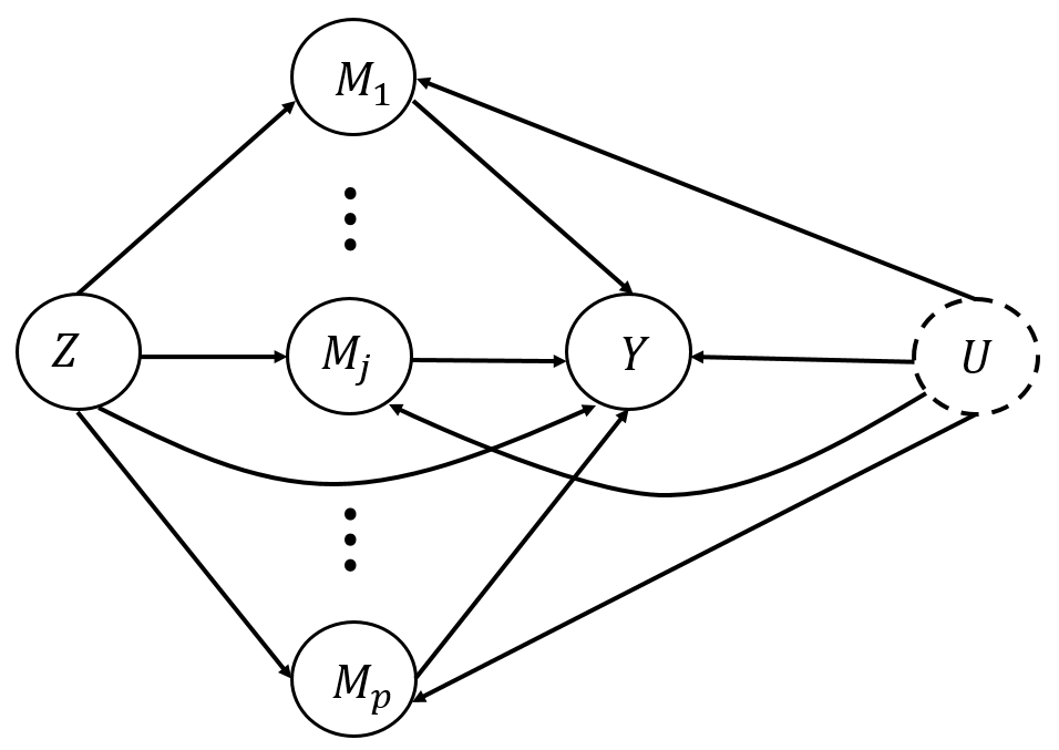
Figure 1: A causal graph with multiple causally independent mediators $M=(M_{1},\ldots,M_{p})$ and unmeasured confounders $U$.

Let $g(Z,X)=E(M\mid Z,X)\in\mathbb{R}^{p}$ and $\check{M}=M-g(Z,X)$, which represent the regression mean and residual of the mediator on treatment and observed covariates, respectively. We propose the following structural equation models involving unmeasured variables $U$:

$$Y =\beta_{0}+\beta_{1}Z+\beta_{2}^{{\mathrm{\scriptscriptstyle T}}}M+\beta_{3}^{{\mathrm{\scriptscriptstyle T}}}X+\varphi^{{\mathrm{\scriptscriptstyle T}}}U+\eta,$$ (1)

$$\check{M} =\Gamma U+\varepsilon.$$ (2)

Here, $\beta_{2}\in\mathbb{R}^{p}$, $\beta_{3}\in\mathbb{R}^{q}$, $\varphi\in\mathbb{R}^{t}$, $\Gamma\in\mathbb{R}^{p\times t}$, $E(\eta\mid Z,X)=E(\varepsilon\mid Z,X)=0$, and $U$, $\varepsilon$, and $\eta$ are mutually uncorrelated. Although the treatment $Z$ is assumed to be of one-dimension here, it is also allowed to be multi-dimensional in the models. As will be shown in the supplement, the proposed approach can be extended to include additional nonlinear or interaction terms in the outcome model. However, for the sake of clarity, we focus on the simple yet commonly-used linear model throughout the paper. Let $\beta=(\beta_{0},\beta_{1},\beta_{2}^{\mathrm{\scriptscriptstyle T}},\beta_{3}^{\mathrm{\scriptscriptstyle T}})^{\mathrm{\scriptscriptstyle T}}$ and $\xi=(\beta^{\mathrm{\scriptscriptstyle T}},\varphi^{\mathrm{\scriptscriptstyle T}})^{\mathrm{\scriptscriptstyle T}}$. Model (2) implicitly assumes $E(U\mid Z,X)=0$, which can be further relaxed by allowing $X$ to influence $U$. Specifically, if $U=\Psi X+\tilde{U}$ and $E(\tilde{U}\mid Z,X)=0$, then $\tilde{U}$ can replace $U$ in models (1) and (2). Without loss of generality, we assume $E(U)=0_{t}$, $\mathrm{cov}(U)=I_{t}$. As previously assumed, the mediators do not affect each other, and hence $\Sigma_{\varepsilon}=\mathrm{cov}(\varepsilon)$ in (2) is diagonal. This essentially implies a latent factor model in (2). Then the parameter $\Sigma_{\varepsilon}$ can be identifiable and the factor loading matrix $\Gamma$ is identifiable up to some rotation under certain conditions (Anderson et al., 1956). Under (1) and (2), we have: $\mathrm{NDE}=\beta_{1}(z-z^{\prime})$, and $\mathrm{NIE}=\beta_{2}^{\text{T}}E\{g(z,X)-g(z^{\prime},X)\}$. Similarly, the natural indirect effect through $M_{j}$ is: $\mathrm{NIE}_{j}=E[Y\{z,M_{j}(z)\}-Y\{z,M_{j}(z^{\prime})\}]=\beta_{2j}E\{g_{j}(z,X)-g_{j}(z^{\prime},X)\}$, where $g_{j}(z,X)$ represents the $j$th component of $g(z,X)$. From these equations, we conclude that estimating the direct and indirect effects hinges on estimating $\beta_{1}$ and $\beta_{2}$ in model (1).

The outcome model involves the unmeasured confounding $U$, which poses challenges in identifying and estimating model parameters. Directly applying ordinary least squares to regress $Y$ on $Z,M,X$ will yield biased estimates due to the correlation between $U$ and $M$. To address this issue, we employ projection techniques to extract the correlated component from $U$, ensuring that the projection residual and $M$ are uncorrelated. Specifically, through $L_{2}$ projection, we can select $\Delta\in\mathbb{R}^{p\times t}$ such that $\mathrm{cov}(U-\Delta^{\mathrm{\scriptscriptstyle T}}\check{M},\check{M})=0$, and by model (2), we find $\Delta=(\Gamma\Gamma^{{\mathrm{\scriptscriptstyle T}}}+\Sigma_{\varepsilon})^{-1}\Gamma\in\mathbb{R}^{p\times t}$. Defining $L=\Delta^{{\mathrm{\scriptscriptstyle T}}}\check{M}\in\mathbb{R}^{t}$ and $\psi=\varphi^{{\mathrm{\scriptscriptstyle T}}}(U-L)+\eta$, we can reformulate model (1) as:

$$Y=\beta_{0}+\beta_{1}Z+\beta_{2}^{{\mathrm{\scriptscriptstyle T}}}M+\beta_{3}^{{\mathrm{\scriptscriptstyle T}}}X+\varphi^{{\mathrm{\scriptscriptstyle T}}}L+\psi,$$ (3)

where the new error term $\psi$ is uncorrelated with $Z,M,X,L$. It is important to note that the term $\varphi^{{\mathrm{\scriptscriptstyle T}}}U$ in model (1) has been replaced by $\varphi^{{\mathrm{\scriptscriptstyle T}}}L$ in model (3), and hence $L$ can be seen as a proxy for the unmeasured confounder $U$. However, while the sequential ignorability assumption holds for the true unmeasured confounder $U$, the same assumption generally does not hold for $L$, differing from the identification strategy proposed by Yuan and Qu (2023). Based on (3), we next discuss the identification of model parameters.

Theorem 1.

The vector of parameters $\beta$ is identifiable, and $\varphi$ is identifiable up to some rotation if the following conditions hold:

• after deleting any row of $\Gamma$, there remain two disjoint sub-matrices of full column rank;

• the matrix $H=E\{(1,Z,M^{{\mathrm{\scriptscriptstyle T}}},X^{{\mathrm{\scriptscriptstyle T}}},L^{{\mathrm{\scriptscriptstyle T}}})^{{\mathrm{\scriptscriptstyle T}}}(1,Z,M^{{\mathrm{\scriptscriptstyle T}}},X^{{\mathrm{\scriptscriptstyle T}}},L^{{\mathrm{\scriptscriptstyle T}}})\}$ is of full rank.

Condition (i) in Theorem 1 is a standard requirement for identification in factor analysis. This condition ensures $\Gamma$ to be identifiable up to some rotation. When $U\in\mathbb{R}^{1}$, this condition requires $\Gamma$ to be a vector containing at least three non-zero components, implying that $U$ must confound at least three different mediators. If $U\in\mathbb{R}^{t}$, the factor loading matrix $\Gamma$ must contain at least $2t+1$ rows, which implies that there are at least $2t+1$ different mediators, and condition (i) further requires that each variable in $U$ should confound at least three different mediators. Condition (ii) involves the constructed predictor $L=\Delta^{{\mathrm{\scriptscriptstyle T}}}\check{M}$, which, given a fixed value of $\check{M}$, is identifiable up to a rotation. Although $L$ is not completely identifiable, condition (ii) can be tested for any chosen rotation. The proof in the supplement demonstrates that if condition (ii) holds for a specific rotation of $L$, it will also hold for any other rotation. Thus, without loss of generality, we can fix the rotation for ease of exposition. By the definition of $L$, it is clear that condition (ii) essentially requires the vector-valued function $g(Z,X)$ to contain some nonlinear terms of treatment and baseline covariates. Below we provide an example to illustrate our identification conditions.

Example 1.

Suppose $X,U\in\mathbb{R}^{1},M=(M_{1},M_{2},M_{3})^{{\mathrm{\scriptscriptstyle T}}}$. We consider the following models:

$$Y =Z+M_{1}+M_{2}+M_{3}+X+U+\eta,$$

$$M_{1} =Z+X+ZX+U+\varepsilon_{1},$$

$$M_{2} =Z+X+U+\varepsilon_{2},$$

$$M_{3} =Z+X+U+\varepsilon_{3},$$

where each predictor and residual are of zero mean and unit variance, and the residuals are mutually independent. In this context, $\Gamma=(1,1,1)^{{\mathrm{\scriptscriptstyle T}}}$, thus fulfilling condition $(i)$. Furthermore, we have

$$\Delta=(\Sigma_{\varepsilon}+\Gamma\Gamma^{{\mathrm{\scriptscriptstyle T}}})^{-1}\Gamma=\dfrac{\Sigma_{\varepsilon}^{-1}\Gamma}{1+\Gamma^{{\mathrm{\scriptscriptstyle T}}}\Sigma_{\varepsilon}^{-1}\Gamma}=\dfrac{\Gamma}{4}.$$

Consequently, we obtain $L=\Delta^{{\mathrm{\scriptscriptstyle T}}}\check{M}=(M_{1}+M_{2}+M_{3}-3Z-3X-ZX)/4$. Condition $(ii)$ is also met due to the inclusion of the interaction term between $Z$ and $X$ within $L$.

Example 1 illustrates that our approach only requires $M_{1}$ to include the interaction term $ZX$ for identification. In contrast, the key assumption for identification in Zheng and Zhou (2015) requires the vector $\{Z-E(Z\mid X),E(M\mid Z,X)-E(M\mid X)\}$ to be non-degenerate under our model setting. A vector of random variables $(V_{1},\cdots,V_{k})$ is considered to be non-degenerate if, for all $\lambda_{1},\cdots,\lambda_{k}\in\mathbb{R}^{1}$, the condition $E(\sum_{i=1}^{k}\lambda_{i}V_{i})^{2}=0\Leftrightarrow\lambda_{1}=\cdots=\lambda_{k}=0$ holds. In Example 1, $\{Z-E(Z\mid X),E(M\mid Z,X)-E(M\mid X)\}=\{Z-E(Z\mid X)\}(1,1+X,1,1)$ is degenerate and the identification assumption by Zheng and Zhou (2015) fails. Their assumption can be satisfied if all three mediators include distinct interaction terms between treatment and baseline covariates. Meanwhile, the heterogeneity condition of Wickramarachchi et al. (2023) requires $\mathrm{var}(M\mid Z=z,X=x)$ to vary with $z$. However, in this example, the conditional variance is a constant vector. When each $M_{j}$ incorporates a heterogeneous residual term $\varepsilon_{j}Z$ within the corresponding model, the conditional variance will vary with respect to $z$.

Our identification conditions employ interaction or nonlinear terms in certain mediator models as instruments rather than auxiliary variables. This approach aligns with common practices within the mediation analysis literature (Ten Have et al., 2007; Small, 2012; Zheng and Zhou, 2015). Example 1 shows potentials of multiple mediators for identification due to their shared-confounding structure. We further illustrate our identification strategy through the following example and highlight its difference from the null-treatment or sparsity assumptions in two related papers by Miao et al. (2023) and Tang et al. (2023) that focus on multi-treatment problems, which also exploit the shared confounding structure.

Example 2.

Consider the model presented in (1)-(2), where $M\in\mathbb{R}^{p}$, and all other variables $Z,X,U,\eta,\varepsilon_{j}$ are of one-dimension, zero mean and unit variance for $j=1,\ldots,p$. Let

$$\beta_{2}=(1,1,1,1,1,\underbrace{0,\ldots,0}_{p-5})^{\mathrm{\scriptscriptstyle T}},~{}~{}\Gamma=(1,\ldots,1,\underbrace{0,\ldots,0}_{p-10})^{\mathrm{\scriptscriptstyle T}}.$$

The null treatment strategy outlined in Miao et al. (2023) assumes that the cardinality of $\mathcal{E}\cap\mathcal{F}$ should not exceed $(\lvert\mathcal{E}\rvert-t)/2$, where $\mathcal{E}$ and $\mathcal{F}$ represent index sets of confounded treatments and active treatments that have non-zero effects on the outcome respectively in a multi-treatment scenario. Here, $t$ is the dimension of unmeasured confounding. By adapting this strategy to the context of the current mediation analysis, we find that $\lvert\mathcal{E}\cap\mathcal{F}\rvert=5$, which is greater than $(\lvert\mathcal{E}\rvert-t)/2=(10-1)/2=4.5$. This fails to meet the null treatment assumption. Since $t=1$, we deduce from Example 1 that $\Delta=(1+\Gamma^{\mathrm{\scriptscriptstyle T}}\Sigma_{\varepsilon}^{-1}\Gamma)^{-1}\Sigma_{\varepsilon}^{-1}\Gamma$. The identification assumption of the synthetic instrument approach by Tang et al. (2023) necessitates the invertibility of any $t\times t$ submatrix of $\Delta$. Here the invertibility of $\Delta$ requires that all components in $\Gamma$ are nonzero, which does not hold true in our context. In contrast, our identification assumption can be satisfied when $g_{j}(Z,X)$ is a nonlinear function of $Z$ and $X$ for some $j=1,\cdots,10$, as shown in the simulation studies.

3 Estimation and Inference

In this section, we present a partially penalized procedure for estimating outcome model parameters when $\beta_{2}$ is assumed to be sparse. Due to the curse of dimensionality, conducting nonparametric estimation of $g(Z,X)$ often becomes impractical, especially when dealing with a large number of covariates. We thus propose a semiparametric model $g(Z,X;\gamma)$ parameterized by a finite-dimensional vector $\gamma\in\mathbb{R}^{k}$. Let the operator $\hat{E}[\cdot]$ denote the sample averaging operation. For a matrix $V$, let $\mathrm{vec}(V)$ denote the vectorization of $V$ and $\mathrm{diag}(V)$ the vector consisting of the diagonal elements of $V$.

Denote $\check{M}(\gamma)=M-g(Z,X;\gamma)$ and $\nu=\mathrm{vec}[\{\gamma,\Gamma,\mathrm{diag}(\Sigma_{\varepsilon})\}]$. Let $\hat{\gamma},\hat{\Gamma},\hat{\Sigma}_{\varepsilon},\hat{\nu}$ be the estimates of $\gamma,\Gamma,\Sigma_{\varepsilon},\nu$, respectively. The estimation procedure is summarized as follows:

• Solve the minimization problem $\mathop{\min}_{\gamma}\hat{E}\lVert\check{M}(\gamma)\rVert_{2}^{2}$ to obtain $\hat{\gamma}$ and denote $\check{M}(\hat{\gamma})=M-g(Z,X;\hat{\gamma})$, where $\lVert\cdot\rVert_{2}$ represents the $\ell_{2}$ norm;

• Implement factor analysis on $\check{M}(\hat{\gamma})$ to obtain $\hat{\Gamma}$ and $\hat{\Sigma}_{\varepsilon}$, then obtain $\hat{\Delta}=(\hat{\Gamma}\hat{\Gamma}^{\mathrm{\scriptscriptstyle T}}+\hat{\Sigma}_{\varepsilon})^{-1}\hat{\Gamma}$ and an estimate $\hat{L}=\hat{\Delta}^{\mathrm{\scriptscriptstyle T}}\check{M}(\hat{\gamma})$ of the proxy variable $L$;

• Solve the following adaptive lasso problem to obtain $\hat{\beta}_{\mathrm{ad}}$:

  $$\hat{\beta}_{\mathrm{ad}}=\mathop{\arg\min}_{\beta,\varphi}\hat{E}\big{(}Y-\beta_{0}-\beta_{1}Z-\beta_{2}^{\mathrm{\scriptscriptstyle T}}M-\beta_{3}^{\mathrm{\scriptscriptstyle T}}X-\varphi^{\mathrm{\scriptscriptstyle T}}\hat{L}\big{)}^{2}+\dfrac{\lambda_{n}}{n}\sum_{r=1}^{p}\hat{w}_{r}\lvert\beta_{2,r}\rvert,$$ (4)

  where $\hat{w}=\lvert\hat{\beta}_{\mathrm{in},2}\rvert^{-\delta}$ using an initial $\sqrt{n}$-consistent estimator $\hat{\beta}_{\mathrm{in},2}$ of $\beta_{2}$, and $\delta,\lambda_{n}>0$ are tuning parameters.

Step (1) corresponds to solving $k$ estimating equations to obtain $\hat{\gamma}$. Since $E\{\check{M}(\gamma)\mid Z,X\}=0$, it follows that $E\{\check{M}(\gamma)G(Z,X)\}=0$ for any function $G(\cdot)$. Particularly, the minimization problem $\mathop{\min}_{\gamma}\hat{E}\lVert\check{M}(\gamma)\rVert_{2}^{2}$ in step (1) corresponds to solving the following estimating equations:

$$\hat{E}\bigg{\{}\check{M}(\gamma)^{\mathrm{\scriptscriptstyle T}}\dfrac{\partial g(Z,X;\gamma)}{\partial\gamma^{\mathrm{\scriptscriptstyle T}}}\bigg{\}}=0.$$ (5)

The estimation procedure for $\Gamma$ and $\Sigma_{\varepsilon}$ in step (2) is performed by maximizing the following normal likelihood function, assuming $U\sim N(0,I_{t})$ and $\varepsilon\sim N(0,\Sigma_{\varepsilon})$ (Anderson et al., 1956): $l(\Gamma,\Sigma_{\varepsilon})=-\log\lvert\Sigma\rvert-\mathrm{tr}(T_{n}\Sigma^{-1})$, where $T_{n}=\hat{E}\{\check{M}(\gamma)\check{M}(\gamma)^{\mathrm{\scriptscriptstyle T}}\},\Sigma=\Gamma\Gamma^{\mathrm{\scriptscriptstyle T}}+\Sigma_{\varepsilon}$ and $\mathrm{tr}(\cdot)$ represents the trace operator. It is worth noting that the normal assumption is not essential in factor analysis because we can treat the likelihood as a quasi-likelihood. Maximizing the above likelihood function in step (2) is equivalent to solving (5) and the following estimating equations:

$$\hat{E}\bigg{[}\dfrac{\partial}{\partial\alpha}\big{\{}\log\lvert\Sigma\rvert+\check{M}(\gamma)^{\mathrm{\scriptscriptstyle T}}\Sigma^{-1}\check{M}(\gamma)\big{\}}\bigg{]}=0,$$ (6)

where $\alpha=\mathrm{vec}[\{\Gamma,\mathrm{diag}(\Sigma_{\varepsilon})\}]$. Different from the classical adaptive lasso problem (Zou, 2006), the minimization problem in (4) involves an estimated variable $\hat{L}$ for $L$ and partially penalizes $\beta_{2}$ rather than the entire parameter vector. This introduces complexity in the theoretical analysis, because it requires consideration of additional uncertainty when deriving the asymptotic results of the proposed estimator.

Theorem 1 shows that $\beta$ is identifiable, although the factor loading $\Gamma$ is identifiable only up to a rotation matrix. To ensure identifiability of $\Gamma$, a second condition is commonly imposed (Anderson et al., 1956; Bai and Li, 2012); that is, $\Gamma^{\mathrm{\scriptscriptstyle T}}\Sigma_{\varepsilon}^{-1}\Gamma$ is assumed to be diagonal, with distinct positive elements arranged in decreasing order. For the convenience of theoretical analysis, we retain this second condition to fix the rotation matrix of $\Gamma$. The asymptotic distribution of the estimator of $\beta_{2}$ remains unaffected by the rotation matrix. In other words, we can replace $\Gamma$ with $\Gamma A$ for any orthogonal matrix $A$, and the conclusions presented in this section will remain valid. We define

$$Q(S;\nu)=\bigg{[}\check{M}(\gamma)^{\mathrm{\scriptscriptstyle T}}\dfrac{\partial g(Z,X;\gamma)}{\partial\gamma^{\mathrm{\scriptscriptstyle T}}},\dfrac{\partial}{\partial\alpha^{\mathrm{\scriptscriptstyle T}}}\big{\{}\check{M}(\gamma)^{\mathrm{\scriptscriptstyle T}}{\Sigma}^{-1}\check{M}(\gamma)+\log\lvert\Sigma\rvert\big{\}}\bigg{]}^{\mathrm{\scriptscriptstyle T}},$$

where $S=(Z,M^{\mathrm{\scriptscriptstyle T}},X^{\mathrm{\scriptscriptstyle T}})^{\mathrm{\scriptscriptstyle T}}$. Then we can summarize the estimating equations in (5) and (6) as follows: $\hat{E}\{Q(S;\nu)\}=0$. The estimator $\hat{\nu}$ is derived by solving these equations. Under certain regularity conditions, $\hat{\nu}$ is $\sqrt{n}$-consistent for $\nu_{0}$ and asymptotically normal, where $\nu_{0}$ denotes the true value of $\nu$.

The initial $\sqrt{n}$-consistent estimator $\hat{\beta}_{\mathrm{in},2}$ in step (3) can be computed using various methods, such as ordinary least squares or the lasso procedure. However, when dealing with potentially many predictors, the lasso-type estimator is often preferred, especially when the true parameter is assumed to have a sparse structure. In this context, we present an initial lasso estimator, denoted as $\hat{\xi}_{\mathrm{la}}$, for $\xi$. This estimator is derived by partially penalizing $\beta_{2}$ in the following problem:

$$\hat{\xi}_{\mathrm{la}}=(\hat{\beta}_{\mathrm{la}}^{\mathrm{\scriptscriptstyle T}},\hat{\varphi}_{\mathrm{la}}^{\mathrm{\scriptscriptstyle T}})^{\mathrm{\scriptscriptstyle T}}=\mathop{\arg\min}_{\beta,\varphi}\hat{E}\big{(}Y-\beta_{0}-\beta_{1}Z-\beta_{2}^{\mathrm{\scriptscriptstyle T}}M-\beta_{3}^{\mathrm{\scriptscriptstyle T}}X-\varphi^{\mathrm{\scriptscriptstyle T}}\hat{L}\big{)}^{2}+\dfrac{\lambda_{n}}{n}\sum_{r=1}^{p}\lvert\beta_{2,r}\rvert.$$

Let $R=(1,Z,M^{\mathrm{\scriptscriptstyle T}},X^{\mathrm{\scriptscriptstyle T}},L^{\mathrm{\scriptscriptstyle T}})^{\mathrm{\scriptscriptstyle T}}$, and $R_{i}$ represents the $i$th realization of $R$. We summarize the $\sqrt{n}$-consistency of $\hat{\xi}_{\mathrm{la}}$ in the following theorem.

Theorem 2.

Suppose that $\lambda_{n}=o_{p}(\sqrt{n})$ and the following conditions are satisfied:

• $n^{-1}\max_{1\leq i\leq n}R_{i}R_{i}^{\mathrm{\scriptscriptstyle T}}\to 0$, and ${C}_{n}=n^{-1}\sum_{i=1}^{n}R_{i}R_{i}^{\mathrm{\scriptscriptstyle T}}\to C$ for a positive definite matrix $C$;

• For $1\leq i,j\leq t$, the following expectations exist:

  $$E\bigg{\{}R\dfrac{\partial L_{j}(\nu_{0})}{\partial\nu^{\mathrm{\scriptscriptstyle T}}}\bigg{\}},\quad\text{and}\quad E\bigg{\{}\dfrac{\partial L_{i}(\nu_{0})}{\partial\nu}\dfrac{\partial L_{j}(\nu_{0})}{\partial\nu^{\mathrm{\scriptscriptstyle T}}}\bigg{\}};$$

• $E(KK^{\mathrm{\scriptscriptstyle T}})$ exists, where

  $$K=E\bigg{[}R\dfrac{\partial\{\varphi^{\mathrm{\scriptscriptstyle T}}L(\nu_{0})\}}{\partial\nu^{\mathrm{\scriptscriptstyle T}}}\bigg{]}\bigg{[}\dfrac{\partial E\{Q(S;\nu_{0})\}}{\partial\nu}\bigg{]}^{-1}Q(S;\nu_{0})+R\psi.$$

Then under additional regularity conditions provided in the supplement, we have:

$$\sqrt{n}\big{(}\hat{\xi}_{\mathrm{la}}-\xi\big{)}\overset{d}{\longrightarrow}N(0,\Sigma_{\mathrm{la}}),$$

where $\Sigma_{\mathrm{la}}=C^{-1}E\big{(}KK^{\mathrm{\scriptscriptstyle T}}\big{)}C^{-1}$.

The uncertainty associated with $\hat{\xi}_{\mathrm{la}}$ in Theorem 2 stems from two distinct sources. Firstly, it comes from the procedure employed to estimate the parameters of $\nu_{0}$, and secondly, it arises from the process of estimating $\beta$ through the partially penalized least squares method. If the true value $\nu_{0}$ or $L$ were known, the optimization problem would become a standard lasso problem with a partial penalization term. Consequently, the covariance matrix $\Sigma_{\mathrm{la}}$ would be simplified to $C^{-1}E\big{(}R\psi^{2}R^{\mathrm{\scriptscriptstyle T}}\big{)}C^{-1}$. This demonstrates that the first term within $K$ accounts for the uncertainty in estimation of the constructed proxy variable $L$, which is also the impact of unmeasured confounding $U$ on the estimation of $\beta$.

As shown in Theorem 1, $\beta$ is identifiable while $\varphi$ is only identifiable up to some rotation, which implies that the constructed predictor $L$, and therefore $R$, are not completely identifiable. This raises an important question of whether the asymptotic normality of $\hat{\beta}_{\mathrm{la}}$ in Theorem 2 depends on the rotation of $R$. In particular, suppose that $R$ is replaced by $PR$ with $P$ defined as follows:

$$P=\begin{pmatrix}I_{p+q+2}&0\\ 0&A\end{pmatrix},$$

and $A$ denotes a rotation matrix that satisfies $AA^{\mathrm{\scriptscriptstyle T}}=A^{\mathrm{\scriptscriptstyle T}}A=I_{t}$. In this situation, because $\varphi^{\mathrm{\scriptscriptstyle T}}L$ is identifiable, the variable $K$ in condition (iii) of Theorem 2 will similarly be replaced by $PK$, leading to an asymptotic variance of $\sqrt{n}\big{(}\hat{\xi}_{\mathrm{la}}-\xi\big{)}$ represented by:

$$\big{(}PCP^{\mathrm{\scriptscriptstyle T}}\big{)}^{-1}\big{\{}PE(KK^{\mathrm{\scriptscriptstyle T}})P^{\mathrm{\scriptscriptstyle T}}\big{\}}\big{(}PCP^{\mathrm{\scriptscriptstyle T}}\big{)}^{-1}=P\Sigma_{\mathrm{la}}P^{\mathrm{\scriptscriptstyle T}}=\begin{pmatrix}\Sigma_{11}&\Sigma_{12}A^{\mathrm{\scriptscriptstyle T}}\\ A\Sigma_{12}^{\mathrm{\scriptscriptstyle T}}&A\Sigma_{22}A^{\mathrm{\scriptscriptstyle T}}\end{pmatrix},$$

where $\Sigma_{ij}$’s $(i,j=1,2)$ are block matrices of $\Sigma_{\mathrm{la}}$. It is thus evident that the asymptotic variance of $\hat{\varphi}_{\mathrm{la}}$ and its asymptotic covariance with estimators of $\beta$ may be influenced by the rotation of $R$. However, the asymptotic variance of $\hat{\beta}_{\mathrm{la}}$ remains unaffected by any rotation of $R$.

Building upon the $\sqrt{n}$-consistent lasso estimator, we proceed to construct an initial estimator with all non-zero elements for $\beta_{2}$, given by $\hat{\beta}_{\mathrm{in},2}=\hat{\beta}_{\mathrm{la},2}+n^{-1}$, and introduce the adaptive weight $\hat{w}=\lvert\hat{\beta}_{\mathrm{in},2}\rvert^{-\delta}$ for some $\delta>0$. Let $\mathcal{A}$ be the set of indices corresponding to the non-zero elements of $\beta_{2}$, and $\hat{\mathcal{A}}_{n}$ represent the set of indices for non-zero elements of $\hat{\beta}_{\mathrm{ad},2}$; that is, $\mathcal{A}=\{j:\beta_{2j}\neq 0\}$ and $\hat{\mathcal{A}}_{n}=\{j:\hat{\beta}_{\mathrm{ad},2j}\neq 0\}$. We then define $\tilde{\mathcal{A}}$ as the union of index sets of $\beta_{0}$, $\beta_{1}$, $\beta_{2,\mathcal{A}}$, $\beta_{3}$, and $\varphi$.

Theorem 3.

Suppose conditions in Theorem 2 hold and $\lambda_{n}n^{(\delta-1)/2}\to\infty$. Then we have

• consistency in variable selection: $\lim_{n\to\infty}P(\hat{\mathcal{A}}_{n}=\mathcal{A})=1$,

• asymptotic normality: $\sqrt{n}(\hat{\xi}_{\mathrm{ad},\tilde{\mathcal{A}}}-\xi_{\tilde{\mathcal{A}}})\overset{d}{\longrightarrow}N(0,\Sigma_{\mathrm{ad}})$,

where $\hat{\xi}_{\mathrm{ad}}=(\hat{\beta}_{\mathrm{ad}}^{\mathrm{\scriptscriptstyle T}},\hat{\varphi}_{\mathrm{ad}}^{\mathrm{\scriptscriptstyle T}})^{\mathrm{\scriptscriptstyle T}},\Sigma_{\mathrm{ad}}=\tilde{C}^{-1}E(K_{\tilde{\mathcal{A}}}K_{\tilde{\mathcal{A}}}^{\mathrm{\scriptscriptstyle T}})\tilde{C}^{-1}$, and $\tilde{C}=C_{\tilde{\mathcal{A}},\tilde{\mathcal{A}}}.$

Theorem 3 shows that the adaptive lasso estimator $\hat{\beta}_{\mathrm{ad}}$ enjoys the oracle property. Specifically, the estimator $\hat{\beta}_{\mathrm{ad}}$ successfully identifies the true nonzero elements of $\beta_{2}$ with probability asymptotically approaching 1, and the joint asymptotic distribution of the estimator $\hat{\beta}_{\mathrm{ad}}$ and $\hat{\varphi}_{\mathrm{ad}}$ is the same as if the true underlying subset model were given in advance. The optimal values of the tuning parameters are chosen through cross-validation procedures. We have previously demonstrated that the asymptotic variance of $\hat{\beta}_{\mathrm{la}}$ remains unaffected by the rotation of $R$. The same holds true for the adaptive lasso estimator $\hat{\beta}_{\mathrm{ad}}$, with $C$ and $K$ replaced by $\tilde{C}$ and $K_{\tilde{\mathcal{A}}}$ in its asymptotic variance. The asymptotic variance $\Sigma_{\mathrm{ad}}$ can be estimated using the observed data. Specifically, we can directly estimate $C$ by employing the sample mean $C_{n}=\hat{E}(RR^{\mathrm{\scriptscriptstyle T}})$. Likewise, $E(KK^{\mathrm{\scriptscriptstyle T}})$ can also be estimated using the sample mean, incorporating estimators of all relevant parameters. By incorporating these estimators along with the estimated index set $\hat{\mathcal{A}}_{n}$, we can construct a consistent estimate of the asymptotic variance for the adaptive lasso estimator.

Because $\mathrm{NDE}=\beta_{1}(z-z^{\prime})$, the asymptotic normality of the estimator $\hat{\beta}_{\mathrm{ad},1}$ in Theorem 3 allows us to evaluate the significance of the natural direct effect. The indirect effect through the $j$th mediator, denoted as $\mathrm{NIE}_{j}$, is equal to $\beta_{2j}\lambda_{j}$, with $\lambda_{j}=E\{g_{j}(z,X;\gamma)-g_{j}(z^{\prime},X;\gamma)\}$. Traditional approaches for selecting active mediation pathways often involve performing the composite null hypothesis for each mediator: $\beta_{2j}\lambda_{j}=0$, which is complicated in practice (Huang, 2019; Liu et al., 2022). Leveraging the selection consistency of the adaptive lasso estimator $\hat{\beta}_{\mathrm{ad},2}$, we can simplify the process of identifying active mediation pathways. Specifically, Theorem 3 implies that, the mediators truly affecting the outcome can be asymptotically selected due to the oracle property of $\hat{\beta}_{\mathrm{ad},2}$. To determine the active mediation pathways, one can subsequently test whether $\lambda_{j}=0$ among the selected mediators to identify those also influenced by the treatment variable. For example, when $g(Z,X)=\gamma_{1}Z+\gamma_{2}X+\gamma_{3}X^{2}$, the term $\lambda_{j}=\gamma_{1j}(z-z^{\prime})$, and it suffices to test whether $\gamma_{1j}=0$ for $j\in\hat{\mathcal{A}}_{n}$ using the standard $t$-test method. More generally, one can construct an estimator $\hat{\lambda}_{j}=\hat{E}\{g_{j}(z,X;\hat{\gamma})-g_{j}(z^{\prime},X;\hat{\gamma})\}$ for $\lambda_{j}$, and subsequently calculate the corresponding $z$-score to test whether $\lambda_{j}=0$ for $j\in\hat{\mathcal{A}}_{n}$. We summarize the two-step procedure for selecting active causal mediation pathways as follows: (1) obtain the index set $\hat{\mathcal{A}}_{n}$ from the nonzero elements of $\hat{\beta}_{\mathrm{ad},2}$; (2) for each $j\in\hat{\mathcal{A}}_{n}$, perform a hypothesis test $H_{j}:\lambda_{j}=0$. Define the index subset $\hat{\mathcal{A}}_{\mathrm{act},n}$ as the union of indices $j\in\hat{\mathcal{A}}_{n}$ for which $H_{j}$ is rejected at the significance level $\alpha_{j}$. The set $\hat{\mathcal{A}}_{\mathrm{act},n}$ represents the estimated active mediator set.

As shown above, the proposed two-step procedure for selecting active mediation pathways involves performing simple hypothesis tests $H_{j}$ for $j\in\hat{\mathcal{A}}_{n}$, without the necessity of conducting a composite null hypothesis test for all mediators. We present the following corollary to highlight that the proposed procedure can consistently select the active mediation pathways with a large probability.

Corollary 1.

Denote $\mathcal{A}_{\mathrm{act}}\subseteq\mathcal{A}$ as the true active mediator set, then under certain regularity conditions in the supplement, we have

$$\lim_{n\to\infty}P(\hat{\mathcal{A}}_{\mathrm{act},n}=\mathcal{A}_{\mathrm{act}})\geq 1-\sum_{j\in\mathcal{A}\backslash\mathcal{A}_{\mathrm{act}}}\alpha_{j}.$$

In Corollary 1, the consistency of selecting active mediation pathways hinges on controlling the probability of rejecting at least one true $H_{j}$, also known as the family-wise error rate. This error rate should not exceed the aggregate significance levels, denoted by $\sum_{j\in\mathcal{A}\backslash\mathcal{A}_{\mathrm{act}}}\alpha_{j}$. The classical Bonferroni correction method achieves error control at a predetermined significance level $\alpha$ by setting $\alpha_{j}=\alpha/h$ for each individual test $H_{j}$, where $h=|\hat{\mathcal{A}}_{n}|$ denotes the number of selected mediators in the first step. However, given the potential conservatism of the Bonferroni correction when $h$ is large, one can also adopt more powerful multiple testing techniques, such as Holm’s method, Hochberg’s method or the Benjamini-Hochberg procedure (Benjamini and Hochberg, 1995), as implemented in our application section.

4 Simulation

In this section, we conduct simulation studies to assess the finite-sample performance of the proposed estimator. We compare our approach with two naive penalized regression methods, the naive lasso and naive adaptive lasso, which do not account for unmeasured mediator-outcome confounding. We generate the outcome $Y$ and mediators $M\in\mathbb{R}^{p}$ based on the following models:

$$Y =\beta_{1}Z+\beta_{2}^{\mathrm{\scriptscriptstyle T}}M+\beta_{3}X+\varphi U+\eta,$$

$$M =\gamma_{1}Z+\gamma_{2}X+\gamma_{3}\exp(X)+\Gamma U+\varepsilon.$$

Table 1: Simulation results of the mean squared error (MSE), the number of true positives (TP) and the number of false negatives (FP) for estimating $\beta_{2}$ by the proposed approach, naive lasso and naive adaptive lasso in scenario 1.

		Proposed approach				Naive lasso				Naive adaptive lasso
$p$		100	200	300		100	200	300		100	200	300
	MSE	0.06	0.03	0.03		0.12	0.12	0.11		0.15	0.15	0.15
$n=300,\varphi=1$	TP	5	5	5		5	5	5		5	5	5
	FP	0.07	0	0		11.79	14.14	15.43		0.01	0	0
	MSE	0.23	0.22	0.08		1.40	1.39	1.37		1.48	1.51	2.03
$n=300,\varphi=4$	TP	4.99	5	5		5	5	5		5	5	5
	FP	3.27	4.60	0.27		11.29	13.86	13.69		5.37	5.58	1.42
	MSE	0.02	0.02	0.02		0.10	0.10	0.10		0.14	0.14	0.14
$n=600,\varphi=1$	TP	5	5	5		5	5	5		5	5	5
	FP	0	0	0		12.54	12.75	14.72		0	0	0
	MSE	0.05	0.04	0.04		1.38	1.36	1.36		1.41	1.42	1.42
$n=600,\varphi=4$	TP	5	5	5		5	5	5		5	5	5
	FP	0.18	0.01	0		12.13	12.59	14.33		5	4.99	5
	MSE	0.01	0.01	0.01		0.09	0.09	0.09		0.13	0.13	0.13
$n=1000,\varphi=1$	TP	5	5	5		5	5	5		5	5	5
	FP	0	0	0		12.18	13.86	15.26		0	0	0
	MSE	0.04	0.03	0.03		1.37	1.37	1.35		1.39	1.39	1.39
$n=1000,\varphi=4$	TP	5	5	5		5	5	5		5	5	5
	FP	0.01	0.01	0		11.74	12.65	14.51		5	5	5

Here, $(Z,X,U,\varepsilon,\eta)$ are drawn from a multivariate normal distribution with zero mean and identity covariance matrix. We set $\beta_{1}=\beta_{3}=1$, $\gamma_{1}=\gamma_{2}=(1,1,1,1,\ldots,1)^{\mathrm{\scriptscriptstyle T}}$ and let

$$\gamma_{3} =(0.5,0.5,0.5,\underbrace{0,\ldots,0}_{p-3})^{\mathrm{\scriptscriptstyle T}},\quad\Gamma=(1,\ldots,1,\underbrace{0,\ldots,0}_{p-10})^{\mathrm{\scriptscriptstyle T}},$$

where the first three elements of $\gamma_{3}$ is non-zero, meaning that the first three mediators contain the nonlinear term $\exp(X)$, and the first ten elements of $\Gamma$ is non-zero, meaning that the unmeasured variable $U$ confounds the first ten mediators. We consider two scenarios for $\beta_{2}$:

$$\text{Scenario 1: }\beta_{2}=(1,1,1,1,1,\underbrace{0,\ldots,0}_{p-5})^{\mathrm{\scriptscriptstyle T}};~{}~{}~{}~{}\text{Scenario 2: }\beta_{2}=(1,1,1,1,1,0,\ldots,0,\underbrace{1,\ldots,1}_{15})^{\mathrm{\scriptscriptstyle T}}.$$

Scenario 1 is constructed to include five mediators that are both active and confounded, while scenario 2 incorporates additional 15 active but unconfounded mediators. We vary the sample size $n$ across $\{300,600,1000\}$ and the dimension $p$ across $\{100,200,300\}$.

Table 2: Simulation results for scenario 2. The caption details remain the same as those in Table 1.

		Proposed approach				Naive lasso				Naive adaptive lasso
$p$		100	200	300		100	200	300		100	200	300
	MSE	0.38	0.18	0.26		0.36	0.46	0.52		0.30	0.31	0.52
$n=300,\varphi=1$	TP	19.93	20	20		20	20	20		20	20	20
	FP	0.29	0.05	0.04		33.12	49.34	54.21		0.01	0	0
	MSE	0.63	0.41	0.45		1.99	2.18	2.30		1.68	1.73	4.49
$n=300,\varphi=4$	TP	19.93	19.99	19.99		20	20	20		20	20	19.81
	FP	1.89	2.72	0.15		31.48	46.65	55.24		5.27	6.66	1.52
	MSE	0.12	0.11	0.11		0.24	0.25	0.28		0.24	0.25	0.24
$n=600,\varphi=1$	TP	20	20	20		20	20	20		20	20	20
	FP	0.01	0.01	0		22.35	44.81	57.34		0	0	0
	MSE	0.24	0.21	0.19		1.67	1.74	1.80		1.49	1.51	1.51
$n=600,\varphi=4$	TP	20	20	20		20	20	20		20	20	20
	FP	0.17	0.30	0		32.69	44.95	53.46		5.00	4.94	4.98
	MSE	0.09	0.09	0.09		0.21	0.21	0.21		0.22	0.22	0.22
$n=1000,\varphi=1$	TP	20	20	20		20	20	20		20	20	20
	FP	0	0	0		10.31	23.88	44.38		0	0	0
	MSE	0.16	0.13	0.14		1.55	1.59	1.61		1.44	1.44	1.44
$n=1000,\varphi=4$	TP	20	20	20		20	20	20		20	20	20
	FP	0.10	0.02	0		32.69	45.68	53.96		5	5	5

Given that the effect of $Z$ on each $M_{j}$ has been fixed at 1, an individual mediation pathway is active whenever the effect of $M_{j}$ on $Y$ is non-zero. Thus, our focus lies in assessing precision of estimating $\beta_{2}$ and the selection consistency. We compute the mean squared error (MSE) of each estimator, which is the sum of mean squared errors across the coordinates of the estimator: $\mathrm{MSE}=\sum_{j=1}^{p}(\hat{\beta}_{2j}-\beta_{2j})^{2}$, where $\hat{\beta}_{2j}$ denotes an estimator of $\beta_{2j}$ for $j=1,\ldots,p$. We also calculate the number of true positives (TP) and false positives (FP) in estimating $\beta_{2}$. The results of MSE, TP, and FP for all methods, averaged over 200 experiments, are presented in Tables 1 and 2 for scenarios 1 and 2, respectively.

The results in Table 1 indicate a significantly smaller MSE for our approach compared to the naive lasso and naive adaptive lasso methods. Notably, as the unmeasured confounding strength $\varphi$ increases from 1 to 4, the advantage of our approach becomes more apparent in terms of MSE, particularly evident in larger sample sizes. From the TP results, we find that all methods appear to correctly identify the mediators that genuinely affect the outcome across various scenarios. However, concerning FP, our approach exhibits superior performance compared to the other two. The naive lasso exhibits the highest FP among the three methods. For cases with weaker unmeasured confounding strength (i.e., $\varphi=1$), the naive adaptive lasso demonstrates similar performance to our approach, both yielding nearly zero FP. However, as $\varphi$ increases, the FP of our approach remains consistently lower than that of the naive adaptive lasso in all scenarios. Moreover, with larger sample sizes, the FP of our approach converges to approximately zero, whereas the naive adaptive lasso maintains an FP of around 5. This value aligns with the number of mediators confounded by $U$ yet not affecting the outcome. This distinction highlights that our approach can effectively filter out false signals arising from unmeasured confounding, while the other two methods might incorrectly identify them as genuine signals. Similar simulation results are displayed in Table 2.

Table 3: Simulation results for scenario 1 under model (8). The parameter $\varphi_{1}$ indicates the extent of model misspecification, and the rest of the caption details remain the same as those in Table 1.

		Proposed approach				Naive lasso				Naive adaptive lasso
$p$		100	200	300		100	200	300		100	200	300
	MSE	0.03	0.03	0.03		1.37	1.36	1.37		1.40	1.39	1.39
$\varphi_{1}=0.5$	TP	5	5	5		5	5	5		5	5	5
	FP	0	0.01	0		11.54	13.84	14.95		5	5	5
	MSE	0.04	0.04	0.04		1.38	1.37	1.37		1.40	1.39	1.39
$\varphi_{1}=1$	TP	5	5	5		5	5	5		5	5	5
	FP	0	0.02	0		11.35	14.79	14.58		5	5	5
	MSE	0.06	0.07	0.07		1.39	1.39	1.38		1.40	1.39	1.39
$\varphi_{1}=1.5$	TP	5	5	5		5	5	5		5	5	5
	FP	0.02	0.41	0.69		11.39	14.85	14.35		5	5	5
	MSE	0.12	0.27	0.25		1.41	1.41	1.39		1.40	1.39	1.39
$\varphi_{1}=2$	TP	5	5	5		5	5	5		5	5	5
	FP	1.32	5.50	4.49		11.06	14.40	14.27		5	5	5

Table 4: Simulation results for scenario 2 under model (8). The parameter $\varphi_{1}$ indicates the extent of model misspecification, and the rest of the caption details remain the same as those in Table 1.

		Proposed approach				Naive lasso				Naive adaptive lasso
$p$		100	200	300		100	200	300		100	200	300
	MSE	0.15	0.19	0.15		1.58	1.62	1.66		1.44	1.44	1.44
$\varphi_{1}=0.5$	TP	20	20	20		20	20	20		20	20	20
	FP	0.01	0.03	0		31.90	46.08	55.38		5	5	5
	MSE	0.19	0.22	0.18		1.65	1.73	1.77		1.44	1.44	1.44
$\varphi_{1}=1$	TP	20	20	20		20	20	20		20	20	20
	FP	0.02	0.03	0		31.37	45.43	54.07		5	5.00	5
	MSE	0.24	0.28	0.25		1.78	1.90	1.96		1.44	1.44	1.44
$\varphi_{1}=1.5$	TP	20	20	20		20	20	20		20	20	20
	FP	0.06	0.06	0.23		30.64	44.37	53.01		5	5.00	5
	MSE	0.33	0.41	0.42		1.96	2.13	2.23		1.44	1.44	1.44
$\varphi_{1}=2$	TP	20	20	20		20	20	20		20	20	20
	FP	0.21	1.88	2.74		30.29	44.02	53.09		5	5.00	5

These simulation results demonstrate that our approach can successfully identify the mediators with significant effects on the outcome. It can also eliminate nearly all false signals when unmeasured mediator-outcome confounding is present. In contrast, the two naive methods often misinterpret mediators confounded by $U$ as valid signals. Specifically, for the more competitive naive adaptive lasso method in scenario 1, all the ten mediators confounded by $U$ are incorrectly identified as the true mediators, although half of them do not affect the outcome. Our approach can accurately differentiate between genuine signals and those that have spurious correlations with the outcome due to confounding bias. Despite the strong performance of all methods in terms of TP in the current settings, the presence of confounding bias may also lead the naive approachs to miss certain valid signals, which will induce lower TP values in certain cases for the two naive approachs.

To assess the robustness of our proposed estimator against model misspecification, we extend the analysis to generate the outcome $Y$ in the following new way:

$$Y=\beta_{1}Z+\beta_{2}^{\mathrm{\scriptscriptstyle T}}M+\beta_{3}X+\varphi U+\varphi_{1}U^{2}+\eta.$$ (8)

Here, $\beta_{1}$, $\beta_{2}$, and $\beta_{3}$ take the same values as those specified in the correctly specified model setting. We consider a relatively large sample size $n=1000$ and relatively strong unmeasured confounding with $\varphi=4$. The parameter $\varphi_{1}$ varies across $\{0.5,1,1.5,2\}$, and the results are presented in Tables 3 and 4 for the two distinct scenarios of $\beta_{2}$. Table 3 shows that our approach consistently outperforms the two naive approachs in terms of MSE, regardless of the specific value of $\varphi_{1}$. When the outcome model exhibits mild misspecification, with lower $\varphi_{1}$ values indicating less deviation, our approach can precisely exclude false signals and exhibit minimal false positives. However, in the presence of substantial misspecification, characterized by $\varphi_{1}=2$, all three methods are unable to completely avoid inducing false signals. Similar results are presented in Table 4. Overall, these findings imply that our proposed estimator can still provide good performance when the outcome model is moderately misspecified.

5 Data Analysis

In this section, we use the mouse obesity data described by Wang et al. (2006) to illustrate the proposed approach. This study focuses on evaluating the effect of gene expressions on the body weight of F2 mice. In this context, it is important to consider potential unmeasured phenotypes that might confound the gene expressions and body weight. Lin et al. (2015) employed single nucleotide polymorphisms (SNPs) as instrumental variables and introduced a high-dimensional instrumental variable regression approach for analyzing this mouse obesity dataset. However, the presence of potential pleiotropic effects poses a challenge, because the SNPs might violate the exclusion restriction assumption fundamental to instrumental variables. Among the pool of SNPs, a specific variable named rs4231406 was previously identified as a quantitative trait locus for atherosclerosis, with a significant association with both body weight and adiposity (Wang et al., 2006). Here, our goal is to investigate the direct effect of this SNP on body weight as well as its potential indirect effect through gene expressions using mediation analysis. The dataset we use includes 287 mice and comprises two observed covariates: sex and SNP density. Our analysis further incorporates the top 200 gene expressions that exhibit the strongest correlations with body weight as candidate mediators.

Table 5: Estimate and standard deviation (SD) of natural indirect effects through selected genes, and the corresponding $p$-value of testing each mediation pathway by the proposed approach. The genes framed in red are found to be active by all multiple testing correction procedures.

Gene	Estimate	SD	$p$-value		Gene	Estimate	SD	$p$-value
$$Slc39a11$$	0.131	0.072	$<10^{-3}$		Vkorc1l1	-0.038	0.124	0.205
$$Ercc3$$	0.144	0.272	0.001		Lamc1	0.0144	0.041	0.252
Psmd12	0.124	0.118	0.003		Serpina12	-0.013	0.027	0.316
Zfp533	0.172	0.275	0.005		Tbx 22	0.006	0.118	0.357
Serpina6	-0.157	0.094	0.006		Cmas	-0.019	0.129	0.522
RGD1563955	-0.139	0.121	0.012		Rn.20259	0.035	0.100	0.536
Nek2	-0.143	0.297	0.012		Psmd8	-0.026	0.140	0.550
Slc43a1	0.043	0.058	0.040		Igsf5	-0.019	0.105	0.680
Adamts8	0.010	0.083	0.047		Rn.8483	0.003	0.151	0.702
Pigr	0.073	0.015	0.049		F2r	-0.009	0.057	0.812
S100a10	0.052	0.038	0.062		Tsc22d1	0.001	0.029	0.895
Trim13	0.074	0.141	0.125		Prdm1	-0.003	0.080	0.947
Agtr1a	0.034	0.072	0.169		Avpr1a	-0.004	0.074	0.954

Table 6: Analysis results of the mouse obesity data by the naive adaptive lasso method. The genes in bold show those that are selected only by this method, and the rest of the caption details remain the same as those in Table 5.

Gene	Estimate	SD	$p$-value		Gene	Estimate	SD	$p$-value
Hip2	0.076	0.405	$<10^{-4}$		Vkorc1l1	-0.048	0.107	0.205
$$Slc39a11$$	0.122	0.081	$<10^{-3}$		Dot1l	-0.002	0.057	0.205
$$Ercc3$$	0.167	0.088	0.001		Lamc1	0.012	0.029	0.252
Psmd12	0.113	0.138	0.003		BC022687	$<10^{-4}$	0.029	0.267
Zfp533	0.169	0.133	0.005		Serpina12	-0.020	0.057	0.316
Serpina6	-0.154	0.066	0.006		Tbx 22	0.004	0.120	0.357
RGD1563955	-0.151	0.132	0.012		Cmas	-0.023	0.118	0.522
Nek2	-0.152	0.082	0.012		Rn.20259	0.035	0.101	0.536
Slc43a1	0.037	0.033	0.040		Psmd8	-0.025	0.148	0.550
Adamts8	0.023	0.068	0.047		Igsf5	-0.018	0.137	0.680
Pigr	0.099	0.114	0.049		Rn.8483	0.004	0.127	0.702
Smad5	0.006	0.032	0.061		F2r	-0.009	0.055	0.812
S100a10	0.061	0.047	0.062		Tsc22d1	0.002	0.043	0.895
Trim13	0.071	0.106	0.125		Prdm1	-0.003	0.083	0.947
Sh3yl1	0.005	0.038	0.158		Avpr1a	-0.004	0.121	0.954
Agtr1a	0.029	0.038	0.169

We apply the proposed approach to analyze this data and employ the naive adaptive lasso method for comparison. The results show that the proposed approach estimates the natural direct effect to be 0.251, exhibiting a standard deviation of 0.443 and a corresponding $p$-value of 0.572. This suggests that the SNP identified as rs4231406 does not appear to significantly influence the outcome directly. The results obtained from the naive adaptive lasso method provide similar findings, with an estimated natural direct effect of 0.193, a standard deviation of 0.366, and a $p$-value of 0.598. The process of selecting active mediation pathways through our proposed procedure involves two steps. The first step focuses on identifying the mediators that affect the outcome. Subsequently, the second step employs a simple hypothesis testing procedure to individually assess whether the SNP has an effect on each of the selected mediators.

Tables 5 and 6 present the results of the proposed approach and the naive adaptive lasso in selecting genes respectively, excluding 3 genes due to unavailable information from the original dataset. Both methods identify 26 genes that affect the body weight, while the naive method additionally includes 5 more genes, namely Hip2, Smad5, Sh3yl1, Dot1l, and BC022687. These findings seem to align with the simulation results, which indicate an increased number of false positives in the naive method. In Tables 5 and 6, we also present the calculated $p$-values for testing mediation pathways via the selected gene expressions. Given the presence of multiple testing challenges, we apply various correction methods—Bonferroni, Holm’s, Hochberg’s, and Hommel’s—to control the family-wise error rate. These corrections confirm that our proposed approach identifies active mediation pathways through the genes Slc39a11 and Ercc3, while the naive adaptive lasso method selects an additional pathway through Hip2. It is worth noting that previous research by Liu et al. (2013) has demonstrated a strong correlation between Slc39a11 and obesity in mice. However, the naive method’s selection of Hip2, associated with E2 ubiquitin-conjugating enzyme and neurodegenerative diseases, might not significantly influence the mice’s body weight. This could be attributed to Hip2’s primary connection to neurodegenerative rather than obesity-related processes (Su et al., 2018). Furthermore, employing the Benjamini-Hochberg procedure to control the false discovery rate reveals additional 5 significant mediation pathways via Psmd12, Zfp533, Serpina6, RGD1563955, and Nek2 for both methods. With larger sample sizes, our approach should be more reliable when being applied to select the active mediation pathways in the presence of unmeasured mediator-outcome confounding.

6 Discussion

This paper presents an approach for selecting active mediation pathways in the presence of unmeasured mediator-outcome confounding within a linear structural equation outcome model. Given the shared confounding structure, we formulate a latent factor model for multiple mediators and construct a pseudo proxy variable to account for unmeasured confounding. We introduce identification conditions and a partially penalized adaptive lasso procedure for estimation. We show that the resulting estimates are consistent and the estimates of nonzero parameters are asymptotically normal. Then we outline a two-step procedure to select active causal mediation pathways, without the need to test composite null hypotheses for each mediator, as required by traditional methods. We also demonstrate that the procedure consistently selects active mediation pathways with high probability.

The proposed approach may be improved or extended in several directions. Firstly, we can extend the identification results to handle more complex outcome models. For instance, the identification techniques can accommodate scenarios involving first-order interactions between the treatment, mediator, and observed covariates within the outcome model. More generally, even if the outcome model involves other complex functions of the treatment and covariates, we can still achieve identification results under additional conditions akin to those outlined in Theorem 1(ii); see the supplement for more details. Secondly, our approach relies on the standard latent factor model, which allows for the unmeasured confounding to affect all mediators while not permitting causal relations between them. The identification results may be extended to handle causally ordered mediators using other variants of latent factor models (Grzebyk et al., 2004). The assumption of a predetermined dimension for unmeasured confounding is typically well-founded in latent factor analysis, because the number of factors can be consistently estimated (Bai and Ng, 2002). Thirdly, the identification and asymptotic results presented in our work are only applicable to a fixed mediator dimension $p$. It is important to note that the unmeasured confounding $U$ in our work cannot be recovered or consistently estimated, even if its pseudo proxy variable $L$ were known. In cases where $p$ grows with $n$, similar conclusions could potentially be established based on high-dimensional factor models (Bai et al., 2016). For instance, in the scenario involving a scalar unmeasured confounder $U$, it requires the number of confounded variables to approach infinity, enabling the consistent estimation of $U$, which may be a strong assumption. Therefore, exploring theoretical properties when $p$ grows with $n$, while keeping the number of confounded mediators finite, represents an intriguing topic.

References

- Anderson et al. (1956) Anderson, T. W., H. Rubin, et al. (1956). Statistical inference in factor analysis. In Proceedings of the Third Berkeley Symposium on Mathematical Statistics and Probability.
- Bai and Li (2012) Bai, J. and K. Li (2012). Statistical analysis of factor models of high dimension. 40, 436–465.
- Bai et al. (2016) Bai, J., K. Li, and L. Lu (2016). Estimation and inference of favar models. Journal of Business & Economic Statistics 34, 620–641.
- Bai and Ng (2002) Bai, J. and S. Ng (2002). Determining the number of factors in approximate factor models. Econometrica 70, 191–221.
- Baron and Kenny (1986) Baron, R. M. and D. A. Kenny (1986). The moderator–mediator variable distinction in social psychological research: Conceptual, strategic, and statistical considerations. Journal of Personality and Social Psychology 51, 1173–1182.
- Benjamini and Hochberg (1995) Benjamini, Y. and Y. Hochberg (1995). Controlling the false discovery rate: a practical and powerful approach to multiple testing. Journal of the Royal Statistical Society: Series B (Methodological) 57, 289–300.
- Boca et al. (2014) Boca, S. M., R. Sinha, A. J. Cross, S. C. Moore, and J. N. Sampson (2014). Testing multiple biological mediators simultaneously. Bioinformatics 30, 214–220.
- Dai et al. (2020) Dai, J. Y., J. L. Stanford, and M. LeBlanc (2020). A multiple-testing procedure for high-dimensional mediation hypotheses. Journal of the American Statistical Association 117, 1–16.
- Daniel et al. (2015) Daniel, R. M., B. L. De Stavola, S. Cousens, and S. Vansteelandt (2015). Causal mediation analysis with multiple mediators. Biometrics 71, 1–14.
- Derkach et al. (2019) Derkach, A., R. M. Pfeiffer, T.-H. Chen, and J. N. Sampson (2019). High dimensional mediation analysis with latent variables. Biometrics 75, 745–756.
- Djordjilović et al. (2019) Djordjilović, V., C. M. Page, J. M. Gran, T. H. Nøst, T. M. Sandanger, M. B. Veierød, and M. Thoresen (2019). Global test for high-dimensional mediation: Testing groups of potential mediators. Statistics in Medicine 38, 3346–3360.
- Dukes et al. (2023) Dukes, O., I. Shpitser, and E. J. Tchetgen Tchetgen (2023). Proximal mediation analysis. Biometrika 110, 973–987.
- Frölich and Huber (2017) Frölich, M. and M. Huber (2017). Direct and indirect treatment effects–causal chains and mediation analysis with instrumental variables. Journal of the Royal Statistical Society: Series B (Statistical Methodology) 79, 1645–1666.
- Fulcher et al. (2019) Fulcher, I. R., X. Shi, and E. J. T. Tchetgen (2019). Estimation of natural indirect effects robust to unmeasured confounding and mediator measurement error. Epidemiology (Cambridge, Mass.) 30, 825–834.
- Grzebyk et al. (2004) Grzebyk, M., P. Wild, and D. Chouanière (2004). On identification of multi-factor models with correlated residuals. Biometrika 91, 141–151.
- Guo et al. (2022) Guo, X., R. Li, J. Liu, and M. Zeng (2022). High-dimensional mediation analysis for selecting DNA methylation loci mediating childhood trauma and cortisol stress reactivity. Journal of the American Statistical Association 117, 1110–1121.
- Guo et al. (2023) Guo, X., R. Li, J. Liu, and M. Zeng (2023). Statistical inference for linear mediation models with high-dimensional mediators and application to studying stock reaction to COVID-19 pandemic. Journal of Econometrics 235, 166–179.
- Guo et al. (2018) Guo, Z., D. S. Small, S. A. Gansky, and J. Cheng (2018). Mediation analysis for count and zero-inflated count data without sequential ignorability and its application in dental studies. Journal of the Royal Statistical Society Series C: Applied Statistics 67, 371–394.
- Huang (2019) Huang, Y.-T. (2019). Genome-wide analyses of sparse mediation effects under composite null hypotheses. The Annals of Applied Statistics 13, 60–84.
- Huang and Pan (2016) Huang, Y.-T. and W.-C. Pan (2016). Hypothesis test of mediation effect in causal mediation model with high-dimensional continuous mediators. Biometrics 72, 402–413.
- Imai et al. (2010) Imai, K., L. Keele, and T. Yamamoto (2010). Identification, inference and sensitivity analysis for causal mediation effects. Statistical Science 25, 51–71.
- Imai and Yamamoto (2013) Imai, K. and T. Yamamoto (2013). Identification and sensitivity analysis for multiple causal mechanisms: Revisiting evidence from framing experiments. Political Analysis 21, 141–171.
- Jérolon et al. (2020) Jérolon, A., L. Baglietto, E. Birmelé, F. Alarcon, and V. Perduca (2020). Causal mediation analysis in presence of multiple mediators uncausally related. The International Journal of Biostatistics 17, 191–221.
- Jones et al. (2021) Jones, J., A. Ertefaie, and R. L. Strawderman (2021). Causal mediation analysis: Selection with asymptotically valid inference. arXiv preprint arXiv:2110.06127.
- Lange et al. (2014) Lange, T., M. Rasmussen, and L. C. Thygesen (2014). Assessing natural direct and indirect effects through multiple pathways. American Journal of Epidemiology 179, 513–518.
- Li et al. (2021) Li, W., Z. Geng, and X.-H. Zhou (2021). Causal mediation analysis with sure outcomes of random events model. Statistics in Medicine 40, 3975–3989.
- Li and Zhou (2017) Li, W. and X.-H. Zhou (2017). Identifiability and estimation of causal mediation effects with missing data. Statistics in Medicine 36, 3948–3965.
- Lin et al. (2015) Lin, W., R. Feng, and H. Li (2015). Regularization methods for high-dimensional instrumental variables regression with an application to genetical genomics. Journal of the American Statistical Association 110, 270–288.
- Lin et al. (2023) Lin, Y., Z. Guo, B. Sun, and Z. Lin (2023). Testing high-dimensional mediation effect with arbitrary exposure-mediator coefficients. arXiv preprint arXiv:2310.05539.
- Liu et al. (2013) Liu, M.-J., S. Bao, E. R. Bolin, D. L. Burris, X. Xu, Q. Sun, D. W. Killilea, Q. Shen, O. Ziouzenkova, M. A. Belury, et al. (2013). Zinc deficiency augments leptin production and exacerbates macrophage infiltration into adipose tissue in mice fed a high-fat diet. The Journal of Nutrition 143, 1036–1045.
- Liu et al. (2022) Liu, Z., J. Shen, R. Barfield, J. Schwartz, A. A. Baccarelli, and X. Lin (2022). Large-scale hypothesis testing for causal mediation effects with applications in genome-wide epigenetic studies. Journal of the American Statistical Association 117, 67–81.
- Miao et al. (2023) Miao, W., W. Hu, E. L. Ogburn, and X. Zhou (2023). Identifying effects of multiple treatments in the presence of unmeasured confounding. Journal of the American Statistical Association 118, 1953–1967.
- Rubin (1980) Rubin, D. B. (1980). Randomization analysis of experimental data: The fisher randomization test comment. Journal of the American Statistical Association 75, 591–593.
- Sampson et al. (2018) Sampson, J. N., S. M. Boca, S. C. Moore, and R. Heller (2018). FWER and FDR control when testing multiple mediators. Bioinformatics 34, 2418–2424.
- Shi and Li (2022) Shi, C. and L. Li (2022). Testing mediation effects using logic of boolean matrices. Journal of the American Statistical Association 117, 2014–2027.
- Small (2012) Small, D. S. (2012). Mediation analysis without sequential ignorability: using baseline covariates interacted with random assignment as instrumental variables. Journal of Statistical Research 46, 91–103.
- Su et al. (2018) Su, J., P. Huang, M. Qin, Q. Lu, X. Sang, Y. Cai, Y. Wang, F. Liu, R. Wu, X. Wang, et al. (2018). Reduction of HIP2 expression causes motor function impairment and increased vulnerability to dopaminergic degeneration in parkinson’s disease models. Cell Death & Disease 9, 1020.
- Taguri et al. (2018) Taguri, M., J. Featherstone, and J. Cheng (2018). Causal mediation analysis with multiple causally non-ordered mediators. Statistical Methods in Medical Research 27, 3–19.
- Tang et al. (2023) Tang, D., D. Kong, and L. Wang (2023). The synthetic instrument: From sparse association to sparse causation. arXiv preprint arXiv:2304.01098.
- Ten Have et al. (2007) Ten Have, T. R., M. M. Joffe, K. G. Lynch, G. K. Brown, S. A. Maisto, and A. T. Beck (2007). Causal mediation analyses with rank preserving models. Biometrics 63, 926–934.
- VanderWeele and Vansteelandt (2014) VanderWeele, T. and S. Vansteelandt (2014). Mediation analysis with multiple mediators. Epidemiologic Methods 2, 95–115.
- Wang et al. (2006) Wang, S., N. Yehya, E. E. Schadt, H. Wang, T. A. Drake, and A. J. Lusis (2006). Genetic and genomic analysis of a fat mass trait with complex inheritance reveals marked sex specificity. PLoS Genetics 2, e15.
- Wang and Blei (2019) Wang, Y. and D. M. Blei (2019). The blessings of multiple causes. Journal of the American Statistical Association 114, 1574–1596.
- Wickramarachchi et al. (2023) Wickramarachchi, D. S., L. H. M. Lim, and B. Sun (2023). Mediation analysis with multiple mediators under unmeasured mediator-outcome confounding. Statistics in Medicine 42, 422–432.
- Xia and Chan (2022) Xia, F. and K. C. G. Chan (2022). Decomposition, identification and multiply robust estimation of natural mediation effects with multiple mediators. Biometrika 109(4), 1085–1100.
- Xia and Chan (2023) Xia, F. and K. C. G. Chan (2023). Identification, semiparametric efficiency, and quadruply robust estimation in mediation analysis with treatment-induced confounding. Journal of the American Statistical Association 118, 1272–1281.
- Yuan and Qu (2023) Yuan, Y. and A. Qu (2023). De-confounding causal inference using latent multiple-mediator pathways. Journal of the American Statistical Association.
- Yue and Hu (2022) Yue, Y. and Y.-J. Hu (2022). A new approach to testing mediation of the microbiome at both the community and individual taxon levels. Bioinformatics 38, 3173–3180.
- Zhang et al. (2021) Zhang, H., J. Chen, Y. Feng, C. Wang, H. Li, and L. Liu (2021). Mediation effect selection in high-dimensional and compositional microbiome data. Statistics in Medicine 40, 885–896.
- Zhang et al. (2016) Zhang, H., Y. Zheng, Z. Zhang, T. Gao, B. Joyce, G. Yoon, W. Zhang, J. Schwartz, A. Just, E. Colicino, et al. (2016). Estimating and testing high-dimensional mediation effects in epigenetic studies. Bioinformatics 32, 3150–3154.
- Zhao and Luo (2022) Zhao, Y. and X. Luo (2022). Pathway lasso: Estimate and select sparse mediation pathways with high dimensional mediators. Statistics and Its Interface 15, 39–50.
- Zheng and Zhou (2015) Zheng, C. and X.-H. Zhou (2015). Causal mediation analysis in the multilevel intervention and multicomponent mediator case. Journal of the Royal Statistical Society: Series B (Statistical Methodology) 77, 581–615.
- Zhou et al. (2020) Zhou, R. R., L. Wang, and S. D. Zhao (2020). Estimation and inference for the indirect effect in high-dimensional linear mediation models. Biometrika 107, 573–589.
- Zou (2006) Zou, H. (2006). The adaptive lasso and its oracle properties. Journal of the American Statistical Association 101, 1418–1429.