Giant Correlators at Quantum Level

Abstract

We compute four-point functions with two maximal giant gravitons and two chiral primary operators at three-loop order in planar $\mathcal{N}=4$ Super-Yang-Mills theory. The Lagrangian insertion method, together with symmetries of the theory fix the integrand up to a few constants, which can be determined by lower loop data. The final result can be written in terms of the known three-loop conformal integrals. From the four-point function, we extract the OPE coefficients of two giant gravitons and one non-BPS twist-2 operator with arbitrary spin at three-loops, given in terms of harmonic sums. We observe an intriguingly simple relation between the giant graviton OPE coefficients and the OPE coefficients of three single-trace operators.

1 Introduction

Correlation functions play an important role in both quantum field theory and holography. In $\mathcal{N}=4$ Super-Yang-Mills ($\mathcal{N}=4$ SYM) theory, one of the most interesting class of observables are the four-point functions of BPS operators. However, it is well-known that computing them non-perturbatively is extremely challenging. A more pragmatic approach is first computing them perturbatively, both at weak and strong couplings. Such perturbative results are already very useful. They encode rich information of anomalous dimensions and OPE coefficients of local operators. These perturbative data are essential for fixing various ambiguities in the integrability method, which is a non-perturbative approach. At the same time, four-point functions are starting points for the conformal bootstrap program Poland:2018epd ; Poland:2022qrs ; Hartman:2022zik . A better understanding of their analytic properties and perturbative results is important for bootstraping them non-perturbatively Caron-Huot:2022sdy ; Cavaglia:2021bnz ; Cavaglia:2022qpg .

A majority of the works on four-point functions of $\mathcal{N}=4$ SYM theory so far have focused on the cases where the four BPS operators are single-trace operators. Thanks to the huge symmetry of $\mathcal{N}=4$ SYM, important progress have been made at weak Eden:2011we ; Eden:2012tu ; Chicherin:2015edu ; Chicherin:2018avq ; Bourjaily:2016evz , strong DHoker:1999kzh ; Arutyunov:2000py ; Rastelli:2016nze ; Rastelli:2017udc ; Alday:2019nin ; Alday:2020dtb ; Drummond:2019hel ; Aprile:2019rep ; Drummond:2022dxw ; Caron-Huot:2018kta ; Caron-Huot:2021usw ; Alday:2022uxp ; Alday:2022xwz ; Alday:2023flc ; Alday:2023jdk ; Alday:2023mvu ; Fardelli:2023fyq and even finite coupling Fleury:2016ykk ; Fleury:2017eph ; Basso:2017khq ; Coronado:2018ypq ; Coronado:2018cxj in the planar limit. Non-planar contributions are much more challenging. Nevertheless, $1/N_{c}$ corrections of four-point functions have also been investigated in Bargheer:2017nne ; Bargheer:2018jvq ; Fleury:2019ydf ; Bargheer:2019kxb . In AdS/CFT correspondence, single-trace operators are dual to graviton and the KK modes of the type-II B superstring/supergravity theory. However, single-trace operators only constitute part of the theory. There are many other types of objects such as membranes in superstring theory. Such objects are much heavier than the single-trace operators and their study have been crucial in the development of string theory and holography. As local operators, one of the best studied examples of such soliton-like quantities are the giant gravitons which are dual to D-branes McGreevy:2000cw ; Balasubramanian:2001nh ; Hashimoto:2000zp .

Studies of correlation functions involving giant gravitons have started in the early days of AdS/CFT Corley:2001zk and continued ever since deMelloKoch:2004crq ; Kimura:2007wy ; Bissi:2011dc ; Caputa:2012yj ; Berenstein:2013md ; Kimura:2016bzo ; deMelloKoch:2019dda ; Chen:2019gsb ; Chen:2019kgc ; Jiang:2019xdz ; Jiang:2019zig ; Yang:2021hrl ; Yang:2021kot ; Vescovi:2021fjf . Most of the studies from CFT side focus on the Born level, where the Wick contractions already exhibit considerable combinatorics complexity. Various methods have been developed Kimura:2007wy ; Corley:2001zk ; deMelloKoch:2004crq ; Kimura:2016bzo ; Berenstein:2013md ; Lin:2022wdr ; Lin:2022gbu to handle such difficulties. The merit of these approaches is that some finite $N_{c}$ effects can be explored. On the other hand, it is quite difficult to take into account quantum corrections and compute these correlation functions at higher loop orders.

In recent years, four-point functions involving giant gravitons have been investigated at the quantum level in the planar limit Jiang:2019xdz ; Jiang:2019zig ; Vescovi:2021fjf . One important motivation for computing these correlation functions is that they contain the OPE coefficients of two giant graviton and one non-BPS operator Jiang:2019xdz ; Jiang:2019zig . These OPE coefficients can be computed by integrability at any coupling using the worldsheet $g$-function approach Jiang:2019xdz ; Jiang:2019zig . To test integrability predictions, higher loop data from direct field theoretical computations play an important role. At the moment, correlation functions involving two giant gravitons and two 20’ operators have been computed up to two-loop order Jiang:2019xdz ; Jiang:2019zig . The two-loop data is already quite useful for testing important quantities such as the boundary dressing phase. For testing other important effects like wrapping corrections, it is necessary to go to higher loop orders. The goal of the current work is to take a solid step forward and compute such correlation functions at three-loop order.

Given the huge progress of correlation functions of single-trace BPS operators, it is a natural question whether similar achievements could be made for correlation functions involving giant gravitons. This question is obviously important given the fundamental role of D-branes in string theory. At the same time, it is also more challenging. In the current work, we use the Lagrangian insertion method and symmetry constraints to fix the form of planar four-point function up to a few coefficients. These coefficients can be fixed by two-loop data, which can be extracted from a lower-loop field theory or integrability calculation. This shows that at least in the planar limit, some techniques for computing the loop level correlation functions of single trace operators can be effectively adapted to the ones involving giant gravitons.

The rest of the paper is structured as follows. In section 2, we present our set-up and review briefly the Lagrangian insertion method. In section 3, we fix the three-loop integrand up to 4 coefficients by using symmetry and planarity. In section 4, we fix the coefficients by considering the OPE limit of the four-point function and using two-loop data. We exact three-loop OPE coefficients of giant gravitons and twist-2 operators in section 5. We conclude in section 6 and discuss future directions. Conventions and some technical details are given in the appendices.

2 Set-up and Lagrangian insertion

We are interested in the following four-point function of $\mathcal{N}=4$ SYM theory

$$G_{\{2,2\}}(x_{1},\ldots,x_{4})=\langle\mathcal{D}(x_{1})\mathcal{D}(x_{2})\mathcal{O}_{2}(x_{3})\mathcal{O}_{2}(x_{4})\rangle$$ (2.1)

where $\mathcal{D}(x_{i})$ and $\mathcal{O}_{2}(x_{j})$ are the maximal giant graviton and the length-2 chiral primary operator in the 20’ representation. More explicitly, they are defined as

$$\mathcal{D}(x_{i})\equiv\det(Y_{i}^{I}\phi^{I})(x_{i}),\qquad\mathcal{O}_{2}(x_{j})=Y_{j}^{I}Y_{j}^{J}\text{tr}(\phi^{I}\phi^{J}),\qquad i=1,2;\quad j=3,4\,,$$ (2.2)

where summing over $I,J$ is understood and $Y_{k}^{I}$’s are 6-dimensional null vectors $Y_{k}^{I}Y_{k}^{I}=0$. Both $\mathcal{D}(x_{i})$ and $\mathcal{O}(x_{j})$ are BPS operators with protected scaling dimensions $N$ and $2$. At weak coupling, $G_{\{2,2\}}$ has the following perturbative expansion

$$G_{\{2,2\}}={G}_{\{2,2\}}^{(0)}+g^{2}{G}_{\{2,2\}}^{(1)}+g^{4}{G}_{\{2,2\}}^{(2)}+g^{6}{G}_{\{2,2\}}^{(3)}+\cdots\,,$$ (2.3)

where $g^{2}$ is the ’tHooft coupling constant defined by $g^{2}=g_{\text{YM}}^{2}N_{c}/(16\pi^{2})$. The results $G_{\{2,2\}}^{(0)},G_{\{2,2\}}^{(1)}$ and $G_{\{2,2\}}^{(2)}$ are known, which are summarized in appendix A for the readers’ convenience. Our goal is to compute the three-loop result $G_{\{2,2\}}^{(3)}$.

Lagrangian insertion

We will compute the correlation function using the Lagrangian insertion method. For a detailed introduction, we refer to Alday:2010zy Eden:2011yp and references therein. This method is based on the observation that taking the derivative of the correlation function with respect to the Yang-Mills coupling constant leads to the insertion of one Lagrangian density in the correlation function, i.e.

$$g^{2}\frac{\partial}{\partial g^{2}}G_{\{2,2\}}=\int\mathrm{d}^{4}x_{5}\langle\mathcal{D}(x_{1})\mathcal{D}(x_{2})\mathcal{O}_{2}(x_{3})\mathcal{O}_{2}(x_{4})\mathcal{L}(x_{5})\rangle$$ (2.4)

where $\mathcal{L}(x_{5})$ is the Lagrangian density and we need to integrate over the position of the inserted operator. Plugging in the perturbative expansion (2.3), we find that the $\ell$-loop result can be computed in terms of the Born-level correlation function with $\ell$ Lagrangian insertions. More precisely, we have

$$G_{\{2,2\}}^{(\ell)}=\int\mathrm{d}^{4}x_{5}\ldots\mathrm{d}^{4}x_{4+\ell}\,\langle\mathcal{D}(x_{1})\ldots\mathcal{O}_{2}(x_{4})\mathcal{L}(x_{5})\ldots\mathcal{L}(x_{4+\ell})\rangle_{0}$$ (2.5)

where $\langle\ldots\rangle_{0}$ denotes the Born level correlation function. To proceed, we need to take two steps. First, we need to compute the Born level $4+\ell$-point correlation function. Second, we need to compute the resulting integrals over $x_{5},\ldots,x_{4+\ell}$. It turns out that the first step can be achieved to a large extent by symmetry, which allows us to fix the form of the Born-level correlation function up to a few unknown coefficients. These coefficients can then be fixed by consistency relations and extra input. As for the second step, it turns out the three-loop integrals we encounter are the same as the ones that appeared in the four-point functions of single trace operators. These three-loop integrals have been studied in detail in the literature, see for example Eden:2011we ; Chicherin:2015edu .

3 The three-loop integrand

In this section, we construct the integrand for $G_{\{2,2\}}^{(\ell)}$ defined in (2.5). Let us write

$$G_{\{2,2\}}^{(\ell)}(x_{1},x_{2},x_{3},x_{4})=\int\mathrm{d}^{4}x_{5}\ldots\mathrm{d}^{4}x_{4+\ell}\,\mathcal{G}_{\{2,2\}}^{(\ell)}(x_{1},\ldots,x_{4+\ell})\,.$$ (3.1)

where $\mathcal{G}_{\{2,2\}}^{(\ell)}(x_{1},\ldots,x_{4+\ell})$ is the $\ell$-loop integrand that we want to compute.

3.1 Symmetry constraints

The integrand, or the Born level correlation function $\mathcal{G}_{\{2,2\}}^{(\ell)}(x_{1},\ldots,x_{4+\ell})$ is constrained by a number of symmetries.

Supersymmetry

The first constraint comes from supersymmetry. By superconformal Wald identity Eden:2000bk ; Nirschl:2004pa , the loop correction to the four-point function must be proportional to a universal factor defined by

$$R_{1234}= \,d_{12}^{2}d_{34}^{2}x_{12}^{2}x_{34}^{2}+d_{13}^{2}d_{24}^{2}x_{13}^{2}x_{24}^{2}+d_{14}^{2}d_{23}^{2}x_{14}^{2}x_{23}^{2}$$ (3.2)

$$+d_{12}d_{23}d_{34}d_{14}(x_{13}^{2}x_{24}^{2}-x_{12}^{2}x_{34}^{2}-x_{14}^{2}x_{23}^{2})$$

$$+d_{12}d_{13}d_{24}d_{34}(x_{14}^{2}x_{23}^{2}-x_{12}^{2}x_{34}^{2}-x_{13}^{2}x_{24}^{2})$$

$$+d_{13}d_{14}d_{23}d_{24}(x_{12}^{2}x_{34}^{2}-x_{14}^{2}x_{23}^{2}-x_{13}^{2}x_{24}^{2})\,.$$

where

$$d_{ij}\equiv\frac{Y_{i}\cdot Y_{j}}{(x_{i}-x_{j})^{2}},\qquad x_{ij}^{2}\equiv(x_{i}-x_{j})^{2}\,.$$ (3.3)

In what follows, we will also denote $Y_{i}\cdot Y_{j}\equiv(y_{i}-y_{j})^{2}\equiv y_{ij}^{2}$. We define the conformal cross ratios for $x_{j}$’s

$$u=z\bar{z}=\frac{x_{12}^{2}x_{34}^{2}}{x_{13}^{2}x_{24}^{2}},\qquad v=(1-z)(1-\bar{z})=\frac{x_{14}^{2}x_{23}^{2}}{x_{13}^{2}x_{24}^{2}}$$ (3.4)

and also for the $y_{j}$’s

$$\alpha\bar{\alpha}=\frac{y_{12}^{2}y_{34}^{2}}{y_{13}^{2}y_{24}^{2}},\qquad(1-\alpha)(1-\bar{\alpha})=\frac{y_{14}^{2}y_{23}^{2}}{y_{13}^{2}y_{24}^{2}}.$$ (3.5)

Written in terms of the cross ratios, we have

$$R_{1234}=\frac{(z-\alpha)(z-\bar{\alpha})(\bar{z}-\alpha)(\bar{z}-\bar{\alpha})}{z\bar{z}(1-z)(1-\bar{z})}d_{13}^{2}d_{24}^{2}x_{13}^{2}x_{24}^{2}\,.$$ (3.6)

Harmonic and conformal weights

In principle, we can compute the Born-level correlator by Wick contraction. From this perspective, it is clear that in the final result, the $Y_{k}$’s are contained in the propagators $d_{ij}$ and must take the form of linear combination of polynomials in $y_{ij}^{2}$. In the computation we must preserve the number of $Y_{k}$’s. Or, saying in a more fancy way, the harmonic weights. The numbers of $Y_{1},Y_{2},Y_{3},Y_{4}$ we start with are $N,N,2,2$. The universal quantity $R_{1234}$ contain 2 copies of $Y_{k}$’s of each type. So we are left with $N-2$ copies of $Y_{1}$’s and $Y_{2}$’s and no $Y_{3}$’s or $Y_{4}$’s after factorizing out $R_{1234}$. It is easy to see that the only way to encode these $Y_{1}$’s and $Y_{2}$’s, under the condition that the result should be a polynomial in $Y_{k}$’s is the factor $(d_{12})^{N-2}$. Therefore we conclude that $\mathcal{G}_{\{2,2\}}^{(\ell)}$ must contain the factor $R_{1234}(d_{12})^{N-2}$ and the rest part is independent of $y_{ij}^{2}$. Namely, we have

$$\mathcal{G}_{\{2,2\}}^{(\ell)}=R_{1234}(d_{12})^{N-2}\,f(x_{1},\ldots,x_{7})$$ (3.7)

where $f(x_{1},\ldots,x_{7})$ only depends on $x_{i}$.

To constrain the rest part of the integrand, we use conformal symmetry. The conformal weights for the operators $\mathcal{D}(x_{i})$ and $\mathcal{O}(x_{j})$ are $N/2$ and $1$ respectively. Similar to the four-point function of chiral primary operators, we can further restrict the ansatz by analyzing the OPE structure. For example, in the limit $x_{1}\to x_{2}$, the correlator should diverge as $1/(x_{12}^{2})^{N}$, which is already taken into account in $R_{1234}(d_{12})^{N-2}$. Similarly, we can consider other the limits $x_{i}\to x_{j}$ for $i,j=1,2,3,4$. The divergences from the all such limits should be accounted for in the final result, which poses further constraints for the ansatz.

General ansatz

The above considerations allow us to write down the following ansatz for $\mathcal{G}_{\{2,2\}}^{(\ell)}$

$$\mathcal{G}_{\{2,2\}}^{(\ell)}=R_{1234}(d_{12})^{N-2}\frac{P^{(\ell)}}{\prod_{1\leq p\leq 4\atop 5\leq q\leq 4+\ell}x_{pq}^{2}\prod_{5\leq p<q\leq 4+\ell}x_{pq}^{2}}$$ (3.8)

where $P^{(\ell)}$ is a polynomial of $x_{ij}^{2}$ which carries harmonic weight $0$ and conformal weight $(1-\ell)$ at every point $x_{1},\ldots,x_{4+\ell}$. As we mentioned in previous section, Lagrangian insertion method enhances extra symmetry of integrands. This new symmetry, called the hidden symmetry in Eden:2011we , originates from the crossing symmetry of $n$-point correlation function of operator $\mathcal{T}$, the stress-tensor superfield, and the full permutation symmetry $S_{n}$ of nilpotent polynomial Eden:2011we .

In our case, these symmetries lead to $S_{2}\times S_{5}$ symmetry of $P^{(\ell)}$. More explicitly, $P^{(\ell)}$ is symmetric under the permutation of position of 20’ operators and Lagrangian insertions, because they belong to the same supermultiplet. These constraints are rather restrictive, especially at low loop orders.

3.2 Three-loop ansatz

Now we focus on the three-loop integrand and construct $P^{(3)}$. From our constraints, $P^{(3)}$ is a homogeneous polynomial of $x_{ij}^{2}$ of degree 7, with conformal weight $-2$ at each point $x_{1},\ldots,x_{7}$. It is instructive to represent the polynomial by diagrams. We can represent each spacetime point by a black dot and each $x_{ij}^{2}$ by a dashed line which connects two dots labeled by $i$ and $j$. In terms of diagrams, our constraints can be rephrased as: given 7 dots, find all the diagrams such that each dot is connected to 2 other dots (required by the conformal weight). It is clear that there are only 4 inequivalent classes of diagrams as given in figure 3.1.

Figure 3.1: Diagrams corresponding to polynomials of degree 7 and weight -2 at each point. Each dot represent one of the coordinates $x_{1},\ldots,x_{7}$. A dashed line between two points, say $x_{i}$ and $x_{j}$ represent a factor $x_{ij}^{2}$. Only the first type of diagram (framed in the blue box) is planar.

For each class in figure 3.1, we still have different choices of assigning spacetime points to each dots, which corresponds to different monomials. We need to keep in mind that the polynomial $P^{(3)}$ has a $S_{2}\times S_{5}$ symmetry, where the $S_{2}$ is the permutation symmetry of $\mathcal{D}(x_{1})$ and $\mathcal{D}(x_{2})$ and $S_{5}$ is the permutation symmetry for the single-trace operators and the Lagrangian densities.

Planarity

Planarity imposes further constraints for the type of diagrams that we need to consider. The role of planarity has been discussed in detail in Chicherin:2015edu . Here we impose the same planarity criteria as in Chicherin:2015edu . Namely, we consider planarity of the quantity $(d_{12})^{N-2}f^{(\ell)}(x_{1},\ldots,x_{7})$ where

$$f^{(\ell)}(x_{1},\ldots,x_{7})=\frac{P^{(\ell)}(x_{1},\ldots,x_{7})}{\prod_{1\leq p\leq 4\atop 5\leq q\leq 4+\ell}x_{pq}^{2}\prod_{5\leq p<q\leq 4+\ell}x_{pq}^{2}}$$ (3.9)

in the following way. We draw a solid line between two points $x_{i}$ and $x_{j}$ if there is a factor $1/(x_{ij}^{2})$ and a dashed line if there is factor $x_{ij}^{2}$ in $f^{(\ell)}(x_{1},\ldots,x_{7})$. A solid line and a dashed line connecting two points cancel each other. If all solid lines can be drawn on a sphere, we call the corresponding quantity ‘planar’, otherwise it is non-planar. The main assumption we made here is that, in computing the four-point function in the planar limit, we only need to take into account the polynomials $P^{(\ell)}$ such that $f^{(\ell)}$ is planar. Under this assumption, one finds that only the first class in figure 3.1 contributes.

Final ansatz

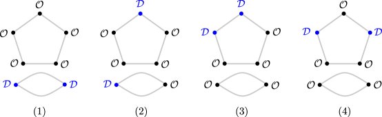
Figure 3.2: Diagrams for the integrand in the planar limit. The blue and black dots denote giant gravitons and single-trace operators, respectively. For each diagram, we need to take into account the permutations of $x_{1},x_{2}$ for the giant graviton and $x_{3},\ldots,x_{7}$ of the single-trace operators.

After imposing planarity, we still need to distinguish between giant gravitons and the single-trace operators. Taking into account the $S_{2}\times S_{5}$ symmetry, we find four in-equivalent diagrams as is shown in figure 3.2. The four diagrams correspond to the following polynomials

$$P_{1}^{(3)}(x_{i})=(x_{12}^{4})(x_{34}^{2}x_{45}^{2}x_{56}^{2}x_{67}^{2}x_{73}^{2})+S_{2}\times S_{5}\text{ permutations}\,,$$ (3.10)

$$P_{2}^{(3)}(x_{i})=(x_{13}^{4})(x_{24}^{2}x_{45}^{2}x_{56}^{2}x_{67}^{2}x_{72}^{2})+S_{2}\times S_{5}\text{ permutations}\,$$

$$P_{3}^{(3)}(x_{i})=(x_{67}^{4})(x_{12}^{2}x_{23}^{2}x_{34}^{2}x_{45}^{2}x_{51}^{2})+S_{2}\times S_{5}\text{ permutations}\,,$$

$$P_{4}^{(3)}(x_{i})=(x_{67}^{4})(x_{13}^{2}x_{32}^{2}x_{24}^{2}x_{45}^{2}x_{51}^{2})+S_{2}\times S_{5}\text{ permutations}\,.$$

The most general ansatz for the integrand is the linear combination of the above four polynomials

$$P^{(3)}(x_{i})=c_{1}\,P_{1}^{(3)}(x_{i})+c_{2}\,P_{2}^{(3)}(x_{i})+c_{3}\,P_{3}^{(3)}(x_{i})+c_{4}\,P_{4}^{(3)}(x_{i})$$ (3.11)

where $c_{1},\ldots,c_{4}$ are coefficients to be fixed.

3.3 The three-loop integral

To compute the correlation function we plug $P_{j}^{(3)}$ (3.10) into (3.8) and perform the integrals over $x_{5},x_{6},x_{7}$. It turns out that the resulting integrals can all be written in terms of the three-loop integrals that have appeared in the computation of the four-point function of 20’ operators. The definition of these integrals are summarized in appendix B. Let us denote the integrals

$$I_{j}^{(3)}\equiv x_{13}^{2}x_{24}^{2}\int\frac{P_{j}^{(3)}(x_{1},\ldots,x_{7})}{\prod_{1\leq p\leq 4\atop 5\leq q\leq 4+\ell}x_{pq}^{2}\prod_{5\leq p<q\leq 4+\ell}x_{pq}^{2}}\,\mathrm{d}^{4}x_{5}\mathrm{d}^{4}x_{6}\mathrm{d}^{4}x_{7}\,.$$ (3.12)

The four integrals can be written in terms of the known three-loop integrals as follows

$$I_{1}^{(3)}= \,6\left[gh(2,4;1,3)+gh(2,3;1,4)+gh(1,4;2,3)+gh(1,3;2,4)\right]$$ (3.13)

$$\,+6\left[L(2,4;1,3)+L(1,4;2,3)+L(2,3;1,4)+L(1,3;2,4)\right]$$

$$\,+6\left[E(1,2;3,4)+E(2,1;3,4)+E(1,3;2,4)+E(2,3;1,4)+E(1,4;2,3)+E(2,4;1,3)\right]$$

$$\,+6\left[T(1,4;2,3)+T(2,4;1,3)+T(1,3;2,4)+T(2,3;1,4)+T(1,2;3,4)+T(2,1;3,4)\right]\,,$$

$$I_{2}^{(3)}= \,6\left[gh(3,4;1,2)+L(3,4;1,2)\right]\,,$$

$$I_{3}^{(3)}= \,6\left[gh(1,2;3,4)+T(4,3;1,2)+T(3,4;1,2)\right]$$

$$\,+6\left[E(4,1;2,3)+E(3,1;2,4)+E(4,2;1,3)+E(3,2;1,4)\right]$$

$$\,+3\left[H(1,4;3,2)+H(2,4;3,1)+H(1,3;4,2)+H(2,3;4,1)\right]$$

$$\,+3\left[H(3,4;1,2)+H(3,4;2,1)\right]\,,$$

$$I_{4}^{(3)}= \,6\left[L(1,2;3,4)+T(4,1;2,3)+T(4,2;1,3)\right]$$

$$\,+6\left[T(3,1;2,4)+T(3,2;1,4)+E(4,3;1,2)+E(3,4;1,2)\right]$$

$$\,+3\left[H(1,2;3,4)+H(1,2;4,3)+H(1,4;2,3)\right]$$

$$\,+3\left[H(2,4;1,3)+H(1,3;2,4)+H(2,3;1,4)\right]\,.$$

Our final result is given by the linear combination of these integrals

$$\frac{G_{\{2,2\}}^{(3)}}{\tilde{R}_{1234}(d_{12})^{N-2}}=c_{1}\,I_{1}^{(3)}+c_{2}\,I_{2}^{(3)}+c_{3}\,I_{3}^{(3)}+c_{4}\,I_{4}^{(3)}\,$$ (3.14)

where $\tilde{R}_{1234}=R_{1234}/(x_{13}^{2}x_{24}^{2})$. To fix the four unknown coefficients, we need extra input. In the case of single-trace operators, one powerful constraint comes from the light-like limit where one can apply the duality between correlation functions and amplitudes Alday:2010zy ; Eden:2010zz . In the presence of the giant gravitons, we are not aware of such dualities. Therefore we need other means to fix these coefficients. In the next section we shall consider the OPE limit of the four-point functions in two different channels, which allows us to fix these coefficients. After obtaining the explicit result, we can then take the light-like limit of the four-point function. We find that, interestingly, the result (normalized by the Born level four-point function) is again the 3-loop four-point gluon MHV amplitude. This hints that the correlator/amplitude duality still holds in the presence of giant gravitons. For more details and discussions, we refer to section 4.3.

4 OPE limit

In the OPE limit, the leading contributions are controlled by a few conformal data such as the anomalous dimensions and OPE coefficients of low lying operators. It turns out to fix the four coefficients of the three-loop ansatz, it is sufficient to plug in two-loop conformal data for the low lying operators, which are already known in the literature. Because we have two kinds of operators $\mathcal{D}(x_{i})$ and $\mathcal{O}(x_{j})$, we also have two different OPE channels, which we shall call the $s$- and $t$-channel OPEs, as is shown in figure 4.3.

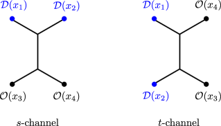
Figure 4.3: OPE in two different channels.

4.1 OPE in the $s$-channel

The $s$-channel OPE limit is defined by $x_{1}\to x_{2}$ and $x_{3}\to x_{4}$. In terms of conformal cross ratios, this corresponds to $u\rightarrow 0$ and $v\rightarrow 1$. In this limit, we replace the product $\mathcal{O}(x_{3})\mathcal{O}(x_{4})$ by the following series of operators,

$$\mathcal{O}(x_{3})\mathcal{O}(x_{4})= \,\mathsf{c}_{\mathcal{I}}\frac{(Y_{3}\cdot Y_{4})^{2}}{(x_{34}^{2})^{2}}\mathcal{I}+\mathsf{c}_{\mathcal{O}}\frac{(Y_{3}\cdot Y_{4})}{x_{34}^{2}}Y_{3I}Y_{4J}\mathcal{O}_{\mathbf{20^{\prime}}}^{IJ}(x_{4})$$ (4.1)

$$\,+\mathsf{c}_{\mathcal{K}}(g)\frac{(Y_{3}\cdot Y_{4})^{2}}{(x_{34}^{2})^{1-\delta\Delta_{\mathcal{K}}/2}}\mathcal{K}(x_{4})+\ldots,$$

where $\mathcal{I}$ is the identity operator, $\mathcal{K}$ is the Konishi operator, and $\mathcal{O}^{IJ}_{\mathbf{20^{\prime}}}$ belongs to the $\mathbf{20^{\prime}}$ representation of $SU(4)$. The conformal data of these operators control the leading and subleading contributions in the OPE limit $x_{3}\to x_{4}$. Since $\mathcal{O}_{\mathbf{20^{\prime}}}^{IJ}$ is a half-BPS operator, its anomalous dimension vanishes and $c_{\mathcal{O}}$ doesn’t depend on the coupling. Therefore the only coupling dependence comes from anomalous dimension and OPE coefficient of Konishi operator.

Similarly, we can perform the OPE of $\mathcal{D}(x_{1})\mathcal{D}(x_{2})$

$$\mathcal{D}(x_{1})\mathcal{D}(x_{2})= \,\mathsf{d}_{\mathcal{I}}\frac{(Y_{1}\cdot Y_{2})^{N}}{(x_{12}^{2})^{N}}+\mathsf{d}_{\mathcal{O}}\frac{(Y_{1}\cdot Y_{2})^{N-1}}{(x_{12}^{2})^{N-1}}Y_{3I}Y_{4J}\mathcal{O}_{\mathbf{20^{\prime}}}^{IJ}(x_{4})$$ (4.2)

$$\,+\mathsf{d}_{\mathcal{K}}(g)\frac{(Y_{1}\cdot Y_{2})^{N}}{(x_{12}^{2})^{N-1-\delta\Delta_{\mathcal{K}}/2}}\mathcal{K}(x_{2})+\ldots$$

Again the coupling dependence comes from the OPE data of Konish operator. We insert the OPEs (4.1) and (4.2) into the four-point function and expand up to three-loop order, leading to

$$\lim_{x_{1}\to x_{2}\atop x_{3}\rightarrow x_{4}}G_{\{2,2\}}^{(3)}=\left.\mathsf{d}_{\mathcal{K}}(g)\mathsf{c}_{\mathcal{K}}(g)\frac{(Y_{1}\cdot Y_{2})^{N}(Y_{3}\cdot Y_{4})^{2}}{(x_{12}^{2})^{N-1-\delta\Delta_{\mathcal{K}}/2}(x_{34}^{2})^{1-\delta\Delta_{\mathcal{K}}/2}}\left\langle\mathcal{K}(x_{2})\mathcal{K}(x_{4})\right\rangle\right|_{O(g^{6})}+\cdots\,,$$ (4.3)

where we normalize the two-point function of Konishi operator to be

$$\left\langle\mathcal{K}(x_{2})\mathcal{K}(x_{4})\right\rangle=\frac{1}{(x_{24}^{2})^{2+\delta\Delta_{\mathcal{K}}}}\,.$$ (4.4)

Plugging (4.4) into (4.3), we find that

$$\lim_{x_{1}\to x_{2}\atop x_{3}\rightarrow x_{4}}G_{\{2,2\}}^{(3)}=\left.\frac{y_{12}^{4}y_{34}^{4}}{x_{12}^{2}x_{34}^{2}x_{24}^{4}}(d_{12})^{N-2}\mathsf{d}_{\mathcal{K}}(g)\mathsf{c}_{\mathcal{K}}(g){u^{\delta\Delta_{\mathcal{K}}/2}}\right|_{O(g^{6})}\,.$$ (4.5)

The anomalous dimension of the Konishi operator and OPE coefficients can be expanded perturbatively

$$\delta\Delta_{\mathcal{K}}(g)= \,g^{2}\,\gamma_{1}+g^{4}\,\gamma_{2}+g^{6}\,\gamma_{3}+\cdots,$$ (4.6)

$$\mathsf{d}_{\mathcal{K}}(g)\mathsf{c}_{\mathcal{K}}(g)= \,C_{0}+g^{2}\,C_{1}+g^{4}\,C_{2}+g^{6}\,C_{3}+\cdots\,.$$

The coupling dependent part (4.5) thus can be expanded as

$$\left.\mathsf{d}_{\mathcal{K}}(g)\mathsf{c}_{\mathcal{K}}(g){u^{\delta\Delta_{\mathcal{K}}/2}}\right|_{O(g^{6})}= \,\frac{1}{48}C_{0}\,\gamma_{1}^{3}\,(\ln u)^{3}+\frac{1}{8}\left(C_{1}\,\gamma_{1}^{2}+2C_{0}\,\gamma_{1}\gamma_{2}\right)(\ln u)^{2}$$ (4.7)

$$\,+\frac{1}{2}\left(C_{0}\,\gamma_{3}+C_{1}\,\gamma_{2}+C_{2}\,\gamma_{1}\right)(\ln u)+C_{3}\,.$$

We notice that the result can be organized as a polynomial in $\ln u$. This structure plays an important role in our analysis below. In the expansion (4.7), the anomalous dimension of the Konishi operator and other twist-2 operators can be computed effectively by quantum spectral curve Gromov:2013pga up to very high orders (see for example Marboe:2014sya and references therein), so $\gamma_{n}$ is known. In addition, the coefficients $C_{k}$ contain the perturbative expansions of both $\mathsf{d}_{\mathcal{K}}(g)$ and $\mathsf{c}_{\mathcal{K}}(g)$. The result for $\mathsf{c}_{\mathcal{K}}(g)$ can be computed by the hexagon approach Basso:2015zoa and is known and checked up to 5-loop order Basso:2022nny ; Georgoudis:2017meq . The perturbative expansion of $\mathsf{d}_{\mathcal{K}}(g)$ can be computed by the $g$-function approach and has been tested up to two-loop order. To sum up, apart from $C_{3}$, we know all the other coefficients in the expansion (4.7).

$s$-channel OPE from the 3-loop ansatz

Now let us take the $s$-channel OPE limit of the 3-loop ansatz (3.14). We can use the symmetry of the integrals listed in appendix B to simplify the ansatz (3.14) and write the results in terms of the three-loop conformal integrals

$$\frac{G_{\{2,2\}}^{(3)}}{\tilde{R}_{1234}(d_{12})^{N-2}}= \,12(c_{1}+c_{4}){E(1,2;3,4)}+12(c_{1}+c_{3})[{E(1,3;2,4)}+{E(1,4;2,3)}]$$ (4.8)

$$\,+12(2c_{1}+c_{2}+2c_{3}+c_{4}){L(1,2;3,4)}$$

$$\,+12(2c_{1}+c_{4})[{L(1,3;2,4)}+{L(1,4;2,3)}]$$

$$\,+6(c_{2}+c_{3}){gh(1,2;3,4)}+12c_{1}[{gh(1,3;2,4)}+{gh(1,4;2,3)}]$$

$$\,+3(c_{3}+c_{4})(1+1/v){H(1,2;3,4)}+6(c_{4}+c_{3}\,u/v){H(1,3;2,4)}$$

$$\,+6(c_{4}+c_{3}\,u){H(1,4;2,3)}$$

The result for the integrals (4.8) in the $s$-channel OPE limit can be computed and are given in appendix B. Substitute the $s$-channel asymptotic results in (4.8), we obtain

$$\frac{G_{\{2,2\}}^{(3)}}{\tilde{R}_{1234}(d_{12})^{N-2}}= \,\frac{3}{16}(2c_{1}+c_{4})(\ln u)^{3}-\frac{3}{16}(19c_{1}+11c_{4})(\ln u)^{2}$$ (4.9)

$$\,+\frac{3}{8}\left[(37c_{1}+24c_{4})+3(2c_{1}+3c_{3}+c_{4})\zeta_{3}\right]\ln u$$

$$\,-\frac{9}{8}(19c_{1}+13c_{4})-\frac{3}{8}(9c_{1}+15c_{3}-8c_{4})\zeta_{3}$$

$$\,-\frac{15}{8}(4c_{1}+c_{2}+2c_{3}+3c_{4})\zeta_{5}$$

We can now compare (4.5) and (4.9). As we already discussed before, the coefficients of $(\ln u)^{n}$ with $n\geq 1$ contain only lower loop data. The constant term is our 3-loop prediction. In this way, we obtain 3 equations, corresponding to the 3 coefficients in front of $(\ln u)^{n}$ with $n=1,2,3$:

$$24c_{1}+12c_{4}= \,\frac{1}{48}C_{0}\gamma_{1}^{3}\,,$$ (4.10)

$$-228c_{1}-132c_{4}= \,\frac{1}{8}(C_{1}\gamma_{1}^{2}+2C_{0}\gamma_{1}\gamma_{2})\,,$$

$$888c_{1}+576c_{4}+72(2c_{1}+3c_{2}+c_{4})\zeta(3)= \,\frac{1}{2}\left(C_{0}\gamma_{3}+C_{1}\gamma_{2}+C_{2}\gamma_{1}\right)\,.$$

Plugging in the following perturbative data up to two-loops

$$\delta\Delta_{\mathcal{K}}(g)= \,\gamma_{1}\,g^{2}+\gamma_{2}\,g^{4}+\gamma_{3}\,g^{6}+\cdots=12g^{2}-48g^{4}+336g^{6}+\cdots\,,$$ (4.11)

$$\mathsf{d}_{\mathcal{K}}(g)\mathsf{c}_{\mathcal{K}}(g)= \,C_{0}+C_{1}\,g^{2}+C_{2}\,g^{4}+\cdots=\frac{1}{3}-4g^{2}+56g^{4}+\cdots\,,$$

we find the following simple solution

$$c_{1}=\frac{1}{3},\qquad c_{2}=-\frac{1}{3},\qquad c_{4}=\frac{1}{3}\,.$$ (4.12)

Therefore the $s$-channel OPE alone fixes 3 out of 4 unknown coefficients. To obtain $c_{3}$, we need to consider the $t$-channel OPE.

4.2 OPE in the $t$-channel

Now we consider the $t$-channel OPE limit $x_{1}\rightarrow x_{4}$ and $x_{2}\rightarrow x_{3}$, which is equivalently to $u\rightarrow 1$ and $v\rightarrow 0$. In this channel, the dominant contribution comes from an operator with dimension $N+\delta\Delta_{\text{open}}(g)$ where $N$ is the bare dimension. We have the following OPE

$$\mathcal{D}(x_{1})\mathcal{O}(x_{4})=\mathsf{c}_{\mathcal{O}\text{open}}(g)\frac{(Y_{1}\cdot Y_{4})^{2}}{(x_{14}^{2})^{1-\delta\Delta_{\text{open}}/2}}\mathcal{O}_{\text{open}}+\cdots$$ (4.13)

To have the correct harmonic charge and bare dimension, the candidate operator should take the form

$$\mathcal{O}_{\text{open}}\sim\epsilon^{j_{1}...j_{N-2}a_{1}a_{2}}_{i_{1}...i_{N-2}b_{1}b_{2}}(\mathcal{Z}_{1})^{i_{1}}_{j_{1}}\cdots(\mathcal{Z}_{1})^{i_{N-2}}_{j_{N-2}}(\Phi_{I})_{b_{1}}^{a_{1}}(\Phi_{I})_{b_{2}}^{a_{2}}.$$ (4.14)

where $\mathcal{Z}_{1}=Y_{1}^{I}\Phi_{I}$ and we sum over $I=1,\ldots,6$ for the last two scalar fields. This is not a familiar operator of the $Z=0$ or $Y=0$ brane excitations. In Jiang:2019xdz it was conjectured that $\mathcal{O}_{\text{open}}$ corresponds to the $Z=0$ brane with length-1 excitation. This does not seem to be the case. However, in fact we do not have to make further assumptions about this operator, the CFT data $\mathsf{c}_{\mathcal{O}\text{open}}(g)$ and $\delta\Delta_{\text{open}}(g)$ can be fixed up to two-loop order solely from lower loop data. We give the main idea here and the details can be found in appendix A. Let us denote the perturbative expansion of the OPE data as

$$(\mathsf{c}_{\mathcal{O}\text{open}}(g))^{2}= \,\widetilde{C}_{0}+\widetilde{C}_{1}\,g^{2}+\widetilde{C}_{2}\,g^{4}+\widetilde{C}_{3}\,g^{6}+\cdots$$ (4.15)

$$\delta\Delta_{\text{open}}(g)= \,\tilde{\gamma}_{1}\,g^{2}+\tilde{\gamma}_{2}\,g^{4}+\tilde{\gamma}_{3}\,g^{6}+\cdots$$

where $\widetilde{C}_{0}$ can be fixed easily from a Born level computation. At one-loop, there is only one unknown coefficient, which can be fixed by the $s$-channel OPE. This gives us the full one-loop answer. By performing a $t$-channel OPE, we can extract $\mathsf{c}_{\mathcal{O}\text{open}}(g)$ and $\delta\Delta_{\text{open}}(g)$ up to one-loop. At two-loop, there are two unknown coefficients, one of which can be fixed by the $s$-channel OPE. The other one can be fixed by $t$-channel OPE. It turns out that there are several equations in the $t$-channel OPE, one of them involve only lower order OPE data $\widetilde{C}_{0}$, $\widetilde{C}_{1}$ and $\tilde{\gamma}_{1}$, which have been determined in the previous step. We can use this equation to fix the second unknown coefficient, which then give us the full two-loop result. Performing the $t$-channel OPE, we can extract $\widetilde{C}_{2}$ and $\tilde{\gamma}_{2}$. This procedure leads to the following result

$$(\mathsf{c}_{\mathcal{O}\text{open}}(g))^{2}= \,1-4g^{2}+24(1+\zeta_{3})g^{4}+\cdots,$$ (4.16)

$$\delta\Delta_{\text{open}}(g)= \,4g^{2}-8g^{4}+\cdots\,.$$

Using the $t$-channel OPE (4.13) and a similar one for $\mathcal{D}(x_{2})$ and $\mathcal{O}(x_{3})$, we obtain the correlator in the OPE limit

$$\lim_{x_{4}\to x_{1}\atop x_{3}\to x_{2}}G_{\{2,2\}}^{(3)}=\left.{(\mathsf{c}_{\mathcal{O}\text{open}})^{2}}\frac{(Y_{1}\cdot Y_{4})^{2}(Y_{2}\cdot Y_{3})^{2}}{(x_{14}^{2})^{1-\delta\Delta_{\text{open}}/2}(x_{23}^{2})^{1-\delta\Delta_{\text{open}}/2}}\langle\mathcal{O}_{\text{open}}(x_{1})\mathcal{O}_{\text{open}}(x_{2})\rangle\right|_{{O}(g^{6})}+\cdots$$ (4.17)

Using

$$\langle\mathcal{O}_{\text{open}}(x_{1})\mathcal{O}_{\text{open}}(x_{2})\rangle\propto\frac{d_{12}^{N-2}}{(x_{12}^{2})^{2+\delta\Delta_{\text{open}}}}\,,$$ (4.18)

we obtain

$$\lim_{x_{4}\to x_{1}\atop x_{3}\to x_{2}}G_{\{2,2\}}^{(3)}=\left.{(\mathsf{c}_{\mathcal{O}\text{open}})^{2}}\frac{y_{14}^{4}y_{23}^{4}}{x_{14}^{2}x_{23}^{2}x_{12}^{4}}v^{\delta\Delta_{\text{open}}/2}\right|_{{O}(g^{6})}$$ (4.19)

We have the following perturbative expansion

$$\left.\left(\mathsf{c}_{\mathcal{O}\text{open}}(g)\right)^{2}{v^{\delta\Delta_{\text{open}}/2}}\right|_{O(g^{6})}= \,\frac{1}{48}\widetilde{C}_{0}\,\tilde{\gamma}_{1}^{3}\,(\ln v)^{3}+\frac{1}{8}\left(\widetilde{C}_{1}\,\tilde{\gamma}_{1}^{2}+2\widetilde{C}_{0}\,\tilde{\gamma}_{1}\tilde{\gamma}_{2}\right)(\ln v)^{2}$$ (4.20)

$$\,+\frac{1}{2}\left(\widetilde{C}_{0}\,\tilde{\gamma}_{3}+\widetilde{C}_{1}\,\tilde{\gamma}_{2}+\widetilde{C}_{2}\,\tilde{\gamma}_{1}\right)(\ln v)+\widetilde{C}_{3}\,.$$

On the other hand, we can take the $t$-channel OPE limit in our ansatz (4.8) using the results of the three-loop integrals in the $t$-channel OPE limit, which leads to

$$\lim_{x_{4}\to x_{1}\atop x_{3}\to x_{2}}\frac{G_{\{2,2\}}^{(3)}}{\tilde{R}_{1234}(d_{12})^{N-2}}= \,\frac{1}{16}(4c_{1}+c_{2}+3c_{3}+c_{4})(\ln v)^{3}$$ (4.21)

$$\,-\frac{3}{16}(13c_{1}+3c_{2}+10c_{3}+4c_{4})(\ln v)^{2}$$

$$\,+\frac{3}{32}\left[(104c_{1}+22c_{2}+79c_{3}+39c_{4})+24(c_{1}+c_{3}+c_{4})\zeta(3)\right](\ln v)$$

$$\,-\frac{3}{16}(82c_{1}+16c_{2}+57c_{3}+37c_{4})-\frac{3}{8}(9c_{1}+7c_{4})\zeta(3)$$

$$\,-\frac{15}{4}(3c_{1}+c_{3}+c_{4})\zeta(5)$$

Collecting the coefficients of $(\ln v)^{n}$ with $n\geq 1$ and comparing with (4.20), we obtain the following equations

$$16c_{1}+4c_{2}+12c_{3}+4c_{4}= \,\frac{1}{48}\widetilde{C}_{0}\,\tilde{\gamma}_{1}^{3}\,,$$ (4.22)

$$-156c_{1}-36c_{2}-120c_{3}-48c_{4}= \,\frac{1}{8}\left(\widetilde{C}_{1}\,\tilde{\gamma}_{1}^{2}+2\widetilde{C}_{0}\,\tilde{\gamma}_{1}\tilde{\gamma}_{2}\right)\,,$$

$$6(104c_{1}+22c_{2}+79c_{3}+39c_{4})+144(c_{1}+c_{3}+c_{4})\zeta_{3}= \,\frac{1}{2}\left(\widetilde{C}_{0}\,\tilde{\gamma}_{3}+\widetilde{C}_{1}\,\tilde{\gamma}_{2}+\widetilde{C}_{2}\,\tilde{\gamma}_{1}\right)\,.$$

Since we only need to determine $c_{3}$, it is sufficient to consider the first equation in (4.22). Plugging in the perturbative data (4.16) and the solution from $s$-channel (4.12), we find that

$$c_{3}=-\frac{1}{3}\,.$$ (4.23)

We can then use the second equation of (4.22) as a consistency check, which is indeed satisfied. Plugging the solutions into (4.8), we obtain

$$\frac{G^{(3)}_{\{2,2\}}}{\tilde{R}_{1234}(d_{12})^{N-2}}= \,4\left[gh(1,3;2,4)+gh(1,4;2,3)-gh(1,2;3,4)\right]$$ (4.24)

$$\,+12\left[L(1,3;2,4)+L(1,4;2,3)\right]+8E(1,2;3,4)$$

$$\,+2\left(1-\frac{u}{v}\right)H(1,3;2,4)+2(1-u)H(1,4;2,3)\,.$$

This is the main result of the current work. We note that it is similar to the three-loop result of four single-trace operators, but somewhat simpler. Not all the three-loop integrals appear.

4.3 Light-like limit

In this subsection, we consider the light-like limit $x_{i,i+1}^{2}\to 0$ of the four-point function $G_{\{2,2\}}/G_{\{2,2\}}^{(0)}$ with $n=1,2,3$. In the case of four BPS single-trace operators of length-2, this quantity corresponds to the square of the four-gluon MHV amplitude. This fact was called the correlator/amplitude duality Alday:2010zy ; Eden:2010zz . We shall find that this duality still holds in the presence of giant gravitons.

Tree level

The tree-level result reads Jiang:2019xdz ; Jiang:2019zig

$$\frac{G_{\{2,2\}}^{(0)}}{(d_{12})^{N}(d_{34})^{2}}=\frac{z\bar{z}}{\alpha\bar{\alpha}}\left[\frac{(1-\alpha)(1-\bar{\alpha})}{(1-z)(1-\bar{z})}+1\right]-2\left(\frac{z\bar{z}}{\alpha\bar{\alpha}}\right)^{2}\frac{(1-\alpha)(1-\bar{\alpha})}{(1-z)(1-\bar{z})}\,.$$ (4.25)

In the light-like limit $x_{i,i+1}^{2}\to 0$, we have

$$z\bar{z}=\frac{x_{12}^{2}x_{34}^{2}}{x_{13}^{2}x_{24}^{2}}\to 0,\qquad(1-z)(1-\bar{z})=\frac{x_{14}^{2}x_{23}^{2}}{x_{13}^{2}x_{24}^{2}}\to 0$$ (4.26)

Keeping the leading term in this limit, we find that

$$G_{\{2,2\}}^{(0)}\sim(d_{12})^{N}(d_{34})^{2}\frac{z\bar{z}}{\alpha\bar{\alpha}}\frac{(1-\alpha)(1-\bar{\alpha})}{(1-z)(1-\bar{z})}=\frac{x_{12}^{2}x_{34}^{2}}{x_{14}^{2}x_{23}^{2}}\frac{y_{14}^{2}y_{23}^{2}}{y_{12}^{2}y_{34}^{2}}\,(d_{12})^{N}(d_{34})^{2}$$ (4.27)

At loop level, the global factor $\tilde{R}_{1234}(d_{12})^{N-2}$ in the light-like limit becomes

$$\frac{R_{1234}}{x_{13}^{2}x_{24}^{2}}(d_{12})^{N-2}\sim\frac{y_{12}^{2}y_{23}^{2}y_{34}^{2}y_{14}^{2}}{x_{12}^{2}x_{23}^{2}x_{34}^{2}x_{14}^{2}}(d_{12})^{N-2}=\frac{y_{23}^{2}y_{14}^{2}}{x_{23}^{2}x_{14}^{2}}\frac{x_{12}^{2}x_{34}^{2}}{y_{12}^{2}y_{34}^{2}}(d_{12})^{N}(d_{34})^{2}\,.$$ (4.28)

which is cancelled precisely by dividing $G_{\{2,2\}}^{(0)}$.

One-loop

At one-loop level, we have

$$\lim_{x_{i,i+1}^{2}\to 0}\frac{G_{\{2,2\}}^{(1)}}{G_{\{2,2\}}^{(0)}}=2g(1,2,3,4)\,.$$ (4.29)

Two-loop

At two-loop, we have

$$\lim_{x_{i,i+1}^{2}\to 0}\frac{G_{\{2,2\}}^{(2)}}{G_{\{2,2\}}^{(0)}}=2h(1,3;2,4)+2h(2,4;1,3)+g(1,2,3,4)^{2}$$ (4.30)

Three-loop

At three-loop, we have

$$\lim_{x_{i,i+1}^{2}\to 0}\frac{G_{\{2,2\}}^{(3)}}{G_{\{2,2\}}^{(0)}}= \,2gh(1,3;2,4)+2gh(2,4;1,3)$$ (4.31)

$$\,+2L(2,4;1,3)+2L(1,3;2,4)+2T(2,4;1,3)$$

$$\,+2T(1,3;2,4)+2T(4,2;1,3)+2T(3,1;2,4)\,.$$

Noticing that in taking the light-like limit, some of the integral identities do not hold anymore. For example, the $T$-integrals do not equal to $L$-integrals in this limit. On the other hand, the four-gluon MHV amplitude up to three-loop order is given byDrummond:2006rz Anastasiou:2003kj

$$\frac{\mathcal{A}}{\mathcal{A}^{(0)}}= \,1+g^{2}\,[g(1,2,3,4]+g^{4}[h(1,3;2,4)+h(2,4;1,3)]$$ (4.32)

$$\,+g^{6}[T(1,3;2,4)+T(3,1;2,4)+T(2,4;1,3)+T(4,2;1,3)$$

$$\,\quad+L(1,3;2,4)+L(2,4;1,3)]\,.$$

From these explicit results, we find that up to three-loop order

$$\lim_{x_{i,i+1}^{2}\to 0}\frac{G_{\{2,2\}}}{G^{(0)}_{\{2,2\}}}=\left(\frac{\mathcal{A}}{\mathcal{A}^{(0)}}\right)^{2}+\mathcal{O}(g^{8})\,.$$ (4.33)

Therefore in the light-like limit, the four-point function is also the square of the MHV amplitude. It is natural to conjecture that this relation holds at higher-loop orders, or even non-perturbatively.

If this were the case, we can use this relation to constrain the four-point functions with giant gravitons. However, we would like to point out that, this is only sufficient to fix part of the unknown coefficients both at two-loop and three-loops. These are the coefficients that can be fixed by the $s$-channel OPE limit. This is different from the case where the four-operators are length-2 BPS operators. The reason is that the latter has a larger permutation symmetry since the four single-trace operators are identical. Therefore we have fewer unknown coefficients, which can be fixed completely by the correlator/amplitude duality.

5 OPE data at three-loop order

From the explicit form of the four-point function, we can extract the OPE data up to this loop order. For length-2 single-trace BPS operators, at the leading OPE limit in the $s$-channel we can extract OPE data for twist-2 operators. There is no degeneracy for twist-2 operators and we have one operator for each spin. We denote the twist-2 operator with spin-$S$ by $\mathcal{O}_{S}$. The OPE coefficients of two giant gravitons and two length-$L$ half-BPS operators will be denoted by $\mathsf{d}_{S}$ and $\mathsf{c}_{LLS}$ respectively.

From our result (4.24), we can extract the product of OPE coefficients $\mathsf{d}_{S}\mathsf{c}_{22S}$ at three-loop order using the method described in Vieira:2013wya . The result is given in Table 1.

spin-$S$	$\mathsf{d}_{S}\mathsf{c}_{22S}|_{O(g^{6})}$
2	$-768+112\zeta_{3}-160\zeta_{5}$
4	$-\frac{442765625}{3500658}+\frac{386}{27}\zeta_{3}-\frac{400}{21}\zeta_{5}$
6	$-\frac{1183056555847}{88944075000}+\frac{48286}{37125}\zeta_{3}-\frac{56}{33}\zeta_{5}$
8	$-\frac{1270649655622342732745039}{1075922954067591630000000}+\frac{1039202363}{9932422500}\zeta_{3}-\frac{6088}{45045}\zeta_{5}$
10	$-\frac{7465848687069712820911408164847}{77747563297936585275804036000000}+\frac{8295615163}{1049947353000}\zeta_{3}-\frac{2684}{264537}\zeta_{5}$

Table 1: 3-loop result of the OPE coefficient from spin 2 to 10.

Dividing the result by the known results of $\mathsf{c}_{22S}$ and taking the square, we find the OPE coefficient $(\mathsf{d}_{S})^{2}$. The results up to $S=10$ are given below

$$\mathsf{d}_{2}^{2}= \,\frac{1}{3}-4g^{2}+(56-24\zeta_{3})g^{4}+16(22\zeta_{3}+5\zeta_{5}-48)g^{6}\,,$$ (5.1)

$$\mathsf{d}_{4}^{2}= \,\frac{1}{35}-\frac{205}{441}g^{2}+\left(\frac{70219}{9261}-\frac{20\zeta_{3}}{7}\right)g^{4}+\left(\frac{58868\zeta_{3}}{1323}+\frac{200\zeta_{5}}{21}-\frac{200151970}{1750329}\right)g^{6}\,,$$

$$\mathsf{d}_{6}^{2}= \,\frac{1}{462}-\frac{1106}{27225}g^{2}+\left(\frac{772465873}{1078110000}-\frac{14\zeta_{3}}{55}\right)g^{4}+\left(\frac{316477\zeta_{3}}{81675}+\frac{28\zeta_{5}}{33}-\frac{1001837354497}{88944075000}\right)g^{6}\,,$$

$$\mathsf{d}_{8}^{2}= \,\frac{1}{6435}-\frac{14380057}{4509004500}g^{2}+\left(\frac{5048546158688587}{85305405235050000}-\frac{1522\zeta_{3}}{75075}\right)g^{4}$$

$$+\left(\frac{209601639281\zeta_{3}}{710168208750}+\frac{3044\zeta_{5}}{45045}-\frac{256288425994027633489541}{268980738516897907500000}\right)g^{6}\,,$$

$$\mathsf{d}^{2}_{10}= \,\frac{1}{92378}-\frac{3313402433}{13995964873800}g^{2}+\left(\frac{141793274806850941159}{31100584702491617040000}-\frac{671\zeta_{3}}{440895}\right)g^{4}$$

$$+\left(\frac{11578996460944\zeta_{3}}{551091116905875}+\frac{1342\zeta_{5}}{264537}-\frac{5796660491433231307517026775347}{77747563297936585275804036000000}\right)g^{6}$$

5.1 Harmonic sum and large spin limit

In order to write down the result of $\mathsf{d}_{S}^{2}$ in a closed form for arbitrary spin $S$, we can rewrite the results in terms of nested harmonic sums.

Harmonic Sum

The harmonic sums are defined as

$$S_{a}(j)\equiv\left\{\begin{array}[]{ll}\sum_{n=1}^{j}\frac{1}{n^{|a|}}&a\geq 0\\ \sum_{n=1}^{j}\frac{(-1)^{n}}{n^{|a|}}&a<0\end{array},\quad S_{a,b,\ldots}(j)\equiv\begin{cases}\sum_{n=1}^{j}\frac{1}{n^{|a|}}S_{b,\ldots}(n)&a\geq 0\\ \sum_{n=1}^{j}\frac{(-1)^{n}}{n^{|a|}}S_{b,\ldots}(n)&a<0\end{cases}\right.$$ (5.2)

For simplicity, we will omit the argument of the harmonic sums in what follows. The main idea is to write down an ansatz for the result as a linear combination of harmonic sums with certain weights. In order to fix the coefficients, we calculate the structure constant up to sufficiently high spin. For a given weight, we can choose a basis for all the harmonic sums. For example, the basis at weight 6 contains 486 independent harmonic sums. Such a basis can be found with the aide of certain packages like HarmonicSumAblinger:2014rba . Once all the coefficients are fixed, its correctness can be tested by comparing with even higher spin results. At each loop order, we make the uniform transcendentality ansatz with transcendental degree $2n$ at $n$-loops. Such a procedure has been carried out up to two-loop Jiang:2019xdz . With our result, we can push this calculation to three loops, the result is given by

$$\left(\frac{\mathsf{d}_{j}}{\left.\mathsf{d}_{j}\right|_{\text{tree }}}\right)^{2}=\texttt{prefactor}\times\left[1-4g^{2}S_{2}+8g^{4}\left(d_{2,4}+d_{2,1}\zeta_{3}\right)+64g^{6}\left(d_{3,6}+d_{3,3}\zeta_{3}+d_{3,1}\zeta_{5}\right)\right],$$ (5.3)

with

$$d_{2,1}= \,-6S_{1}\,$$ (5.4)

$$d_{2,4}= \,5S_{-4}+8S_{-3}S_{1}+4S_{-2}\left(S_{1}\right)^{2}+2S_{-2}S_{2}+2\left(S_{2}\right)^{2}+8S_{1}S_{3}$$ (5.5)

$$+7S_{4}-8S_{-3,1}-8S_{1}S_{-2,1}-6S_{-2,2}-4S_{1,3}-4S_{3,1}+8S_{-2,1,1}\,$$

and

$$d_{3,1}= \,\frac{5}{2}S_{1}\,$$ (5.6)

$$d_{3,3}= \,-2S_{-2,1}-\frac{4S_{1}^{3}}{3}+6S_{2}S_{1}+S_{-3}+\frac{4S_{3}}{3},$$ (5.7)

$$d_{3,6}= \frac{4}{3}S_{1}^{3}S_{-2,1}+16S_{1}^{2}S_{-3,1}+10S_{1}^{2}S_{-2,2}-8S_{1}^{2}S_{-2,1,1}+31S_{1}S_{-4,1}+2S_{-2}S_{1}S_{-2,1}$$ (5.8)

$$-12S_{2}S_{1}S_{-2,1}-2S_{1}S_{-2,3}-4S_{1}S_{2,-3}+24S_{-2}S_{1}S_{2,1}-36S_{1}S_{-3,1,1}+4S_{1}S_{-2,1,-2}$$

$$-24S_{1}S_{-2,2,1}-24S_{1}S_{2,1,-2}+24S_{1}S_{-2,1,1,1}+2S_{-2,1}^{2}-8S_{-5,1}+17S_{-4,2}+2S_{-2}S_{-3,1}$$

$$-16S_{2}S_{-3,1}-3S_{-3,3}-2S_{-3}S_{-2,1}+\frac{38}{3}S_{3}S_{-2,1}+2S_{-2}S_{-2,2}+8S_{2}S_{-2,2}-6S_{-2}S_{3,1}$$

$$-21S_{4,-2}-4S_{-2}S_{-2,1,1}+16S_{2}S_{-2,1,1}-20S_{-2,2,2}+6S_{-2,3,1}+26S_{2,-3,1}+6S_{3,1,-2}$$

$$+40S_{-3,1,1,1}-28S_{2,-2,1,1}-32S_{-2,1,1,1,1}-\frac{14}{3}S_{-3}S_{1}^{3}-2S_{-2}^{2}S_{1}^{2}-17S_{-4}S_{1}^{2}-6S_{-2}S_{2}S_{1}^{2}$$

$$-3S_{4}S_{1}^{2}+\frac{7}{2}S_{-5}S_{1}-5S_{-3}S_{-2}S_{1}+14S_{-3}S_{2}S_{1}-8S_{-2}S_{3}S_{1}-6S_{2}S_{3}S_{1}-\frac{17S_{5}S_{1}}{2}$$

$$-S_{2}^{3}+\frac{S_{-3}^{2}}{2}-2S_{-2}S_{2}^{2}-S_{3}^{2}+4S_{-6}-S_{-4}S_{-2}-\frac{1}{2}S_{-2}^{2}S_{2}-\frac{13}{2}S_{-4}S_{2}-\frac{34}{3}S_{-3}S_{3}$$

$$+18S_{-2}S_{4}-3S_{2}S_{4}-\frac{5S_{6}}{2}.$$

The prefactor is given by

$$\texttt{prefactor}=\frac{\Gamma(2j+1)\Gamma\left(j+\frac{\gamma}{2}+1\right)^{2}}{\Gamma(j+1)^{2}\Gamma(2j+\gamma+1)}-\frac{1}{4}\left(-\gamma^{2}+(S_{1}(2j)-S_{1}(j))\gamma^{3}\right)\zeta_{2}-\frac{\gamma^{3}\zeta_{3}}{4},$$ (5.9)

where $\gamma=\delta\Delta_{\mathcal{K}}$ is anomalous dimension.

Large Spin Limit

Another advantage of the harmonic sum representation is that it allows us to make analytic continuation and extract the large spin behavior of the structure constant. The details are delegated to appendix C. Here we simply present the final answer at leading order:

$$\ln\left[\left(\frac{\mathsf{d}_{j}}{\left.\mathsf{d}_{j}\right|_{\text{tree }}}\right)^{2}\right]= -4g^{2}\Big{(}\zeta_{2}+2\ln{2}\ln{S}\Big{)}+\frac{8}{5}g^{4}\Big{(}8\zeta_{2}^{2}+15\zeta_{3}\ln{2}+10\zeta_{2}\ln{2}\ln{S}-15\zeta_{3}\ln{S}\Big{)}$$ (5.10)

$$+\frac{16}{105}g^{6}\Big{(}-449\zeta_{2}^{3}+385\zeta_{3}^{2}-210\zeta_{2}\zeta_{3}\ln{2}-1050\zeta_{5}\ln{2}$$

$$-462\zeta_{2}^{2}\ln{2}\ln{S}+420\zeta_{2}\zeta_{3}\ln{S}+1050\zeta_{5}\ln{S}$$

$$-252\zeta_{2}^{2}(\ln{S})^{2}+840\zeta_{2}\ln{2}(\ln{S})^{3}-280\zeta_{3}(\ln{S})^{3}\Big{)},$$

where $\ln{S}=\ln{j}+\gamma_{E}$ and $\gamma_{E}$ is the Euler constant. Up to two-loop, the large spin limit exhibit only $\ln S$ behavior. However, as we can see from the result, at three-loop order we start to have contributions like $(\ln S)^{2}$ and $(\ln S)^{3}$.

5.2 Discussions

Intriguingly, we find that up to three-loop order, our results of $\mathsf{d}_{S}\mathsf{c}_{22S}$ in Table 1 coincide exactly with $\mathsf{c}_{44S}^{2}$ (see e.g. Table-1 of Basso:2015eqa ).

$$\mathsf{d}_{S}\mathsf{c}_{22S}=\mathsf{c}_{44S}^{2}$$ (5.11)

At three-loop order, we actually have

$$\mathsf{c}_{44S}^{2}=\mathsf{c}^{2}_{LLS},\qquad L\geq 4\,.$$ (5.12)

This is clear from the point of view of hexagon form factors. The OPE coefficients of $\mathsf{c}_{LLS}$ have the same asymptotic contribution and the adjacent wrapping contributions. What makes the difference is the bottom or opposite wrapping corrections. For $L\geq 4$, bottom wrappings do not contribute at three-loop order. However, for $L=2$ we do have non-zero three-loop contribution and we have

$$\mathsf{c}_{44S}^{2}=\mathsf{c}_{22S}^{2}-\texttt{bottom wrapping}$$ (5.13)

The relation (5.11) shows that there is an intimate relation between the OPE coeffcients of single trace operators and giant gravitons with twist-two operators. It is tempting to conjecture that at higher loop orders, similar relation $\mathsf{d}_{S}\mathsf{c}_{22S}=\mathsf{c}_{LLS}^{2}$ holds for $L>4$. If this were the case, it implies that there should be an intimate connection between the worldsheet $g$-function approach and the hexagon form factor approach to the OPE coefficients. One can expect to use the $g$-function to partially resum the hexagon mirror corrections. This would be fascinating to check.

6 Conclusions and Outlook

In this paper, we computed the four-point function with two maximal giant gravitons and two length-2 single-trace chiral BPS operators up to three-loop order in the planar limit. Our main result is (4.24) written in terms of known three-loop conformal integrals. From the four-point function, we extract the OPE coefficients of two giant graviton and twist-two operators with arbitrary spin. The result is given in terms of harmonic sums (5.3), from which we can extract the large spin behavior of the OPE coefficient. We find the contributions of the form $(\ln S)^{2}$ and $(\ln S)^{3}$ start to contribute at three-loop order.

From the explicit results, we find an intriguingly simple relation between the OPE coefficient of giant gravitons and single-trace operators, given in (5.11). This relation hints a deep connection between these two types of OPE coefficients. From integrability point of view, these two kinds of OPE coefficients are computed by different approaches. The giant graviton OPE coefficient is computed by the worldsheet $g$-function approach. The advantage of this approach is that all the finite size corrections can be taken into account, thanks to thermodynamic Bethe ansatz. On the other hand, the OPE coefficient of single-trace operators are computed by hexagon form factors. A systematic approach to take into account all finite size corrections is still missing at the moment, although important partial progress has been made (see for example Jiang:2016ulr ; Kostov:2019stn ; Belitsky:2020qrm ; Bargheer:2019kxb ; Bargheer:2019exp ). In particular, there is an all-loop conjecture for the OPE coefficients $\mathsf{c}_{22S}$ Basso:2022nny . It would be interesting to make a more explicit connection between these two approaches.

There are many future questions that need to be addressed. The first thing would be test the $g$-function prediction from integrability using our field theoretical result. In particular, we will see whether some kind of wrapping corrections would show up at this loop order, or asymptotic result is sufficient like in the spectral problem. This work has been initiated and we would like to report it elsewhere.

Another important direction is to extent the field theoretical result to include BPS operators with larger length, namely compute the four-point functions of $\langle\mathcal{D}(x_{1})\mathcal{D}(x_{2})\mathcal{O}_{j}(x_{3})\mathcal{O}_{k}(x_{4})\rangle$ for $j,k>2$ up to three-loop order. At the same time, it is also interesting to consider four-point functions of giant gravitons, namely $\langle\mathcal{D}(x_{1})\ldots\mathcal{D}(x_{4})\rangle$. Such correlation functions is only known up to one-loop, but we believe it should be possible to push it to at least three-loop orders.

Finally a more challenging but obvious next step is to compute all the aforementioned four-point functions to 4- and 5-loops, catching up with the results of the single-trace operators. However, the unknown coefficients grows rapidly. Our current strategy which uses lower loop data can only fix part of the unknown coefficients. To fix the full result, we shall need more constraints from other principles.

Appendix A Perturbative results up to two-loop

In this section, we review the results for the giant graviton two-point function up to two-loop order. We will compare the results in the $s$- and $t$-channels by direct computation and OPE analysis.

$s$-channel

In the $s$-channel direct computation, for the result written in terms an ansatz, we have

$$\lim_{z,\bar{z}\to 0}\frac{G_{\{2,2\}}^{(\ell)}}{\tilde{R}_{1234}(d_{12})^{N-2}}=\lim_{u\to 0\atop v\to 1}\frac{G_{\{2,2\}}^{(\ell)}}{\tilde{R}_{1234}(d_{12})^{N-2}}=\sum_{k}c_{k}\,\lim_{u\to 0\atop v\to 1}I^{(l)}_{k}$$ (A.1)

where we take the proper limit for the conformal integrals at $\ell$-loop order. On the other hand, from OPE analysis, we have

$$\lim_{x_{1}\to x_{2}\atop x_{3}\to x_{4}}\frac{G_{\{2,2\}}^{(\ell)}}{\tilde{R}_{1234}(d_{12})^{N-2}}=\left.\mathsf{d}_{\mathcal{K}}(g)\mathsf{c}_{\mathcal{K}}(g)u^{\delta\Delta/2}\right|_{O(g^{2\ell})}\,.$$ (A.2)

We make the following expansion

$$\delta\Delta(g)=\sum_{n=1}^{\infty}\gamma_{n}\,g^{2n},\qquad\mathsf{d}_{\mathcal{K}}(g)\mathsf{c}_{\mathcal{K}}(g)=\sum_{n=0}^{\infty}C_{n}\,g^{2n}$$ (A.3)

From tree level computation, we find that $C_{0}=1/3$. From integrability, $\gamma_{1}=12$.

$t$-channel

In the $t$-channel, from the ansatz we have

$$\lim_{z,\bar{z}\to 1}\frac{G_{\{2,2\}}^{(\ell)}}{\tilde{R}_{1234}(d_{12})^{N-2}}=\lim_{u\to 1\atop v\to 0}\frac{G_{\{2,2\}}^{(\ell)}}{\tilde{R}_{1234}(d_{12})^{N-2}}=\sum_{k}c_{k}\,\lim_{u\to 1\atop v\to 0}I^{(l)}_{k}$$ (A.4)

where again we need to take the proper limit of the conformal integral. From OPE analysis, we have

$$\lim_{x_{1}\to x_{4}\atop x_{3}\to x_{2}}\frac{G_{\{2,2\}}^{(\ell)}}{\tilde{R}_{1234}(d_{12})^{N-2}}=\left.(\mathsf{c}_{\mathcal{O}_{\text{open}}}(g))^{2}\,v^{\delta\Delta_{\text{open}}/2}\right|_{O(g^{2\ell})}\,.$$ (A.5)

We make the following expansion

$$\delta\Delta_{\text{open}}=\sum_{n=1}^{\infty}\tilde{\gamma}_{n}\,g^{2n},\qquad\left(\mathsf{c}_{\text{Open}}(g)\right)^{2}=\sum_{n=0}^{\infty}\widetilde{C}_{n}g^{2n}\,.$$ (A.6)

From tree level computation, we find that $\widetilde{C}_{0}=1$ .

A.1 One-loop

At one loop, the ansatz (3.8) is fixed up to a constant. Let us denote $P^{(1)}=c/(-4\pi^{2})$. Then (3.8) becomes

$$G_{\{2,2\}}^{(1)}=R_{1234}(d_{12})^{N-2}\times\frac{1}{(-4\pi^{2})}\int\frac{c\,\mathrm{d}^{4}x_{5}}{x_{15}^{2}x_{25}^{2}x_{35}^{2}x_{45}^{2}}\,.$$ (A.7)

The integral can be computed analytically and is given by the one-loop conformal integral

$$F^{(1)}(z,\bar{z})=\frac{x_{13}^{2}x_{24}^{2}}{\pi^{2}}\int\frac{\mathrm{d}^{4}x_{5}}{x_{15}^{2}x_{25}^{2}x_{35}^{2}x_{45}^{2}}=\frac{1}{z-\bar{z}}\left(2\text{Li}_{2}(z)-2\text{Li}_{2}(\bar{z})+\ln(z\bar{z})\ln\frac{1-z}{1-\bar{z}}\right)$$ (A.8)

$s$-channel

From direct computation, in the $s$-channel we have

$$\lim_{z,\bar{z}\to 0}F^{(1)}(z,\bar{z})=-\ln(z\bar{z})+2+\cdots=-\ln u+2+\cdots$$ (A.9)

Therefore we have

$$\lim_{z,\bar{z}\to 0}\frac{G_{\{2,2\}}^{(1)}}{\tilde{R}_{1234}(d_{12})^{N-2}}=\frac{c}{4}\ln u-\frac{c}{2}\,.$$ (A.10)

On the other hand, from direct OPE analysis, we have

$$\lim_{z,\bar{z}\to 0}\frac{G_{\{2,2\}}^{(1)}}{\tilde{R}_{1234}(d_{12})^{N-2}}=\frac{1}{8}C_{0}\gamma_{1}\,\ln u+\frac{C_{1}}{4}\,.$$ (A.11)

From tree level computation and integrability, we know that $C_{0}=1/3$ and $\gamma_{1}=12$. Comparing the coefficients of $\log u$ of (A.9) and (A.11), we fix the constant $c=2$. Plugging back, we find that this gives us the one-loop result $C_{1}=-2c=-4$. Therefore we got

$$\mathsf{d}_{\mathcal{K}}(g)\mathsf{c}_{\mathcal{K}}(g)=\frac{1}{3}-4g^{2}\,.$$ (A.12)

$t$-channel

We can now expand the result in the $t$-channel, which gives us $\tilde{\gamma}_{1}$ and $\widetilde{C}_{1}$. By direct expansion, we find that

$$\lim_{z,\bar{z}\to 1}\frac{G_{\{2,2\}}^{(1)}}{\tilde{R}_{1234}(d_{12})^{N-2}}=\frac{1}{2}\ln v-1\,.$$ (A.13)

On the other hand, from OPE analysis, we find that

$$\lim_{z,\bar{z}\to 1}\frac{G_{\{2,2\}}^{(1)}}{\tilde{R}_{1234}(d_{12})^{N-2}}=\frac{1}{8}\widetilde{C}_{0}\tilde{\gamma}_{1}\,\ln v+\frac{\widetilde{C}_{1}}{4}\,.$$ (A.14)

Comparing (A.13) and (A.14) and using $\widetilde{C}_{0}=1$, we obtain

$$\tilde{\gamma}_{1}=4,\qquad\widetilde{C}_{1}=-4\,.$$ (A.15)

Therefore at one-loop order, we find that

$$\delta\Delta_{\text{open}}=4g^{2}+\ldots,\qquad\left(\mathsf{c}_{\text{Open}}(g)\right)^{2}=1-4g^{2}+\ldots$$ (A.16)

A.2 Two-loop

At two-loop order, we need to draw all different diagrams with 6 bullet and each bullet is connected to another one. Up to $S_{2}\times S_{4}$ permutations, we have two types of diagrams in figure A.4.

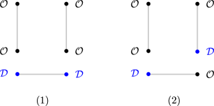
Figure A.4: Two diagrams for the two-loop ansatz.

These two diagrams correspond to two polynomials

$$P_{1}^{(2)}(x_{i})=x_{12}^{2}x_{34}^{2}x_{56}^{2}+S_{2}\times S_{4}\text{ permutations}\,,$$ (A.17)

$$P_{2}^{(2)}(x_{i})=x_{13}^{2}x_{24}^{2}x_{56}^{2}+S_{2}\times S_{4}\text{ permutations}\,,$$

where $S_{2}$ permutation permutes $x_{1},x_{2}$ and $S_{4}$ permutations permutes $x_{3},x_{4},x_{5},x_{6}$. Written down more explicitly, we have

$$P_{1}^{(2)}(x_{i})=16\,p_{1}(x_{i}),\qquad P_{2}^{(2)}(x_{i})=4\,p_{2}(x_{i})$$ (A.18)

where

$$p_{1}(x_{i})= \,x_{12}^{2}(x_{34}^{2}x_{56}^{2}+x_{35}^{2}x_{46}^{2}+x_{36}^{2}x_{45}^{2})\,,$$ (A.19)

$$p_{2}(x_{i})= \,x_{16}^{2}x_{25}^{2}x_{34}^{2}+x_{15}^{2}x_{26}^{2}x_{34}^{2}+x_{16}^{2}x_{24}^{2}x_{35}^{2}+x_{15}^{2}x_{24}^{2}x_{36}^{2}$$

$$\,+x_{14}^{2}x_{26}^{2}x_{35}^{2}+x_{14}^{2}x_{25}^{2}x_{36}^{2}+x_{16}^{2}x_{23}^{2}x_{45}^{2}+x_{15}^{2}x_{23}^{2}x_{46}^{2}$$

$$\,+x_{13}^{2}x_{26}^{2}x_{45}^{2}+x_{13}^{2}x_{25}^{2}x_{46}^{2}+x_{14}^{2}x_{23}^{2}x_{56}^{2}+x_{13}^{2}x_{24}^{2}x_{56}^{2}\,.$$

Therefore we make the ansatz

$$P^{(2)}=\frac{c_{1}P^{(2)}_{1}+c_{2}P_{2}^{(2)}}{(-4\pi^{2})^{2}}=\frac{c_{1}\,p_{1}+c_{2}\,p_{2}/4}{\pi^{4}}\,.$$ (A.20)

The ansatz has two unknown coefficients which we denote by $c_{1}$ and $c_{2}$. The corresponding two-loop integral can be written in terms of conformal 1- and 2-loop integrals as follows

$$\frac{G_{\{2,2\}}^{(2)}}{\tilde{R}_{1234}(d_{12})^{N-2}}= \,\left(c_{1}\,z\bar{z}+\frac{c_{2}}{4}(1-z)(1-\bar{z})+\frac{c_{2}}{4}\right)\left(F^{(1)}(z,\bar{z})\right)^{2}$$ (A.21)

$$\,+c_{2}\,F_{z}^{(2)}+2(c_{1}+c_{2}/4)F_{1-z}^{(2)}+c_{2}\,F^{(2)}_{\frac{z}{z-1}}\,,$$

where $F^{(1)}$ is the one-loop conformal integral. The various two-loop conformal integrals are defined by

$$F_{z}^{(2)}(z,\bar{z})=F^{(2)}(z,\bar{z}),\qquad F_{1-z}^{(2)}=F^{(2)}(1-z,1-\bar{z}),\qquad F^{(2)}_{\frac{z}{z-1}}=\frac{F^{(2)}\left(\frac{z}{z-1},\frac{\bar{z}}{\bar{z}-1}\right)}{(1-z)(1-\bar{z})}\,,$$ (A.22)

where $F^{(2)}$ is the two-loop conformal integral defined by

$$F^{(2)}(z,\bar{z})= \,\frac{x_{13}^{2}x_{24}^{2}x_{14}^{2}}{\pi^{4}}\int\frac{\mathrm{d}^{4}x_{5}\mathrm{d}^{4}x_{6}}{x_{15}^{2}x_{25}^{2}x_{45}^{2}x_{56}^{2}x_{16}^{2}x_{36}^{2}x_{46}^{2}}$$ (A.23)

$$= \,\frac{1}{z-\bar{z}}\left[\frac{\ln(z\bar{z})^{2}}{2}\left(\text{Li}_{2}(z)-\text{Li}_{2}(\bar{z})\right)-3\log(z\bar{z})\left(\text{Li}_{3}(z)-\text{Li}_{3}(\bar{z})\right)+6\left(\text{Li}_{4}(z)-\text{Li}_{4}(\bar{z})\right)\right]$$

$s$-channel OPE

In the $s$-channel, we have

$$\lim_{z,\bar{z}\to 0}F_{z}^{(2)}=\lim_{z,\bar{z}\to 0}F_{\frac{z}{z-1}}^{(2)}=\frac{1}{2}\ln^{2}u-3\ln u+6\,,\qquad\lim_{z,\bar{z}\to 0}F^{(2)}_{1-z}=6\zeta_{3}\,.$$ (A.24)

Using these results, the $s$-channel limit gives

$$\lim_{x_{1}\to x_{2}\atop x_{3}\to x_{4}}\frac{G_{\{2,2\}}^{(2)}}{\tilde{R}_{1234}(d_{12})^{N-2}}=\frac{3}{2}c_{2}(\ln u)^{2}-8c_{2}\,\ln u+12(c_{1}+c_{2}/4)\zeta(3)+14c_{2}\,.$$ (A.25)

On the other hand, we have

$$\left.\mathsf{d}_{\mathcal{K}}(g)\mathsf{c}_{\mathcal{K}}(g){u^{\delta\Delta/2}}\right|_{O(g^{4})}= \,\frac{1}{8}C_{0}\gamma_{1}^{2}\,(\ln u)^{2}+\frac{1}{2}(C_{1}\gamma_{1}+C_{0}\gamma_{2})(\ln u)+C_{2}$$ (A.26)

Using the results from the previous section and the known anomalous dimension of the Konishi operator, we have

$$C_{0}=\frac{1}{3},\qquad C_{1}=-4,\qquad\gamma_{1}=12,\qquad\gamma_{2}=-48\,.$$ (A.27)

Comparing (A.25) and (A.26), we find the equations

$$\frac{3}{2}c_{2}=\frac{1}{8}C_{0}\gamma_{1}^{2}=6,\qquad-8c_{2}=\frac{1}{2}(C_{1}\gamma_{1}+C_{0}\gamma_{2})$$ (A.28)

These are two equations for $c_{2}$. They are compatible and gives $c_{2}=4$. To determine the other unknown coefficient $c_{1}$, we consider the $t$-channel limit.

$t$-channel OPE

In the $t$-channel limit, we have

$$\lim_{z,\bar{z}\to 1}F_{z}^{(2)}=6\zeta_{3}\,,\qquad\lim_{z,\bar{z}\to 1}F^{(2)}_{1-z}=\lim_{z,\bar{z}\to 1}F^{(2)}_{\frac{z}{z-1}}=\frac{1}{2}(\ln v)^{2}-3\ln v+6$$ (A.29)

Using these results, in the $t$-channel limit, we obtain

$$\lim_{z,\bar{z}\to 1}\frac{G_{\{2,2\}}^{(2)}}{\tilde{R}_{1234}(d_{12})^{N-2}}=(2c_{1}+c_{2})(\ln v)^{2}-\left(10c_{1}+\frac{11c_{2}}{2}\right)\ln v+6c_{2}\zeta_{3}+(16c_{1}+10c_{2})\,.$$ (A.30)

From the OPE limit, we obtain

$$\lim_{z,\bar{z}\to 1}\frac{G_{\{2,2\}}^{(2)}}{\tilde{R}_{1234}(d_{12})^{N-2}}=\frac{1}{8}\widetilde{C}_{0}\tilde{\gamma}_{1}^{2}\,(\ln v)^{2}+\frac{1}{2}\left(\widetilde{C}_{1}\tilde{\gamma}_{1}+\widetilde{C}_{0}\tilde{\gamma}_{2}\right)\ln v+\widetilde{C}_{2}\,.$$ (A.31)

From the one-loop result, we find that

$$\widetilde{C}_{0}=1,\qquad\widetilde{C}_{1}=-4,\qquad\tilde{\gamma}_{1}=4\,.$$ (A.32)

Comparing the coefficients of $(\ln v)^{2}$, we find that

$$2c_{1}+c_{2}=\frac{1}{8}\widetilde{C}_{0}\tilde{\gamma}_{1}^{2}\quad\Longrightarrow\quad 2c_{1}+4=2$$ (A.33)

which leads to $c_{1}=-1$. Plugging $c_{1}=-1,c_{2}=4$ into (A.30), we find that

$$\tilde{\gamma}_{2}=-8,\qquad\widetilde{C}_{2}=24+24\zeta_{3}\,.$$ (A.34)

Plugging into (A.25), we further find that

$$C_{2}=56\,.$$ (A.35)

To sum up, up to two-loop order, we find that

$$P^{(2)}(x_{i})=\frac{p_{2}(x_{i})-p_{1}(x_{i})}{\pi^{4}}\,.$$ (A.36)

In the $s$-channel, we have

$$\gamma(g)=12g^{2}-48g^{4}+\ldots\,,\qquad\mathsf{d}_{\mathcal{K}}(g)\mathsf{c}_{\mathcal{K}}(g)=\frac{1}{3}-4g^{2}+56g^{4}+\ldots.$$ (A.37)

In the $t$-channel we have

$$\delta\Delta_{\text{open}}= \,4g^{2}-8g^{4}+\ldots,$$ (A.38)

$$\left(\mathsf{c}_{\text{Open}}(g)\right)^{2}= \,1-4g^{2}+24(1+\zeta_{3})g^{4}+\ldots$$

Appendix B Three-loop integrals

In this appendix, we list the three-loop integrals that are needed in the main text. These integrals were defined in […]

$$T(1,2;3,4)= \,\frac{x_{34}^{2}}{(-4\pi^{2})^{3}}\int\frac{\mathrm{d}^{4}x_{5}\mathrm{d}^{4}x_{6}\mathrm{d}^{4}x_{7}\,x_{17}^{2}}{(x_{15}^{2}x_{35}^{2})(x_{16}^{2}x_{46}^{2})(x_{37}^{2}x_{27}^{2}x_{47}^{2})x_{56}^{2}x_{57}^{2}x_{67}^{2}}\,,$$ (B.1)

$$E(1,2;3,4)= \,\frac{x_{23}^{2}x_{24}^{2}}{(-4\pi^{2})^{3}}\int\frac{\mathrm{d}^{4}x_{5}\mathrm{d}^{4}x_{6}\mathrm{d}^{4}x_{7}\,x_{16}^{2}}{(x_{15}^{2}x_{25}^{2}x_{35}^{2})x_{56}^{2}(x_{26}^{2}x_{36}^{2}x_{46}^{2})x_{67}^{2}(x_{17}^{2}x_{27}^{2}x_{47}^{2})}\,,$$

$$L(1,2;3,4)= \,\frac{x_{34}^{4}}{(-4\pi^{2})^{3}}\int\frac{\mathrm{d}^{4}x_{5}\mathrm{d}^{4}x_{6}\mathrm{d}^{4}x_{7}}{(x_{15}^{2}x_{35}^{2}x_{45}^{2})x_{56}^{2}(x_{36}^{2}x_{46}^{2})x_{67}^{2}(x_{27}^{2}x_{37}^{2}x_{47}^{2})}\,,$$

$$gh(1,2;3,4)= \,\frac{x_{12}^{2}x_{34}^{4}}{(-4\pi^{2})^{3}}\int\frac{\mathrm{d}^{4}x_{5}\mathrm{d}^{4}x_{6}\mathrm{d}^{4}x_{7}}{(x_{15}^{2}x_{25}^{2}x_{35}^{2}x_{45}^{2})(x_{16}^{2}x_{36}^{2}x_{46}^{2})(x_{27}^{2}x_{37}^{2}x_{47}^{2})x_{67}^{2}}\,,$$

$$H(1,2;3,4)= \,\frac{x_{14}^{2}x_{23}^{2}x_{34}^{2}}{(-4\pi^{2})^{3}}\int\frac{\mathrm{d}^{4}x_{5}\mathrm{d}^{4}x_{6}\mathrm{d}^{4}x_{7}\,x_{57}^{2}}{(x_{15}^{2}x_{25}^{2}x_{35}^{2}x_{45}^{2})x_{56}^{2}(x_{36}^{2}x_{46}^{2})x_{67}^{2}(x_{17}^{2}x_{27}^{2}x_{37}^{2}x_{47}^{2})}\,.$$

Notice that $gh(1,2;3,4)$ indeed factorizes into the product of two integrals, as the notation indicates

$$gh(1,2;3,4)=x_{12}^{2}x_{34}^{2}\,g(1,2,3,4)\times h(1,2;3,4)$$ (B.2)

where

$$g(1,2,3,4)= \,-\frac{1}{4\pi^{2}}\int\frac{\mathrm{d}^{4}x_{5}}{x_{15}^{2}x_{25}^{2}x_{35}^{2}x_{45}^{2}}\,,$$ (B.3)

$$h(1,2;3,4)= \,\frac{x_{34}^{2}}{(4\pi^{2})^{2}}\int\frac{\mathrm{d}^{4}x_{5}\mathrm{d}^{4}x_{6}}{(x_{15}^{2}x_{35}^{2}x_{45}^{2})x_{56}^{2}(x_{26}^{2}x_{36}^{2}x_{46}^{2})}\,.$$

B.1 Symmetry of integrals

The integrals defined in (B.1) satisfy certain relations under re-ordering the labels. We list them here.

Manifest invariance

These are the symmetries that are already manifest at the level of integrands.

$$L(1,2;3,4)=L(2,1;3,4),\quad L(1,2;4,3)=L(1,2;3,4)\,,$$ (B.4)

$$H(1,2;3,4)=H(2,1;4,3),\quad E(1,2;4,3)=E(1,2;3,4)\,.$$

Flip identities

$$L(1,2;3,4)=L(3,4;1,2),\quad E(1,2;3,4)=E(3,4;1,2),$$ (B.5)

$$H(1,2;3,4)=H(3,4;1,2),\quad E(1,2;3,4)=E(2,1;3,4)\,.$$

Identity between integrals

Finally we have

$$T(1,2;3,4)=L(1,2;3,4)\,.$$ (B.6)

Additional relations

There are some additional relations which are also useful in the main text.

$$H(1,2;4,3)=\frac{1}{v}H(1,2;3,4)$$ (B.7)

B.2 $s$-channel asymptotics

In the main text, we need to use the value of the integrals in the $s$-channel OPE limit $x_{1}\to x_{2}$, $x_{3}\to x_{4}$, which is equivalent to $u\to 0$, $v\to 1$ in terms of conformal cross ratios. The leading order contribution in this limit has been worked out for the various integrals, which we list here. We first have

$$x_{24}^{4}\,g(1,2,3,4)_{s}= \,\frac{1}{4}\ln u-\frac{1}{2}\,,$$ (B.8)

$$x_{24}^{4}\,h(1,2;3,4)_{s}= \,\frac{3}{8}\zeta(3)\,,$$

$$x_{24}^{4}\,h(1,3;2,4)_{s}= \,\frac{1}{32}(\ln u)^{2}-\frac{3}{16}\ln u+\frac{3}{8}\,,$$

$$x_{24}^{4}\,h(1,4;2,3)_{s}= \,\frac{1}{32}(\ln u)^{2}-\frac{3}{16}\ln u+\frac{3}{8}\,.$$

which leads to

$$x_{24}^{4}\,gh(1,2;3,4)_{s}= \,\frac{3}{32}\zeta(3)\,\ln u-\frac{3}{16}\zeta(3)\,,$$ (B.9)

$$x_{24}^{4}\,gh(1,3;2,4)_{s}= \,\frac{1}{128}(\ln u)^{3}-\frac{1}{16}(\ln u)^{2}+\frac{3}{16}\ln u-\frac{3}{16}\,,$$

$$x_{24}^{4}\,gh(1,4;2,3)_{s}= \,\frac{1}{128}(\ln u)^{3}-\frac{1}{16}(\ln u)^{2}+\frac{3}{16}\ln u-\frac{3}{16}\,.$$

The rest of the asymptotic integrals are given by

$$x_{24}^{4}\,L(1,2;3,4)_{s}= \,-\frac{5}{16}\zeta(5)\,,$$ (B.10)

$$x_{24}^{4}\,L(1,3;2,4)_{s}= \,\frac{1}{384}(\ln u)^{3}-\frac{1}{32}(\ln u)^{2}+\frac{5}{32}\ln u-\frac{5}{16}\,,$$

$$x_{24}^{4}\,L(1,4;2,3)_{s}= \,\frac{1}{384}(\ln u)^{3}-\frac{1}{32}(\ln u)^{2}+\frac{5}{32}\ln u-\frac{5}{16}\,.$$

$$x_{24}^{4}\,E(1,2;3,4)_{s}= \,\frac{1}{192}(\ln u)^{3}-\frac{3}{64}(\ln u)^{2}+\frac{5}{32}\ln u-\frac{5}{16}\zeta(5)+\frac{3}{32}\zeta(3)-\frac{5}{32}\,,$$ (B.11)

$$x_{24}^{4}\,E(1,3;2,4)_{s}= \,\frac{3}{32}\zeta(3)\,\ln u-\frac{3}{16}\zeta(3)\,,$$

$$x_{24}^{4}\,E(1,4;2,3)_{s}= \,\frac{3}{32}\zeta(3)\,\ln u-\frac{3}{16}\zeta(3)\,.$$

$$x_{24}^{4}\,H(1,2;3,4)_{s}= \,\frac{3}{16}\zeta(3)\,\ln u-\frac{3}{16}\zeta(3)\,,$$ (B.12)

$$x_{24}^{4}\,H(1,3;2,4)_{s}= \,\frac{1}{192}(\ln u)^{3}-\frac{1}{16}(\ln u)^{2}+\frac{9}{32}\ln u+\frac{1}{4}\zeta(3)-\frac{7}{16}\,,$$

$$x_{24}^{4}\,H(1,4;2,3)_{s}= \,\frac{1}{192}(\ln u)^{3}-\frac{1}{16}(\ln u)^{2}+\frac{9}{32}\ln u+\frac{1}{4}\zeta(3)-\frac{7}{16}\,,$$

where we use an index ‘$s$’ to denote the $s$-channel OPE limit. The asymptotic results above can be examined by numerical calculation via AMFlow and Fiesta Liu:2022chg ; Smirnov:2021rhf .

B.3 $t$-channel asymptotics

The asymptotic behavior of the three-loop integral in $t$-channel can be obtained by the following trick. The $t$-channel limit $x_{1}\to x_{4}$, $x_{2}\to x_{3}$ can be obtained by: (1) Swap $x_{2}$ and $x_{4}$; (2) Take the $s$-channel OPE limit in the new configuration. Notice that when swapping $x_{2}$ and $x_{4}$, we also swap the role of $u$ and $v$. Since all integrals involved are single-valued harmonic polylogarithms, this trick allows us to make use of the $s$-channel OPE which was derived in the previous subsection. For example, the $t$-channel asymptotic behavior of $H(1,2;3,4)$ can be obtained as

$$H(1,2;3,4)_{t}\overset{x_{2}\leftrightarrow x_{4}}{=}\left.H(1,4;3,2)_{s}\right|_{u\to v}=\left.uH(1,4;2,3)_{s}\right|_{u\to v}\,.$$ (B.13)

Therefore, the asymptotic behavior of $H(1,2;3,4)$ in the $t$-channel is

$$x_{24}^{4}\,H(1,2;3,4)_{t}=v\left(\frac{1}{192}\ln(v)^{3}-\frac{1}{16}\ln(v)^{2}+\frac{9}{32}\ln(v)+\frac{1}{4}\zeta(3)\right).$$ (B.14)

Using this trick, we obtain the $t$-channel asymptotics of the three-loop integrals, which is listed as follows

$$x_{24}^{4}\,gh(1,4;2,3)_{t}= \,-\frac{3v}{16}\zeta(3)+\frac{3v}{32}\zeta(3)\ln v\,,$$ (B.15)

$$x_{24}^{4}\,gh(1,2;3,4)_{t}= \,\frac{1}{128}(\ln v)^{3}-\frac{1}{16}(\ln v)^{2}+\frac{3}{16}\ln v-\frac{3}{16}\,,$$

$$x_{24}^{4}\,gh(1,3;2,4)_{t}= \,\frac{1}{128}(\ln v)^{3}-\frac{1}{16}(\ln v)^{2}+\frac{3}{16}\ln v-\frac{3}{16}\,.$$

$$x_{24}^{4}\,L(1,4;2,3)_{t}= \,-\frac{5}{16}\zeta(5)\,,$$ (B.16)

$$x_{24}^{4}\,L(1,3;2,4)_{t}= \,\frac{1}{384}(\ln v)^{3}-\frac{1}{32}(\ln v)^{2}+\frac{5}{32}\ln v-\frac{5}{16}\,,$$

$$x_{24}^{4}\,L(1,2;3,4)_{t}= \,\frac{1}{384}(\ln v)^{3}-\frac{1}{32}(\ln v)^{2}+\frac{5}{32}\ln v-\frac{5}{16}.$$

$$x_{24}^{4}\,E(1,4;2,3)_{t}= \,\frac{1}{192}(\ln v)^{3}-\frac{3}{64}(\ln v)^{2}+\frac{5}{32}\ln v-\frac{5}{16}\zeta(5)+\frac{3}{32}\zeta(3)-\frac{5}{32}$$ (B.17)

$$x_{24}^{4}\,E(1,2;3,4)_{t}= \,\frac{3}{32}\zeta(3)\ln v-\frac{3}{16}\zeta(3)\,,$$

$$x_{24}^{4}\,E(1,3;2,4)_{t}= \,\frac{3}{32}\zeta(3)\ln v-\frac{3}{16}\zeta(3)\,,$$

$$x_{24}^{4}\,H(1,4;2,3)_{t}= \,\frac{3}{16}\zeta(3)\ln v-\frac{3}{16}\zeta(3)\,,$$ (B.18)

$$x_{24}^{4}\,H(1,2;3,4)_{t}= \,\frac{v}{192}(\ln v)^{3}-\frac{v}{16}(\ln v)^{2}+\frac{9v}{32}\ln v+\frac{v}{4}\zeta(3)-\frac{7v}{16}\,,$$

$$x_{24}^{4}\,H(1,3;2,4)_{t}= \,\frac{v}{192}(\ln v)^{3}-\frac{v}{16}(\ln v)^{2}+\frac{9v}{32}\ln v+\frac{v}{4}\zeta(3)-\frac{7v}{16}\,,$$

Appendix C Large spin limit

The asymptotic behavior of harmonic sums can be computed by the method in Ablinger:2012ufz . The main idea of this method is to use the relation between harmonic sums and Mellin transformation of harmonic polylogarithms. Mellin transformation is defined as

$$\mathrm{M}(f(x),n)=\int^{1}_{0}x^{n}f(x).$$ (C.1)

Harmonic polylogarithms under this transformation have the following propertiesAblinger:2012ufz :

$$\mathrm{M}\left(\frac{\mathrm{H}_{\bm{m}}(x)}{1-x},n+1\right)=-(n+1)\mathrm{M}(\mathrm{H}_{1,\bm{m}}(x),n),$$ (C.2)

$$\mathrm{M}\left(\frac{\mathrm{H}_{\textbf{m}}(x)}{1+x},n+1\right)=-(n+1)\mathrm{M}(\mathrm{H}_{-1,\bm{m}}(x),n)+\mathrm{H}_{-1,\bm{m}}(1),$$ (C.3)

$$\mathrm{M}\left(\mathrm{H}_{0}(x),n\right) =-\frac{1}{(n+1)^{2}}$$ (C.4)

$$\mathrm{M}\left(\mathrm{H}_{1}(x),n\right) =\frac{\mathrm{S}_{1}(n+1)}{n+1}$$

$$\mathrm{M}\left(\mathrm{H}_{-1}(x),n\right) =(-1)^{n}\frac{\mathrm{S}_{-1}(n+1)}{n+1}+\frac{\mathrm{H}_{-1}(1)}{n+1}\left(1+(-1)^{n}\right)$$

$$\mathrm{M}\left(\mathrm{H}_{0,\bm{m}}(x),n\right) =\frac{\mathrm{H}_{0,\bm{m}}(1)}{n+1}-\frac{1}{n+1}\mathrm{M}\left(\mathrm{H}_{\bm{m}}(x),n\right)$$ (C.5)

$$\mathrm{M}\left(\mathrm{H}_{1,\bm{m}}(x),n\right) =\frac{1}{n+1}\sum_{i=0}^{n}\mathrm{M}\left(\mathrm{H}_{m}(x),n\right)$$

$$\mathrm{M}\left(\mathrm{H}_{-1,\bm{m}}(x),n\right) =\frac{1+(-1)^{n}}{n+1}\mathrm{H}_{-1,\bm{m}}(1)-\frac{(-1)^{n}}{n+1}\sum_{i=0}^{n}(-1)^{i}\mathrm{M}\left(\mathrm{H}_{m}(x),n\right).$$

According to these properties, $\mathrm{M}(\mathrm{H}_{\bm{m}}(x),n)$, $\mathrm{M}(\frac{\mathrm{H}_{\bm{m}}(x)}{1-x},n)$ and $\mathrm{M}(\frac{\mathrm{H}_{\bm{m}}(x)}{1+x},n)$ can be recursively calculated and expressed in terms of the harmonic sums with the argument $n$, the harmonic sums at infinity and harmonic polylogarithms at one. Inversely, for specific harmonic sum $\mathrm{S}_{\bm{a}}(n)$, we can find $\frac{\mathrm{H}_{\bm{m}}(x)}{1+\omega x}$ such that $\mathrm{S}_{\bm{a}}(n)$ is the most complicated term in $\mathrm{M}(\frac{\mathrm{H}_{\bm{m}}(x)}{1+\omega x},n)$, i.e.,

$$\mathrm{S}_{\bm{a}}(n)=\mathrm{M}\left(\frac{\mathrm{H}_{\bm{m}}(x)}{1+\omega x},n\right)+\mathrm{T},$$ (C.6)

where $\mathrm{T}$ is an expression in less complicated harmonic sums and constants. The detailed procedure is given by $Algoritm\ 2$ in Ablinger:2009ovq . According to the relation above, the asymptotic behavior of $\mathrm{S}_{\bm{a}}(n)$ can be computed by the asymptotic expansion of $\mathrm{M}(\frac{\mathrm{H}_{\bm{m}}(x)}{1+\omega x},n)$. Here is an example:

$$\mathrm{S}_{3,1}(n)=-\mathrm{M}\left(\frac{\mathrm{H}_{0,0,1}(x)}{1-x},n\right)-\mathrm{S}_{1}(n)\mathrm{S}_{3}(\infty)+\mathrm{S}_{2}(n)\mathrm{S}_{2}(\infty),$$ (C.7)

$$\mathrm{M}\left(\frac{\mathrm{H}_{0,0,1}(x)}{1-x},n\right)=\frac{\mathrm{S}_{2}(\infty)^{2}}{2}-\mathrm{S}_{3}(\infty)\mathrm{S}_{1}(n)-\frac{S_{2}(\infty)}{n}+\mathcal{O}(\frac{1}{n^{2}}).$$ (C.8)

Thus,

$$\mathrm{S}_{3,1}(n)=\frac{\mathrm{S}_{2}(\infty)^{2}}{2}+\mathcal{O}(\frac{1}{n^{2}}).$$ (C.9)

Here we replace the value of harmonic polylogarithms at one with the value of harmonic sums at infinity, and reduce the constant value through relations between harmonic sums at infinity. These relations contain quasi shuffle relations and the following relationVermaseren:1998uu :

$$\mathrm{S}_{m_{1},\ldots,m_{p}}(\infty)\mathrm{S}_{k_{1},\ldots,k_{q}}(\infty)=\lim_{n\rightarrow\infty}\sum_{i=1}^{n}\frac{\operatorname{sign}\left(k_{1}\right)^{i}\mathrm{~{}S}_{m_{1},\ldots,m_{p}}(n-i)\mathrm{S}_{k_{2},\ldots,k_{q}}(i)}{i^{\left|k_{1}\right|}}.$$ (C.10)

Considering these relations, the value of harmonic sum at infinity can be reduced to basis constants.

Some constant values of harmonic sums at infinity can be found in Alday:2013cwa .

References

- (1) D. Poland, S. Rychkov and A. Vichi, The Conformal Bootstrap: Theory, Numerical Techniques, and Applications, Rev. Mod. Phys. 91 (2019) 015002 [1805.04405].
- (2) D. Poland and D. Simmons-Duffin, Snowmass White Paper: The Numerical Conformal Bootstrap, in Snowmass 2021, 3, 2022 [2203.08117].
- (3) T. Hartman, D. Mazac, D. Simmons-Duffin and A. Zhiboedov, Snowmass White Paper: The Analytic Conformal Bootstrap, in Snowmass 2021, 2, 2022 [2202.11012].
- (4) S. Caron-Huot, F. Coronado, A.-K. Trinh and Z. Zahraee, Bootstrapping = 4 sYM correlators using integrability, JHEP 02 (2023) 083 [2207.01615].
- (5) A. Cavaglià, N. Gromov, J. Julius and M. Preti, Integrability and conformal bootstrap: One dimensional defect conformal field theory, Phys. Rev. D 105 (2022) L021902 [2107.08510].
- (6) A. Cavaglià, N. Gromov, J. Julius and M. Preti, Bootstrability in defect CFT: integrated correlators and sharper bounds, JHEP 05 (2022) 164 [2203.09556].
- (7) B. Eden, P. Heslop, G.P. Korchemsky and E. Sokatchev, Hidden symmetry of four-point correlation functions and amplitudes in N=4 SYM, Nucl. Phys. B 862 (2012) 193 [1108.3557].
- (8) B. Eden, P. Heslop, G.P. Korchemsky and E. Sokatchev, Constructing the correlation function of four stress-tensor multiplets and the four-particle amplitude in N=4 SYM, Nucl. Phys. B 862 (2012) 450 [1201.5329].
- (9) D. Chicherin, J. Drummond, P. Heslop and E. Sokatchev, All three-loop four-point correlators of half-BPS operators in planar = 4 SYM, JHEP 08 (2016) 053 [1512.02926].
- (10) D. Chicherin, A. Georgoudis, V. Gonçalves and R. Pereira, All five-loop planar four-point functions of half-BPS operators in SYM, JHEP 11 (2018) 069 [1809.00551].
- (11) J.L. Bourjaily, P. Heslop and V.-V. Tran, Amplitudes and Correlators to Ten Loops Using Simple, Graphical Bootstraps, JHEP 11 (2016) 125 [1609.00007].
- (12) E. D’Hoker, D.Z. Freedman, S.D. Mathur, A. Matusis and L. Rastelli, Graviton exchange and complete four point functions in the AdS / CFT correspondence, Nucl. Phys. B 562 (1999) 353 [hep-th/9903196].
- (13) G. Arutyunov and S. Frolov, Four point functions of lowest weight CPOs in N=4 SYM(4) in supergravity approximation, Phys. Rev. D 62 (2000) 064016 [hep-th/0002170].
- (14) L. Rastelli and X. Zhou, Mellin amplitudes for , Phys. Rev. Lett. 118 (2017) 091602 [1608.06624].
- (15) L. Rastelli and X. Zhou, How to Succeed at Holographic Correlators Without Really Trying, JHEP 04 (2018) 014 [1710.05923].
- (16) L.F. Alday and X. Zhou, Simplicity of AdS Supergravity at One Loop, JHEP 09 (2020) 008 [1912.02663].
- (17) L.F. Alday and X. Zhou, All Holographic Four-Point Functions in All Maximally Supersymmetric CFTs, Phys. Rev. X 11 (2021) 011056 [2006.12505].
- (18) J.M. Drummond and H. Paul, One-loop string corrections to AdS amplitudes from CFT, JHEP 03 (2021) 038 [1912.07632].
- (19) F. Aprile, J. Drummond, P. Heslop and H. Paul, One-loop amplitudes in AdS supergravity from = 4 SYM at strong coupling, JHEP 03 (2020) 190 [1912.01047].
- (20) J.M. Drummond and H. Paul, Two-loop supergravity on AdS from CFT, JHEP 08 (2022) 275 [2204.01829].
- (21) S. Caron-Huot and A.-K. Trinh, All tree-level correlators in AdS supergravity: hidden ten-dimensional conformal symmetry, JHEP 01 (2019) 196 [1809.09173].
- (22) S. Caron-Huot and F. Coronado, Ten dimensional symmetry of = 4 SYM correlators, JHEP 03 (2022) 151 [2106.03892].
- (23) L.F. Alday, T. Hansen and J.A. Silva, AdS Virasoro-Shapiro from dispersive sum rules, JHEP 10 (2022) 036 [2204.07542].
- (24) L.F. Alday, T. Hansen and J.A. Silva, AdS Virasoro-Shapiro from single-valued periods, JHEP 12 (2022) 010 [2209.06223].
- (25) L.F. Alday, T. Hansen and J.A. Silva, On the spectrum and structure constants of short operators in N=4 SYM at strong coupling, JHEP 08 (2023) 214 [2303.08834].
- (26) L.F. Alday, T. Hansen and J.A. Silva, Emergent Worldsheet for the AdS Virasoro-Shapiro Amplitude, Phys. Rev. Lett. 131 (2023) 161603 [2305.03593].
- (27) L.F. Alday and T. Hansen, The AdS Virasoro-Shapiro amplitude, JHEP 10 (2023) 023 [2306.12786].
- (28) G. Fardelli, T. Hansen and J.A. Silva, AdS Virasoro-Shapiro amplitude with KK modes, JHEP 11 (2023) 064 [2308.03683].
- (29) T. Fleury and S. Komatsu, Hexagonalization of Correlation Functions, JHEP 01 (2017) 130 [1611.05577].
- (30) T. Fleury and S. Komatsu, Hexagonalization of Correlation Functions II: Two-Particle Contributions, JHEP 02 (2018) 177 [1711.05327].
- (31) B. Basso, F. Coronado, S. Komatsu, H.T. Lam, P. Vieira and D.-l. Zhong, Asymptotic Four Point Functions, JHEP 07 (2019) 082 [1701.04462].
- (32) F. Coronado, Perturbative four-point functions in planar SYM from hexagonalization, JHEP 01 (2019) 056 [1811.00467].
- (33) F. Coronado, Bootstrapping the Simplest Correlator in Planar Supersymmetric Yang-Mills Theory to All Loops, Phys. Rev. Lett. 124 (2020) 171601 [1811.03282].
- (34) T. Bargheer, J. Caetano, T. Fleury, S. Komatsu and P. Vieira, Handling Handles: Nonplanar Integrability in Supersymmetric Yang-Mills Theory, Phys. Rev. Lett. 121 (2018) 231602 [1711.05326].
- (35) T. Bargheer, J. Caetano, T. Fleury, S. Komatsu and P. Vieira, Handling handles. Part II. Stratification and data analysis, JHEP 11 (2018) 095 [1809.09145].
- (36) T. Fleury and R. Pereira, Non-planar data of = 4 SYM, JHEP 03 (2020) 003 [1910.09428].
- (37) T. Bargheer, F. Coronado and P. Vieira, Octagons I: Combinatorics and Non-Planar Resummations, JHEP 08 (2019) 162 [1904.00965].
- (38) J. McGreevy, L. Susskind and N. Toumbas, Invasion of the giant gravitons from Anti-de Sitter space, JHEP 06 (2000) 008 [hep-th/0003075].
- (39) V. Balasubramanian, M. Berkooz, A. Naqvi and M.J. Strassler, Giant gravitons in conformal field theory, JHEP 04 (2002) 034 [hep-th/0107119].
- (40) A. Hashimoto, S. Hirano and N. Itzhaki, Large branes in AdS and their field theory dual, JHEP 08 (2000) 051 [hep-th/0008016].
- (41) S. Corley, A. Jevicki and S. Ramgoolam, Exact correlators of giant gravitons from dual N=4 SYM theory, Adv. Theor. Math. Phys. 5 (2002) 809 [hep-th/0111222].
- (42) R. de Mello Koch and R. Gwyn, Giant graviton correlators from dual SU(N) super Yang-Mills theory, JHEP 11 (2004) 081 [hep-th/0410236].
- (43) Y. Kimura and S. Ramgoolam, Branes, anti-branes and brauer algebras in gauge-gravity duality, JHEP 11 (2007) 078 [0709.2158].
- (44) A. Bissi, C. Kristjansen, D. Young and K. Zoubos, Holographic three-point functions of giant gravitons, JHEP 06 (2011) 085 [1103.4079].
- (45) P. Caputa, R. de Mello Koch and K. Zoubos, Extremal versus Non-Extremal Correlators with Giant Gravitons, JHEP 08 (2012) 143 [1204.4172].
- (46) D. Berenstein, Giant gravitons: a collective coordinate approach, Phys. Rev. D 87 (2013) 126009 [1301.3519].
- (47) Y. Kimura, S. Ramgoolam and R. Suzuki, Flavour singlets in gauge theory as Permutations, JHEP 12 (2016) 142 [1608.03188].
- (48) R. de Mello Koch, E. Gandote and J.-H. Huang, Non-Perturbative String Theory from AdS/CFT, JHEP 02 (2019) 169 [1901.02591].
- (49) G. Chen, R. de Mello Koch, M. Kim and H.J.R. Van Zyl, Absorption of closed strings by giant gravitons, JHEP 10 (2019) 133 [1908.03553].
- (50) G. Chen, R. De Mello Koch, M. Kim and H.J.R. Van Zyl, Structure constants of heavy operators in ABJM and ABJ theory, Phys. Rev. D 100 (2019) 086019 [1909.03215].
- (51) Y. Jiang, S. Komatsu and E. Vescovi, Structure constants in = 4 SYM at finite coupling as worldsheet g-function, JHEP 07 (2020) 037 [1906.07733].
- (52) Y. Jiang, S. Komatsu and E. Vescovi, Exact Three-Point Functions of Determinant Operators in Planar Supersymmetric Yang-Mills Theory, Phys. Rev. Lett. 123 (2019) 191601 [1907.11242].
- (53) P. Yang, Y. Jiang, S. Komatsu and J.-B. Wu, Three-point functions in ABJM and Bethe Ansatz, JHEP 01 (2022) 002 [2103.15840].
- (54) P. Yang, Y. Jiang, S. Komatsu and J.-B. Wu, D-branes and orbit average, SciPost Phys. 12 (2022) 055 [2103.16580].
- (55) E. Vescovi, Four-point function of determinant operators in SYM, Phys. Rev. D 103 (2021) 106001 [2101.05117].
- (56) H. Lin, Coherent state excitations and string-added coherent states in gauge-gravity correspondence, Nucl. Phys. B 986 (2023) 116066 [2206.06524].
- (57) H. Lin, Coherent state operators, giant gravitons, and gauge-gravity correspondence, Annals Phys. 451 (2023) 169248 [2212.14002].
- (58) L.F. Alday, B. Eden, G.P. Korchemsky, J. Maldacena and E. Sokatchev, From correlation functions to Wilson loops, JHEP 09 (2011) 123 [1007.3243].
- (59) B. Eden, P. Heslop, G.P. Korchemsky and E. Sokatchev, The super-correlator/super-amplitude duality: Part I, Nucl. Phys. B 869 (2013) 329 [1103.3714].
- (60) B. Eden, A.C. Petkou, C. Schubert and E. Sokatchev, Partial nonrenormalization of the stress tensor four point function in N=4 SYM and AdS / CFT, Nucl. Phys. B 607 (2001) 191 [hep-th/0009106].
- (61) M. Nirschl and H. Osborn, Superconformal Ward identities and their solution, Nucl. Phys. B 711 (2005) 409 [hep-th/0407060].
- (62) B. Eden, G.P. Korchemsky and E. Sokatchev, From correlation functions to scattering amplitudes, JHEP 12 (2011) 002 [1007.3246].
- (63) N. Gromov, V. Kazakov, S. Leurent and D. Volin, Quantum Spectral Curve for Planar Super-Yang-Mills Theory, Phys. Rev. Lett. 112 (2014) 011602 [1305.1939].
- (64) C. Marboe, V. Velizhanin and D. Volin, Six-loop anomalous dimension of twist-two operators in planar SYM theory, JHEP 07 (2015) 084 [1412.4762].
- (65) B. Basso, S. Komatsu and P. Vieira, Structure Constants and Integrable Bootstrap in Planar N=4 SYM Theory, 1505.06745.
- (66) B. Basso, A. Georgoudis and A.K. Sueiro, Structure Constants of Short Operators in Planar N=4 Supersymmetric Yang-Mills Theory, Phys. Rev. Lett. 130 (2023) 131603 [2207.01315].
- (67) A. Georgoudis, V. Goncalves and R. Pereira, Konishi OPE coefficient at the five loop order, JHEP 11 (2018) 184 [1710.06419].
- (68) J.M. Drummond, J. Henn, V.A. Smirnov and E. Sokatchev, Magic identities for conformal four-point integrals, JHEP 01 (2007) 064 [hep-th/0607160].
- (69) C. Anastasiou, Z. Bern, L.J. Dixon and D.A. Kosower, Planar amplitudes in maximally supersymmetric Yang-Mills theory, Phys. Rev. Lett. 91 (2003) 251602 [hep-th/0309040].
- (70) P. Vieira and T. Wang, Tailoring Non-Compact Spin Chains, JHEP 10 (2014) 035 [1311.6404].
- (71) J. Ablinger, The package HarmonicSums: Computer Algebra and Analytic aspects of Nested Sums, PoS LL2014 (2014) 019 [1407.6180].
- (72) B. Basso, V. Goncalves, S. Komatsu and P. Vieira, Gluing Hexagons at Three Loops, Nucl. Phys. B 907 (2016) 695 [1510.01683].
- (73) Y. Jiang, S. Komatsu, I. Kostov and D. Serban, Clustering and the Three-Point Function, J. Phys. A 49 (2016) 454003 [1604.03575].
- (74) I. Kostov, V.B. Petkova and D. Serban, Determinant Formula for the Octagon Form Factor in =4 Supersymmetric Yang-Mills Theory, Phys. Rev. Lett. 122 (2019) 231601 [1903.05038].
- (75) A.V. Belitsky and G.P. Korchemsky, Octagon at finite coupling, JHEP 07 (2020) 219 [2003.01121].
- (76) T. Bargheer, F. Coronado and P. Vieira, Octagons II: Strong Coupling, 1909.04077.
- (77) X. Liu and Y.-Q. Ma, AMFlow: A Mathematica package for Feynman integrals computation via auxiliary mass flow, Comput. Phys. Commun. 283 (2023) 108565 [2201.11669].
- (78) A.V. Smirnov, N.D. Shapurov and L.I. Vysotsky, FIESTA5: Numerical high-performance Feynman integral evaluation, Comput. Phys. Commun. 277 (2022) 108386 [2110.11660].
- (79) J. Ablinger, Computer Algebra Algorithms for Special Functions in Particle Physics, Ph.D. thesis, Linz U., 4, 2012. 1305.0687.
- (80) J. Ablinger, A Computer Algebra Toolbox for Harmonic Sums Related to Particle Physics, Master’s thesis, Linz U., 2009, [1011.1176].
- (81) J.A.M. Vermaseren, Harmonic sums, Mellin transforms and integrals, Int. J. Mod. Phys. A 14 (1999) 2037 [hep-ph/9806280].
- (82) L.F. Alday and A. Bissi, Higher-spin correlators, JHEP 10 (2013) 202 [1305.4604].