Singular electromagnetic fields in nonlinear electrodynamics with a constant background field

Abstract

When exploring equations of nonlinear electrodynamics in effective medium formed by mutually parallel external electric and magnetic fields, we come to special static axial-symmetric solutions of two types. The first are comprised of fields referred to as electric and magnetic responses to a point-like electric charge when placed into the medium. In electric case, this is a field determined by the induced charge density. In magnetic case, this is a field carrying no magnetic charge and determined by an induced current. Fields of second type require presence of pseudoscalar constants for their existence. These are singular on the axis drawn along the external fields. In electric case this is a field of an inhomogeneously charged infinitely thin thread. In magnetic case this is the magnetic monopole with the Dirac string supported by solenoidal current. In both cases the necessary pseudoscalar constant is supplied by field derivatives of nonlinear Lagrangian taken on external fields. There is also a magnetic thread solution dual to electric thread with null total magnetic charge.

1 Introduction

The search for nonlinear effects stimulated by fields is a subject of widespread interest across diverse areas of physics. In Quantum Electrodynamics (QED), for instance, the nonlinearity supplied by strong electromagnetic fields – which has been known ever since the seminal works by Klein [1], Sauter [2], Heisenberg and Euler [3], Weiskpoff [4], Euler and Köckel [5], and Schwinger [6] – is attracting considerable attention lately owing to advances in laser technology, driven especially by chirped pulse amplification [7]. Thanks to this, there is a growing number of ongoing and planned experiments devoted to detecting nonlinear quantum phenomena stemming from ultra-intense focused laser pulse collisions. The subject is well discussed in a number of reviews [8, 9, 10, 11, 12, 13, 14, 15, 16] and references therein (see also the references [17, 18, 19, 20, 21, 22, 23, 24] for theoretical foundations of QED with external fields).

From a fundamental perspective, the nonlinearity in QED is provided  by the scattering of light by light, which is described by the four-photon diagram. Its experimental observation in collisions of nuclei was recently reported in [25]. On the other hand, it is long since understood that nonlinear process of photon splitting into two [26], [27] shows itself in formation of radiation [28] produced by highly magnetized neutron stars (pulsars). Owing to the nonlinearity, the vacuum filled with strong electromagnetic fields makes an equivalent medium described by polarization and mass operators calculated through Feynman diagrams with “dressed” propagators for electrons and positrons, i.e., in the Furry representation [29], with exact solutions of the Dirac equation in external-field background for them. The common primary goal for observation [30] of nonlinearity of QED is the birefringence of vacuum [26], [31], [32] filled with a strong field (notably, the recent evidence for it is obtained from a neutron star [33])).

While the rigorous treatment of nonlinear quantum effects in QED requires the knowledge of polarization tensors calculated within the Furry representation, essential simplification can be achieved by computing them with the aid of effective Lagrangians in the local approximation, depending exclusively on field strengths (and not their space-time derivatives). This approximation, which supplements Maxwell’s electrodynamics with effective actions, provides an excellent framework for investigating phenomenological consequences of the nonlinear character of the vacuum with external fields.

Models based on nonlinear electrodynamics are gaining considerable attention in diverse areas, such as in Einstein’s General Relativity (GR) coupled to electromagnetic fields. In this instance, the influence on the Universe’s evolution is under study, and a variety of new types of charged black holes appear, among which the magnetized black holes are closest to the authors’ interests; see, e.g., [34] and references therein. In the context of particle physics, there is an intense activity regarding the experimental search for magnetic monopoles basing on experiments on high-energy peripheral nucleus-nucleus collisions, wherein pure photon-photon interaction is distinguishable, whose consideration resulted in discovery of the long-waited-for light-by-light scattering [36]. The same photon-photon interaction may become responsible for monopole-antimonopole pairs production. Among nonlinear models recruited to treat the photon-photon interaction, Born-Infeld extensions of the Standard Model attract special attention (see e.g. [37, 38, 39]), as following from string theory [40] and providing finiteness of the field energy to a point-like monopole, both electric or magnetic, identified with its mass. See also Refs. [43, 44, 45] for alternative models and Refs. [46, 47, 48, 49] for experimental searches within MoEDAL’s collaboration [50, 51, 52]. There is also the possibility of monopole-antimonopole pair creation from the vacuum by strong magnetic fields produced during colorredthe mentioned peripheral collisions. [53, 54, 55, 56, 57]. Besides these subjects, models based on nonlinear electrodynamics were also considered in radiation problems e.g. [58], systems coupled to axion fields/dark-matter models e.g. [59, 60, 61, 62], and even in condensed matter physics [63].

In the present paper, we study nonlinear Maxwell’s equations for electromagnetic fields produced by a point charge placed in strong electromagnetic fields. We are basing on the general local nonlinear electrodynamics, whose action is an arbitrary nonlinear functional of electric and magnetic field strengths independent of their time- and space-derivatives. Examples of such theories are provided by the so-called Heisenberg-Euler action calculated within one-loop [3] and two-loop [67] accuracy in QED, by the famous Born-Infeld [68] action and by many other models considered together with GR, see references in [34]. All results are expressed in terms of derivatives over fields of the general nonlinear local Lagrangian.

In Sec. 2 perturbation expansion to solutions of nonlinear Maxwell equations with respect of small nonlinearity is outlined, and the electric charge and current density induced by the point-like electric charge are obtained against the external-field background. We find, first, the electric response to that charge, which reduces to its screening and to inducing an angle-distributed electric charge density. Next, we find an angle-depending magnetic response due to the induced current. It carries no magnetic charge and it is depicted in Fig. 1 (see also [69], [70]). In Sec. 3, we supplement the responses of Sec. 2 with arbitrary-magnitude solutions of corresponding homogeneous equations. These combined fields suffer singularities on lines parallel to the common direction of the background fields. The electric contribution to the combined field is found in Subsection3.1. It requires to be supported by a charge concentrated on an infinitely thin thread, and an outer pseudoscalar constant formed by the background fields is needed. The magnetic contribution to the combined field is found in Subsection3.2 This is a magnetic monopole rigged with the field contained in an infinitely thin cylinder – a version of the Dirac string. This solution requires to be supported by magnetic charge concentrated in a point and by a solenoidal current encircling that cylinder. It also requires a pseudoscalar constant – as this is common with magnetic monopoles. There is yet another magnetic solution dual to the electric thread of Subsection 3.1. In this instance, no pseudoscalar constant is needed, since this solution is intrinsically a pseudovector, as a magnetic field should be.

We work in the four-dimensional Minkowski space-time with coordinates $X=\left(X^{\mu},\ \mu=0,i\right)=\left(t,\mathbf{r}\right)$, $t=X^{0}$, $r=X^{i}=\left(x,y,z\right)$, $i=1,2,3$, and metric tensor $\eta_{\mu\nu}=\mathrm{diag}\left(+1,-1,-1,-1\right)$. The fully antisymmetric four- and three-dimensional Levi-Civita tensors are normalized as $\varepsilon^{0123}=+1$ and $\varepsilon^{123}=+1$, respectively. Natural units ($\hslash=1=c$) are used.

2 Induced 4-currents and electromagnetic responses to point electrict charge in constant background fields

2.1 Maxwell equations and perturbations

We consider nonlinear electrodynamics given by a local Lagrangian $L\left(X\right)=-\mathfrak{F}\left(X\right)+\mathfrak{L}\left(X\right)$, i.e., the one depending on 4-coordinates $X$ via relativistic-invariant combinations of electromagnetic field strengths $\mathfrak{F}=F_{\mu\nu}F^{\mu\nu}/4=\left(\mathbf{B}^{2}-\mathbf{E}^{2}\right)/2$ and $\mathfrak{G}=F_{\mu\nu}\widetilde{F}^{\mu\nu}/4=-\mathbf{B}\cdot\mathbf{E}$, but independent of their space- or time-derivatives. Nonlinear Maxwell’s equations are obtained using the least action principle in the form:

$$\partial^{\nu}\left[\left(1-\frac{\delta\mathfrak{L}\left(\mathfrak{F},\mathfrak{G}\right)}{\delta\mathfrak{F}\left(X\right)}\right)F_{\nu\mu}\left(X\right)-\frac{\delta\mathfrak{L}\left(\mathfrak{F},\mathfrak{G}\right)}{\delta\mathfrak{G}\left(X\right)}\tilde{F}_{\nu\mu}\left(X\right)\right]=j_{\mu}\left(X\right)\,,$$ (1)

where the dual field is defined as $\widetilde{F}^{\mu\nu}=\varepsilon^{\mu\nu\alpha\beta}F_{\alpha\beta}/2$, and the current $j_{\mu}\left(X\right)$ is introduced into the action in the standard way

$$S\left[A\right]=\int\left[L\left(X\right)-j_{\mu}\left(X\right)A^{\mu}\left(X\right)\right]dX\,,\ \ dX=dtd\mathbf{r}\,,\ \ d\mathbf{r}=dxdydz\,,$$ (2)

with $A^{\mu}\left(X\right)$ being the potential for electromagnetic field, $F^{\mu\nu}\left(X\right)=\partial^{\mu}A^{\nu}\left(X\right)-\partial^{\nu}A^{\mu}\left(X\right)$.

We shall consider electromagnetic fields against a background of constant and homogeneous external field $\overline{F}^{\mu\nu}$. Small electromagnetic deviations $f^{\mu\nu}\left(X\right)=F^{\mu\nu}\left(X\right)-\overline{F}^{\mu\nu}$ from the background are described by linearized Maxwell’s equations obtained from (1):

$$\partial^{\nu}f_{\nu\mu}\left(X\right)-j_{\mu}\left(X\right) = \partial^{\tau}\left[\mathfrak{L}_{\mathfrak{F}}f_{\tau\mu}\left(X\right)+\frac{1}{2}\left(\mathfrak{L}_{\mathfrak{FF}}\overline{F}_{\alpha\beta}+\mathfrak{L}_{\mathfrak{FG}}\widetilde{\overline{F}}_{\alpha\beta}\right)\overline{F}_{\tau\mu}f^{\alpha\beta}\left(X\right)\right]$$ (3)

$$+ \partial^{\tau}\left[\mathfrak{L}_{\mathfrak{G}}\tilde{f}_{\tau\mu}\left(X\right)+\frac{1}{2}\left(\mathfrak{L}_{\mathfrak{FG}}\overline{F}_{\alpha\beta}+\mathfrak{L}_{\mathfrak{GG}}\widetilde{\overline{F}}_{\alpha\beta}\right)\widetilde{\overline{F}}_{\tau\mu}f^{\alpha\beta}\left(X\right)\right]\,.$$

In (3),

$$\mathfrak{L}_{\mathfrak{F}}=\frac{\partial\overline{\mathfrak{L}}}{\partial\overline{\mathfrak{F}}}\,,\ \ \mathfrak{L}_{\mathfrak{G}}=\frac{\partial\overline{\mathfrak{L}}}{\partial\overline{\mathfrak{G}}}\,,\ \ {\mathfrak{L}_{\mathfrak{FF}}=\frac{\partial^{2}\overline{\mathfrak{L}}}{\partial\overline{\mathfrak{F}}^{2}}}\,,$$

$${\mathfrak{L}_{\mathfrak{GG}}}={\frac{\partial^{2}\overline{\mathfrak{L}}}{\partial\overline{\mathfrak{G}}^{2}}}\,,\ \ \mathfrak{L}_{\mathfrak{FG}}=\frac{\partial^{2}\overline{\mathfrak{L}}}{\partial\overline{\mathfrak{F}}\partial\overline{\mathfrak{G}}}\,,$$ (4)

are ($X$-independent) derivatives of the effective Lagrangian $\overline{\mathfrak{L}}=\mathfrak{L}\left(\overline{\mathfrak{F}},\overline{\mathfrak{G}}\right)$, taken on the constant background field invariants $\mathfrak{F}=\overline{\mathfrak{F}}=\overline{F}_{\mu\nu}\overline{F}^{\mu\nu}/4=\left(\overline{\mathbf{B}}^{2}-\overline{\mathbf{E}}^{2}\right)/2$ and $\mathfrak{G}=\overline{\mathfrak{G}}=\overline{F}^{\mu\nu}\widetilde{\overline{F}}_{\mu\nu}/4=-\overline{\mathbf{B}}\cdot\overline{\mathbf{E}}$. When comparing (1) with (3) it should be noted that the variational derivatives have given way to ordinary ones – according, for example, to the rule $\left.\frac{\delta\mathfrak{L}\left(\mathfrak{F},\mathfrak{G}\right)}{\delta\mathfrak{F}\left(X\right)}\right|_{f^{\nu\mu}=0}=\frac{\partial\overline{\mathfrak{L}}\left(\overline{\mathfrak{F}},\overline{\mathfrak{G}}\right)}{\partial\overline{\mathfrak{F}}}$ etc. – when calculating the first term of Taylor expansion in powers of $f^{\nu\mu}$ in the process of linearization of equation (1).

The set of nonlinear field equations (1) and their linearization (3) are manifestly gauge invariant, as they involve electromagnetic field strength tensors only, and not potentials. These sets are both in concord with gauge invariance, because the latter demands the 4-transversality of the current $\partial^{\mu}j_{\mu}\left(X\right)=0$, assumed to be fulfilled. Applying partial derivative operator $\partial^{\mu}$ to the left-hand sides of (1), or (3), yields zero due the antisymmetricity of the electromagnetic field strength tensors $F_{\alpha\beta}=-F_{\beta\alpha}$, $f^{\alpha\beta}=-f^{\beta\alpha}$.

Lagrangian $L\left(X\right)$ is relativistic-invariant, while Eq. (1) is relativistic-covariant due to the fact that $L\left(X\right)=-\mathfrak{F}(X)+\mathfrak{L}\left(\mathfrak{F}(X),\mathfrak{G}(X)\right)$ depends on relativistic-invariant combinations of fields. On the contrary, Eq. (3) is not relativistic-invariant, since it describes evolution against the background of external field $\overline{F}_{\mu\nu}$. As long as$\ \overline{\mathfrak{G}}\neq 0$, there exists the reference frame, where $\overline{\mathbf{B}}\parallel\pm\overline{\mathbf{E}}$. Hence, solutions of Eq. (3) retain invariance under rotation around common direction of the external electric and magnetic fields.

It is important to note that the current $j_{\mu}\left(X\right)$ in (3) is the same, as it was in (1). This is because the left-hand side (1) disappears on the constant field $F_{\mu\nu}=\overline{F}_{\mu\nu}$ (zeroth term, $f^{\nu\mu}=0$, in the Taylor expansion). In other words, the constant external field requires no current, while the current $j_{\mu}\left(X\right)$ is a source of small perturbation to the background. For this reason electromagnetic deviations $f_{\nu\mu}\left(X\right)$ are also termed “linear response functions,” when they refer to how the effective “medium” formed by external fields reacts to small imposed current $j^{\mu}\left(X\right)$. Simultineously, the right-hand side in Eq. (3) should be referred as current, “induced” in the “medium” by the small perturbation $j_{\mu}\left(X\right)$.

Henceforth, we treat Eq. (3) by perturbations relative to the nonlinearity. This is meaningful for weakly nonlinear theories with their nonlinear part of Lagrangian small as compared to linear one, $\left|\mathfrak{L}\right|/\left|\mathfrak{F}\right|\ll 1$. To build the perturbative series, we formally multiply the right-hand side of Eq. (3) by a parameter $\epsilon$ that represents this smallness, and seek solutions for (3) in power-series of $\epsilon$:

$$f_{\nu\mu}\left(X\right)=\sum_{n=0}^{\infty}\epsilon^{n}f_{\nu\mu}^{\left(n\right)}\left(X\right)\,.$$ (5)

The zeroth-order terms $f_{\nu\mu}^{\left(0\right)}\left(X\right)$ are Maxwell’s fields, solutions to equations

$$\partial^{\nu}f_{\nu\mu}^{\left(0\right)}\left(X\right)=j_{\mu}\left(X\right)\,,$$ (6)

representing the inhomogeneous set of standard Maxwell’s equations for the deviations. Being independent of nonlinearity, $f_{\nu\mu}^{\left(0\right)}\left(X\right)$ dominates over other terms in expansion (5). The next-to-leading terms obey the recurrence relations

$$\partial^{\nu}\left[f_{\nu\mu}^{\left(n+1\right)}\left(X\right)-\mathfrak{L}_{\mathfrak{F}}f_{\nu\mu}^{\left(n\right)}\left(X\right)-\mathfrak{L}_{\mathfrak{G}}\tilde{f}_{\nu\mu}^{\left(n\right)}\left(X\right)-\mathfrak{D}^{\left(n\right)}\left(X\right)\overline{F}_{\nu\mu}-\mathfrak{S}^{\left(n\right)}\left(X\right)\widetilde{\overline{F}}_{\nu\mu}\right]=0\,,\ \ n\geq 0\,,$$

$$\mathfrak{D}^{\left(n\right)}\left(X\right)=\frac{\mathfrak{L}_{\mathfrak{FF}}\overline{F}^{\alpha\beta}+\mathfrak{L}_{\mathfrak{FG}}\widetilde{\overline{F}}^{\alpha\beta}}{2}f_{\alpha\beta}^{\left(n\right)}\left(X\right)\,,\ \ \mathfrak{S}^{\left(n\right)}\left(X\right)=\frac{\mathfrak{L}_{\mathfrak{FG}}\overline{F}_{\alpha\beta}+\mathfrak{L}_{\mathfrak{GG}}\widetilde{\overline{F}}_{\alpha\beta}}{2}f_{\alpha\beta}^{\left(n\right)}\left(X\right)\,.$$ (7)

All extra integration constants to arise when treating the first-order differential equations (7) should be set equal to zero.

Restricting ourselves to stationary charge distributions $j_{\mu}\left(X\right)=j_{\mu}\left(\mathbf{r}\right)$ and electromagnetic fields $f_{\nu\mu}\left(X\right)=f_{\nu\mu}\left(\mathbf{r}\right)$, Maxwell’s equations for linear responses (7) have the form

$$\boldsymbol{\nabla}\cdot\left[\mathbf{E}^{\left(n+1\right)}\left(\mathbf{r}\right)-\boldsymbol{\mathfrak{E}}^{\left(n\right)}\left(\mathbf{r}\right)\right]= 0\,,$$ (8)

$$\boldsymbol{\nabla}\times\left[\mathbf{B}^{\left(n+1\right)}\left(\mathbf{r}\right)-\boldsymbol{\mathfrak{H}}^{\left(n\right)}\left(\mathbf{r}\right)\right]= 0\,,$$

where $\boldsymbol{\mathfrak{E}}^{\left(n\right)}\left(\mathbf{r}\right)$ and $\boldsymbol{\mathfrak{H}}^{\left(n\right)}\left(\mathbf{r}\right)$ are auxiliary fields,

$$\boldsymbol{\mathfrak{E}}^{\left(n\right)}\left(\mathbf{r}\right) = \mathfrak{L}_{\mathfrak{F}}\mathbf{E}^{\left(n\right)}\left(\mathbf{r}\right)+\mathfrak{L}_{\mathfrak{G}}\mathbf{B}^{\left(n\right)}\left(\mathbf{r}\right)+\mathfrak{D}^{\left(n\right)}\left(\mathbf{r}\right)\overline{\mathbf{E}}+\mathfrak{S}^{\left(n\right)}\left(\mathbf{r}\right)\overline{\mathbf{B}}\,,$$ (9)

$$\boldsymbol{\mathfrak{H}}^{\left(n\right)}\left(\mathbf{r}\right) = \mathfrak{L}_{\mathfrak{F}}\mathbf{B}^{\left(n\right)}\left(\mathbf{r}\right)-\mathfrak{L}_{\mathfrak{G}}\mathbf{E}^{\left(n\right)}\left(\mathbf{r}\right)+\mathfrak{D}^{\left(n\right)}\left(\mathbf{r}\right)\overline{\mathbf{B}}-\mathfrak{S}^{\left(n\right)}\left(\mathbf{r}\right)\overline{\mathbf{E}}\,.$$ (10)

that supply the Maxwell equations (8) with linearly-induced current densities
$j_{\mu}^{\left(n+1\right)}\left(\mathbf{r}\right)=\left(\rho^{\left(n+1\right)}\left(\mathbf{r}\right),\mathbf{j}^{\left(n+1\right)}\left(\mathbf{r}\right)\right)$,

$$\boldsymbol{\nabla}\cdot\boldsymbol{\mathfrak{E}}^{\left(n\right)}\left(\mathbf{r}\right)=\rho^{\left(n+1\right)}\left(\mathbf{r}\right)\,,\ \ \boldsymbol{\nabla}\times\boldsymbol{\mathfrak{H}}^{\left(n\right)}\left(\mathbf{r}\right)=\mathbf{j}^{\left(n+1\right)}\left(\mathbf{r}\right)\,.$$ (11)

For parallel background fields $\overline{\mathbf{B}}\parallel\overline{\mathbf{E}}$, say, aligned with the unit vector $\mathbf{\hat{z}}$, ($\left|\mathbf{\hat{z}}\right|=1$), the auxiliary fields admit the forms

$$\boldsymbol{\mathfrak{E}}^{\left(n\right)}\left(\mathbf{r}\right) = \mathfrak{L}_{\mathfrak{F}}\mathbf{E}^{\left(n\right)}\left(\mathbf{r}\right)+\mathfrak{L}_{\mathfrak{G}}\mathbf{B}^{\left(n\right)}\left(\mathbf{r}\right)+\mathfrak{b}E_{\parallel}^{\left(n\right)}\left(\mathbf{r}\right)\mathbf{\hat{z}}+\mathfrak{\tilde{g}}B_{\parallel}^{\left(n\right)}\left(\mathbf{r}\right)\mathbf{\hat{z}\,,}$$ (12)

$$\boldsymbol{\mathfrak{H}}^{\left(n\right)}\left(\mathbf{r}\right) = \mathfrak{L}_{\mathfrak{F}}\mathbf{B}^{\left(n\right)}\left(\mathbf{r}\right)-\mathfrak{L}_{\mathfrak{G}}\mathbf{E}^{\left(n\right)}\left(\mathbf{r}\right)+\mathfrak{c}B_{\parallel}^{\left(n\right)}\left(\mathbf{r}\right)\mathbf{\hat{z}}-\mathfrak{\tilde{g}}E_{\parallel}^{\left(n\right)}\left(\mathbf{r}\right)\mathbf{\hat{z}}\,,$$ (13)

where $E_{\parallel}^{\left(n\right)}\left(\mathbf{r}\right)=\mathbf{\hat{z}}\cdot\mathbf{E}^{\left(n\right)}\left(\mathbf{r}\right)$, $B_{\parallel}^{\left(n\right)}\left(\mathbf{r}\right)=\mathbf{\hat{z}}\cdot\mathbf{B}^{\left(n\right)}\left(\mathbf{r}\right)$, and $\mathfrak{b}$, $\mathfrak{c}$, $\mathfrak{\tilde{g}}$ are dimensionless combinations of the Lagrangian derivatives and the field invariants,

$$\mathfrak{b} = -\mathfrak{L}_{\mathfrak{FF}}\overline{\mathbf{E}}^{2}-\mathfrak{L}_{\mathfrak{GG}}\overline{\mathbf{B}}^{2}+2\overline{\mathfrak{G}}\mathfrak{L}_{\mathfrak{FG}}\,,$$

$$\mathfrak{c} = \mathfrak{L}_{\mathfrak{FF}}\overline{\mathbf{B}}^{2}+\mathfrak{L}_{\mathfrak{GG}}\overline{\mathbf{E}}^{2}+2\overline{\mathfrak{G}}\mathfrak{L}_{\mathfrak{FG}}\,,$$

$$\mathfrak{\tilde{g}} = \left(\mathfrak{L}_{\mathfrak{GG}}-\mathfrak{L}_{\mathfrak{FF}}\right)\overline{\mathfrak{G}}+2\overline{\mathfrak{F}}\mathfrak{L}_{\mathfrak{FG}}\,.$$ (14)

Here $\mathfrak{b}$, $\mathfrak{c}$ are scalars, and $\mathfrak{\tilde{g}}$ is a pseudoscalar. Under the dual transformation $\overline{\mathbf{E}}\rightarrow i\overline{\mathbf{B}},$ $\overline{\mathbf{B}}\rightarrow-i\overline{\mathbf{E}},$ the pseudoscalar $\mathfrak{\tilde{g}}$ is invariant, while $\mathfrak{b}$ and $\mathfrak{c}$ map into one another: $\mathfrak{b}\leftrightarrow\mathfrak{c}.$

Along with Eqs. (8), the electromagnetic responses of all orders adhere to the Bianchi identities:

$$\partial_{\mu}\tilde{f}^{\left(n\right)\mu\nu}\left(\mathbf{r}\right)=0\rightarrow\boldsymbol{\nabla}\times\mathbf{E}^{\left(n\right)}\left(\mathbf{r}\right)=\mathbf{0}\,,\ \ \boldsymbol{\nabla}\cdot\mathbf{B}^{\left(n\right)}\left(\mathbf{r}\right)=0\,.$$ (15)

These identities stem from the formulation of the theory in terms of potentials.

2.2 Responses to point electric charge

In what follows we focus on studying electromagnetic responses to a pointlike charged particle $j_{\mu}\left(x\right)=q\delta_{\mu 0}\delta\left(\mathbf{r}\right)$, $\delta\left(\mathbf{r}\right)=\delta\left(x\right)\delta\left(y\right)\delta\left(z\right)$ placed in the background field. This distribution produces a Coulomb field

$$f_{0i}^{\left(0\right)}\left(\mathbf{r}\right)=E^{\left(0\right)i}\left(\mathbf{r}\right)=\frac{qx^{i}}{4\pi r^{3}}\,,\ \ B^{\left(0\right)i}\left(\mathbf{r}\right)=-\frac{1}{2}\varepsilon^{ijk}f_{jk}^{\left(0\right)}=0\,,$$ (16)

which is a solution of Eqs. (6). According to Eqs. (8), first-order electromagnetic responses $\mathbf{E}^{\left(1\right)}\left(\mathbf{r}\right)$ and $\mathbf{B}^{\left(1\right)}\left(\mathbf{r}\right)$ obey the set of equations

$$\boldsymbol{\nabla}\cdot\left[\mathbf{E}^{\left(1\right)}\left(\mathbf{r}\right)-\boldsymbol{\mathfrak{E}}^{(0)}\left(\mathbf{r}\right)\right]=0\,,$$ (17)

$$\boldsymbol{\nabla}\times\left[\mathbf{B}^{\left(1\right)}\left(\mathbf{r}\right)-\boldsymbol{\mathfrak{H}}^{(0)}\left(\mathbf{r}\right)\right]=0\,,$$ (18)

whose auxiliary fields $\boldsymbol{\mathfrak{E}}^{(0)}\left(\mathbf{r}\right)$, $\boldsymbol{\mathfrak{H}}^{(0)}\left(\mathbf{r}\right)$, for parallel background fields $\mathbf{\hat{z}}\parallel\overline{\mathbf{B}}\parallel\overline{\mathbf{E}}$, read

$$\boldsymbol{\mathfrak{E}}^{(0)}\left(\mathbf{r}\right)=\frac{q}{4\pi r^{2}}\left(\mathfrak{L}_{\mathfrak{F}}\mathbf{\hat{r}}+\mathfrak{b}\cos\theta\mathbf{\hat{z}}\right)\,,\ \ \boldsymbol{\mathfrak{H}}^{(0)}\left(\mathbf{r}\right)=-\frac{q}{4\pi r^{2}}\left(\mathfrak{L}_{\mathfrak{G}}\mathbf{\hat{r}}+\mathfrak{\tilde{g}}\cos\theta\mathbf{\hat{z}}\right)\,.$$ (19)

Here, $\theta$ denotes the angle between the unit radius vector $\mathbf{\hat{r}}=\mathbf{r}/\left|\mathbf{r}\right|$ and the direction of the external fields, $\theta=\arccos\left(\mathbf{\hat{z}}\cdot\mathbf{\hat{r}}\right)$. Eq. (19) only holds for the case of mutually parallel background fields. It is obtained directly from (12, 13), which in their turn, follow from (9, 10) with account of (7). Eq. (19) only holds for the case of mutually parallel background fields . It is obtained directly from (12), (13) , which in their turn, follow from (9), (10) with account of (7).

Previously [69, 71], we found that the first-order electromagnetic responses are projections of the auxiliary fields (19) – which guarantees fulfilment of Bianchi identities for them at least in nonsingular points –

$$\mathbf{E}^{\left(1\right)}\left(\mathbf{r}\right)=\boldsymbol{\nabla}\frac{1}{\boldsymbol{\nabla}^{2}}\left[\boldsymbol{\nabla}\cdot\boldsymbol{\mathfrak{E}}^{\left(0\right)}\left(\mathbf{r}\right)\right]=\frac{q}{4\pi r^{2}}\left[\left(\mathfrak{L}_{\mathfrak{F}}+\frac{1-3\cos^{2}\theta}{2}\mathfrak{b}\right)\mathbf{\hat{r}}+\mathfrak{b}\cos\theta\mathbf{\hat{z}}\right]\,,$$ (20)

$$\mathbf{B}^{\left(1\right)}\left(\mathbf{r}\right)=\boldsymbol{\mathfrak{H}}^{(0)}\left(\mathbf{r}\right)-\boldsymbol{\nabla}\frac{1}{\boldsymbol{\nabla}^{2}}\left[\boldsymbol{\nabla}\cdot\boldsymbol{\mathfrak{H}}^{(0)}\left(\mathbf{r}\right)\right]=\frac{q\mathfrak{\tilde{g}}}{8\pi}\left(\frac{1-3\cos^{2}\theta}{r^{2}}\right)\mathbf{\hat{r}}\,.$$ (21)

2.2.1 Electric response

We observed that the electric field (20) is charged, as the corresponding induced charge density $\rho^{\left(1\right)}\left(\mathbf{r}\right)$ is

$$\rho^{\left(1\right)}\left(\mathbf{r}\right)=\boldsymbol{\nabla}\cdot\mathbf{E}^{\left(1\right)}\left(\mathbf{r}\right)=q\left(\mathfrak{L}_{\mathfrak{F}}+\frac{\mathfrak{b}}{3}\right)\delta\left(\mathbf{r}\right)+\frac{q\mathfrak{b}}{4\pi r^{3}}\left(1-3\cos^{2}\theta\right)\,.$$ (22)

The delta-function contribution, obtained in [71], is determined by the auxiliary field $\boldsymbol{\mathfrak{E}}^{\left(0\right)}\left(\mathbf{r}\right)$ through Gauss’ theorem

$$\int_{V}\boldsymbol{\nabla}\cdot\boldsymbol{\mathfrak{E}}^{\left(0\right)}\left(\mathbf{r}\right)d\mathbf{r}=\oint_{S}\boldsymbol{\mathfrak{E}}^{\left(0\right)}\left(\mathbf{r}\right)\cdot\mathbf{\hat{n}}dS\,,$$ (23)

evaluated for an sphere $S$, with volume $V$, centered at the point charge $q$. The induced total charge $q^{\left(1\right)}$ is nontrivial

$$q^{\left(1\right)}=\int_{V}\rho^{\left(1\right)}\left(\mathbf{r}\right)d\mathbf{r}=q\left(\mathfrak{L}_{\mathfrak{F}}+\frac{\mathfrak{b}}{3}\right)\,,$$ (24)

and concentrated at the origin $\mathbf{r}=\mathbf{0}$, due to the delta-function part. The above identity, combined with the regular part of Eq. (22), complies with Eq. (17), i.e., $\boldsymbol{\nabla}\cdot\boldsymbol{\mathfrak{E}}^{\left(0\right)}\left(\mathbf{r}\right)=\boldsymbol{\nabla}\cdot\mathbf{E}^{\left(1\right)}\left(\mathbf{r}\right)=\rho^{\left(1\right)}\left(\mathbf{r}\right)$. The charge $q^{\left(1\right)}$ is the vacuum correction to the seeded point Coulomb charge $q$, while the distributed part of the induced charge density $q\mathfrak{b}\left(1-3\cos^{2}\theta\right)/4\pi r^{3}$ does not contribute to total charge inside a sphere of any radius. The induced charge density (22) is illustrated in Fig. 1 of Ref. [71].

The Bianchi identity

$$\boldsymbol{\nabla}\times\mathbf{E}^{\left(1\right)}\left(\mathbf{r}\right)=\mathbf{0}\,,$$ (25)

is explicitly fulfilled everywhere, except, admittedly, at $\mathbf{r}=\mathbf{0}$. Any circle going around the singular point $\mathbf{r}=\mathbf{0}$ may be – without creating any fluxes of $\boldsymbol{\nabla}\times\mathbf{E}^{\left(1\right)}\left(\mathbf{r}\right)$ –  continuously transformed to one situated in the plane, orthogonal to the $z$-axis and containing the point $\mathbf{r}=\mathbf{0}$. The resulting integral $\oint_{\mathcal{C}}\mathbf{E}^{\left(1\right)}\left(\mathbf{r}\right)\cdot d\mathbf{l}$ evidently disappears owing to the explicit form (20), since $\mathbf{\hat{r}}\cdot d\mathbf{l}=\mathbf{\hat{z}}\cdot d\mathbf{l}=0$ for such a circle. Once radius of the circle can be made arbitrarily small, we see that no flux of $\boldsymbol{\nabla}\times\mathbf{E}^{\left(1\right)}\left(\mathbf{r}\right)$ flows through the point $\mathbf{r}=\mathbf{0}$. This implies that $\boldsymbol{\nabla}\times\mathbf{E}^{\left(1\right)}\left(\mathbf{r}\right)=\mathbf{0}$ also in this point. Hence, the electric response (20) may be represented everywhere as the gradient of a scalar potential, $\mathbf{E}^{\left(1\right)}\left(\mathbf{r}\right)=-\boldsymbol{\nabla}A_{0}^{\left(1\right)}\left(\mathbf{r}\right)$,

$$A_{0}^{\left(1\right)}\left(\mathbf{r}\right)=\frac{q}{4\pi r}\left(\mathfrak{L}_{\mathfrak{F}}+\frac{1-\cos^{2}\theta}{2}\mathfrak{b}\right)\,.$$ (26)

2.2.2 Magnetic response

As for the magnetic response (21), it is supplied by a nontrivial induced current density

$$\mathbf{j}^{\left(1\right)}\left(\mathbf{r}\right)=\boldsymbol{\nabla}\times\mathbf{B}^{\left(1\right)}\left(\mathbf{r}\right)=\boldsymbol{\nabla}\times\boldsymbol{\mathfrak{H}}^{\left(0\right)}\left(\mathbf{r}\right)=\frac{3q}{4\pi r^{3}}\mathfrak{\tilde{g}}\left(\mathbf{\hat{z}}\cdot\mathbf{\hat{r}}\right)\left[\mathbf{\hat{r}}\times\mathbf{\hat{z}}\right]\,.$$ (27)

The current flux (27) flows in opposite directions in the upper and lower hemispheres, as illustrated in Fig. 1 of Ref. [69]. Hence, the current flux accross the part $\mathcal{S}$ of a fixed meridian plane $\varphi=\varphi_{0}$, $0\leq\varphi_{0}<2\pi$, which is the ring enclosed between any two circles $r_{1}<r<r_{2}$ in that plane, is zero

$$\int_{\mathcal{S}}\mathbf{j}^{\left(1\right)}\left(\mathbf{r}\right)\cdot\mathbf{\hat{n}}d\mathcal{S}=\frac{3q}{4\pi}\mathfrak{\tilde{g}}\int_{r_{1}}^{r_{2}}\frac{dr}{r^{2}}\int_{0}^{\pi}d\theta\cos\theta\sin\theta=0\,,$$ (28)

where $\mathbf{\hat{n}}$ denotes the unit vector normal to each point of the chosen surface. So is the contour integral $\oint_{\mathcal{C}}\mathbf{B}^{\left(1\right)}\left(\mathbf{r}\right)\cdot d\mathbf{l}$ along contour $\mathcal{C}$ embracing $\mathcal{S}$ due to Stokes’ theorem. The magnetic response (21) also obeys Bianchi’s identity

$$\boldsymbol{\nabla}\cdot\mathbf{B}^{\left(1\right)}\left(\mathbf{r}\right)=0\,,$$ (29)

extended to the point $\mathbf{r}=\mathbf{0}$ as well, that excludes an overall magnetic charge and makes the formulation of the theory in terms of potentials admissible. The fulfilment of the Bianchi identity (29), formally guaranteed by the projection operator in (21), can also be – beyond the singularity point $\mathbf{r}=0$ – directly verified by substitution of (21). The first-order linear magnetic response (21) does not carry any magnetic charge, in virtue of the triviality of the Gauss integral

$$\oint_{S}\mathbf{B}^{\left(1\right)}\left(\mathbf{r}\right)\cdot\mathbf{\hat{n}}dS=0\,,$$ (30)

seen explicitly for a sphere $S$, centered at the charge $q$, and therefore also valid for arbitrary surface in view of the Bianchi identity for $\mathbf{r}\neq\mathbf{0}$. This implies that the corresponding induced magnetic charge density $\rho_{M}^{\left(1\right)}\left(\mathbf{r}\right)$ is identically zero

$$\rho_{M}^{\left(1\right)}\left(\mathbf{r}\right)=\boldsymbol{\nabla}\cdot\mathbf{B}^{\left(1\right)}\left(\mathbf{r}\right)=0\,,$$ (31)

everywhere, including the origin $\mathbf{r}=0$, where the formal calculation of the divergence involved in it makes no sense. As a result, one concludes that there is no magnetic charge attributed to the magnetic response $\mathbf{B}^{\left(1\right)}\left(\mathbf{r}\right)$: the magnetic lines of force incoming to and outgoing from the charge $q$ compensate each other, so that the corresponding magnetic flux be zero. The magnetic lines of force are straight lines, vanishing at the angles $\theta=\pm\arccos 1/\sqrt{3}$. As no net magnetic charge exists for producing a nontrivial magnetic flux (30), there are inward magnetic lines (pointing to $q$) and outward magnetic lines (pointing out of $q$), in the same proportion; see Fig 1.

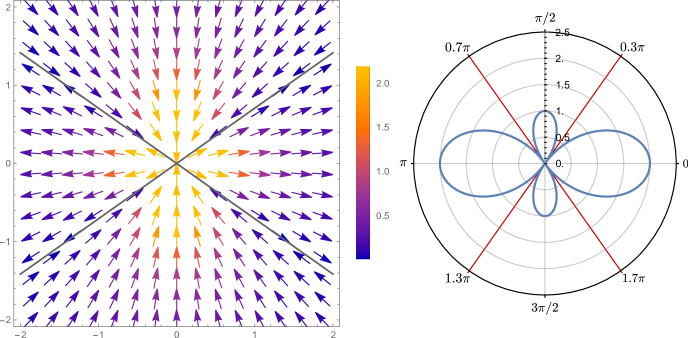
Figure 1: Magnetic field (21) produced in a constant background by the pointlike static charge. The background fields are directed along the vertical axis on the left panel while along the horizontal axis on the right panel. Left: Magnetic lines of force. Owing to the $r^{-2}$ dependence, arrow heads near the origin are bigger than those away from the origin. Red (blue) colors indicate higher (lower) intensities and the inclined lines mark regions of zero magnetic field. Right: Polar plot of (21). Magnetic flux is inflowing within the polar cones $0\leq\theta\leq\arccos\left(1/\sqrt{3}\right)$ and $\pi-\arccos\left(1/\sqrt{3}\right)\leq\theta\leq\pi$, and outflowing within $\arccos\left(1/\sqrt{3}\right)\leq\theta\leq\pi-\arccos\left(1/\sqrt{3}\right)$. In the plot, $\arccos\left(1/\sqrt{3}\right)\approx 0.3\pi$. The overall in- and out-flows compensate each other when integrated in (30) with the measure $\sin{\theta}d\theta$ within the limits $(0,\pi)$, thereby providing vanishing of magnetic charge.

The field (21) is singular in one point, similar to that of a magnetic monopole. It is radial in the sense it is parallel to the radius-vector $\mathbf{r}$, but not spherically symmetric, since it depends on the angle $\theta$ between the radius-vector and the (common) direction of the background fields.

The vector potential

$$\mathbf{A}^{\left(1\right)}\left(\mathbf{r}\right)=-\frac{q\mathfrak{\tilde{g}}}{8\pi}\frac{\left[\mathbf{\hat{z}}\times\mathbf{\hat{r}}\right]}{r}\cos\theta\,,$$ (32)

gives rise to the magnetic field (21) via the relation $\mathbf{B}^{\left(1\right)}\left(\mathbf{r}\right)=\boldsymbol{\nabla}\times\mathbf{A}^{\left(1\right)}\left(\mathbf{r}\right)$, the spatial component of $f^{(1)\mu\nu}(\mathbf{r})$. It obeys the Coulomb gauge condition $\mathbf{\nabla}\cdot\mathbf{A}^{\left(1\right)}\left(\mathbf{r}\right)=0$. In the gauge chosen, the potential has no singularity in the angle variable $\cos\theta=\zeta$. Therefore, nothing hinders the Bianchi identity (29) from being fulfilled.

In order to accurately address Eqs. (3), it is possible to regularize the point charge, just as we have done in our previous works [69, 71]. The solutions presented above are consistent with the limiting cases discussed in these references. The singular solutions discussed in the following section should be seen as a limit of solutions for nonlinear equations with an extended source of Coulomb field.

3 Solutions singular on a line

3.1 Electric fields

The Gauss (17) and Faraday (25) laws admit many more solutions apart from those discussed in the preceding section. The existence of extra solutions stems from an indeterminacy of boundary conditions to the Cauchy problem for the set of partial differential equations (17), (25). To find these solutions, we change to spherical coordinates, where $\mathbf{\hat{r}}$, $\boldsymbol{\hat{\theta}}$, and $\boldsymbol{\hat{\varphi}}$ denote, the radial, polar, and azimuthal spherical unit vectors, respectively, and seek for solutions in the form

$$\mathbf{E}\left(\mathbf{r}\right)=E_{r}\left(r,\theta\right)\mathbf{\hat{r}}+E_{\theta}\left(r,\theta\right)\boldsymbol{\hat{\theta}}\,.$$ (33)

Solutions of this sort exist because the induced charge density (22) depends on $r$ and $\theta$, only. From now on we omit for simplicity the superscript “$\left(1\right)$” by $\mathbf{E}\left(\mathbf{r}\right)$ indicating the first-order approximation to Eqs. (3) or (7), since no other approximation will be used. We only reserve this superscript as referred specially to field (20). In spherical coordinates, the components obey the set of first-order partial differential equations

$$\frac{1}{r}\partial_{r}\left(r^{2}E_{r}\right)+\frac{1}{\sin\theta}\partial_{\theta}\left(\sin\theta E_{\theta}\right)=\frac{q\mathfrak{b}}{4\pi}\frac{1-3\cos^{2}\theta}{r^{2}}\,,$$

$$\partial_{r}\left(rE_{\theta}\right)-\partial_{\theta}E_{r}=0\,,$$ (34)

where $\partial_{r}=\partial/\partial r$, $\partial_{\theta}=\partial/\partial\theta$. Sticking to solutions proportional to $\mathfrak{L}_{\mathfrak{F}}$, $\mathfrak{L}_{\mathfrak{G}}$, $\mathfrak{b}$, and $\mathfrak{\tilde{g}}$, electric responses (33) must depend on $r^{-2}$. Hence

$$E_{r}\left(r,\theta\right)=\frac{P\left(\theta\right)}{r^{2}}\,,\ \ E_{\theta}\left(r,\theta\right)=\frac{Q\left(\theta\right)}{r^{2}}\,,$$ (35)

whose angular parts obey the differential equations

$$Q^{\prime}+Q\cot\theta = \frac{q\mathfrak{b}}{4\pi}\left(1-3\cos^{2}\theta\right)\,,$$ (36)

$$P^{\prime}\left(\theta\right) = -Q\left(\theta\right)\,.$$ (37)

Solution to the first one is

$$Q\left(\theta\right)=-\frac{q\mathfrak{b}}{4\pi r^{2}}\cos\theta\sin\theta+\frac{\tilde{\varkappa}}{r^{2}\sin\theta},$$ (38)

where $\tilde{\varkappa}$ is an integration constant. The part, proportional to it in (38), makes an arbitrary-magnitude solution to the equation obtained from (36) by omitting the inhomogeneity, its right-hand side. When solving the other equation (37), we acquire another integration constant $\varkappa$ to be fixed below by a sort of boundary condition.

Finally, the electric response (33) has the general form

$$\mathbf{E}\left(\mathbf{r}|\varkappa,\tilde{\varkappa}\right)=\frac{q}{4\pi r^{2}}\left[\left(\varkappa-\frac{\mathfrak{b}}{2}\cos^{2}\theta\right)\mathbf{\hat{r}}-\mathfrak{b}\cos\theta\sin\theta\boldsymbol{\hat{\theta}}\right]+\tilde{\varkappa}\boldsymbol{\Upsilon}\left(\mathbf{r}\right)\,,$$ (39)

where

$$\boldsymbol{\Upsilon}\left(\mathbf{r}\right)=\Upsilon_{r}\left(r,\theta\right)\mathbf{\hat{r}}+\Upsilon_{\theta}\left(r,\theta\right)\boldsymbol{\hat{\theta}}\,,$$

$$\Upsilon_{r}\left(r,\theta\right)=-\frac{\ln\tan\theta/2}{r^{2}}\,,\ \ \Upsilon_{\theta}\left(r,\theta\right)=\frac{\csc\theta}{r^{2}}\,,\ \ 0<\theta<\pi\,.$$ (40)

Note that both constants $\varkappa$, $\tilde{\varkappa}$ are explicitly shown in the argument of the electric response to distinguish (39) from the field (20). Recall that electric fields are polar vectors under space reflections $\mathbf{r}\rightarrow-\mathbf{r}$ (or $r\rightarrow r$, $\theta\rightarrow\pi-\theta$, $\varphi\rightarrow\varphi+\pi$, in spherical coordinates). This property implies that $\tilde{\varkappa}$ is a pseudoscalar while $\varkappa$ is a scalar (note that $\cos\theta$, too, changes sign under reflection: $\cos\theta\rightarrow-\cos\theta$, so does $\ln\tan\theta/2$). In the present problem, the pseudoscalar constant is supplied by the nonlinearity to be $\mathfrak{\tilde{g}}$ (14) or/and $\mathfrak{L}_{\mathfrak{G}}$. Constant $\tilde{\varkappa}$ may be thought of as a linear function of $\mathfrak{L}_{\mathfrak{G}}$ and $\mathfrak{\tilde{g}}$ with arbirary numerical coefficients.

The integration constant $\varkappa$ is determined to be $\varkappa=\mathfrak{L}_{\mathfrak{F}}+\mathfrak{b}/2$ by integrating Eq. (17) over a spherical surface $S$ of arbitrary radius with its center in $r=0$:

$$\oint_{S}\left[\mathbf{E}\left(\mathbf{r}|\varkappa,\tilde{\varkappa}\right)-\boldsymbol{\mathfrak{E}}^{(0)}\left(\mathbf{r}\right)\right]\cdot\mathbf{\hat{n}}dS=0\therefore\varkappa=\mathfrak{L}_{\mathfrak{F}}+\frac{\mathfrak{b}}{2}\,.$$ (41)

Therefore, we have rederived (by different method and in different coordinates) the electric response (20) and found its generalization (39), that differs from (20) by the term parameterized by $\tilde{\varkappa}$

$$\mathbf{E}\left(\mathbf{r}|\tilde{\varkappa}\right)=\mathbf{E}^{\left(1\right)}\left(\mathbf{r}\right)+\tilde{\varkappa}\boldsymbol{\Upsilon}\left(\mathbf{r}\right)\,,$$ (42)

that remains an unfixed integration constant, since it does not contribute to the surface integral (41) and thereof to the total charge. The integration constant $\tilde{\varkappa}$ is to be chosen from among any of pseudoscalars found within the model, multiplied by arbitrary number. As long as angle-singular solutions should disappear when the background field approaches zero, in parity-even theories $\tilde{\varkappa}$ may be proportional to $\mathfrak{L}_{\mathfrak{G}}$ and/or to the combinations $\overline{\mathfrak{G}}\mathfrak{L}_{\mathfrak{FF}}$, $\overline{\mathfrak{G}}\mathfrak{L}_{\mathfrak{GG}}$, and $\overline{\mathfrak{F}}\mathfrak{L}_{\mathfrak{FG}}$ that are dimensionally appropriate. For special parity-violating theories, this constant may depend on $\mathfrak{L}_{\mathfrak{F}}$ and/or combinations on $\overline{\mathfrak{G}}\mathfrak{L}_{\mathfrak{FG}}$ and $\overline{\mathfrak{F}}\mathfrak{L}_{\mathfrak{FF}}$, $\overline{\mathfrak{F}}\mathfrak{L}_{\mathfrak{GG}}$ , since these are now odd in pseudoscalar $\overline{\mathfrak{G}}=-\overline{\mathbf{E}}\cdot\overline{\mathbf{B}}$. Note that the first term in the right-hand-side of (42) coincides with the electric response (20). Also, the radial and angular components of $\boldsymbol{\Upsilon}\left(\mathbf{r}\right)$ are, in accord with (37), connected as

$$\ln\tan\theta/2=\int_{\pi/2}^{\theta}\csc\theta^{\prime}d\theta^{\prime}\,.$$ (43)

The $\tilde{\varkappa}$-part of the electric response (42), $\tilde{\varkappa}\boldsymbol{\Upsilon}\left(\mathbf{r}\right)$, is singular on the $z$-axis (i.e., at $\theta=0$, $\theta=\pi$), and in the origin, $\mathbf{r}=\mathbf{0}$. Outside the singularities, the charge density supporting this field disappears

$$\boldsymbol{\nabla}\cdot\boldsymbol{\Upsilon}\left(\mathbf{r}\right)=0\,,\ \text{ }0<\theta<\pi\,.$$ (44)

Thus, the field $\boldsymbol{\Upsilon}\left(\mathbf{r}\right)$ is a free solution there and, correspondingly, it has arbirary magnitude. Notice that the identity (44) is also valid at $\mathbf{r}=0$ because no charge supporting the field $\boldsymbol{\Upsilon}\left(\mathbf{r}\right)$ is concentrated at the origin. This fact follows from the triviality of the Gauss theorem

$$\int_{V}\boldsymbol{\nabla}\cdot\boldsymbol{\Upsilon}\left(\mathbf{r}\right)d\mathbf{r}=\oint_{S}\boldsymbol{\Upsilon}\left(\mathbf{r}\right)\cdot\mathbf{\hat{n}}dS=0\,,$$ (45)

applied to any sphere $S$ of arbitrary radius centered at the singularity point $\mathbf{r}=\mathbf{0}$. In other words, the charge density supporting the singular field (40) comes entirely from the $z$-axis, as shall be seen below.

To extend the divergence (44) to the $z$-axis ($\theta=0$, $\theta=\pi$), consider the outward flux of $\boldsymbol{\Upsilon}\left(\mathbf{r}\right)$ through the surface of an infinitesimally short conic cylinder coaxial with this axis, whose arc-like bases lie at $r$ and $r+\Delta r$, $\Delta r\ll r$, while the side wall has its angular coordinate $\theta$. Once $\Upsilon_{r}\left(r,\theta\right)dS_{r}=\Upsilon_{r}\left(r,\theta\right)r^{2}\sin\theta d\theta d\varphi$ is independent of $r$ according to (40), the fluxes through the two bases cancel one another and we are left with the flux through the wall alone

$$\oint_{S_{cc}}\boldsymbol{\Upsilon}\left(\mathbf{r}\right)\cdot\mathbf{\hat{n}}dS = 2\pi\int_{r}^{r+\Delta r}\Upsilon_{\theta}\left(r^{\prime},\theta\right)r^{\prime}\sin\theta dr^{\prime}$$ (46)

$$= 2\pi\Delta r\Upsilon_{r}\left(r,\theta\right)r\sin\theta=2\pi\frac{\Delta r}{r}\,,$$

in which Eq. (40) has been used in the last row. This relates to the upper hemisphere ($\mathbf{\hat{r}}\geq 0$, $\boldsymbol{\hat{\theta}}\geq 0$). The flux (46) does not depend on $\theta$, which is expected, since the integration surface can be deformed without affecting the flux – unless it crosses axis $z$ – due to the vanishing of divergence (44). Hence, the value $\theta=0$ may be attributed to (46). Then in the half-space of positive $z$, it holds that $r=z$, $\Delta r=\Delta z$, and charge is distributed along positive half-axis $z$ with the linear density

$$\frac{\tilde{\varkappa}\oint_{S_{cc}}\boldsymbol{\Upsilon}\left(\mathbf{r}\right)\cdot\mathbf{\hat{n}}dS}{\Delta z}=\frac{2\pi\tilde{\varkappa}}{z}\,,$$ (47)

inversely proportional to the distance from the seeded charge $q$. The volume density of charge $\rho_{\mathrm{di-thr}}\left(\mathbf{r}|\tilde{\varkappa}\right)$ may be written as

$$\tilde{\varkappa}\boldsymbol{\nabla}\cdot\boldsymbol{\Upsilon}\left(\mathbf{r}\right)=\frac{2\pi\tilde{\varkappa}}{z}\delta\left(\mathbf{r}_{\perp}\right)=\rho_{\mathrm{di-thr}}\left(\mathbf{r}|\tilde{\varkappa}\right)\,,\ \ \delta\left(\mathbf{r}_{\perp}\right)=\delta\left(x\right)\delta\left(y\right)\,,$$ (48)

so that the volume integral over the above conic cylinder, via the Gauss theorem, be
$\tilde{\varkappa}\int_{z}^{z+\Delta z}\boldsymbol{\nabla}\cdot\boldsymbol{\Upsilon}\left(\mathbf{r}\right)dz\int dxdy=2\pi\tilde{\varkappa}\Delta z/z$ in agreement with the flux (47). The factor $2\pi$ may be omitted in view of arbitrariness of $\tilde{\varkappa}$. It can be shown that Eq. (48) retains its form at negative $z$ as well, which fact is in accord with the nullification of the total charge in the whole space, explained above (after eq. (40)). Therefore, the signs of the charge of the thread are opposite at opposite sides of the point $z=0$. This suggests the name “di-thread” by analogy with “dipole”. The pattern of lines of force is shown in Fig. 2. These are formed by arcs, starting from the positive $z$-axis and ending on the negative $z$-axis. Note that, once $1/z$ reverses sign under space reflection, the charge density (48) is a scalar function in agreement with the condition that the divergence of electric field must result in a scalar function.

To conclude, Eq. (48) is our promised extension of relation (44) to include axis $z$. The background of parallel external constant magnetic and electric fields perturbed by a seeded point charge predisposes to considering exotic charged di-thread and electric field produced by it by supplying a pseudoscalar constant necessary to form the charge – the same as to form magnetic charge in the next Section and, generally, in nature as well.

The issue is quite similar to the standard point-like charge $Q$ in Maxwell’s electrodynamics. Outside the origin $\mathbf{r}=\mathbf{0}$, where the point charge is located, its electric field obeys the free equation $\boldsymbol{\nabla}\cdot\mathbf{E}\left(\mathbf{r}\right)=0$, whose solution (decreasing in the far-off domain) is $\mathbf{E}\left(\mathbf{r}\right)=\left(Q/4\pi r^{3}\right)\mathbf{r}$, where $Q$ arises as an arbitrary integration constant to be identified with the charge that supports the field. Its role is analogous to that of our integration constant $\tilde{\varkappa}$ that determines the magnitude of the charge of the di-thread (48).

Similar to the point charge $Q$, the charge density of the di-thread (48) should be understood as an externally given parameter, in contrast to the induced charge density (22) which depends exclusively on the seeded charge $q$. Correspondingly, the thread density  $A^{0}\left(\mathbf{r}\right)\rho_{\mathrm{di-thr}}\left(\mathbf{r}|\tilde{\varkappa}\right)$ should be added to Lagrangian in the action (2) and appear in the right-hand side of the equation in place of (17); cf. analogous statement concerning Dirac string current in the next Section.

To conclude this section, we emphasize that the Bianchi identity

$$\boldsymbol{\nabla}\times\boldsymbol{\Upsilon}\left(\mathbf{r}\right)=\mathbf{0}\,,$$ (49)

holds everywhere, including at the singularities $\mathbf{r}=\mathbf{0}$, $\theta=0$, and $\theta=\pi$. This result follows from the triviality of the Stokes theorem

$$\int_{\mathcal{S}}\left[\boldsymbol{\nabla}\times\boldsymbol{\Upsilon}\left(\mathbf{r}\right)\right]\cdot\mathbf{\hat{n}}d\mathcal{S}=\oint_{\mathcal{C}}\boldsymbol{\Upsilon}\left(\mathbf{r}\right)\cdot d\mathbf{l}=0\,,$$ (50)

applied to any closed contour $\mathcal{C}$  enclosing the origin and any segment of the $z$-axis. To reach this conclusion, we calculated the integral on the right for two different contours. The first was a circle of arbitrary radius, centered at the $z$-axis and perpendicular to it. This circle could be placed at any height with respect to the $xy$-plane. The second contour was a rectangle of any shape, located at a plane with $\mathbf{r}_{\perp}=\mathrm{const.}$, enclosing the origin (but not passing through it) and a segment of the $z$-axis. In the first case, the line integral in (50) is identically zero because the field $\boldsymbol{\Upsilon}\left(\mathbf{r}\right)$ is always perpendicular to the unit vector tangent to the circle $d\mathbf{l}=\left|\mathbf{r}_{\perp}\right|d\varphi\boldsymbol{\hat{\varphi}}$ , i.e., $\boldsymbol{\Upsilon}\left(\mathbf{r}\right)\cdot d\mathbf{l}=0$, where $\left|\mathbf{r}_{\perp}\right|=\sqrt{x^{2}+y^{2}}$ denotes the magnitude of the polar radius and $\varphi\in\left[0,2\pi\right)$ the polar angle. As for the rectangular contour, the line integral vanishes identically, regardless the size of the rectangle. This identity can be straightforwardly shown using the representation of $\boldsymbol{\Upsilon}\left(\mathbf{r}\right)$ in Cartesian coordinates,

$$\boldsymbol{\Upsilon}\left(\mathbf{r}\right) = \Upsilon_{\perp}\left(\mathbf{r}\right)\mathbf{\hat{r}}_{\perp}+\Upsilon_{\parallel}\left(\mathbf{r}\right)\mathbf{\hat{z}}\,,\ \ \mathbf{\hat{r}}_{\perp}=\frac{x\mathbf{\hat{x}}+y\mathbf{\hat{y}}}{\left|\mathbf{r}_{\perp}\right|}\,,$$

$$\Upsilon_{\perp}\left(\mathbf{r}\right) = \frac{1}{\mathbf{r}_{\perp}^{2}+z^{2}}\left(\frac{z}{\left|\mathbf{r}_{\perp}\right|}-\frac{\left|\mathbf{r}_{\perp}\right|}{2\sqrt{\mathbf{r}_{\perp}^{2}+z^{2}}}\ln\frac{\sqrt{\mathbf{r}_{\perp}^{2}+z^{2}}-z}{\sqrt{\mathbf{r}_{\perp}^{2}+z^{2}}+z}\right)\,,$$

$$\Upsilon_{\parallel}\left(\mathbf{r}\right) = -\frac{1}{\mathbf{r}_{\perp}^{2}+z^{2}}\left(1+\frac{z}{2\sqrt{\mathbf{r}_{\perp}^{2}+z^{2}}}\ln\frac{\sqrt{\mathbf{r}_{\perp}^{2}+z^{2}}-z}{\sqrt{\mathbf{r}_{\perp}^{2}+z^{2}}+z}\right)\,.$$ (51)

As a result, no current flux through the origin and the z-axis exists, which means that the singular field is a pure gradient field

$$\boldsymbol{\Upsilon}\left(\mathbf{r}\right)=-\boldsymbol{\nabla}\Xi\left(\mathbf{r}\right)\,,\ \ \Xi\left(\mathbf{r}\right)=-\frac{\ln\tan\theta/2}{r}+\tilde{\xi}\,,$$ (52)

everywhere. Here, $\tilde{\xi}$ is a pseudoscalar constant. In other words, the electric field (42) respects the Bianchi identity (15) at all points, $\boldsymbol{\nabla}\times\mathbf{E}\left(\mathbf{r}|\tilde{\varkappa}\right)=\mathbf{0}$. Notice that the potential $\Xi\left(\mathbf{r}\right)$ is a pseudoscalar function, as it should be since $\boldsymbol{\Upsilon}\left(\mathbf{r}\right)$ is a space-reflection invariant vector field. Thus, up to an unimportant constant, the singular part of $\mathbf{E}^{\left(1\right)}\left(\mathbf{r}|\tilde{\varkappa}\right)$ can be written as the gradient of the scalar potential

$$A_{0}\left(\mathbf{r}|\tilde{\varkappa}\right)=A_{0}^{\left(1\right)}\left(\mathbf{r}\right)+\tilde{\varkappa}\Xi\left(\mathbf{r}\right)\,,$$ (53)

where the first term is given by Eq. (26). It should be noted that just like the singular field $\tilde{\varkappa}\boldsymbol{\Upsilon}\left(\mathbf{r}\right)$, the scalar potential $\tilde{\varkappa}\Xi\left(\mathbf{r}\right)$is also singular at the $z$-axis, the origin $\mathbf{r}=\mathbf{0}$ included.

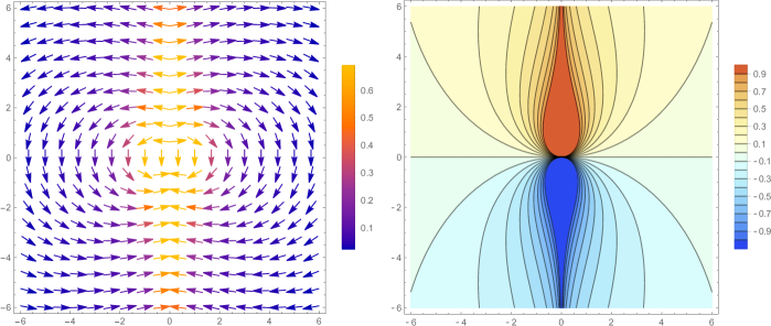
Figure 2: Projections of the lines of force of the singular field $\boldsymbol{\Upsilon}\left(\mathbf{r}\right)$ (40) (left panel) and its equipotential curves $\Xi\left(\mathbf{r}\right)$ (52) (solid lines, right panel) on the $yz$-plane. On the left panel, the horizontal axis denotes the $y$-component of the field, $\Upsilon_{y}\left(0,y,z\right)$, while the vertical denotes the $z$-component, $\Upsilon_{z}\left(0,y,z\right)$. The intensity of the field and the potential are reflected by the color scheme dictated the labels on the right of each plot.

3.2 Magnetic fields

In contrast to the magnetically neutral magnetic field (21) created in a constant two-field background by a small point-like Coulomb source, we discuss below a magnetic solution to the same field equation, which carries a nontrivial magnetic charge. Similarly to the electric solutions, the linearized Maxwell’s equations for magnetic ones (18) admit more solutions apart from those considered in Sec. 2. Firstly, we seek for solutions in the non-radial, angle-dependent form

$$\mathbf{B}\left(\mathbf{r}\right)=B_{r}\left(r,\theta\right)\mathbf{\hat{r}}+B_{\theta}\left(r,\theta\right)\boldsymbol{\hat{\theta}}\,,$$ (54)

and rewrite the Maxwell equations (18), (29) in spherical coordinates to learn that the components obey the set of equations

$$\partial_{r}\left(rB_{\theta}\right)-\partial_{\theta}B_{r}=-\frac{3\mathfrak{\tilde{g}}q}{4\pi}\frac{\cos\theta\sin\theta}{r^{2}}\,,$$

$$\partial_{\theta}\left(\sin\theta B_{\theta}\right)+\frac{1}{r}\partial_{r}\left(r^{2}B_{r}\right)=0\,.$$ (55)

Notice that we omitted the superscript “$\left(1\right)$” by $\mathbf{B}\left(\mathbf{r}\right)$ in (54) to avoid confusion with the magnetic response (21). We adopt this convention from now on.

Restricting to magnetic solutions proportional to $\mathfrak{L}_{\mathfrak{F}}$, $\mathfrak{L}_{\mathfrak{G}}$, $\mathfrak{b}$, and $\mathfrak{\tilde{g}}$, the fields (54) must depend on the radial coordinate as $r^{-2}$,

$$B_{r}\left(r,\theta\right)=\frac{J\left(\theta\right)}{r^{2}}\,,\ \ B_{\theta}\left(r,\theta\right)=\frac{K\left(\theta\right)}{r^{2}}\,.$$ (56)

Then, plugging the ansatzes (56) into Eqs. (55) we find

$$\partial_{\theta}\left(K\sin\theta\right)=0\,,\ \ J^{\prime}+K=\frac{3q\mathfrak{\tilde{g}}}{4\pi}\cos\theta\sin\theta\,.$$ (57)

Solving the first equation in (57) supplies the angular component with an arbitrary constant: $K\left(\theta\right)=\kappa\csc\theta$, $\kappa=\mathrm{const}$. Plugging this solution into the equation for $J\left(\theta\right)$ we finally obtain

$$\mathbf{B}\left(\mathbf{r}|\tilde{\kappa},\kappa\right)=\mathbf{B}_{\mathrm{ch}}\left(\mathbf{r}|\tilde{\kappa}\right)+\kappa\boldsymbol{\Upsilon}\left(\mathbf{r}\right)\,,$$ (58)

where $\tilde{\kappa}$ is another integration constant, stemming from the equation for $J\left(\theta\right)$ in (57), the vector field $\boldsymbol{\Upsilon}\left(\mathbf{r}\right)$ was defined before (40), and

$$\mathbf{B}_{\mathrm{ch}}\left(\mathbf{r}|\tilde{\kappa}\right)=\left(\tilde{\kappa}-\frac{3q\mathfrak{\tilde{g}}}{8\pi}\cos^{2}\theta\right)\frac{\mathbf{\hat{r}}}{r^{2}}\,.$$ (59)

Following the same arguments that led to Eq. (42), i.e., appealing to the fact that magnetic fields are axial vectors, we conclude that $\tilde{\kappa}$ is a pseudoscalar while $\kappa$ is a scalar. Magnetic field (58) contains the response (21) in itself, bearing in mind that $\tilde{\kappa}$ is arbitrary. $\mathbf{B}_{\mathrm{ch}}\left(\mathbf{r}|\tilde{\kappa}\right)$ is radial, whereas $\kappa\boldsymbol{\Upsilon}\left(\mathbf{r}\right)$ depends on $\theta$. Notice that we regain the magnetic response (21) from (59) by choosing $\tilde{\kappa}=q\mathfrak{\tilde{g}}/8\pi$; i.e., $\mathbf{B}_{\mathrm{ch}}\left(\mathbf{r}|q\mathfrak{\tilde{g}}/8\pi\right)=\mathbf{B}^{\left(1\right)}\left(\mathbf{r}\right)$.

Unlike the electric solutions (42), magnetic solutions found above are twice arbitrary because both constants remain undetermined by the consistency with the Bianchi identity (29) and the induced current density Eq. (27). It should be noted that $\boldsymbol{\nabla}\times\mathbf{B}\left(\mathbf{r}|\tilde{\kappa},\kappa\right)=\boldsymbol{\nabla}\times\mathbf{B}^{(1)}\left(\mathbf{r}\right)$ beyond the singularities, hence the solutions (58) may be alternatively presented as

$$\mathbf{B}\left(\mathbf{r}|\tilde{\kappa},\kappa\right)=\mathbf{B}^{\left(1\right)}\left(\mathbf{r}\right)+\boldsymbol{\nabla}\Omega\left(\mathbf{r}|\tilde{\kappa}\right)-\kappa\boldsymbol{\nabla}\Xi\left(\mathbf{r}\right)\,,$$ (60)

where $\Omega\left(\mathbf{r}|\tilde{\kappa}\right)$ is the pseudoscalar potential

$$\Omega\left(\mathbf{r}|\tilde{\kappa}\right)=-\frac{1}{r}\left(\tilde{\kappa}-\frac{q\mathfrak{\tilde{g}}}{8\pi}\right)+\tilde{\omega}\,,$$

$\tilde{\omega}$ is a pseudoscalar constant, and $\Xi\left(\mathbf{r}\right)$ is defined in Eq. (52).

We shall be interested first in the radial solutions of equation (58), for which the pseudoscalar constant $\tilde{\kappa}$ may be formed by parameters of our problem: (dimensionally consistent) pseudoscalar combinations of the field invariants $\overline{\mathfrak{G}}$, $\overline{\mathfrak{F}}$, the derivatives $\mathfrak{L}_{\mathfrak{G}}$, $\mathfrak{L}_{\mathfrak{FG}}$, included. It must be noted that usual electrodynamics in the vacuum does not provide such a constant pseudoscalar. The Bianchi identity (29)

$$\boldsymbol{\nabla}\cdot\mathbf{B}_{\mathrm{ch}}\left(\mathbf{r}|\tilde{\kappa}\right)=0\,,\ \ \mathbf{r}\neq\mathbf{0}\,,$$ (61a)

is fulfilled everywhere, but not at the origin $$\mathbf{r}=\mathbf{0}$$. In other words, the magnetic charge is concentrated in a point. Its value is defined by the surface integral

$$q_{M}=\oint_{S}\left(\mathbf{B}_{\mathrm{ch}}\left(\mathbf{r}|\tilde{\kappa}\right)\cdot\mathbf{\hat{n}}\right)dS=4\pi\tilde{\kappa}-\frac{q\mathfrak{\tilde{g}}}{2}\,,$$ (62)

wherein the surface $S$ embracing the charge may be chosen as a sphere of arbitrary radius.

Following Gauss’ theorem $\oint_{S}\left(\mathbf{B}_{\mathrm{ch}}\left(\mathbf{r}|\tilde{\kappa}\right)\cdot\mathbf{\hat{n}}\right)dS=\int_{V}\left[\boldsymbol{\nabla}\cdot\mathbf{B}_{\mathrm{ch}}\left(\mathbf{r}|\tilde{\kappa}\right)\right]d^{3}x$, one unites (61a) and (62) in the form

$$\boldsymbol{\nabla}\cdot\mathbf{B}_{\mathrm{ch}}\left(\mathbf{r}|\tilde{\kappa}\right)=q_{M}\delta\left(\mathbf{r}\right)\,.$$ (63)

It is noteworthy that $\tilde{\kappa}$ is not arbitrary, as the magnetic charge must vanish in the limit of zero background. This requirement imposes certain restrictions on $\tilde{\kappa}$. For example, this constant could depend on $\mathfrak{L}_{\mathfrak{G}}$ and/or dimensionally consistent combinations of $\overline{\mathfrak{F}}$ with $\mathfrak{L}_{\mathfrak{FG}}$ and of $\overline{\mathfrak{G}}$ with $\mathfrak{L}_{\mathfrak{FF}}$, $\mathfrak{L}_{\mathfrak{GG}}$. In the special case of a P-odd theory, the magnetic charge may exist with no electric field in the background. Indeed, with $\overline{\mathbf{E}}=\overline{\mathfrak{G}}=0$, one finds that the remaining coefficients $\mathfrak{L}_{\mathfrak{FG}}$ and $\mathfrak{L}_{\mathfrak{G}}$ are zero, unless the Lagrangian itself contains a parity-violating term $\chi\left(\mathfrak{F}\right)\overline{\mathfrak{G}}$ linear in $\overline{\mathfrak{G}}$, so that $\mathfrak{L}_{\mathfrak{FG}}=\chi^{\prime}\left(\mathfrak{F}\right)\neq 0$, $\mathfrak{L}_{\mathfrak{G}}=\chi\left(\mathfrak{F}\right)\neq 0$. Moreover, in the limit of small constant fields, when we must set $\overline{\mathbf{E}}=\overline{\mathbf{B}}=0$ inside the coefficient functions, one has in a parity-even theory $\mathfrak{L}_{\mathfrak{G}}=\mathfrak{L}_{\mathfrak{FG}}=0$. In this case, Eq. (21) (or Eq. (59), with $\tilde{\kappa}=q\mathfrak{\tilde{g}}/8\pi$) coincides with the solution numbered as (12) in our previous paper [72] taken in the limit $b=0$. Note that the approximation exploited in [72] is different from that in the present paper, as commented above Eq. (7).

It remains to consider the last portion of the magnetic solution (58), proportional to $\kappa$. According to the discussion in the preceding subsection, the singular field $\mathbf{\Upsilon}\left(\mathbf{r}\right)$ is supported by a charge density concentrated on the $z$-axis and symmetrically distributed with positive/negative signs along the positive/negative semi-axes (48). This means that in addition to the magnetic charge (62), the magnetic field (58) is supported by a magnetic di-thread – a generalization of a magnetic dipole – owing to $\kappa\mathbf{\Upsilon}\left(\mathbf{r}\right)$, whose density reads

$$\boldsymbol{\nabla}\cdot\left[\kappa\mathbf{\Upsilon}\left(\mathbf{r}\right)\right]=\frac{2\pi\kappa}{z}\delta\left(\mathbf{r}_{\perp}\right)\,.$$ (64)

This magnetic charge density is understood as an external agent to be included into the primary Lagrangian. Like the magnetic charge (63), the above charge density is a pseudoscalar function, as it should be since the magnetic field $\kappa\mathbf{\Upsilon}\left(\mathbf{r}\right)$ is an axial vector field, as seen from (40). It is important to note that the value of $\kappa$ is not arbitrary, since the non-radial singular part of the solution (60) should disappear when the background field approaches zero. If the nonlinearity of the theory is symmetric under space reflection, then $\kappa$ may include dimensionless parity-even products of $\overline{\mathfrak{G}}$ with $\mathfrak{L}_{\mathfrak{FG}}$ and of $\overline{\mathfrak{F}}$ with $\mathfrak{L}_{\mathfrak{FF}}$, $\mathfrak{L}_{\mathfrak{GG}}$. As for parity-violating theories, $\kappa$ may depend on dimensionless parity-even products of $\overline{\mathfrak{G}}$ with $\mathfrak{L}_{\mathfrak{FF}}$, $\mathfrak{L}_{\mathfrak{GG}}$ and of $\overline{\mathfrak{F}}$ with $\mathfrak{L}_{\mathfrak{FG}}$. The magnetic field lines are the same as the electric lines depicted in the left panel of Fig. 2.

3.2.1 Singular vector potential and the Dirac string

The vector potential

$$\mathbf{A}_{\mathrm{ch}}^{\left(\pm\right)}\left(\mathbf{r}|\tilde{\kappa}\right)=\frac{\sin\theta}{4\pi r}\left(-\frac{q\mathfrak{\tilde{g}}}{2}\cos\theta\pm\frac{q_{M}}{1\pm\cos\theta}\right)\boldsymbol{\hat{\varphi}}\,,$$ (65)

which satisfies the equation to be obtained from (18) by the formal substitution
$\mathbf{B}_{\mathrm{ch}}\left(\mathbf{r}|\tilde{\kappa}\right)=\boldsymbol{\nabla}\times\mathbf{A}_{\mathrm{ch}}^{\left(\pm\right)}\left(\mathbf{r}|\tilde{\kappa}\right)$, is singular on the negative/positive half-axis $\cos\theta=\mp 1$ drawn along the common direction $\mathbf{\hat{z}}$ of the background fields. The Coulomb gauge condition

$$\mathbf{\nabla}\cdot\mathbf{A}_{\mathrm{ch}}^{\left(\pm\right)}\left(\mathbf{r}|\tilde{\kappa}\right)=0,\text{ \ }\zeta\neq\mp 1\,,\ \ \mathbf{r}\neq\mathbf{0}\,,$$ (66)

is satisfied by (65) beyond the singularity line. Its extension to the singularity line leaves it as it is. Indeed, the flux $\oint_{\mathcal{S}}\mathbf{A}_{\mathrm{ch}}^{\left(\pm\right)}\left(\mathbf{r}|\tilde{\kappa}\right)\cdot\mathbf{\hat{r}}d\mathcal{S}$ through a sphere $\mathcal{S}$ of radius $r$ is identically zero. The reason is that the normal vector pointing out the sphere is just the radius vector $\mathbf{\hat{r}}$, which is orthogonal to $\boldsymbol{\hat{\varphi}}$, namely $\boldsymbol{\hat{\varphi}}\cdot\mathbf{\hat{r}}=0$. Analogously, the flux of $\mathbf{A}_{\mathrm{ch}}^{\left(\pm\right)}\left(\mathbf{r}|\tilde{\kappa}\right)$ through an infinitely long cylinder surrounding the lines of singularities is zero too, since (65) is tangent both to its walls and its base.

The potential (65) produces (59) outside the singular half-axes

$$\mathbf{B}_{\mathrm{ch}}\left(\mathbf{r}|\tilde{\kappa}\right)=\boldsymbol{\nabla}\times\mathbf{A}_{\mathrm{ch}}^{\left(\pm\right)}\left(\mathbf{r}|\tilde{\kappa}\right)\,,\ \text{ }\mathbf{r}\neq\mathbf{0},\ \text{ }\zeta\neq\mp 1\,,$$ (67)

but at the region of singularities it gives rise to singular magnetic fields – “string” magnetic fields $\mathbf{B}_{\mathrm{string}}^{\mp}\left(\mathbf{r}|\tilde{\kappa}\right)$. To compute these contributions, we may extend the above relation to the forbidden half-axis through Stokes’s theorem (recall that we choose the axis $z$ along the background field; the axes $x$ and $y$ make Cartesian coordinates in the orthogonal plane $\mathbf{r}_{\perp}=(x,y)$)

$$\oint_{\mathcal{C}_{\mp}}\mathbf{A}_{\mathrm{ch}}^{\left(\pm\right)}\left(\mathbf{r}|\tilde{\kappa}\right)\cdot d\mathbf{l}=\int_{\mathcal{S}_{\mp}}\left(\mathbf{B}_{\mathrm{string}}^{\mp}\left(\mathbf{r}|\tilde{\kappa}\right)\cdot\mathbf{\hat{z}}\right)dxdy\,,$$ (68)

where the integral on the left is taken along any of circles $\mathcal{C}_{\mp}$ (enclosing the corresponding open surfaces $\mathcal{S}_{\mp}$) with a vanishing radius, $\left|\mathbf{r}_{\perp}\right|=r\sin\theta=r\sqrt{1-\zeta^{2}}\rightarrow 0$ as $\zeta\rightarrow\mp 1$, about the half-axis of singularities $z\lessgtr 0$. Any of the two circles $\mathcal{C}_{\mp}$ is a section of a plane orthogonal to $z$ with the spherical surface, whose radius is $r$. The surface integral on the right may be taken over the part $\mathcal{S}_{\mp}$ of the orthogonal plane restricted by the said circle. The left-hand integral is calculated as follows (the part, nonsingular on the half-axis, does not contribute in the limit $\zeta\rightarrow\mp 1$):

$$\oint_{\mathcal{C}_{\mp}}\mathbf{A}_{\mathrm{ch}}^{\left(\pm\right)}\left(\mathbf{r}|\tilde{\kappa}\right)\cdot d\mathbf{l}=\frac{1}{4\pi}\oint_{\mathcal{C}_{\mp}}\frac{\sin\theta}{r}\left(-\frac{q\mathfrak{\tilde{g}}}{2}\cos\theta\pm\frac{q_{M}}{1\pm\cos\theta}\right)\boldsymbol{\hat{\varphi}}\cdot d\mathbf{l}=\pm q_{M}\,.$$ (69)

Eqs.(69), (68) establish the value of the flux of the extra part of the magnetic field concentrated on singular half-axes through the orthogonal plane (cf. the procedure in [73], [74] described for the Dirac monopole [75]; see also the review [76]. Significance of the string field was also revealed in [77]). To satisfy Eqs. (69), (68) we have to prescribe the following distributional expression to that “string” magnetic field. It has only one, $z$-th, component, and its magnitude is

$$\mathbf{B}_{\mathrm{string}}^{\mp}\left(\mathbf{r}|\tilde{\kappa}\right)=\pm q_{M}\Theta\left(\mp z\right)\delta\left(\mathbf{r}_{\perp}\right)\mathbf{\hat{z}\,},$$ (70)

where $\Theta$ is the Heaviside step function. Finally, Eq. (67) is extended to the singular half-axis as

$$\mathbf{B}_{\mathrm{ch}}\left(\mathbf{r}|\tilde{\kappa}\right)=\boldsymbol{\nabla}\times\mathbf{A}_{\mathrm{ch}}^{\left(\pm\right)}\left(\mathbf{r}|\tilde{\kappa}\right)=\mathbf{B}_{\mathrm{ch}}\left(\mathbf{r}|\tilde{\kappa}\right)+\mathbf{B}_{\mathrm{string}}^{\mp}\left(\mathbf{r}|\tilde{\kappa}\right)=\mathbf{B}_{\mathrm{ch}}\left(\mathbf{r}|\tilde{\kappa}\right)\pm q_{M}\Theta\left(\mp z\right)\delta\left(\mathbf{r}_{\perp}\right)\mathbf{\hat{z}}\,.$$

Contrary to the Dirac monopole, in our case the monopole solution (59) is not center-symmetric. P.A.-M. Dirac [78] came to his intriguing prediction about discreteness of the product of electric and magnetic charges, pursuing the goal of making the string invisible for electrons. That was an obligation imposed by gauge invariance, because gauge transformation is able to alter configuration of the string. After the Aharonov-Bohm effect [79] had been discovered, the string invisibility became questionable. In our context, the string appears correlated with the direction of the external field. The situation may be viewed upon as a spontaneous breakdown: the string direction may be any, but is fixed by an external agent, the background field. As long as the gauge symmetry has been broken, we are no longer free to change the string orientation by a gauge transformation, and we see no reason for invisibility of string and charge discretization either. Moreover, in the next Subsubsection we shall see that the string field (70) requires a solenoidal current (72) as its source, axis of solenoid being the string direction. Certainly, current is not a subject of gauge transformation. This means that to give a magnetic monopole is to give its place, its charge and (direction of the axis of) its string current. If we choose this direction differently, we define a different monopole. This remark does not exclude the possible achievement of charge quantization by considering discreteness of angular momentum of electromagnetic fields. Such endeavors are attracting attention, for analysis with the account of the Dirac string see [80].

3.2.2 String current

The usual trouble characteristic of the standard magnetic monopole of Maxwell electrodynamics cured only by passing to nonAbelian gauge theory [81], (see also [74], [82]) are shared by our magnetic monopole (except that ours comes in already equipped with the necessary pseudoscalar coefficient).

Indeed, the full magnetic field produced by vector-potential (65)

$$\mathbf{B}_{\mathrm{string}}^{\mp}\left(\mathbf{r}|\tilde{\kappa}\right)+\mathbf{B}_{\mathrm{ch}}\left(\mathbf{r}|\tilde{\kappa}\right)\,,$$ (71)

is not a solution to Eq. (18). This fact follows from the nontriviality of the current flowing around the infinitely thin cylinder

$$\mathbf{j}_{\mathrm{string}}^{\mp}\left(\mathbf{r}|\tilde{\kappa}\right)=\boldsymbol{\nabla}\times\mathbf{B}_{\mathrm{string}}^{\mp}\left(\mathbf{r}|\tilde{\kappa}\right)=\pm q_{M}\left[\mathbf{\hat{x}}\delta\left(x\right)\delta^{\prime}\left(y\right)-\mathbf{\hat{y}}\delta^{\prime}\left(x\right)\delta\left(y\right)\right]\Theta\left(\mp z\right)\,,$$ (72)

which is not compatible with the initial set of nonlinear equations (18). More precisely, by substituting (71) in place of $\mathbf{B}^{\left(1\right)}\left(\mathbf{r}\right)$ into Eq. (18) (with $\mathbf{j}^{\left(1\right)}\left(\mathbf{r}\right)$ defined by (27))

$$\boldsymbol{\nabla}\times\mathbf{B}^{\left(1\right)}\left(\mathbf{r}\right)=\boldsymbol{\nabla}\times\left[\mathbf{B}_{\mathrm{string}}^{\mp}\left(\mathbf{r}|\tilde{\kappa}\right)+\mathbf{B}_{\mathrm{ch}}\left(\mathbf{r}|\tilde{\kappa}\right)\right]=\mathbf{j}^{\left(1\right)}\left(\mathbf{r}\right)\,,$$

and bearing in mind that $\boldsymbol{\nabla}\times\mathbf{B}_{\mathrm{ch}}\left(\mathbf{r}|\tilde{\kappa}\right)=\mathbf{j}^{\left(1\right)}\left(\mathbf{r}\right)$, we come to the wrong relation $\boldsymbol{\nabla}\times\mathbf{B}_{\mathrm{string}}^{\mp}\left(\mathbf{r}|\tilde{\kappa}\right)=\mathbf{0}$ in disagreement with Eq. (72). In short, the inconsistency is nested in the fact that the string-encircling current (72), whose role is to guarantee the vanishing of the total magnetic flux, i.e., fulfillment of Bianchi identity, is not present in initial field equations, neither it is an induced current – unlike $\mathbf{j}^{\left(1\right)}\left(\mathbf{r}\right)$.

More comments on this point are in order. Suppose, we would work with field equations via vector-potentials from the very beginning to intrinsically guarantee the Bianchi identities. To this end, replace $\mathbf{B}^{\left(1\right)}\left(\mathbf{r}\right)$ by $\boldsymbol{\nabla}\times\mathbf{A}\left(\mathbf{r}\right)$ in Eq.(18). Then, referring to the gauge condition $\boldsymbol{\nabla}\cdot\mathbf{A}\left(\mathbf{r}\right)=0$, it becomes

$$\boldsymbol{\nabla}\times[\boldsymbol{\nabla}\times\mathbf{A}\left(\mathbf{r}\right)]=\boldsymbol{\nabla}^{2}\mathbf{A}\left(\mathbf{r}\right)=\mathbf{j}^{(1)}\left(\mathbf{r}\right)\,.$$ (73)

This inhomogeneous equation has $\mathbf{A}\left(\mathbf{r}\right)=\mathbf{A}^{\left(1\right)}\left(\mathbf{r}\right)$ Eq. (32) as its (uncharged) solution, while the homogeneous equation $\boldsymbol{\nabla}^{2}\mathbf{A}\left(\mathbf{r}\right)=\mathbf{0}$ does not have any monopole solution. As for $\mathbf{A}_{\mathrm{ch}}^{\left(\pm\right)}\left(\mathbf{r}|\tilde{\kappa}\right)$, it does not obey Eq.(73), but on the contrary

$$\boldsymbol{\nabla}\times[\boldsymbol{\nabla}\times\mathbf{A}_{\mathrm{ch}}^{\left(\pm\right)}\left(\mathbf{r}|\tilde{\kappa}\right)]=\boldsymbol{\nabla}^{2}\mathbf{A}_{\mathrm{ch}}^{\left(\pm\right)}\left(\mathbf{r}|\tilde{\kappa}\right)=\mathbf{j}^{(1)}\left(\mathbf{r}\right)+\mathbf{j}_{\mathrm{string}}^{\mp}\left(\mathbf{r}|\tilde{\kappa}\right)\,,$$

keeping in mind the gauge condition $\mathbf{\nabla}\cdot\mathbf{A}_{\mathrm{ch}}^{\left(\pm\right)}\left(\mathbf{r}|\tilde{\kappa}\right)=0$ fulfilled everywhere as explained below (66). Thus, the resulting magnetic solution satisfies the relation

$$\boldsymbol{\nabla}\times\left[\mathbf{B}_{\mathrm{string}}^{\mp}\left(\mathbf{r}|\tilde{\kappa}\right)+\mathbf{B}_{\mathrm{ch}}\left(\mathbf{r}|\tilde{\kappa}\right)\right]=\mathbf{j}^{(1)}\left(\mathbf{r}\right)+\mathbf{j}_{\mathrm{string}}^{\mp}\left(\mathbf{r}|\tilde{\kappa}\right)\,.$$

We see again that in the framework of pure vector-potential approach, the current $\mathbf{j}_{\mathrm{string}}^{\mp}\left(\mathbf{r}|\tilde{\kappa}\right)$ is not inherent in our primary (nonlinear Abelian) electrodynamics, either. Therefore, in order to support the magnetic monopole rigged by a Dirac string, whose role is to guarantee the vanishing of the total magnetic flux, i.e. fulfillment of Bianchi identity, it would be necessary to introduce additively the solenoidal current into the primary Lagrangian (2) as an additional external source $\mathbf{A}\left(\mathbf{r}\right)\cdot\mathbf{j}_{\mathrm{string}}^{\mp}\left(\mathbf{r}|\tilde{\kappa}\right)$.

4 Conclusions

Within a general nonlinear local electrodynamics (2), we have obtained static electric and magnetic fields created by an electric point-like charge $q$ placed in a background of arbitrarily strong constant electric, $\overline{\mathbf{E}}$, and magnetic, $\overline{\mathbf{B}}$, fields, parallel between themselves, by solving (the second pair of) the Maxwell equations linearized near the background and treated in the approximation of small nonlinearity, eqs. (17, 18).

The point-like charge $q$ excites an induced charge (22) and (27) current densities in the equivalent medium formed by the background and supplies the Maxwell equations with inhomogeneities. Hence corresponding solutions – eq. (20) for electric and eq. (21) for magnetic fields – are nothing but linear responses of the medium to the imposed charge $q$. Our formulas for responses are determined by coefficients that are derivatives of the nonlinear part of the Lagrangian (2) over field invariants, where the background values of the fields are meant to be substituted after the derivatives have been calculated. Electric response (20) is characterized by nonzero total charge (24), which is the screened seeded charge $q$, and by scalar combinations of external fields. Magnetic response eq. (21) is characterized by zero total magnetic charge and by pseudoscalar combinations of external fields. Both responses are radial, but depend upon the angle $\theta$ beetween the radius-vector and the direction of external fields; they are free of singularities upon a line, but have one in the point $r=0$ where charge $q$ is located. So are the scalar (26)  and vector (32) potentials.

There are other solutions – those to homogeneous counterparts of the Maxwell equations, eqs. (17, 18) – additive to the responses. These are determined by arbitrary integration constants. Electric one, eqs. (39), (40) requires an arbitrary pseudoscalar factor $\tilde{\varkappa}$, since $\boldsymbol{\Upsilon}\left(\mathbf{r}\right)$ is a pseudovector field. It is not radial and it has a angular singularity at $\theta=0,\pi$ apart from the pole in the origin $r=0$. The total electric charge is zero, but there is a charge concentrated on infinitely thin thread stretched along axis $\theta=0,\pi$, it has opposite signs above and below the origin. We call it di-thread. As usual, the integration constant – it is $\tilde{\varkappa}$ in the present context – is fixed by the charge with the help of Gauss’ theorem. Linear charge density (48) $\tilde{\varkappa}\boldsymbol{\nabla}\cdot\boldsymbol{\Upsilon}\left(\mathbf{r}\right)=2\pi\tilde{\varkappa}\delta\left(\mathbf{r}_{\perp}\right)/z=\rho_{\mathrm{di-thr}}\left(\mathbf{r}|\tilde{\varkappa}\right)$ is to be considered as external parameter and included into primary action. The scalar potential (26) also bears singularities at $r=0$ and $\theta=0,\pi$. The pattern of lines of force and equipotential lines is presented in Fig. 1.

Magnetic solution has two parts: radial and not radial. The radial part (59) is written  as a combination of the mentioned magnetic response (21) and a nonzero point-like magnetic monopole with charge $q_{M}$ (62), the latter being determined by arbitrary integration constant, a pseudoscalar $\widetilde{\kappa}$ and the pseudoscalar combination $\widetilde{g}$ of constant external fields. (The need of a pseudoscalar is clear already because the standard magnetic monopole field $\thicksim q_{M}\mathbf{r}/r^{3}$ must be a pseudovector, while $\mathbf{r}$ is a polar vector. Hence the experimental search of magnetic monopole is, in fact, a search of a pseudoscalar in nature. In our context, the latter is proposed by the scalar product of external electric and magnetic fields $\overline{\mathfrak{G}}=-\overline{\mathbf{B}}\cdot\overline{\mathbf{E}}$. It is the nonlinearity of electrodynamics that is apt for combining $\overline{\mathfrak{G}}$ with the deviation field when building a magnetic monopole). Radial magnetic solution (59) has a singularity in $r=0$. Following the Gauss theorem, we have in a standard way the magnetic charge density $\boldsymbol{\nabla}\cdot\mathbf{B}_{\mathrm{ch}}\left(\mathbf{r}|\tilde{\kappa}\right)=q_{M}\delta\left(\mathbf{r}\right)$. This relation violates the Bianchi identity in $r=0$. As a result, the vector potential (65) is singular at $\theta=0$ or at $\theta=\pi$ making Dirac string along any of the half-axes $\theta=0$ or $\theta=\pi$ . Calculating its circulation around a half-axis of singularity one finds, as usual, magnetic field in the string $\mathbf{B}_{\mathrm{string}}^{\mp}\left(\mathbf{r}|\tilde{\kappa}\right)=\pm q_{M}\Theta\left(\mp z\right)\delta\left(\mathbf{r}_{\perp}\right)\mathbf{\hat{z}}$, (70) and the solenoidal current (72) flowing around the string $\mathbf{j}_{\mathrm{string}}^{\mp}\left(\mathbf{r}|\tilde{\kappa}\right)=\boldsymbol{\nabla}\times\mathbf{B}_{\mathrm{string}}^{\mp}\left(\mathbf{r}|\tilde{\kappa}\right)=\pm q_{M}\left[\mathbf{\hat{x}}\delta\left(x\right)\delta^{\prime}\left(y\right)-\mathbf{\hat{y}}\delta^{\prime}\left(x\right)\delta\left(y\right)\right]\Theta\left(\mp z\right)$ to support the magnetic field inside it.

The nonradial part of the magnetic solution is dual to nonradial part of the electric solution and is given by the same pseudovector field $\boldsymbol{\Upsilon}\left(\mathbf{r}\right)$ (40), but this time with a scalar integration constant $\kappa$ as a factor $\mathbf{B}\left(\mathbf{r}|\kappa\right)=\kappa\boldsymbol{\Upsilon}\left(\mathbf{r}\right)$. This is again field of a thin thread carrying a distributed – now magnetic – charge (64) of both polarities, the total charge being zero. The pattern of magnetic lines of force of this magnetic di-thread is the same as the one presented in Fig.1 for electric lines of force.

Both, the magnetic charge density, the solenoidal current and thread density are external agents to be included into primary action.

Lastly, it should be emphasized that the solutions of linearized Maxwell’s equations (1) for fields studied above within the approximation of lowest order in the magnitude of nonlinearity have the singularity structure of $\mathcal{V}/r^{2}$, where $\mathcal{V}$ is a dimensionless quantity. As the iterative equation (7) does not include any dimensional constant in its coefficients, there is no other dimensional quantity except $r$ to form fields. Hence this structure will retain in approximation of every order, the summation in (5) touching only the numerator $\mathcal{V}$.

Data Availability Statement

Data sharing is not applicable to this article as no new data were created or analyzed in this study.

References

- [1] O. Klein, Z. Phys. 53, 157 (1929).
- [2] F. Sauter, Z. Phys. 69, 742 (1931).
- [3] W. Heisenberg and H. Euler, Z. Phys. 98, 714 (1936);
- [4] V. Weisskopf, Kong. Dans. Vid. Selsk. Math-fys. Medd. XIV, 6 (1936) [English translation in: Early Quantum Electrodynamics: A Source Book, A. I. Miller (University Press, Cambridge, 1994)].
- [5] H. Euler and B Köckel, Naturwiss. 23, 246 (1935).
- [6] J. S. Schwinger, Phys. Rev. 82, 664 (1951).
- [7] D. Strickland and G. Mourou, Opt. Commun. 56, 219 (1985).
- [8] M. Marklund and P. K. Shukla, Rev. Mod. Phys. 78, 591 (2006).
- [9] G.V. Dunne, Eur. Phys. J. D 55, 327 (2009).
- [10] A. Di Piazza, C. Müller, K. Z. Hatsagortsyan, and C. H. Keitel, Rev. Mod. Phys. 84, 1177 (2012).
- [11] R. Battesti and C. Rizzo, Rep. Prog. Phys. 76, 016401 (2013).
- [12] B. King and T. Heinzl, High Power Laser Sci. Eng. 4, e5 (2016).
- [13] T. Blackburn, Rev. Mod. Plasma Phys. 4, 5 (2020).
- [14] F. Karbstein, Particles 3, 39 (2020).
- [15] A. Gonoskov, T. G. Blackburn, M. Marklund, and S. S. Bulanov, Rev. Mod. Phys. 94, 045001 (2022).
- [16] A. Fedotov, A. Ilderton, F. Karbstein, B. King, D. Seipt, H. Taya, and G. Torgrimsson, Phys. Rep. 1010, 1 (2023).
- [17] A.A. Grib, S.G. Mamaev and V.M. Mostepanenko, Vacuum quantum effects in strong fields, Friedmann Laboratory, St. Petersburg, Russia (1994).
- [18] W. Greiner, B. Muller and J. Rafelski, Quantum Electrodynamics Of Strong Fields, (Springer, Berlin, 1985).
- [19] E. S. Fradkin, D. M. Gitman, and S. M. Shvartsman, Quantum Electrodynamics with Unstable Vacuum, (Springer, Berlin, 1991),
- [20] W. Dittrich and M. Reuter, Effective Lagrangians In Quantum Electrodynamics, Lect. Notes Phys. 220, 1 (Springer, Berlin, 1985).
- [21] W. Dittrich and H. Gies, Probing the quantum vacuum. Perturbative effective action approach in quantum electrodynamics and its application, Springer Tracts Mod. Phys. 166, 1 (2000).
- [22] G. V. Dunne, Heisenberg-Euler effective Lagrangians: basics and extensions, in I. Kogan memorial volume, from fields to strings: circumnavigating theoretical physics, M. Shifman, A. Vainshtein and J. Wheater eds., World Scientific, Singapore, pg. 445 (2005); Int. J. Mod. Phys. A 27, 1260004 (2012).
- [23] R. Ruffini, G. Vereshchagin and S.-S. Xue, Phys. Rept. 487, 1 (2010).
- [24] F. Gelis and N. Tanji, Prog. Part. Nucl. Phys. 87, 1 (2016).
- [25] M. Aaboud et al. (ATLAS Collaboration), Evidence for light-by-light scattering in heavy-ion collisions with the ATLAS detector at the LHC, arXiv:1702.01625. Published in Nature Physics (2017).
- [26] S.L. Adler, Ann. Phys. (N.Y.) 67, 599 (1971).
- [27] H. Gies, F. Karbstein, N. Seegert, Phys. Rev. D 93, 085034 (2016).
- [28] C. Thompson and R.C. Duncan, Mon. Not. R. Astron. Soc. 275, 255 (1995); D. Lai and E.E. Salpeter, Phys. Rev. A 52, 2611 (1995).
- [29] W. H. Furry, Phys. Rev. 81, 115 (1951).
- [30] Xing Fan et al., arXiv:1705.00495 (2017); G. Zavattini et al., EPJC, 78, 585Z (2018); S.R. Valluri et al., Mon. Not. R. Astron. Soc. 472, 2398 (2017); M. Diachenko, O. Novak, R. Kholodov, Ukr. J. Phys. 64, 181 (2019).
- [31] T. Erber, Rev. Mod. Phys. 38, 626 (1966); Z. Bialynicka-Birula and I. Bialynicki-Birula, Phys. Rev. D 2, 2341 (1970).
- [32] I. A. Batalin and A. E. Shabad, Zh. Eksp. Teor. Fiz. 60, 894 (1971) [Sov. Phys. JETP 33, 483 (1971)].
- [33] R.P. Mignani et al., Mon. Not. R. Astron. Soc. 465, 492 (2017).
- [34] S. Kruglov, Int. J. Mod. Phys. A33, 1850023 (2018), Grav. Cosmol. 25, 190 (2019).
- [35] C. M. Kim and S. P. Kim, Eur. Phys. J. C 83, 104 (2023); arXiv:2112.02460; arXiv:2308.15830.
- [36] ATLAS Collaboration, Nature Physics 13, 852 (2017).
- [37] J. Ellis, N. E. Mavromatos, and T. You, Phys. Rev. Lett. 118, 261802 (2017).
- [38] N. E. Mavromatos and V. A. Mitsou, Int. J. Mod. Phys. A 35, 2030012 (2020).
- [39] J. Ellis, N. E. Mavromatos, P. Roloff, and T. You, Eur. Phys. J. C 82, 634 (2022).
- [40] E. S. Fradkin and A. A. Tseytlin, Phys. Lett. 163B, 123 (1985).
- [41] C. V. Costa, D. M. Gitman, and A. E. Shabad, Phys. Scr. 90, 074012 (2015).
- [42] T. C. Adorno, D. M. Gitman , A. E. Shabad, and A. A. Shishmarev, Russian Physics Journal 59, 1775 (2017).
- [43] I. F. Ginzburg and A. Schiller, Phys. Rev. D 60, 075016 (1999).
- [44] L. N. Epele, H. Fanchiotti, C. A. G. Canal, V. A. Mitsou, and V. Vento, Eur. Phys. J. Plus 127, 60 (2012).
- [45] K. Colwell and J. Terning, JHEP 1603, 068 (2016).
- [46] N. E. Mavromatos and V. A. Mitsou, EPJ Web Conf. 164, 04001 (2017).
- [47] V. A. Mitsou (MoEDAL), J. Phys: Conf. Ser. 2375, 012002 (2022).
- [48] V. A. Mitsou (MoEDAL), PoS EPS-HEP2021 704 (2022).
- [49] E. Musumeci and V. A. Mitsou, PoS ICHEP2022 1025 (2023).
- [50] MoEDAL collaboration, JHEP 08, 067 (2016).
- [51] MoEDAL collaboration, Phys. Lett. B 782, 510 (2018).
- [52] MoEDAL collaboration, Phys. Rev. Lett. 123, 021802 (2019).
- [53] O. Gould and A. Rajantie, Phys. Rev. Lett. 119 241601 (2017).
- [54] A. Rajantie, Monopole-antimonopole pair production by magnetic fields, Phil. Trans. Roy. Soc. A 377, 20190333 (2019).
- [55] O. Gould, D. L. J. Ho, and A. Rajantie, Phys. Rev. D 100, 015041 (2019).
- [56] D. L. J. Ho, and A. Rajantie, Phys. Rev. D 101, 055003 (2020).
- [57] O. Gould, D. L. J. Ho, and A. Rajantie, Phys. Rev. D 104, 015033 (2021).
- [58] P. Gaete and J. A. Helayël-Neto, Eur. Phys. J. C 83, 128 (2023).
- [59] R. Essig et.al., arXiv:1311.0029.
- [60] S. Villalba-Chávez, A. E. Shabad, and C. Müller, Eur. Phys. J. C 81, 331 (2021).
- [61] J-F. Fortin and K. Sinha, JCAP 11, 020 (2019).
- [62] J. M. A. Paixão, L. P. R. Ospedal, M. J. Neves, and J. A. Helayël-Neto, JHEP 10, 160 (2022).
- [63] M. J. Neves, P. Gaete, L. P. R. Ospedal, J. A. Helayël-Neto, J. Phys. A: Math. Theor. 56, 415701 (2023).
- [64] D. M. Gitman and A. E. Shabad, Phys. Rev. D 86, 125028 (2012).
- [65] T. C. Adorno, D. M. Gitman, and A. E. Shabad, Eur. Phys. J. C 74, 2838 (2014).
- [66] T. C. Adorno, D. M. Gitman, and A. E. Shabad, Phys. Rev. D 89, 047504 (2014).
- [67] V.I. Ritus, in Issues in Intense-Field Quantum Electrodynamics, Proc. Lebedev Phys. Inst. 168, 5, Ed. V.L. Ginzburg (Nova Science Publ., New York , 1987).
- [68] M. Born and L. Infeld, Proc. R. Soc. A 144, 425 (1934).
- [69] T. C. Adorno, D. M. Gitman, and A. E. Shabad, Eur. Phys. J. C 80, 308 (2020).
- [70] T. C. Adorno, D. M. Gitman, and A. E. Shabad, arXiv:1710.00138v2 [hep-th] 30 Sep 2019.
- [71] T. C. Adorno, D. M. Gitman, and A. E. Shabad, Phys. Rev. D 93, 125031 (2016).
- [72] T. C. Adorno, D. M. Gitman, and A. E. Shabad, Phys. Rev. D 92, 041702(R) (2015).
- [73] R. Heras, Contemp. Phys. 59, 331 (2018).
- [74] Y. M. Shnir, Magnetic Monopoles, (Springer, Berlin 2005).
- [75] P.A.M. Dirac, Proc. R. Soc. London A 133, 60 (1931).
- [76] N. E. Mavromatos and V. A. Mitsou, Int. J. Mod. Phys. A 35, 2030012 (2020).
- [77] M. Dunia, T. J. Evans, and D. Singleton, Phys. Rev. D 103, 128501 (2021).
- [78] P. A. M. Dirac, Phys. Rev. 74, 817 (1948).
- [79] Y. Aharonov and D. Bohm, Phys. Rev. 115, 485 (1959); M. Peshkin and A. Tonomura, The Aharonov—Bohm Effect, Springer-Verlag, Berlin (1989).
- [80] M. Dunia, P.Q. Hung, D. Singleton, Eur. Phys. J. C 83, 487 (2023).
- [81] G. ’t Hooft, Nucl.Phys.B 79, 276 (1974), A. M. Polyakov, JETP Lett. 20, 194 (1974).
- [82] Rossi Sylvain, ETH Zürich, https://ethz.ch/content/dam/ethz/special-interest/phys/theoretical-physics/itp-dam/documents/gaberdiel/proseminar_fs2018/20_Rossi.pdf
- [83] S. Karki and B. Altschul, Phys. Rev. D 102, 035009 (2020).