Tracking Quintessence

Abstract

Tracking quintessence, in a spatially flat and isotropic space-time with a minimally coupled canonical scalar field and an asymptotically inverse power-law potential $V(\varphi)\propto\varphi^{-p}$, $p>0$, as $\varphi\rightarrow 0$, is investigated. This is done by introducing a new three-dimensional regular dynamical system, which enables a rigorous explanation of the tracking feature: 1) The dynamical system has a tracker fixed point $\mathrm{T}$ with a two-dimensional stable manifold that pushes an open set of nearby solutions toward a single tracker solution originating from $\mathrm{T}$. 2) All solutions, including the tracker solution and the solutions that track/shadow it, end at a common future attractor fixed point that depends on the potential. Thus, the open set of solutions that shadow the tracker solution share its properties during the tracking quintessence epoch. We also discuss similarities and differences of underlying mechanisms for tracking, thawing and scaling freezing quintessence, and, moreover, we illustrate with state space pictures that all of these types of quintessence exist simultaneously for certain potentials.

1 Introduction

In 1998 observations of type Ia supernovae indicated that the Universe is presently accelerating [1, 2]. Within the framework of General Relativity this cosmic acceleration implies that there exists an exotic energy component in the Universe, called dark energy, with an equation of state parameter satisfying $w_{\mathrm{DE}}<-1/3$. The simplest candidate for dark energy, apart from a cosmological constant, is a dynamical canonical scalar field $\varphi$, minimally coupled to gravity and with a potential $V(\varphi)$, referred to as quintessence, Caldwell et al. (1998) [3] (for reviews and references about quintessence, see e.g. Tsujikawa (2013) [4] and Bahamonde et al. (2018) [5]). At the present time the energy density of quintessence and matter are roughly of the same size ($\Omega_{\varphi}\approx 0.7$, $\Omega_{\mathrm{m}}\approx 0.3$) which raises the need to explain this near coincidence without specifying precise initial conditions. To address this difficulty Zlatev et al. (1999) [6], and Steinhardt et al. (1999) [7] showed that for potentials with the property $V(\varphi)\propto\varphi^{-p}$, $p>0$, as $\varphi\rightarrow 0$, the quintessence governing equations have a special solution they called a tracker solution since it attracts solutions that then track/shadow it for a wide range of initial conditions. A second property the tracker solution exhibit is that the scalar field equation of state parameter $w_{\varphi}$ is nearly constant in the matter-dominated epoch and less than $w_{\mathrm{m}}$, the equation of state parameter of the background matter. This implies that the energy density $\rho_{\mathrm{m}}$ decreases faster than $\rho_{\varphi}$ so that as the universe evolves from matter-domination $\rho_{\varphi}$ will catch up and overtake $\rho_{\mathrm{m}}$. Taken together these two properties go some way toward solving the coincidence problem. This type of evolution is referred to as tracking quintessence.

In this paper we give a description of tracking quintessence by means of a new regular dynamical systems framework that is valid for asymptotically inverse power-law potentials, $V(\varphi)\propto\varphi^{-p}$, $p>0$, as $\varphi\rightarrow 0$. We use our new regular dynamical systems framework to show that there exists a unique tracker solution with the properties of the heuristically defined tracker solution of Steinhardt and co-workers, originating from a new hyperbolic tracker fixed point. The fact that all the eigenvalues of this isolated fixed point have non-zero real parts makes it possible to i) explain the tracking feature and ii) obtain analytic approximate expressions for tracker solutions. Moreover, the global and regular structure of the state space shows explicitly a) the entire tracker solution and gives insight into the possible initial conditions which lead to solutions that approach the tracker fixed point and then track/shadow the tracker solution; b) that these models also give rise to thawing quintessence solutions, and that some potentials belonging to the present class simultaneously in addition give rise to co-existing scaling freezing quintessence solutions.

The outline of the paper is as follows. In the next section we derive the new regular dynamical system. In Section 3 we briefly review the tracker conditions of Steinhardt and co-workers [7, 6] and describe the general structure of the new state space, including the fixed points of the dynamical system that determine the intermediate and late time behaviour of the quintessence solutions. In Section 4 we give a general dynamical systems description of thawing, scaling freezing and tracking quintessence, focussing on the latter, and in Section 5 we give specific examples that illustrate the previous general discussion using three-dimensional state space figures and graphs of $w_{\varphi}$. Finally, there is a brief concluding Section 6.

2 A regular dynamical system for unbounded $\lambda$

Consider a spatially flat and isotropic Robertson-Walker spacetime with a source that consists of matter with an energy density $\rho_{\mathrm{m}}>0$ and pressure $p_{\mathrm{m}}=0$, which represents cold dark matter, and a minimally coupled canonical scalar field, $\varphi$, with a potential $V(\varphi)>0$, which results in the following energy density and pressure

$$\rho_{\varphi}=\frac{1}{2}\dot{\varphi}^{2}+V(\varphi),\qquad p_{\varphi}=\frac{1}{2}\dot{\varphi}^{2}-V(\varphi),$$ (1)

where an overdot represents the derivative with proper time $t$. For these models, the Raychaudhuri equation, the Friedmann equation, the non-linear Klein-Gordon equation, and the energy conservation law for matter with zero pressure, can be written as

$$\dot{H}+H^{2} =-\frac{1}{6}(\rho+3p),$$ (2a)

$$3H^{2} =\rho,$$ (2b)

$$\ddot{\varphi} =-3H\dot{\varphi}-V_{,\varphi},$$ (2c)

$$\dot{\rho}_{\mathrm{m}} =-3H\rho_{\mathrm{m}},$$ (2d)

where the Hubble variable is defined by $H=\dot{a}/a$, and the total energy density $\rho$ and pressure $p$ are given by

$$\rho=\rho_{\varphi}+\rho_{\mathrm{m}},\qquad p=p_{\varphi}.$$ (3)

Our dynamical system is based on three key quantities associated with the scalar field: the scalar field equation of state parameter $w_{\varphi}:=p_{\varphi}/\rho_{\varphi}$, the Hubble-normalized energy density $\Omega_{\varphi}$ and scalar field potential $\Omega_{V}$:

$$1+w_{\varphi} :=\frac{\rho_{\varphi}+p_{\varphi}}{\rho_{\varphi}}=\frac{\varphi^{\prime 2}}{3\Omega_{\varphi}},\quad\text{provided that}\quad\Omega_{\varphi}>0,$$ (4a)

$$\Omega_{\varphi} :=\frac{\rho_{\varphi}}{3H^{2}}=\frac{1}{6}\varphi^{\prime 2}+\Omega_{V},$$ (4b)

$$\Omega_{V} :=\frac{V}{3H^{2}}=\frac{1}{2}(1-w_{\varphi})\,\Omega_{\varphi},$$ (4c)

where a ^′ denotes the derivative with respect to $e$-fold time, $N:=\ln(a/a_{0})$, where $a$ is the cosmological scale factor and $a_{0}=a(t_{0})$ is its value at the present time, given by $N=0$. It follows from (1) and (4) and the assumed positivity of $V$ that

$$1+w_{\varphi}\geq 0,\qquad 1-w_{\varphi}>0.$$ (5)

When using equations (2) we will convert from proper time $t$ to $e$-fold time $N$ using

$$\partial_{t}=H\partial_{N},\quad\partial_{t}^{2}=H^{2}[\partial_{N}^{2}-(1+q)\partial_{N}],$$ (6)

where the deceleration parameter $q$ is defined by

$$1+q:=-\frac{\dot{H}}{H^{2}}.$$ (7)

In particular (2c) assumes the form

$$\varphi^{\prime\prime}+(2-q)\varphi^{\prime}-3\lambda(\varphi)\Omega_{V}=0,$$ (8)

where $\lambda(\varphi)$ is defined by

$$\lambda:=-\frac{V_{,\varphi}}{V}.$$ (9)

We also need the Hubble-normalized matter density $\Omega_{\mathrm{m}}$ and its evolution equation, given by

$$\Omega_{\mathrm{m}}:=\frac{\rho_{\mathrm{m}}}{3H^{2}}=1-\Omega_{\varphi},\qquad\Omega_{\mathrm{m}}^{\prime}=(2q-1)\Omega_{\mathrm{m}},$$ (10)

as follows from (2d) and (7). The deceleration parameter $q$ can be expressed as

$$1+q=\frac{3}{2}\left(1+w_{\varphi}\Omega_{\varphi}\right),$$ (11)

as follows from (7) in conjunction with (1), (2) and (3).

Equation (4a), which can be written as

$$(\varphi^{\prime})^{2}=3\Omega_{\varphi}(1+w_{\varphi}),$$ (12)

relates $\varphi^{\prime}$ to $\Omega_{\varphi}$ and $w_{\varphi}$, which satisfy the differential equations

$$\Omega_{\varphi}^{\prime} =-3w_{\varphi}(1-\Omega_{\varphi})\Omega_{\varphi},$$ (13a)

$$w_{\varphi}^{\prime} =-3(1-w_{\varphi})\left(1+w_{\varphi}-\frac{1}{3}\lambda(\varphi)\varphi^{\prime}\right).$$ (13b)

As in AUW [13], since $1+w_{\varphi}\geq 0$ we can replace $w_{\varphi}$ by a variable $u$ according to

$$u^{2}:=1+w_{\varphi},$$ (14)

with the stipulation that $u$ has the same sign as $\varphi^{\prime}$. It follows from (12) that

$$\varphi^{\prime}=\sqrt{3\Omega_{\varphi}}\,u,$$ (15)

which leads to that (13b) takes the form

$$u^{\prime}=\frac{3}{2}(2-u^{2})\left(\lambda(\varphi)\sqrt{\Omega_{\varphi}/3}-u\right).$$ (16)

In this paper we consider positive asymptotically inverse power-law potentials for which $\lambda$ has the following divergence as $\varphi\rightarrow 0$:

$$\lim_{\varphi\rightarrow 0}\varphi\lambda=p,$$ (17a)

with $$p>0 \lambda(\varphi) \varphi\rightarrow\infty$$ where is subsequently assumed to be bounded with a finite limit as ,

$$\lim_{\varphi\rightarrow\infty}\lambda=\lambda_{+}.$$ (17b)

Next we replace the unbounded scalar field variable $\varphi\in[0,\infty)$ by a bounded variable $\bar{\varphi}\in[0,1]$. We do this by choosing a regular, increasing (and hence invertible) function $\bar{\varphi}(\varphi)$ with $\varphi\in[0,\infty)$. The choice of $\bar{\varphi}(\varphi)$ is guided by the form of $\lambda(\varphi)$, but is required to satisfy the following conditions:

$$\bar{\varphi}(0)=0,\qquad\left.\frac{d\bar{\varphi}}{d\varphi}\right|_{\varphi=0}=b>0,\qquad\lim_{\varphi\rightarrow\infty}\bar{\varphi}(\varphi)=1,\qquad\lim_{\varphi\rightarrow\infty}\left(\frac{d\bar{\varphi}}{d\varphi}\right)=0.$$ (18)

We will regard the derivative $d\bar{\varphi}/d\varphi$ as a function of $\bar{\varphi}$ which we denote by $F(\bar{\varphi})$:

$$F(\bar{\varphi}):=\frac{d\bar{\varphi}}{d\varphi},\quad\text{with}\quad F(0)=b,\quad F(1)=0,$$ (19)

where the two equalities follow from (18). Hence (15) assumes the form

$$\bar{\varphi}^{\prime}=\sqrt{3\Omega_{\varphi}}u\,F(\bar{\varphi}).$$ (20)

We now come to the main new ingredient in our new dynamical systems formulation where we use the growth condition (17a) to regularize equations (16) and (20). It follows from (17a) that $\lim_{\bar{\varphi}\rightarrow 0}(\bar{\varphi}\lambda(\bar{\varphi}))=p\,b$, where, with a slight abuse of notation, $\lambda(\bar{\varphi})=\lambda(\varphi(\bar{\varphi}))$. This makes it possible to define a regular function $G(\bar{\varphi})$ according to

$$G(\bar{\varphi}):=\bar{\varphi}\,\lambda(\bar{\varphi}),\quad\text{for}\quad 0<\bar{\varphi}\leq 1,\quad G(0)=p\,b,$$ (21a)

while (17b) and (18) leads to $$\lambda|_{\bar{\varphi}=1}=\lambda_{+}$$ and hence that

$$G(1)=\lambda_{+}.$$ (21b)

We then use (21a) to replace $\lambda$ by $G$ in (16), which suggests that we define a new positive variable $v$ by writing

$$\Omega_{\varphi}=3v^{2}\bar{\varphi}^{2},\qquad v:=\frac{1}{\bar{\varphi}}\sqrt{\frac{\Omega_{\varphi}}{3}}.$$ (22)

After substituting the above expression for $\Omega_{\varphi}$ in (16) and (20) we obtain regular equations for $u^{\prime}$ and $\bar{\varphi}^{\prime}$. The final step is to differentiate (22) and use (13a) and (20) to calculate $v^{\prime}$. On collecting the results, the regular system of equations for the state vector $(\bar{\varphi},u,v)$ has the following form:

$$\ \bar{\varphi}^{\prime} =3uv\bar{\varphi}F(\bar{\varphi}),$$ (23a)

$$u^{\prime} =\frac{3}{2}(2-u^{2})(vG(\bar{\varphi})-u),$$ (23b)

$$v^{\prime} =\frac{3}{2}\left[(1-u^{2})(1-3v^{2}\bar{\varphi}^{2})-2uvF(\bar{\varphi})\right]v,$$ (23c)

where $F(\bar{\varphi})$ and $G(\bar{\varphi})$ are defined by (19) and (21a).

We conclude this section by noticing that tracking quintessence was discovered in connection with the inverse power-law potential $V\propto\varphi^{-p}$, $p>0$. To treat these models in the present dynamical systems setting we can follow [15] and define $\bar{\varphi}$ as

$$\bar{\varphi}:=\frac{\varphi}{1+\varphi},$$ (24)

which results in a regular dynamical system with

$$F=(1-\bar{\varphi})^{2},\qquad G=p(1-\bar{\varphi}),$$ (25)

from which it follows that $F(0)=1$, and thereby $b=1$, $G(0)=p$, $G(1)=0$.

3 Tracker conditions and general dynamical systems features

3.1 Tracker conditions

Steinhardt and co-workers [7, 6] introduced the concept of tracking quintessence, which entailed that a wide range of initial conditions result in solutions that are attracted to a special solution called the tracker solution. The analysis in Steinhardt et al. [7] uses the scalars $\Delta$ and $\Gamma$, defined by:

$$\Delta:=\pm\lambda\,\sqrt{\frac{\Omega_{\varphi}}{3(1+w_{\varphi})}},\qquad\Gamma:=\frac{VV_{,\varphi\varphi}}{V_{,\varphi}^{2}}=1+(\lambda^{-1})_{,\varphi}$$ (26)

(for $\Delta$, see equation (9) in [7]). The definition of $\Delta$ results in that the evolution equation for $w_{\varphi}$ can be written in the form

$$w_{\varphi}^{\prime}=-3(1-w_{\varphi}^{2})(1-\Delta),$$ (27)

while if $w_{\varphi}^{\prime}=0$ and $1+w_{\varphi}>0$ then

$$\Gamma-1=\frac{(w_{\mathrm{m}}-w_{\varphi})(1-\Omega_{\varphi})}{2(1+w_{\varphi})}.$$ (28)

In the approach of Steinhart et al. [7] tracking quintessence is described by the conditions

$$\Delta\approx 1\quad\text{and}\quad\Gamma-1>0.$$ (29)

Heuristically, the first condition implies that $w_{\varphi}$ is nearly constant, and hence that (28) holds approximately, which, due to the second tracker condition, $\Gamma-1>0$, suggests that $w_{\varphi}<w_{\mathrm{m}}$, where $w_{\mathrm{m}}=0$ in the present paper results in $w_{\varphi}<0$. This condition is in turn important since it implies that, as long as the conditions hold, $\Omega^{\prime}_{\varphi}>0$ according to (13a) so that $\Omega_{\varphi}$ increases as the universe ages. Finally, the second condition, $\Gamma-1=(\lambda^{-1})_{,\varphi}>0$, corresponds to that $\lambda$ is monotonically decreasing. In terms of our state space variables the scalar $\Delta$ becomes

$$\Delta=\bar{\varphi}\lambda(\bar{\varphi})\left(\frac{v}{u}\right)=G(\bar{\varphi})\left(\frac{v}{u}\right).$$ (30)

3.2 State space features

Recall that the dynamical system (23) asymptotically depends on the three parameters $b=F(0)$, $\lambda_{+}=G(1)$ and $p$ via $G(0)=p\,b$, where $b$ is associated with the bounded scalar field variable $\bar{\varphi}$, while $\lambda_{+}$ and $p$ characterize the asymptotic properties of the scalar field potential $V(\bar{\varphi})$. The state space of the system (23) is described by the bounded variables $\bar{\varphi}\in[0,1]$, $u\in[-\sqrt{2},\sqrt{2}]$, and the unbounded variable $v\in[0,\infty)$. There are six invariant boundary sets:

$$\bar{\varphi}=0,\qquad\bar{\varphi}=1,\qquad u=\pm\sqrt{2},\qquad v=0,\qquad v=\frac{1}{\sqrt{3}\,\bar{\varphi}}.$$ (31)

Thinking of $(\bar{\varphi},u,v)$ as Cartesian coordinates the state space can be visualized as a three-dimensional solid, with rectangular base $v=0$, vertical sides $u=\pm\sqrt{2}$, and vertical ends $\bar{\varphi}=0,1$. The solid is bounded above by the curved ‘ski-slope surface’ $v=1/\sqrt{3}\bar{\varphi}$, $0<\bar{\varphi}\leq 1$, with $v\rightarrow\infty$ as $\bar{\varphi}\rightarrow 0$. We will refer to this three-dimensional solid as the ‘ski-slope state space’.

The relation (22), $\Omega_{\varphi}=3v^{2}\bar{\varphi}^{2}$, provides a physical interpretation of some of the boundary sets. First, on the sets $v=0$ and $\bar{\varphi}=0$ we have $\Omega_{\varphi}=0$, and hence $\Omega_{\mathrm{m}}=1$. Thus the subset on which the matter is dominant $(\Omega_{m}=1)$ is the union of the boundary sets $v=0$ and $\bar{\varphi}=0$. Second, the ski-slope surface $v=1/\sqrt{3}\bar{\varphi}$ is the boundary set on which the scalar field is dominant, since $\Omega_{\varphi}=1$. To continue, it follows from (14) that the sets $u=\pm\sqrt{2}$ are characterized by $w_{\varphi}=1$ and hence, as follows from (4c), $\Omega_{V}=0$. Finally, recall that $\lambda$ has a constant value $\lambda_{+}$ on the invariant set $\bar{\varphi}=1$, which is therefore referred to as the exponential potential boundary set.

We note that there is a mathematical common ground between the present paper and AUW [13]. In particular, the boundary sets $v=0$, on which $\bar{\varphi}=\mathrm{constant}$, and $\bar{\varphi}=1$ are identical to the same boundary sets in AUW [13]. The solution space structures on the exponential boundary arising from different values of $\lambda_{+}$ were dealt with in detail in AUW and in [17], and we will therefore not discuss them in this paper. Figure 1 illustrates some key features of the ski-slope state space; note that the solution space structure on the boundaries $v=0$ and $u=\pm\sqrt{2}$ is independent of $\lambda$ and thereby on the potential.

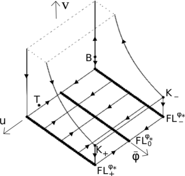
(a) The ski-slope state space with the six boundary sets in (31). Depicted are also solution trajectories on the $v=0$ subset with $\bar{\varphi}=\mathrm{constant}$, which are independent of the potential, as are the solution trajectories on the $u=\pm\sqrt{2}$ boundaries.

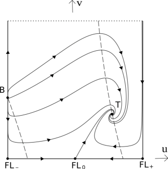
(b) The solution space structure on the $\bar{\varphi}=0$ boundary, where there are no bifurcations as $b>0$ and $p>0$ change. The dashed curves show where $v^{\prime}=0$; $v$ is increasing (decreasing) between (outside) the two $v^{\prime}=0$ curves. On this boundary the fixed point $\mathrm{B}$ is a source while $\mathrm{T}$ is a sink.

Figure 1: The ski-slope state space and the $\bar{\varphi}=0$ boundary. The dotted lines correspond to a cut off in $v$ in order to obtain a finite figure, since $v\rightarrow\infty$ when $\bar{\varphi}\rightarrow 0$, which also results in a cut off for small $\bar{\varphi}$ on the scalar field dominant boundary $v\bar{\varphi}=1/\sqrt{3}$.

Since the scalar field potential is not exponential, the scalar field contributes a source that is not scale-invariant. From this it follows that the Hubble scalar $H$ is a function of the state vector $(\bar{\varphi},u,v)$. By using (4c) in conjunction with (14) and (22) we obtain

$$3H^{2}=\frac{V}{\Omega_{V}}=\frac{2V}{(1-w_{\varphi})\Omega_{\varphi}}=\frac{2V(\bar{\varphi})}{3(2-u^{2})v^{2}\bar{\varphi}^{2}},$$ (32)

where

$$(3H^{2})^{\prime}=-2(1+q)(3H^{2})=-3(1+w_{\varphi}\Omega_{\varphi})(3H^{2})=-3[1+3(u^{2}-1)v^{2}\bar{\varphi}^{2}](3H^{2}),$$ (33)

as follows from the definitions of the new variables and (11). In the interior state space, where $\Omega_{\varphi}<1$ and $-1\leq w_{\varphi}<1$, it follows that $1+q>0$ and hence that $3H^{2}(u,v,\bar{\varphi})$ is monotonically decreasing. Thus, there are no periodic orbits (i.e. solution trajectories) or fixed points in the interior state space and hence all fixed points of the dynamical system (23) lie on the boundary of the ski-slope state space, given by (31) (in addition, an asymptotic analysis shows that there are no interior orbits that end at $\bar{\varphi}=0$ and $v=+\infty$).

3.3 Fixed points of the dynamical system

Some of the fixed points of the dynamical system (23) depend on $\lambda$ and thereby on the positive potential. Although not necessary, apart from the asymptotic condition (17a) we, for simplicity, assume that the potentials also satisfy the second condition (17b) and that the potentials are

• monotonically decreasing, i.e. $V_{,\varphi}<0$ and hence $\lambda(\varphi)>0$, or

• have a single positive minimum, i.e. there exists a positive finite $\varphi=\varphi_{0}$ such that $V_{,\varphi}|_{\varphi=\varphi_{0}}=0$ and $V_{,\varphi\varphi}|_{\varphi=\varphi_{0}}>0$ and hence $\lambda(\varphi_{0})=0$, $\lambda_{,\varphi}|_{\varphi=\varphi_{0}}<0$.

The matter dominant boundary $v=0$

It follows from (23) that the boundary set $v=0$ is independent of $\lambda$ and thereby also on the potential and that $v=0$ contains three Friedmann-Lemaître lines of fixed points:

$$\mathrm{FL}_{0}^{\varphi_{*}} \!: \qquad(\bar{\varphi},u,v) =(\bar{\varphi}_{*},0,0),$$ (34a)

$$\mathrm{FL}_{\pm}^{\varphi_{*}} \!: \qquad(\bar{\varphi},u,v) =(\bar{\varphi}_{*},\pm\sqrt{2},0),$$ (34b)

where the constant $\bar{\varphi}_{*}$ satisfies $0\leq\bar{\varphi}_{*}\leq 1$. Note that $w_{\varphi}=-1$ on $\mathrm{FL}_{0}^{\varphi_{*}}$ while $w_{\varphi}=1$ on $\mathrm{FL}_{\pm}^{\varphi_{*}}$. These fixed points correspond to the fixed points with the same labels in AUW [13] (see equations (24)). The lines of fixed points are connected by heteroclinic orbits (a heteroclinic orbit is a solution trajectory that connects two different fixed points) $\mathrm{FL}_{\pm}^{\varphi_{*}}\rightarrow\mathrm{FL}_{0}^{\varphi_{*}}$ that are straight lines with ‘frozen’ scalar field values $\bar{\varphi}=\bar{\varphi}_{*}=\mathrm{constant}$. The orbit structure on the boundary $v=0$ is shown in Figure 1(a).

The matter dominant boundary $\bar{\varphi}=0$

The boundary set $\bar{\varphi}=0$ reflects the unboundedness of $\lambda$, and this gives rise to new fixed points with $v>0$, as follows from (23):

$$\mathrm{T}:\quad(\bar{\varphi},u,v) =u_{\mathrm{T}}\left(0,1,\frac{1}{pb}\right),\qquad u_{\mathrm{T}}=\sqrt{\frac{p}{2+p}},$$ (35a)

$$\mathrm{B}:\quad(\bar{\varphi},u,v) =\sqrt{2}\left(0,-1,\frac{1}{4b}\right),$$ (35b)

where $b=F(0)>0$ is the constant defined in (19). On the boundary set $\bar{\varphi}=0$, a local analysis shows that the fixed point $\mathrm{T}$ is a spiral sink, $\mathrm{B}$ is a source (although $\mathrm{B}$ is a saddle in the full state space) and the three FL fixed points with $v=0$ are saddles. We conjecture that all interior orbits in the boundary set $\bar{\varphi}=0$ are attracted to $\mathrm{T}$. Although the details of the orbit structure on $\bar{\varphi}=0$ depend on the parameters $p$ and $b$, there are no bifurcations as the parameters change and thus the qualitative orbit structure on $\bar{\varphi}=0$ is independent of the potential; a representative description is shown in Figure 1(b) using the values $b=1$ and $p=3$.

The exponential boundary $\bar{\varphi}=1$

We have already noted that this boundary set coincides with the boundary set $\bar{\varphi}=1$ in AUW [13]. We briefly summarize the fixed points: apart from the $\bar{\varphi}=1$ boundary end points of the matter-dominated FL lines of fixed points with $v=0$ there are additional fixed points on the exponential $\bar{\varphi}=1$ boundary: the scalar field dominated ‘kinaton’ fixed points $\mathrm{K}_{\pm}$, the de Sitter fixed point $\mathrm{dS}$ (when $\lambda_{+}=0$), the power-law fixed point $\mathrm{P}$ (when $0<|\lambda_{+}|<\sqrt{6}$), and the scaling fixed point $\mathrm{S}$ (when $|\lambda_{+}|>\sqrt{3}$). The values of $u$ and $v$ for the fixed points on the $\bar{\varphi}=1$ boundary are:

$$\mathrm{K}_{\pm}\!:\quad(u,v) =\left(\pm\sqrt{2},{\textstyle{1\over\sqrt{3}}}\right),$$ (36a)

$$\mathrm{dS}:\quad(u,v) =\left(0,{\textstyle{1\over\sqrt{3}}}\right),\qquad\,\,\lambda_{+}=0,$$ (36b)

$$\mathrm{P}\!:\quad(u,v) ={\textstyle{1\over\sqrt{3}}}(\lambda_{+},1),\qquad 0<|\lambda_{+}|<\sqrt{6},$$ (36c)

$$\mathrm{S}\!:\quad(u,v) =\left(\text{sgn}(\lambda_{+}),{\textstyle{1\over|\lambda_{+}|}}\right),\qquad|\lambda_{+}|>\sqrt{3}.$$ (36d)

Details and figures depicting the orbit structures for the different cases associated with $\lambda_{+}=0$, $0<|\lambda_{+}|<\sqrt{3}$, $\sqrt{3}<|\lambda_{+}|<\sqrt{6}$, $\sqrt{6}<|\lambda_{+}|$ on the exponential boundary $\bar{\varphi}=1$ are given in AUW [13] while global results were proven in [17]. For monotonically decreasing potentials $\mathrm{P}$ is a sink (as is $\mathrm{dS}$ with $q=-1$ when $\lambda_{+}=0$); since $q=-1+\lambda_{+}^{2}/2$ at $\mathrm{P}$ it follows that $\lambda_{+}<\sqrt{2}$ results in future eternal acceleration, which we, for simplicity, henceforth assume when the potential is monotonically decreasing.

The scalar field dominant boundary $v\bar{\varphi}=1/\sqrt{3}$

For monotonically decreasing scalar field potentials with $\lambda(\varphi)>0$ and $0\leq\lambda_{+}<\sqrt{2}$, the function $3H^{2}$ in (33) is also a monotonic function on the interior of this boundary, although the evolution of $3H^{2}$ goes through an inflection point for orbits when and if they pass through $u=0$, which they only can do once since $u^{\prime}|_{u=0}>0$, and hence there are no periodic orbits or fixed points in the interior of the scalar field dominant boundary in this case.

Let us now turn to the case of a scalar field potential with a positive minimum. Apart from the previous fixed points, the minimum results in an additional fixed point given by

$$\mathrm{dS}^{0}\!:\quad(\bar{\varphi},u,v)=\left(\bar{\varphi}_{0},0,{\textstyle{1\over\sqrt{3}\,\bar{\varphi}_{0}}}\right),$$ (37)

where $\lambda(\bar{\varphi}_{0})=0$, $\bar{\varphi}_{0}\in(0,1)$, at the minimum of the potential. Since $\lambda_{,\varphi}|_{\bar{\varphi}=\bar{\varphi}_{0}}=-(V_{,\varphi\varphi}/V)|_{\bar{\varphi}=\bar{\varphi}_{0}}$ it follows that $\lambda_{,\varphi}|_{\bar{\varphi}=\bar{\varphi}_{0}}<0$ yields a positive minimum of the potential, and when this is the case, which we assume, the eigenvalues associated with $\mathrm{dS}^{0}$ have negative real parts and therefore $\mathrm{dS}^{0}$ is then a sink, which is a spiral on the scalar field dominant boundary if $\lambda_{,\varphi}|_{\bar{\varphi}=\bar{\varphi}_{0}}<-3/4$. When $-\sqrt{6}<\lambda_{+}<0$ the fixed point $\mathrm{P}$ exists, with one orbit originating from it ($\mathrm{P}$ is replaced with $\mathrm{dS}$ if $\lambda_{+}=0$) on the scalar field dominant boundary, but this fixed point leaves the state space when $\lambda_{+}=-\sqrt{6}$, which results in that all orbits on the scalar field dominant boundary (apart from the fixed point $\mathrm{dS}^{0}$) originate from an asymptotic cycle of boundary orbits and the limit $v\rightarrow+\infty$ where $u$ is monotonically increasing when $\lambda_{+}\leq-\sqrt{6}$, see Figure 2.

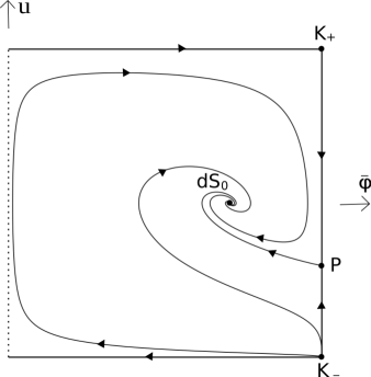
(a) $-\sqrt{6}<\lambda_{+}<0$

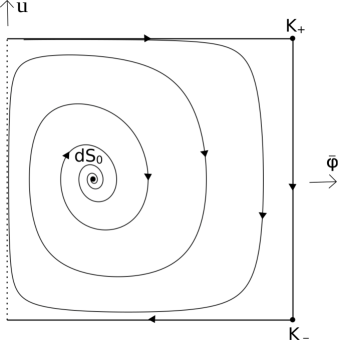
(b) $\lambda_{+}\leq-\sqrt{6}$

Figure 2: The orbit structure on the scalar field dominant boundary $v\bar{\varphi}=1/\sqrt{3}$ projected onto $(\bar{\varphi},u)$ with $0<\bar{\varphi}\leq 1$ on the horizontal axis and $u\in[-\sqrt{2},\sqrt{2}]$ on the vertical axis for the cases $-\sqrt{6}<\lambda_{+}<0$ and $\lambda_{+}\leq-\sqrt{6}$, respectively. These two cases are illustrated by the models given in eq. (39) with $p=1/2$, $\nu=2$ and the two values $\alpha=-1$ and $\alpha=-10$, which result in $\lambda_{+}=-1$ and $\lambda_{+}=-10$, respectively, since $\lambda_{+}=p\nu\alpha$ for these models. The dotted line corresponds to the cut off in $\bar{\varphi}$ on the scalar field dominant boundary in Figure 1.

We conclude this section by first summarizing the values of $\Omega_{\varphi}$ and $w_{\varphi}$ at the fixed points:

$$\Omega_{\varphi} =1\!:\qquad\mathrm{P},\,\mathrm{dS},\,\mathrm{dS}^{0},\,\mathrm{K}_{\pm}\qquad \text{with}\qquad w_{\varphi} ={\textstyle{\lambda_{+}^{2}\over 3}}-1,-1,-1,1,$$ (38a)

$$\Omega_{\varphi} =0\!:\qquad\mathrm{FL}_{0}^{\varphi_{*}},\,\mathrm{FL}_{\pm}^{\varphi_{*}},\,\mathrm{T},\,\mathrm{B}\qquad \text{with}\qquad w_{\varphi} =-1,1,-{\textstyle{2\over 2+p}},1,$$ (38b)

$$\Omega_{\varphi} ={\textstyle{3\over\lambda_{+}^{2}}}\!:\qquad\mathrm{S}\qquad \text{with}\qquad w_{\varphi} =0.$$ (38c)

As follows from (11), the deceleration parameter is given by $q=(1+3w_{\varphi}\Omega_{\varphi})/2$ and can be read off from the above values.

Finally, we notice that for the class of potentials under consideration the behaviour at late times of future accelerating models ($q<0$) is of three possible types:

• Monotonically decreasing potentials: if $0<\lambda_{+}<\sqrt{2}$ then the fixed point $\mathrm{P}$ is the sink, with $w_{\varphi}={\textstyle{\lambda_{+}^{2}\over 3}}-1$ and $q={\textstyle{\lambda_{+}^{2}\over 2}}-1$.

• Monotonically decreasing potentials: if $\lambda_{+}=0$ then the fixed point $\mathrm{dS}$ is the sink, with $w_{\varphi}=-1$ and $q=-1$.

• Potentials with a positive minimum: the fixed point $\mathrm{dS}^{0}$ is the sink, with $w_{\varphi}=-1$ and $q=-1$.

We conjecture, supported by heuristical arguments and numerical experiments, that in each case the sink is the future global attractor, denoted by ${\cal A}$, which thereby attracts all interior orbits, including those relevant for quintessence.

4 Quintessence

In this section we use the new dynamical system to describe and compare thawing, scaling freezing and tracking quintessence.

4.1 Observationally viable quintessence models

The first step is to identify which orbits in the ski-slope state space $(\bar{\varphi},u,v)$ that describe observationally viable quintessence models. We begin with two necessary conditions:

• The model must be accelerating at present and late times, i.e. $q<0,$ where $q$ is given by (11).

• The model must have an early long matter-dominated epoch ($\Omega_{\varphi}\lesssim 0.03$ for $\Delta N\sim 10$, see AUW [17]) and satisfy $\Omega_{\varphi}\approx 0.68$ at the present time $N=0$.

First we identify the orbits in the state space that begin at matter-dominated fixed points and then end at the future attractor ${\cal A}$. Then we regard these unstable manifolds as reference orbits in the sense that initial data sufficiently close to a fixed point of a viable reference orbit also provide viable quintessence models. Referring to (38) we see that the relevant fixed points are $\mathrm{FL}_{0}^{\varphi_{*}}$ with $0<\bar{\varphi}_{*}<1$, $\mathrm{T}$, and also $\mathrm{S}$ if the potential has a positive minimum and $\lambda_{+}\ll-1$. For a given potential belonging to the present class of potentials with unbounded $\lambda(\varphi)$ there are thereby three possibilities for reference orbits for generating viable quintessence models, which we denote symbolically as follows:

• a one parameter family of reference orbits $\mathrm{FL}_{0}^{\varphi_{*}}\rightarrow{\cal A}$ with $0<\bar{\varphi}_{*}<1$,

• a single reference orbit $\mathrm{S}\rightarrow{\cal A}=\mathrm{dS}^{0}$ when $\lambda_{+}\ll-1$,

• a single reference orbit $\mathrm{T}\rightarrow{\cal A}$,

where the future attractor ${\cal A}$ for monotonically decreasing potentials is given by $\mathrm{dS}$, $\mathrm{P}$ when $\lambda_{+}=0$, $0<\lambda_{+}<\sqrt{2}$, respectively, while ${\cal A}=\mathrm{dS}^{0}$ when the potential has a positive minimum. The reference orbits in all three cases are the unstable manifolds of the fixed points from which they originate. As we will see, the three sets of fixed points $\mathrm{FL}_{0}^{\varphi_{*}}$, $\mathrm{S}$ and $\mathrm{T}$ have stable manifolds that push nearby orbits (corresponding to open sets of initial data near the fixed points) to the unstable manifold orbits which they subsequently shadow until they all end at the future attractor ${\cal A}$. Next we discuss the three cases, which correspond to thawing, scaling freezing and tracking quintessence, respectively, in more detail.

Thawing quintessence

In case i) each fixed point of $\mathrm{FL}^{\varphi^{*}}_{0}$ has one eigenvalue that is zero (corresponding to the line of fixed points), one that is positive, which yields one reference orbit $\mathrm{FL}_{0}^{\varphi_{*}}\rightarrow{\cal A}$ for each fixed point of $\mathrm{FL}_{0}^{\varphi_{*}}$ (the unstable manifold of $\mathrm{FL}_{0}^{\varphi_{*}}$), and one negative eigenvalue corresponding to the stable manifold $v=0$ of $\mathrm{FL}^{\varphi^{*}}_{0}$ on which $\bar{\varphi}$ is constant/‘frozen’, shown in Figure 1. The condition of a long matter-dominated epoch is very restrictive and leads to initial data with $0<v\ll 1$, which result in open sets of orbits that are attracted/pushed toward to the unstable manifold reference orbits of $\mathrm{FL}^{\varphi^{*}}_{0}$, which they subsequently very closely shadow, until they all end at the future attractor ${\cal A}$. Note further that the equation of state for the reference orbits starts at $w_{\varphi}\approx-1$ ($w_{\varphi}=-1$ at $\mathrm{FL}^{\varphi^{*}}_{0}$) and then increases, which identify the reference orbits (and the orbits that shadow them) as thawing quintessence solutions. We discussed and elaborated on this type of quintessence in a dynamical systems setting for potentials with bounded ${\lambda}$ in AUW [13] and notice that the situation for thawing quintessence is quite similar in the present case with unbounded $\lambda$.

Scaling freezing quintessence

Case ii) occurs for a potential with a positive minimum. A matter-dominated scaling epoch for such potentials, where $\rho_{\varphi}$ approximately scales in time as $\rho_{\mathrm{m}}$, only holds for an open set of interior initial data sufficiently close to the fixed point $\mathrm{S}$. Moreover, since matter-dominance requires $\Omega_{\varphi}\lesssim 0.03\Rightarrow v\lesssim 0.1$ and since $v|_{\mathrm{S}}=1/|\lambda_{+}|$ it follows that matter-dominated scaling orbits require $\lambda_{+}\lesssim-10$. The fixed point $\mathrm{S}$ has two negative eigenvalues with the boundary $\bar{\varphi}=1$ as the stable manifold on which $\mathrm{S}$ attracts all orbits, and one positive eigenvalue, which makes $\mathrm{S}$ a saddle point in the full state space, where the reference orbit $\mathrm{S}\rightarrow\mathrm{dS}^{0}$ is the unstable manifold associated with the positive eigenvalue. The open set of interior matter-dominated scaling initial data sufficiently close to $\mathrm{S}$ first approach $\mathrm{S}$ and then the reference orbit, which they then shadow, and then they all finally end at $\mathrm{dS}^{0}$. Due to that these orbits, and the reference orbit, exhibit the scaling property during the matter-dominated epoch near $\mathrm{S}$ where $w_{\varphi}\approx w_{\mathrm{m}}=0$, and since $w_{\varphi}=-1$ at $\mathrm{dS}^{0}$, these orbits correspond to scaling freezing quintessence solutions, see e.g. Tsujikawa (2013) [4].

Tracking quintessence

In this paper we focus on case iii). The fixed point $\mathrm{T}$ has two eigenvalues with negative real parts with the matter dominant boundary $\bar{\varphi}=0$ as its stable manifold on which $\mathrm{T}$ attracts all orbits and one positive eigenvalue, making $\mathrm{T}$ a saddle point in the full state space where the positive eigenvalue yields the unstable manifold reference orbit $\mathrm{T}\rightarrow{\cal A}$.

Since, according to (30), $\Delta=\bar{\varphi}\lambda(\bar{\varphi})\,v/u=G(\bar{\varphi})v/u$ where $G(0)=p\,b$, $u_{\mathrm{T}}=p\,b\,v_{\mathrm{T}}$, it follows that $\Delta=1$ at the fixed point $\mathrm{T}$, i.e. the first tracker condition is exactly fulfilled at $\mathrm{T}$. Since we can write $\lambda=(p/\varphi)f(\varphi)$, where $f$ is regular and satisfies $f(0)=1$ due to the boundedness condition (17a) and since $\Gamma=1-\lambda_{,\varphi}/\lambda^{2}$ it follows that $\Gamma-1=1/p>1$ when $\varphi\rightarrow 0$ and hence at $\mathrm{T}$, while $w_{\varphi}|_{\mathrm{T}}=u_{\mathrm{T}}^{2}-1=-2/(2+p)<0$ and thus the second tracker condition is also fulfilled at $\mathrm{T}$. We therefore refer to $\mathrm{T}$ as the tracker fixed point and the unstable manifold reference orbit of $\mathrm{T}$ as the tracker orbit. When $w_{\varphi}(N)$ is nearly constant, which is true near $\mathrm{T}$, the graph of $w_{\varphi}(N)$ has a horizontal plateau $w_{\varphi}\approx-2/(2+p)$, as illustrated in the graphs of $w_{\varphi}(N)$ in section 5.

If $\bar{\varphi}$ is sufficiently close to the matter dominant boundary $\bar{\varphi}=0$ this results in an open set of initial conditions that yields orbits with a long matter-dominated epoch where they a) shadow the orbits on $\bar{\varphi}=0$, see Figure 1(b), b) then approach and spiral around $\mathrm{T}$, where they still are matter-dominated but where being close to $\mathrm{T}$ also implies that the orbits approximately obey the tracker conditions, c) and where they subsequently track/shadow the tracker orbit until they all end at the future attractor ${\cal A}$. Steinhardt et al. (1999) [7] characterizes the open set of orbits that track/shadow the tracker orbit as undershooting and overshooting orbits. In terms of our state space description this characterization is based on solutions with initial data close to $\bar{\varphi}=0$ with $u\lesssim 0$, $0\lesssim v<v_{\mathrm{T}}$ (undershooting solutions), and $u\gtrsim 0$, $v\gg v_{\mathrm{T}}$ (overshooting solutions). We will give specific examples in section 5.

In this way, to quote Steinhardt et al. (1999) [7] (see the introduction), who dealt with monotonically decreasing potentials for which $\lambda_{+}=0$, primarily the inverse power-law potential: ”…a very wide range of initial conditions rapidly converge to a common, cosmic evolutionary track.” However, it is worth noticing that for monotonically decreasing potentials with ${\cal A}=\mathrm{dS}$ the fixed point $\mathrm{dS}$ has an eigenvalue that is zero with a stable interior state space center manifold direction, and two eigenvalues with negative real parts with the boundary $\bar{\varphi}=1$ as their associated stable manifold. As a consequence all orbits are strongly attracted to the center manifold of $\mathrm{dS}$, which means that they all ‘track’ each other, including tracking/shadowing the tracker orbit.

Finally, we comment on the dynamical systems approach by Bahamonde et al. (2018) used in [5] to study tracking quintessence for the inverse power-law potential. To do so they introduced variables that result in a non-regular system that breaks down when $\varphi\rightarrow 0$ (when their variable $z$ is one, see their eqs. 4.37-4.38). They then regularize their equations by changing the time variable to obtain the system 4.40-4.42. However, this hides that the new time variable asymptotically breaks down when $\varphi\rightarrow 0$ and that their variables deform and crush our regular dynamical system at $\bar{\varphi}=0$. This results in half circles at $z=1$ and a fixed point at the intersection of two lines of fixed points at $x=0$ on the line of fixed points $B_{x}$, see Figure 9 in [5]. The eigenvalues at this fixed point are all zero, see Table 7 in [5]. The authors then perform a numerical investigation that suggests that the tracker orbit originates from the fixed point $x=0$ on $B_{x}$.

In contrast to our regularized dynamical system with a time variable that does not break down when $\varphi\rightarrow 0$, the variables and dynamical system 4.40-4.42 in [5] cannot be used to: 1) explain the tracking attractor feature, which our variables show is due to that $\bar{\varphi}=0$ is the stable manifold of $\mathrm{T}$, 2) nor can the dynamical system 4.40-4.42 be used to obtain analytic approximations for the tracker orbit since all eigenvalues are zero at $x=0$ on $B_{x}$, while we will use the unstable manifold corresponding to the positive eigenvalue at $\mathrm{T}$ to obtain simple and accurate approximations for tracker orbits for a wide range of potentials in a future follow up paper.

4.2 Thawing, scaling freezing and tracking quintessence

We conclude this section with some further comments on thawing, scaling freezing and tracking quintessence for a potential with unbounded $\lambda$. We first note that there is a close mathematical relationship between the present models with unbounded $\lambda(\varphi)$ and tracking quintessence and models with bounded $\lambda(\varphi)$ that have a very large $\lambda_{-}$ and thereby admit scaling quintessence associated with $\varphi\rightarrow-\infty$. The two cases have a fixed point $\mathrm{T}$ and $\mathrm{S}$, respectively, with stable manifolds on a boundary associated with their respective scalar field limits, and both have a single reference orbit as their unstable manifold that attracts an open set of orbits that come close to the fixed point; cf. AUW [13] with the present paper, especially the illustrative figures in AUW and in the next section. However, recall that $\Omega_{\varphi}=3/\lambda_{+}^{2}$, $1\ll|\lambda_{+}|$ and hence $0<\Omega_{\varphi}\ll 1$ at $\mathrm{S}$ for scaling freezing quintessence while $\Omega_{\varphi}=0$ for tracking (and thawing) quintessence at $\mathrm{T}$ (and $\mathrm{FL}^{\varphi_{*}}$).

We finally comment on the distinction between tracking, scaling freezing and thawing quintessence, which is not as clear cut as it first appears. We first note that scalar field potentials always give rise to an open set of thawing quintessence solutions (where some of the thawing solutions are observationally compatible with the $\Lambda$CDM model if a scalar field potential has a sufficiently slowly changing part) shadowing the thawing quintessence reference orbits. If the present class of potentials exhibits a positive minimum and $\lambda_{+}\ll-1$ then apart from the open sets of orbits that exhibit thawing and tracking quintessence there also exists an open set of scaling freezing quintessence orbits. The coexistence of thawing quintessence with tracking and also scaling freezing quintessence (if the potential has a minimum and $\lambda_{+}\ll-1$) causes complications as regards distinguishing thawing quintessence from tracking and scaling freezing quintessence. This complication is caused by the orbits $\mathrm{FL}_{0}\rightarrow\mathrm{T}$ and $\mathrm{FL}_{0}\rightarrow\mathrm{S}$ in the boundary sets $\bar{\varphi}=0$ and $\bar{\varphi}=1$, respectively. It follows that the unstable manifold of any fixed point $\mathrm{FL}_{0}^{\varphi_{*}}$ with $0<\bar{\varphi}_{*}\ll 1$ ($0\ll\bar{\varphi}_{*}<1$) will shadow the orbit $\mathrm{FL}_{0}\rightarrow\mathrm{T}$ ($\mathrm{FL}_{0}\rightarrow\mathrm{S}$) and hence pass close to $\mathrm{T}$ ($\mathrm{S}$), giving rise to solutions that are both thawing and tracking (scaling freezing) quintessence models. To avoid this ambiguity we impose the restriction $0\ll\bar{\varphi}_{*}<1$ (and $0\ll\bar{\varphi}_{*}\ll 1$ for potentials with a minimum and $\lambda_{+}\ll-1$) when describing thawing quintessence models.

5 Numerical simulations for tracking quintessence

Instead of using the inverse power-law potential as an illustrative example, we use the following more versatile class of hyperbolic potentials:

$$V=V_{0}\left[\frac{\nu(\cosh\nu\varphi)^{1-\alpha}}{\sinh(\nu\varphi)}\right]^{p}\quad\implies\quad\lambda=\frac{p\nu}{\tanh{\nu\varphi}}\left[1+(\alpha-1)(\tanh{\nu\varphi})^{2}\right],$$ (39)

where $\varphi\in(0,\infty)$, $p>0$, $\nu>0$, while $\alpha$ is arbitrary, and

$$\lambda_{+}=p\nu\alpha.$$ (40)

For these models a suitable choice of $\bar{\varphi}$ is

$$\bar{\varphi}=\tanh(\nu\varphi)\quad\implies\quad F(\bar{\varphi})=\nu(1-\bar{\varphi}^{2}),$$ (41)

satisfying (19) with $b=\nu$, which leads to

$$G(\bar{\varphi})=p\nu\left[1+(\alpha-1)\bar{\varphi}^{2}\right],\qquad\Gamma-1=\frac{(1-\bar{\varphi}^{2})(1-(\alpha-1)\bar{\varphi}^{2})}{p[1+(\alpha-1)\bar{\varphi}^{2}]^{2}},$$ (42)

where $\Gamma>1$ globally if $\alpha<2$. The special cases $\alpha=1$ and $\alpha=0$ with $V\propto\sinh^{-p}(\nu\varphi)$ and $V\propto\tanh^{-p}(\nu\varphi)$, respectively, are well known.

We note that if we use the illustrative positive potential (39) a minimum of such a potential implies that $\alpha<0$ and where the fixed point $\mathrm{dS}^{0}$ is located at $\bar{\varphi}_{0}=1/\sqrt{1-\alpha}$. In order for $\mathrm{dS}^{0}$ not only to be a sink but a spiral sink it follows that $p\nu^{2}\alpha<-3/8$, which follows from the spiral condition $\lambda_{,\varphi}|_{\bar{\varphi}=\bar{\varphi}_{0}}<-3/4$ in footnote 11 where $\lambda_{,\varphi}|_{\bar{\varphi}=\bar{\varphi}_{0}}=2p\nu^{2}\alpha$ for the present models. We will use these models to illustrate that there are three types of tracker orbits for potentials that are monotonically decreasing: those for which $w_{\varphi}$ is overall decreasing, constant, and increasing, and then we will turn to the case of a potential with a positive minimum.

5.1 Monotonic potentials: Three types of tracker orbits

The central features for tracking quintessence are the tracker fixed point $\mathrm{T}$ and the tracker orbit $\mathrm{T}\rightarrow{\cal A}$, where ${\cal A}$ is one of the fixed points $\mathrm{P}$, $\mathrm{dS}$ for monotonically decreasing potentials depending on whether $0<\lambda_{+}<\sqrt{2}$ or $\lambda_{+}=0$, respectively. We then note that

$$1+w_{\varphi}|_{\mathrm{T}}=u_{\mathrm{T}}^{2}=\frac{p}{2+p},\qquad 1+w_{\varphi}|_{\mathrm{P}/\mathrm{dS}}=u_{\mathrm{P}/\mathrm{dS}}^{2}=\frac{1}{3}\lambda_{+}^{2}=\frac{1}{3}(p\nu\alpha)^{2},$$ (43)

where the last equality follows from (40). Hence the overall decrease/increase of $w_{\varphi}$ for the tracker orbit $\mathrm{T}\rightarrow{\cal A}$ is determined by the values of $u_{\mathrm{T}}$ and $u_{\mathrm{P}}$ (or, possibly, $u_{\mathrm{dS}}$ when $w_{\varphi}$ is overall decreasing), which leads to:

$$\sqrt{3}u_{\mathrm{T}} =\sqrt{\frac{3p}{2+p}}>\sqrt{3}u_{\mathrm{P}/\mathrm{dS}}=\lambda_{+}, \text{overall decrease in $w_{\varphi}$},$$ (44a)

$$\sqrt{3}u_{\mathrm{T}} =\sqrt{\frac{3p}{2+p}}=\sqrt{3}u_{\mathrm{P}}=\lambda_{+}, \text{overall constant $w_{\varphi}$},$$ (44b)

$$\sqrt{3}u_{\mathrm{T}} =\sqrt{\frac{3p}{2+p}}<\sqrt{3}u_{\mathrm{P}}=\lambda_{+}, \text{overall increase in $w_{\varphi}$},$$ (44c)

where we recall that $\lambda_{+}=p\nu\alpha$ for the potentials (39).

It does not follow in general that $w_{\varphi}$ is constant during the evolution for the borderline case (44b), although there is no overall change in $w_{\varphi}$ during the evolution from $\mathrm{T}$ to $\mathrm{P}$. However, suitable restrictions on the parameters $\alpha$, $p$, $\nu$ for the potentials (39) give rise to a subclass of potentials for which $w_{\varphi}=u^{2}-1$ is constant for a particular solution. In the early years of quintessence, Sahni and Starobinsky (2000) [21], equation (121), and Urena-Lopez and Matos (2000) [19], investigated models with the potential (39) with $\alpha=1$, i.e. $V\propto\sinh^{-p}(\nu\varphi)$, and pointed out that these models admitted a special solution for which $w_{\varphi}$ is constant. This model corresponds to the tracker orbit when $w_{\varphi}|_{\mathrm{T}}=w_{\varphi}|_{\mathrm{P}}$ and hence $\sqrt{3}u_{\mathrm{T}}=\sqrt{3}u_{\mathrm{P}}=\lambda_{+}=p\nu$, where the last equality follows from setting $\alpha=1$ in (40), which results in $\sqrt{3p/(2+p)}=p\nu$, and hence

$$\nu=\sqrt{\frac{3}{p(2+p)}}.$$ (45)

Positive potentials $V\propto\sinh^{-p}(\nu\varphi)$ with any value of $p>0$ and the above value of $\nu$ result in that the tracker orbit $\mathrm{T}\rightarrow\mathrm{P}$ is a straight line in the state space $(\bar{\varphi},u,v)$, parallel to the $\bar{\varphi}$ axis given by $u=u_{\mathrm{T}}=\sqrt{p/(2+p)}$, $v=v_{\mathrm{T}}=u_{\mathrm{T}}/p\nu=1/\sqrt{3}$, and thereby with a constant $w_{\varphi}$ given by $1+w_{\varphi}=u_{\mathrm{T}}^{2}=p/(2+p)$. Furthermore, since $\Omega_{\varphi}=3v^{2}\bar{\varphi}^{2}$ it follows that $\Omega_{\varphi}=\bar{\varphi}^{2}$.

Along any of the above three types of tracker orbits, the graph of $w_{\varphi}$ begins during matter-dominance ($\Omega_{\varphi}\approx 0$) close to $\mathrm{T}$ with a horizontal plateau $w_{\varphi}\approx-2/(2+p)$, i.e. $-1<w_{\varphi}<0$. During the evolution $\Omega_{\varphi}$ thereby starts close to zero near $\mathrm{T}$ and then increases to 1 at ${\cal A}$. The present epoch at $N=0$ is characterized by that $\Omega_{\varphi}(N)$ reaches the observed value $\Omega_{\varphi}(0)=\Omega_{\varphi,0}\approx 0.68$. The value of $w_{\varphi}$ at late times depends on ${\cal A}$ but its value at the present time depends on $\lambda(\bar{\varphi})$ at $\bar{\varphi}(N=0)$. For monotonically decreasing potentials with $\lambda_{+}=0$ the tracker orbit approaches $\mathrm{dS}$ and hence $w_{\varphi}\rightarrow-1$ asymptotically, but is greater than $-1$ when $N=0$. These features are illustrated in Figure 3.

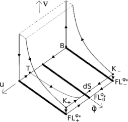
(a) Tracker orbit for the potential (39) with $\alpha=0$, and $\nu=p=3$.

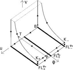
(b) Tracker orbit for the potential (39) with $\alpha=1$, $\nu=\sqrt{\frac{12}{5}}$ and $p=0.5$.

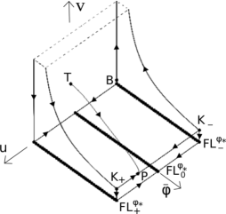
(c) Tracker orbit for the potential (39) with $\alpha=12$, $\nu=2$ and $p=0.05$.

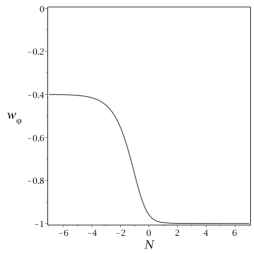
(d) Decreasing $w_{\varphi}(N)$ for the tracker orbit with a potential (39) with $\alpha=0$, and $\nu=p=3$.

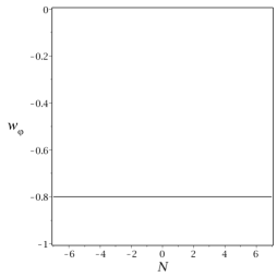
(e) Constant $w_{\varphi}(N)$ for the tracker orbit with a potential (39) with $\alpha=1$, $\nu=\sqrt{\frac{12}{5}}$ and $p=0.5$.

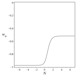
(f) Increasing $w_{\varphi}(N)$ for the tracker orbit with a potential (39) with $\alpha=12$, $\nu=2$ and $p=0.05$.

Figure 3: Tracker orbits in the ski-slope state-space and the respective graph of $w_{\varphi}(N)$ for the potential (39), illustrating that $w_{\varphi}$ can decrease, be a constant, and increase for the tracker orbit.

5.2 The tracker orbit for a potential with a minimum

In this case $\mathrm{T}\rightarrow\mathrm{dS}^{0}$ where the sink $\mathrm{dS}^{0}$ resides on the matter dominant boundary $v\bar{\varphi}=1/\sqrt{3}$ with $\bar{\varphi}=\bar{\varphi}_{0}$ determined by $\lambda(\bar{\varphi}_{0})=0$. If $\lambda_{,\varphi}|_{\bar{\varphi}=\bar{\varphi}_{0}}<-3/4$, then, according to footnote 11, $\mathrm{dS}^{0}$ is a spiral focus sink in the boundary set $v\bar{\varphi}=1/\sqrt{3}$ (see Figures 2 and 4). The fixed point $\mathrm{dS}^{0}$ has another feature which helps to describe how the orbits are attracted to $\mathrm{dS}^{0}$, including the tracker orbit. There is an orbit $\mathrm{FL}_{0}^{\varphi_{*}}\rightarrow\mathrm{dS}^{0}$ that is a straight line characterized by $\bar{\varphi}=\bar{\varphi}_{*}=\bar{\varphi}_{0}$, $u=0$, $0<v<1/\sqrt{3}$. This orbit describes the $\Lambda$CDM solution, which corresponds to that the scalar field resides in the positive minimum of the potential, where $\lambda(\bar{\varphi}_{0})=0=G(\bar{\varphi}_{0})$, giving rise to $\Lambda=V(\bar{\varphi}_{0})>0$. All interior orbits are asymptotic to the spiral (assuming that $\lambda_{,\varphi}|_{\bar{\varphi}=\bar{\varphi}_{0}}<-3/4$) sink $\mathrm{dS}^{0}$ and hence as they come close to $\mathrm{dS}^{0}$ they spiral around the $\Lambda$CDM orbit. In particular, the tracker orbit $\mathrm{T}\rightarrow\mathrm{dS}^{0}$ originates from ${\mathrm{T}}$ with $\Delta\approx 1$, $w_{\varphi}\approx\mathrm{constant}$ and then it bends and eventually forms a spiral around the $\Lambda$CDM orbit as it approaches $\mathrm{dS}^{0}$. These features are illustrated in Figure 4.

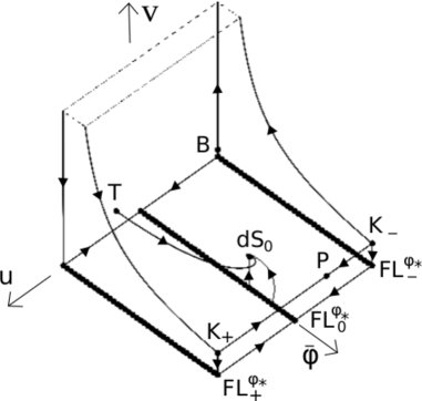
(a) Tracker, $\Lambda$CDM, and a thawing quintessence orbit for the potential (39) with $\nu=2$, $p=1/2$, and $\alpha=-1$.

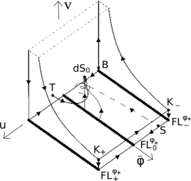
(b) Tracker, $\Lambda$CDM, scaling freezing, and a thawing quintessence orbit for the potential (39) with $\alpha=-10$, $\nu=2$ and $p=1/2$.

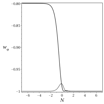
(c) Graphs of $w_{\varphi}$ for the tracker and thawing quintessence orbits for the potential (39) with $\nu=2$, $p=1/2$, and $\alpha=-1$.

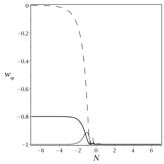
(d) Graphs of $w_{\varphi}$ for the tracker, thawing and scaling freezing quintessence orbits for the potential (39) with $\nu=2$, $p=1/2$, and $\alpha=-10$.

Figure 4: The tracker orbit in the ski-slope state-space and their graphs $w_{\varphi}(N)$ for the potential (39) with a minimum, together with the $\Lambda$CDM orbit, a thawing quintessence reference orbit originating from $\mathrm{FL}_{0}^{\varphi_{*}}$, and also a scaling freezing quintessence reference orbit when $\lambda_{+}\ll-1$ in figure (b), with associated graphs of $w_{\varphi}$ in (c) and (d), where $w_{\varphi}$ for the thawing orbit begins with $w_{\varphi}\approx-1$, while the tracker orbit begins with $w_{\varphi}\approx-2/(2+p)$, which for $p=1/2$ yields $w_{\varphi}\approx-0.8$, and where the dashed scaling freezing orbit begins with $w_{\varphi}\approx 0$.

5.3 Tracking quintessence for an open set of initial data

Recall that Steinhardt et al. (1999) [7] characterized the open set of orbits tracking/shadowing the tracker orbit as undershooting and overshooting orbits, which corresponds to $u\lesssim 0$, $0\lesssim v<v_{\mathrm{T}}$ (undershooting solutions) and $u\gtrsim 0$, $v\gg v_{\mathrm{T}}$ (overshooting solutions), where the condition of a long matter-dominated epoch requires these conditions for initial data to be supplemented by a very small value of $\bar{\varphi}$ near the $\bar{\varphi}=0$ matter dominant boundary. Solutions corresponding to such initial data shadow orbits on the $\bar{\varphi}=0$ boundary, where we can use Figure 1(b) to obtain a feeling for how the solutions behave before they begin to spiral around $\mathrm{T}$ in its vicinity during the matter-dominated epoch. Since $w_{\varphi}=u^{2}-1$ this also gives a feeling for how graphs of $w_{\varphi}$ behave, however, recall that the scalar field is essentially a test field during the matter-dominated epoch and hence that this behaviour of $w_{\varphi}$ is not an observable property and thereby physically unimportant. These features are illustrated in Figure 5. The graph $w_{\varphi}(N)$ in Figure 5(c) of the overshooting (dashed) orbit in Figures 5(a) and 5(b) covers the stage when it is very close to the boundary orbit at $\bar{\varphi}=0$, $u=\sqrt{2}$ where $w_{\varphi}=1$ (earlier it shadowed an orbit on the $\bar{\varphi}=0$ boundary that passed $u=0$ at a very large value of $v$ not shown), subsequently, due to that $\bar{\varphi}^{\prime}>0$, it shadows a nearby orbit on the $u=\sqrt{2}$ boundary, see Figure 5(b), which is followed by shadowing an orbit $\mathrm{FL}_{+}^{\varphi_{*}}\rightarrow\mathrm{FL}_{0}^{\varphi_{*}}$ with $\bar{\varphi}=\mathrm{constant}\ll 1$, and then an unstable $\mathrm{FL}_{0}^{\varphi_{*}}$ reference orbit near the orbit $\mathrm{FL}_{0}^{\varphi_{*}}\rightarrow\mathrm{T}$ on $\bar{\varphi}=0$, and finally it shadows the tracker orbit $\mathrm{T}\rightarrow\mathrm{dS}$; the graph $w_{\varphi}(N)$ in Figure 5(c) of the undershooting (dotted) orbit in Figures 5(a) and 5(b) covers the stage when this undershooting orbit shadows an orbit on the $\bar{\varphi}=0$ boundary when it passes $u=0$ where $w_{\varphi}=-1$ and afterwards where it, due to that $\bar{\varphi}^{\prime}<0$ when $u<0$, comes extremely close to $\mathrm{T}$ and where it subsequently shadows the tracker orbit $\mathrm{T}\rightarrow\mathrm{dS}$ (both the overshooting and undershooting orbits basically overlap with the tracker orbit after the matter-dominated tracker stage, where the tracker solution therefore describes the quintessence epoch of the overshooting and undershooting solutions extremely well).

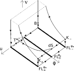
(a) Tracker, undershooting and overshooting orbits.

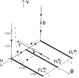
(b) Tracker, undershooting and overshooting orbits in the vicinity of $\bar{\varphi}=0$.

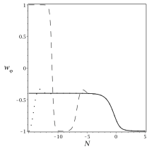
(c) Graphs of $w_{\varphi}(N)$ for the tracker, undershooting and overshooting solutions.

Figure 5: The tracker orbit (full line), overshooting (dashed line) and undershooting (dotted line) orbits in the ski-slope state-space and their graphs $w_{\varphi}(N)$ for the monotonically decreasing positive potential (39) with $\nu=1$, $p=3$ and $\alpha=0$.

6 Concluding remarks

We have given, for the first time, a description of tracking quintessence in a regular state space framework using the $e$-fold time $N$, showing that it is generated by any potential for which $\lambda$ is unbounded with $\varphi\lambda\rightarrow p>0$ as $\varphi\rightarrow 0$. A central role is played by a unique tracker orbit that originates from the tracker fixed point $\mathrm{T}$ which then governs the transition from matter-domination to quintessence-domination and an accelerating universe. Our state space provides some clarification for the claim of Steinhardt et al. (1999) [7] that with tracking quintessence, ”a very wide range of initial conditions rapidly converge to a common, cosmic evolutionary track of $\rho_{\varphi}(N)$ and $w_{\varphi}(N)$”.

We have shown that potentials with unbounded $\lambda$ also lead to thawing and scaling freezing quintessence (the latter for potentials with a positive minimum and $\lambda_{+}\ll-1$) and have used the state space to make a distinction between the three types, based on which fixed points the reference orbits originate from (cf. with the more complicated classification used in AUW[13]). One might ask: Which of the open sets of different types of quintessence initial data is preferred? Why should tracking quintessence have a special status?

Finally, we note that the present dynamical systems formulation can be slightly modified to obtain simple and accurate approximations with the $\Lambda$CDM model as a continuous parameter/initial data limit for tracking and thawing quintessence, which will be the topic of a forthcoming paper.

Acknowledgments

A. A. is supported by FCT/Portugal through CAMGSD, IST-ID, projects UIDB/04459/2020 and UIDP/04459/2020, and by the H2020-MSCA-2022-SE project EinsteinWaves, GA No. 101131233. A.A. would also like to thank the CMA-UBI in Covilhã for kind hospitality. C. U. would like to thank the CAMGSD, Instituto Superior Técnico in Lisbon for kind hospitality.

References

- [1] A. G. Riess et al. Observational evidence from supernovae for an accelerating universe and a cosmological constant. Astron. J., 116:1009, 1998.
- [2] S. Perlmutter et al. Measurements of omega and lambda from 42 high redshift supernovae. Astron. J., 517:565, 1999.
- [3] R. R. Caldwell, Rahul Dave, and Paul J. Steinhardt. Cosmological imprint of an energy component with general equation of state. Phys. Rev. Lett., 80:1582–1585, 1998.
- [4] S. Tsujikawa. Quintessence: a review. Class. Quantum Grav., 30:214003, 2013.
- [5] S. Bahamonde, C. G. Böhmer, S. Carloni, E. J. Copeland, Wei Fang, and N. Tamanini. Dynamical systems applied to cosmology: Dark energy and modified gravity. Physics Reports, 775-777:1–122, 2018.
- [6] I. Zlatev, L. Wang, and P. J. Steinhardt. Quintessence, cosmic coincidence and the cosmological constant. Phys. Rev. Lett., 82:896, 1999.
- [7] P. J. Steinhardt, L. Wang, and I. Zlatev. Cosmological tracking solutions. Phys. Rev. D, 59:123504, 1999.
- [8] P. J. E. Peebles and B. Ratra. Cosmology with a time variable cosmological constant. Astro. Phys. J., 325:L17, 1988.
- [9] B. Ratra and P. J. E. Peebles. Cosmological consequences of a rolling homogeneous scalar field. Phys. Rev. D, 37:3406, 1988.
- [10] B. Ratra and A. Quillen. Gravitational lensing effects in a time-variable cosmological ‘constant’ cosmology. Monthly Notices of the Royal Astronomical Society, 259(4):738–742, 12 1992.
- [11] S. Podariu and B. Ratra. Supernova ia constraints on a time-variable cosmological “constant”. The Astrophysical Journal, 532(1):109, mar 2000.
- [12] P. J. E. Peebles and Bharat Ratra. The cosmological constant and dark energy. Rev. Mod. Phys., 75:559–606, 2003.
- [13] A. Alho, C. Uggla, and J. Wainwright. Quintessence from a state space perspective. Physics of the Dark Universe, 39:101146, 2023.
- [14] A. Alho and C. Uggla. Quintessential -attractor inflation: A dynamical systems analysis. Journal of Cosmology and Astroparticle Physics, 11:083, 2023.
- [15] A. Alho and C. Uggla. Scalar field deformations of lambda-cdm cosmology. Phys. Rev. D, 92(10):103502, 2015.
- [16] C. Rubano, P. Scudellaro, and E. Piedipalumbo. Exponential potentials for tracker fields. Phys. Rev. D, 69:103510, 2004.
- [17] A. Alho, W. C. Lim, and C. Uggla. Cosmological global dynamical systems analysis. Class. Quantum Grav., 39:145010, 2022.
- [18] T. Chiba, A. De Felice, and S. Tsujikawa. Observational constraints on quintessence: Thawing, tracker and scaling models. Phys. Rev. D, 87:083505, 2013.
- [19] L.A. Urena-Lopez and T. Matos. New cosmological tracker solution for quintessence. Phys. Rev. D, 62:081302, 2000.
- [20] S. Bag, S.S. Mishra, and V. Sahni. New tracker models of dark energy. Journal of Cosmology and Astroparticle Physics, 08:009, 2018.
- [21] V. Sahni and A.Starobinsky. The case for a positive cosmological lambda-term. Int. J. Mod. Phys. D, 9:373, 2000.