Heat Pulses in Electron Quantum Optics

Abstract

Electron quantum optics aims to realize ideas from the quantum theory of light with the role of photons being played by charge pulses in electronic conductors. Experimentally, the charge pulses are excited by time-dependent voltages, however, one could also generate heat pulses by heating and cooling an electrode. Here, we explore this intriguing idea by formulating a Floquet scattering theory of heat pulses in mesoscopic conductors. The adiabatic emission of heat pulses leads to a heat current that in linear response is given by the thermal conductance quantum. However, we also find a high-frequency component, which ensures that the fluctuation-dissipation theorem for heat currents, whose validity has been debated, is fulfilled. The heat pulses are uncharged, and we probe their electron-hole content by evaluating the partition noise in the outputs of a quantum point contact. We also employ a Hong–Ou–Mandel setup to examine if the pulses bunch or antibunch. Finally, to generate an electric current, we use a Mach–Zehnder interferometer that breaks the electron-hole symmetry and thereby enables a thermoelectric effect. Our work paves the way for systematic investigations of heat pulses in mesoscopic conductors, and it may stimulate future experiments.

Introduction.— Electron quantum optics is an emerging field of mesoscopic physics in which charge pulses are emitted into electronic circuits to realize interference experiments with electrons [1, 2, 3]. Clean single-particle excitations can be generated by applying Lorentzian voltage pulses to an electrode [4, 5, 6, 7, 8], and the edge states of a quantum Hall sample can be shaped to form electronic circuits such as Mach–Zehnder [9] or Fabry–Pérot interferometers [10]. Charges that are emitted close to the Fermi level can often be treated as non-interacting, for example, when interfering at an electronic beam splitter [11, 7, 8]. By contrast, at high energies, recent collision experiments have revealed strong interactions and non-linear effects [12, 13, 14]. These advances show how experiments with time-dependent voltages bring about many exciting opportunities compared to their static counterparts.

Instead of generating charge pulses with a voltage, one could also excite heat pulses by heating and cooling an electrode to generate a time-dependent temperature [15, 16, 17]. The generation of heat pulses in electron quantum optics is largely unexplored, and it could open up for a wide range of future applications and fundamental investigations [18, 19, 20, 21, 22, 23]. For example, heat pulses should be electrically neutral, which might make them less prone to interaction and decoherence effects [24]. Fast control of energy is also becoming increasingly important for heat management at the nano-scale and for converting waste heat into useful work [25, 26]. Experiments with constant temperature biases have already observed the quantization of the thermal conductance in electronic conductors [27, 28, 29], while non-abelian states have been shown to exhibit fractional thermal conductance [30, 31]. By contrast, much less is known about the propagation of heat pulses in mesoscopic conductors.

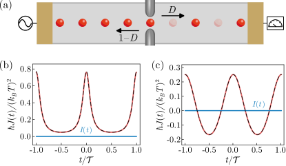
Figure 1: Periodic heat pulses in a mesoscopic conductor. (a) Two-terminal setup with a source and a drain electrode connected by a quantum point contact with transmission $D$. Heat pulses are emitted from the source electrode, and the electric current and the heat current are measured in the drain electrode. (b) Heat current for Lorentzian pulses of period $\mathcal{T}$, half-width $\Gamma=0.1\mathcal{T}$, and amplitude $W_{0}=0.3$. The base temperature is $k_{B}T=3\hbar\Omega$ with $\Omega=2\pi/\mathcal{T}$, and the quantum point contact is fully open, $D=1$. The dashed line indicates the static result in Eq. (5) with the time-dependent temperature of the source electrode inserted, $T_{S}=[1+W(t)]T$, where $W(t)$ is defined in Eq. (4). The electric current vanishes. (c) Similar results for a cosine drive with amplitude $W_{0}=0.4$.

In this Letter, we formulate a Floquet scattering theory of heat pulses in mesoscopic conductors. To this end, we perform work on an electrode, which causes its temperature to change and leads to the periodic emission of heat pulses, see Fig. 1(a). At low frequencies compared to the base temperature, the thermal conductance of a ballistic conductor is given by the thermal conductance quantum [32, 23]. However, we also find a high-frequency component, which ensures that the fluctuation-dissipation theorem for heat currents, whose validity has been debated [33, 34, 35], indeed is fulfilled. We probe the number of electrons and holes in the uncharged heat pulses by evaluating the partition noise in the outputs of a quantum point contact [7, 36]. Moreover, to determine if the heat pulses bunch or antibunch, we consider a Hong–Ou–Mandel setup, where heat pulses are emitted onto each side of a quantum point contact [37, 11, 7, 8]. Finally, to generate an electric current, we employ a Mach–Zehnder interferometer that breaks the electron-hole symmetry and thereby enables a thermoelectric effect [38, 39].

Floquet scattering theory.— We consider the setup in Fig. 1(a), where a source and a drain electrode are connected by a quantum point contact. The central object of Floquet scattering theory is the scattering matrix, $S_{n}(E)$, which contains the amplitudes for an electron to be transmitted from the source to the drain after having changed its energy from $E$ to $E_{n}=E+n\hbar\Omega$ by exchanging $n$ modulation quanta with the external drive [40, 41]. Here, the frequency $\Omega=2\pi/\mathcal{T}$ is given by the period of the drive $\mathcal{T}$. The heat pulses are generated far from the scatterer, such that the scattering matrix factorizes as $S_{n}(E)=S(E_{n})K_{n}(E)$, where $S(E_{n})$ describes the central scatterer, which in Fig. 1(a) is the quantum point contact, and $K_{n}(E)$ is the scattering matrix of the heat pulses, which we specify below. The electric current and the heat current are then measured in the drain electrode.

To generate heat pulses, we perform work on the source electrode as described by the Hamiltonian $\hat{H}(t)=\hat{H}_{0}+W(t)\hat{H}_{0}$, where $W(t)$ is the strength of the driving, and $\hat{H}_{0}$ is the Hamiltonian of the electrode without the drive. The chemical potential is set to zero, and energies are measured with respect to the Fermi level. Physically, the time-dependent Hamiltonian describes a process that heats or cools the electrode by performing work on it [42]. Indeed, given the initial density matrix of the electrode at temperature $T_{0}$, $\hat{\rho}_{0}=e^{-\hat{H}_{0}/k_{B}T_{0}}/Z_{0}$ with $Z_{0}=\mathrm{tr}\{e^{-\hat{H}_{0}/k_{B}T_{0}}\}$, one sees that it does not evolve in time, such that $\rho(t)=\hat{\rho}_{0}$ at later times. However, we can rewrite it as $\hat{\rho}(t)=e^{-\hat{H}(t)/[1+W(t)]k_{B}T_{0}}/Z_{0}$, showing that the temperature changes as $T(t)=[1+W(t)]T_{0}$. We note that this approach resembles Luttinger’s description of temperature [43, 44, 45, 46, 47, 48]. Also, it can be compared to the generation of charge pulses, where a time-dependent voltage is added to the Hamiltonian as $\hat{H}(t)=\hat{H}_{0}-eV(t)$. In that case, the voltage couples to charge, and charge pulses are emitted. By contrast, in our case, the driving field couples to energy, and heat pulses are emitted.

As an important result of this Letter, we find that the scattering matrix of the heat pulses reads

$$K(E,t)=\sqrt{1+W(t)}e^{-iE\phi(t)/\hbar},$$ (1)

where $\phi(t)=\int_{-\infty}^{t}dt^{\prime}W(t^{\prime})$ is the time-integrated driving field [49]. If the drive has a constant offset, we decompose it as $W(t)=W_{\mathrm{dc}}+W_{\mathrm{ac}}(t)$ with $\int_{0}^{\mathcal{T}}dtW_{\mathrm{ac}}(t)=0$, such that the temperature reads $T(t)=[1+W_{\mathrm{dc}}][1+W_{\mathrm{ac}}(t)/(1+W_{\mathrm{dc}})]T_{0}$. The constant term in the first bracket is then included in the Fermi function of the source electrode, while we evaluate Eq. (1) for the time-dependent part in the second bracket. We also define $K_{n}(E)=\int dtK(E,t)e^{in\Omega t}/\mathcal{T}$ in the Fourier domain.

It is instructive to compare the scattering matrix with that of charge pulses, which only depends on the number of modulation quanta $n$ and not on the initial energy $E$ [50]. In addition, the square-root prefactor in Eq. (1) ensures a constant coupling to the central scatterer by compensating for the changed density of states in the source electrode [51, 52, 15]. It is important to check that the scattering matrix is unitary, and after a few lines of algebra we indeed find $\sum_{n}K^{*}_{n-m}(E_{m})K_{n}(E)=\delta_{m,0}$ and $\sum_{n}K_{m-n}(E_{n})K^{*}_{-n}(E_{n})=\delta_{m,0}$, where the right-hand sides are one for $m=0$ and zero otherwise [49].

With the Floquet scattering matrix at hand, we can calculate the electric current in the drain electrode as [40]

$$\!\!I(t)=\frac{e}{h}\int\limits_{-\infty}^{\infty}\!dE\sum_{n,l}\mathcal{F}_{n}(E)S^{*}_{n}(E)S_{n+l}(E)e^{-i\Omega tl},$$ (2)

while the heat current reads [53, 54]

$$\!\!J(t)\!=\!\!\!\int\limits_{-\infty}^{\infty}\!\!\frac{dE}{h}\sum_{n,l}\!E_{n+\frac{l}{2}}\mathcal{F}_{n+\frac{l}{2}}(E)S_{n}^{*}(E)S_{n+l}(E)e^{-\scriptstyle{i\Omega tl}},$$ (3)

where $\mathcal{F}_{n}(E)=f_{S}(E)-f_{D}(E_{n})$ is the difference between the Fermi functions of the source and the drain. More involved expressions exist for the noise spectra of the electric current [55] and the heat current [35], and extensions to multi-terminal systems are also possible [40].

Ballistic conductor.— We now consider heat that is emitted from the source electrode by periodic Lorentzians

$$W(t)=\frac{W_{0}}{\pi}\sum_{n=-\infty}^{\infty}\frac{\Gamma\mathcal{T}}{\Gamma^{2}+(t-n\mathcal{T})^{2}}$$ (4)

of half-width $\Gamma$ and amplitude set by $W_{0}$, or by a cosine drive of the form $W(t)=W_{0}\cos{(\Omega t)}$. In addition, the quantum point contact is fully open. In Fig. 1(b,c), we show the heat current for slow drives, $\hbar\Omega\ll k_{B}T$, together with the electric current, which vanishes at all times. This conclusion can also be reached by examining Eq. (2) for a ballistic conductor using the electron-hole symmetry $K_{n}(E)=K^{*}_{-n}(-E)$. For slow drives, the heat current should be given by the static expression [23]

$$J=\frac{\pi^{2}k_{B}^{2}}{6h}(T_{S}^{2}-T_{D}^{2})$$ (5)

with the temperature of the source electrode replaced by the time-dependent one, $T_{S}(t)=[1+W(t)]T$, and the figure indeed confirms this expectation for both drives.

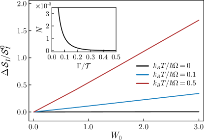
Figure 2: Partition noise and number of charges in a heat pulse. Electric noise is generated by heat pulses that are partitioned on the quantum point contact with $D=1/2$. We show the difference between the noise with and without the drive, $\Delta\mathcal{S}_{I}=\mathcal{S}_{I}^{\mathrm{on}}(0)-\mathcal{S}_{I}^{\mathrm{off}}(0)$, normalized by the noise of a single particle $\mathcal{S}^{0}_{I}=e^{2}fD(1-D)$, where $f$ is the driving frequency. The half-width of the Lorentzian pulses is $\Gamma=0.2\mathcal{T}$. At zero temperature, this ratio yields the number of electrons and holes in a pulse as shown in the inset for $W_{0}=0.2$.

Linear response.— We can also analyse the heat current in linear response to a cosine drive with $W_{0}\ll 1$. To first order in $W_{0}$, we then find $J(t)=\mathcal{G}(\Omega)W(t)$ with the frequency-dependent response to the driving field reading

$$\mathcal{G}(\omega)=\frac{(2\pi k_{B}T)^{2}+(\hbar\omega)^{2}}{12h}.$$ (6)

We can write the heat current as $J(t)=G_{Q}\Delta T(t)+(f\hbar\Omega/12)W(t)$, where $G_{Q}=\pi^{2}k_{B}^{2}T/3h$ is the thermal conductance quantum, and $\Delta T(t)=W(t)T$ is the temperature bias. At high temperatures, the heat current is mainly driven by the temperature bias. On the other hand, as the temperature is lowered, the second contribution becomes relevant, and at zero temperature, the heat pulses are generated directly by the driving field, since the thermal conductance quantum vanishes. The magnitude of the heat current is then given by the size of the modulation quanta, $\hbar\Omega$, times the frequency at which they are emitted, $f=1/\mathcal{T}$. Importantly, the second term in Eq. (6) ensures that the fluctuation-dissipation theorem for heat currents, whose validity has been debated [33, 34, 35], is fulfilled. Indeed, by evaluating the equilibrium noise of the heat current [56], we find $\mathcal{S}_{Q}(\omega)=\hbar\omega\mathrm{Re}[\mathcal{G}(\omega)]\coth{(\hbar\omega/2k_{B}T)}$ in accordance with the fluctuation-dissipation theorem [57]. It is instructive to compare Eq. (6) with the electric conductance of a ballistic conductor, which reads $e^{2}/h$ at all frequencies. Finally, we note that experiments with fast voltage pulses were conducted at temperatures below $T=50$ mK, corresponding to an energy of about $k_{B}T=0.4$ $\mu$eV, while the driving frequencies reached almost $\Omega=20$ GHz, corresponding to the energy $\hbar\Omega=80$ $\mu$eV [7, 8]. At such high frequencies and low temperatures, one would observe nonadiabatic effects according to Eq. (6).

Partition noise.— The absence of an electric current in a ballistic conductor demonstrates that the heat pulses are electrically neutral. To probe the number of electrons and holes in a heat pulse, we proceed as in recent experiments and evaluate the electric noise in the outputs of the quantum point contact with a finite transmission [7, 36]. While electrons and holes contribute with opposite signs to the electric current, they generate the same partition noise, when scattered on a quantum point contact. Specifically, at zero temperature, the low-frequency noise can be expressed as $\mathcal{S}_{I}(0)=N\mathcal{S}^{0}_{I}$ in terms of the number of charges in a heat pulse, $N=N_{e}+N_{h}$, where $\mathcal{S}^{0}_{I}=e^{2}fD(1-D)$ is the partition noise of a single particle. Thus, from the low-frequency noise in the outputs, we can extract the number of charges as $N=\mathcal{S}_{I}(0)/\mathcal{S}^{0}_{I}$. At finite temperatures, we define the excess noise as the difference between the noise with and without the drive, $\Delta\mathcal{S}_{I}=\mathcal{S}_{I}^{\mathrm{on}}(0)-\mathcal{S}_{I}^{\mathrm{off}}(0)$, as shown in Fig. 2 as a function of the driving amplitude, while the inset shows the number of electrons and holes in a pulse at zero temperature.

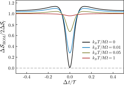
Figure 3: Hong-Ou-Mandel interferometry with heat pulses. Heat pulses arrive on each side of the quantum point contact with transmission $D=1/2$. We show the electric noise in the outputs as a function of a controllable time delay between the pulses. The parameters of the Lorentzian pulses are $W_{0}=0.1$ and $\Gamma=0.03\mathcal{T}$. At low temperatures, the noise is suppressed at zero time delay, showing that the heat pulses antibunch.

Hong–Ou–Mandel interferometry.— We now consider heat pulses that are emitted onto each side of the quantum point contact to realize a Hong-Ou-Mandel setup [37, 11, 7, 8, 58]. Specifically, we evaluate the electric noise in the outputs as a function of a phase difference between the two drives. Identical bosons that arrive simultaneously on each side of a beam splitter are expected to bunch and leave via the same output arm. Fermions, by contrast, tend to antibunch and exit via different output arms. While bunching leads to increased noise, antibunching reduces the noise. Figure 3 shows the excess noise for heat pulses that arrive on each side of the quantum point contact with a time delay between them. In this case, we normalize the noise with respect to the noise that is generated by pulses that arrive on only one side of the quantum point contact. When the pulses arrive simultaneously, we observe a clear suppression of the noise due to antibunching. The width of the suppression is given by the overlap of the pulses, and the suppression is gradually lifted as the temperature is increased. Small enhancements appear around the suppressed noise, which have also been predicted for Hong–Ou–Mandel experiments with electron-hole collisions [59, 60].

Mach–Zehnder interferometer.— The heat pulses are electrically neutral. However, we can generate an electric current using a Mach–Zehnder interferometer, which breaks the electron-hole symmetry and thereby enables a thermoelectric effect [38, 39]. We thus consider the interferometer in Fig. 4 with the scattering amplitude

$$S_{\mathrm{MZ}}(E)=r_{1}r_{2}e^{i(E\tau_{u}/\hbar+\phi_{u})}+t_{1}t_{2}e^{i(E\tau_{d}/\hbar+\phi_{d})}$$ (7)

for transmissions from the upper input to the upper output. Here, the reflection (transmission) amplitudes of the first and second quantum point contact are denoted by $r_{j}$ ($t_{j}$), $j=1,2$, the time that it takes to transverse the upper and lower paths is $\tau_{u}$ and $\tau_{d}$, while $\phi_{u}$ and $\phi_{d}$ are the phases that are picked up due to an applied magnetic field. For half-transmitting quantum point contacts, $r_{j},t_{j}=1/\sqrt{2}$, the transmission probability reads $T_{\mathrm{MZ}}(E)=|S_{\mathrm{MZ}}(E)|^{2}=[1+\cos(E\tau/\hbar+\Phi)]/2$, where $\tau=\tau_{u}-\tau_{d}$ is given by the path-length difference, and $\Phi=\phi_{u}-\phi_{d}$ is controlled by the enclosed magnetic flux. Importantly, the magnetic flux allows us to break the electron-hole symmetry, so that $T_{\mathrm{MZ}}(-E)\neq T_{\mathrm{MZ}}(E)$.

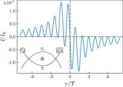
Figure 4: Mach–Zehnder interferometer and thermoelectric effect. Cosine pulses with amplitude $W_{0}$ are applied to the upper input of a Mach-Zenhder interferometer, and we show the average electric current in the upper output as a function of the path length difference to lowest order in the driving amplitude. The base temperature is zero. For non-zero fluxes and path-length differences, the electron-hole symmetry is broken, and a finite electric current is running in the upper output.

In Fig. 4, we show the average electric current in the upper output as a function of the path length difference. For a cosine drive, the electric current at zero temperature can be calculated to lowest order in the amplitude,

$$\bar{I}=I_{\Phi}\sin^{2}(\bar{\tau})\left[1-\bar{\tau}\cot(\bar{\tau})-\bar{\tau}^{2}/2\right]/(2\bar{\tau})^{3},$$ (8)

where we have defined $I_{\Phi}=W_{0}^{2}ef\sin(\Phi)$ and $\bar{\tau}=\pi\tau/\mathcal{T}$. From this expression, we see that an electric current indeed can be generated if a magnetic field is applied, so that $I_{\Phi}\neq 0$, and the current can be either positive or negative depending on the flux. The current also changes sign as $\bar{I}(-\tau)=-\bar{I}(\tau)$, and it vanishes for path length differences that match the period of the drive, $\tau=n\mathcal{T}$. In addition, there is no current for large path length differences. These results show how both the sign and the magnitude of the electric current can be controlled by the magnetic flux and the path length difference.

Conclusions.— We have presented a Floquet scattering theory of heat pulses in mesoscopic conductors. The pulses are generated in response to work that is performed on an electrode to change its temperature. We have found the response function for a ballistic conductor, which agrees with the fluctuation-dissipation theorem for heat currents. The pulses are uncharged, and the number of electrons and holes in a pulse can be determined from the partition noise after a quantum point contact. We have also found that the heat pulses antibunch when arriving simultaneously on each side of a quantum point contact. Finally, we have used a Mach-Zehnder interferometer to break the electron-hole symmetry and thereby enable a thermoelectric effect.

Our work paves the way for systematic investigations of dynamic heat transport in mesoscopic conductors, and it can be extended in many different directions. For example, it would be interesting to visualize the heat pulses using their Wigner representation. The influence of the pulse shape on the emitted pulses should also be explored. Since the heat pulses are electrically neutral, it is possible that they are less prone to interactions and decoherence effects, which is another question that deserves to be addressed. Finally, while we have mainly focused on the properties of the heat pulses themselves, it would be relevant to develop a microscopic description of how work is performed on an electrode to generate the pulses, for example by shining light on the electrode. These and other questions we leave for future work.

Acknowledgements.— We thank K. Brandner, P. Burset, K. Flensberg, C. Gorini, N. Lo Gullo, M. V. Moskalets, B. Roussel, and P. Samuelsson for useful discussions. We acknowledge support from Jane and Aatos Erkko Foundation and Research Council of Finland through Finnish Centre of Excellence in Quantum Technology (352925) and grant number 331737.

References

- Bocquillon et al. [2014] E. Bocquillon, V. Freulon, F. D. Parmentier, J.-M. Berroir, B. Plaçais, C. Wahl, J. Rech, T. Jonckheere, T. Martin, C. Grenier, D. Ferraro, P. Degiovanni, and G. Fève, Electron quantum optics in ballistic chiral conductors, Ann. Phys. 526, 1 (2014).
- Splettstoesser and Haug [2017] J. Splettstoesser and R. J. Haug, Single-electron control in solid state devices, Phys. Status Solidi B 254, 1770217 (2017).
- Bäuerle et al. [2018] C. Bäuerle, D. C. Glattli, T. Meunier, F. Portier, P. Roche, P. Roulleau, S. Takada, and X. Waintal, Coherent control of single electrons: a review of current progress, Rep. Prog. Phys. 81, 056503 (2018).
- Levitov et al. [1996] L. S. Levitov, H. Lee, and G. B. Lesovik, Electron counting statistics and coherent states of electric current, J. Math. Phys. 37, 4845 (1996).
- Ivanov et al. [1997] D. A. Ivanov, H. W. Lee, and L. S. Levitov, Coherent states of alternating current, Phys. Rev. B 56, 6839 (1997).
- Keeling et al. [2006] J. Keeling, I. Klich, and L. S. Levitov, Minimal Excitation States of Electrons in One-Dimensional Wires, Phys. Rev. Lett. 97, 116403 (2006).
- Dubois et al. [2013a] J. Dubois, T. Jullien, F. Portier, P. Roche, A. Cavanna, Y. Jin, W. Wegscheider, P. Roulleau, and D. C. Glattli, Minimal-excitation states for electron quantum optics using levitons, Nature 502, 659 (2013a).
- Jullien et al. [2014] T. Jullien, P. Roulleau, B. Roche, A. Cavanna, Y. Jin, and D. C. Glattli, Quantum tomography of an electron, Nature 514, 603 (2014).
- Ji et al. [2003] Y. Ji, Y. Chung, D. Sprinzak, M. Heiblum, D. Mahalu, and H. Shtrikman, An electronic Mach-Zehnder interferometer, Nature 422, 415 (2003).
- Ofek et al. [2010] N. Ofek, A. Bid, M. Heiblum, A. Stern, V. Umansky, and D. Mahalu, Role of interactions in an electronic Fabry–Perot interferometer operating in the quantum Hall effect regime, Proc. Natl. Acad. Sci. 107, 5276 (2010).
- Bocquillon et al. [2013] E. Bocquillon, V. Freulon, J.-M. Berroir, P. Degiovanni, B. Plaçais, A. Cavanna, Y. Jin, and G. Fève, Coherence and Indistinguishability of Single Electrons Emitted by Independent Sources, Science 339, 1054 (2013).
- Wang et al. [2023] J. Wang, H. Edlbauer, A. Richard, S. Ota, W. Park, J. Shim, A. Ludwig, A. D. Wieck, H.-S. Sim, M. Urdampilleta, T. Meunier, T. Kodera, N.-H. Kaneko, H. Sellier, X. Waintal, S. Takada, and C. Bäuerle, Coulomb-mediated antibunching of an electron pair surfing on sound, Nat. Nanotech. 18, 721 (2023).
- Fletcher et al. [2023] J. D. Fletcher, W. Park, S. Ryu, P. See, J. P. Griffiths, G. A. C. Jones, I. Farrer, D. A. Ritchie, H.-S. Sim, and M. Kataoka, Time-resolved Coulomb collision of single electrons, Nat. Nanotech. 18, 727 (2023).
- Ubbelohde et al. [2023] N. Ubbelohde, L. Freise, E. Pavlovska, P. G. Silvestrov, P. Recher, M. Kokainis, G. Barinovs, F. Hohls, T. Weimann, K. Pierz, and V. Kashcheyevs, Two electrons interacting at a mesoscopic beam splitter, Nat. Nanotech. 18, 733 (2023).
- Portugal et al. [2021] P. Portugal, C. Flindt, and N. Lo Gullo, Heat transport in a two-level system driven by a time-dependent temperature, Phys. Rev. B 104, 205420 (2021).
- Portugal et al. [2022] P. Portugal, F. Brange, and C. Flindt, Effective temperature pulses in open quantum systems, Phys. Rev. Res. 4, 043112 (2022).
- Chen et al. [2023] R. Chen, T. Gibson, and G. T. Craven, Energy transport between heat baths with oscillating temperatures, Phys. Rev. E 108, 024148 (2023).
- Dhar [2008] A. Dhar, Heat transport in low-dimensional systems, Adv. Phys. 57, 457 (2008).
- Battista et al. [2013] F. Battista, M. Moskalets, M. Albert, and P. Samuelsson, Quantum Heat Fluctuations of Single-Particle Sources, Phys. Rev. Lett. 110, 126602 (2013).
- Ludovico et al. [2014] M. F. Ludovico, J. S. Lim, M. Moskalets, L. Arrachea, and D. Sánchez, Dynamical energy transfer in ac-driven quantum systems, Phys. Rev. B 89, 161306 (2014).
- Pekola [2015] J. P. Pekola, Towards quantum thermodynamics in electronic circuits, Nat. Phys. 11, 118 (2015).
- Dashti et al. [2018] N. Dashti, M. Misiorny, P. Samuelsson, and J. Splettstoesser, Probing charge- and heat-current noise by frequency-dependent fluctuations in temperature and potential, Phys. Rev. Appl. 10, 024007 (2018).
- Pekola and Karimi [2021] J. P. Pekola and B. Karimi, Colloquium: Quantum heat transport in condensed matter systems, Rev. Mod. Phys. 93, 041001 (2021).
- Ferraro et al. [2014] D. Ferraro, B. Roussel, C. Cabart, E. Thibierge, G. Fève, C. Grenier, and P. Degiovanni, Real-Time Decoherence of Landau and Levitov Quasiparticles in Quantum Hall Edge Channels, Phys. Rev. Lett. 113, 166403 (2014).
- Samuelsson et al. [2017] P. Samuelsson, S. Kheradsoud, and B. Sothmann, Optimal Quantum Interference Thermoelectric Heat Engine with Edge States, Phys. Rev. Lett. 118, 256801 (2017).
- Li et al. [2023] M. Li, H. Wu, E. M. Avery, Z. Qin, D. P. Goronzy, H. D. Nguyen, T. Liu, P. S. Weiss, and Y. Hu, Electrically gated molecular thermal switch, Science 382, 585 (2023).
- Molenkamp et al. [1992] L. W. Molenkamp, T. Gravier, H. van Houten, O. J. A. Buijk, M. A. A. Mabesoone, and C. T. Foxon, Peltier coefficient and thermal conductance of a quantum point contact, Phys. Rev. Lett. 68, 3765 (1992).
- Chiatti et al. [2006] O. Chiatti, J. T. Nicholls, Y. Y. Proskuryakov, N. Lumpkin, I. Farrer, and D. A. Ritchie, Quantum Thermal Conductance of Electrons in a One-Dimensional Wire, Phys. Rev. Lett. 97, 056601 (2006).
- Jezouin et al. [2013] S. Jezouin, F. D. Parmentier, A. Anthore, U. Gennser, A. Cavanna, Y. Jin, and F. Pierre, Quantum Limit of Heat Flow Across a Single Electronic Channel, Science 342, 601 (2013).
- Banerjee et al. [2018] M. Banerjee, M. Heiblum, V. Umansky, D. E. Feldman, Y. Oreg, and A. Stern, Observation of half-integer thermal Hall conductance, Nature 559, 205 (2018).
- Melcer et al. [2023] R. A. Melcer, S. Konyzheva, M. Heiblum, and V. Umansky, Direct determination of the topological thermal conductance via local power measurement, Nat. Phys. 19, 327 (2023).
- Pendry [1983] J. B. Pendry, Quantum limits to the flow of information and entropy, J. Phys. A: Math. Gen. 16, 2161 (1983).
- Averin and Pekola [2010] D. V. Averin and J. P. Pekola, Violation of the Fluctuation-Dissipation Theorem in Time-Dependent Mesoscopic Heat Transport, Phys. Rev. Lett. 104, 220601 (2010).
- Zhan et al. [2011] F. Zhan, S. Denisov, and P. Hänggi, Electronic heat transport across a molecular wire: Power spectrum of heat fluctuations, Phys. Rev. B 84, 195117 (2011).
- Moskalets [2014a] M. Moskalets, Floquet Scattering Matrix Theory of Heat Fluctuations in Dynamical Quantum Conductors, Phys. Rev. Lett. 112, 206801 (2014a).
- Dubois et al. [2013b] J. Dubois, T. Jullien, C. Grenier, P. Degiovanni, P. Roulleau, and D. C. Glattli, Integer and fractional charge Lorentzian voltage pulses analyzed in the framework of photon-assisted shot noise, Phys. Rev. B 88, 085301 (2013b).
- Hong et al. [1987] C. K. Hong, Z. Y. Ou, and L. Mandel, Measurement of subpicosecond time intervals between two photons by interference, Phys. Rev. Lett. 59, 2044 (1987).
- Moskalets [2014b] M. Moskalets, Fermi-sea correlations and a single-electron time-bin qubit, Phys. Rev. B 90, 155453 (2014b).
- Gaury and Waintal [2014] B. Gaury and X. Waintal, Dynamical control of interference using voltage pulses in the quantum regime, Nat. Commun. 5, 3844 (2014).
- Moskalets [2011] M. V. Moskalets, Scattering Matrix Approach to Non-Stationary Quantum Transport (Imperial College Press, 2011).
- Brandner [2020] K. Brandner, Coherent Transport in Periodically Driven Mesoscopic Conductors: From Scattering Amplitudes to Quantum Thermodynamics, Z. Naturforsch. A 75, 483 (2020).
- [42] The Hamiltonian may be realized in different ways depending on the experimental setup. For example, close to the Fermi level, the Hamiltonian can be linearized as , and one might realize the full Hamiltonian as using appropriate ligth fields that couple to the momentum of the electrons [61, 62].
- Luttinger [1964] J. M. Luttinger, Theory of thermal transport coefficients, Phys. Rev. 135, A1505 (1964).
- Eich et al. [2014] F. G. Eich, A. Principi, M. Di Ventra, and G. Vignale, Luttinger-field approach to thermoelectric transport in nanoscale conductors, Phys. Rev. B 90, 115116 (2014).
- Tatara [2015] G. Tatara, Thermal Vector Potential Theory of Transport Induced by a Temperature Gradient, Phys. Rev. Lett. 114, 196601 (2015).
- Bhandari et al. [2020] B. Bhandari, P. T. Alonso, F. Taddei, F. von Oppen, R. Fazio, and L. Arrachea, Geometric properties of adiabatic quantum thermal machines, Phys. Rev. B 102, 155407 (2020).
- Arrachea [2023] L. Arrachea, Energy dynamics, heat production and heat–work conversion with qubits: toward the development of quantum machines, Rep. Prog. Phys. 86, 036501 (2023).
- López et al. [2023] R. López, P. Simon, and M. Lee, Heat and charge transport in interacting nanoconductors driven by time-modulated temperatures (2023), arXiv:2308.03426 .
- [49] The Supplemental Material contains technical details of our calculations.
- [50] A time-dependent voltage can be described by the Floquet scattering matrix [40] .
- Arrachea and Moskalets [2006] L. Arrachea and M. Moskalets, Relation between scattering-matrix and Keldysh formalisms for quantum transport driven by time-periodic fields, Phys. Rev. B 74, 245322 (2006).
- Hasegawa and Kato [2018] M. Hasegawa and T. Kato, Effect of interaction on reservoir-parameter-driven adiabatic charge pumping via a single-level quantum dot system, Journal of the Physical Society of Japan 87, 044709 (2018).
- Moskalets and Büttiker [2004] M. Moskalets and M. Büttiker, Floquet scattering theory for current and heat noise in large amplitude adiabatic pumps, Phys. Rev. B 70, 245305 (2004).
- Moskalets and Haack [2016] M. Moskalets and G. Haack, Heat and charge transport measurements to access single-electron quantum characteristics, Phys. Status Solidi 254, 1600616 (2016).
- Moskalets and Büttiker [2002] M. Moskalets and M. Büttiker, Floquet scattering theory of quantum pumps, Phys. Rev. B 66, 205320 (2002).
- Sergi [2011] D. Sergi, Energy transport and fluctuations in small conductors, Phys. Rev. B 83, 033401 (2011).
- Kubo [1957] R. Kubo, Statistical-Mechanical Theory of Irreversible Processes. I. General Theory and Simple Applications to Magnetic and Conduction Problems, J. Phys. Soc. Jpn. 12, 570 (1957).
- Ferraro et al. [2018] D. Ferraro, F. Ronetti, L. Vannucci, M. Acciai, J. Rech, T. Jockheere, T. Martin, and M. Sassetti, Hong-Ou-Mandel characterization of multiply charged Levitons, Eur. Phys. J. Spec. Top. 227, 1345 (2018).
- Jonckheere et al. [2012] T. Jonckheere, J. Rech, C. Wahl, and T. Martin, Electron and hole Hong-Ou-Mandel interferometry, Phys. Rev. B 86, 125425 (2012).
- Rech et al. [2016] J. Rech, C. Wahl, T. Jonckheere, and T. Martin, Electron interferometry in integer quantum Hall edge channels, J. Stat. Mech. 2016, 054008 (2016).
- Grifoni and Hänggi [1998] M. Grifoni and P. Hänggi, Driven quantum tunneling, Phys. Rep. 304, 229 (1998).
- Platero and Aguado [2004] G. Platero and R. Aguado, Photon-assisted transport in semiconductor nanostructures, Phys. Rep. 395, 1 (2004).