Morpho-kinematical modelling in the molecular zoo beyond CO: the case of M 1-92

Abstract

Ongoing improvements of sub-mm- and mm-range interferometers and single-dish radiotelescopes are progressively allowing the detailed study of planetary nebulae (PNe) in molecular species other than ¹²CO and ¹³CO. We are implementing a new set of tables for extending the capabilities of the morpho-kinematical modelling tool SHAPE+shapemol, so radiative transfer in molecular species beyond ¹²CO and ¹³CO, namely C¹⁷O, C¹⁸O, HCN, HNC, CS, SiO, HCO⁺, and N₂H⁺, are enabled under the Large Velocity Gradient approximation with the ease of use of SHAPE. We present preliminary results on the simultaneous analysis of a plethora of IRAM-30m and HERSCHEL/HIFI spectra, and NOEMA maps of different species in the pre-PN nebula M 1-92, which show interesting features such as a previously undetected pair of polar, turbulent, high-temperature blobs, or a ¹⁷O/¹⁸O isotopic ratio of 1.7, which indicates the AGB should have turned C-rich, as opposed to the apparent nature of its O-rich nebula.

1 Introduction

Over the last few decades, morpho-kinematical modelling of planetary nebulae (PNe) has provided a wealth of information useful for gaining insight into PN formation (e.g., Solf & Ulrich,, 1985; Santander-García et al.,, 2004; Akashi & Soker,, 2013, 2018). Parameters derived from these models include the current 3D geometry and 3D velocity field of the ejecta, as well as its spatial orientation and kinematical (distance-dependent) age. These allow for instance to establish the evolutionary sequence of formation in the case of a ejecta composed of multiple structures, or investigating whether the equator of the PNe is aligned with the orbital plane of a close-binary central star (as models predict, see e.g. Jones,, 2020), provided the latter is known.

Despite its proved usefulness, this kind of modelling has its limitations: it only provides a snapshot of the current state of the nebula, and it lacks information on other physical parameters necessary for hydrodynamic or magnetohydrodynamic modelling, such densities, temperatures and pressures at each location throughout the PN.

This shortcoming can be overcome, in the case of the molecular regime, by the inclusion of radiative transfer calculations of molecular species in these models. In this regard, the inclusion of shapemol (Santander-García et al.,, 2015) in the user-friendly, successful morphokinematical modelling code SHAPE (Steffen et al.,, 2011) enabled accurate non-LTE calculations of excitation and radiative transfer in ¹²CO and ¹³CO rotational lines under the Large Velocity Gradient (LVG) approximation (e.g. Castor,, 1970), producing both synthetic single-dish profiles and spectral maps to match observations. Simultaneous fitting of lines of low- and high-excitation in this manner allows to derive the excitation conditions of the gas, namely its density and temperature, as well as the abundance of each species relative to that of molecular hydrogen. These in turn lead to estimates of the mass of the molecule-rich region of the PNe, provides some insight about the conditions for molecular chemistry, and further informs models of formation of PNe.

We introduce the addition of several new molecular species in shapemol, as well as a code to better allow for direct matching of interferometric observations. We use these tools to show preliminary results on the simultaneous analysis of a plethora of IRAM-30m and HERSCHEL/HIFI spectra, and NOEMA interferometric maps of different species in the pre-PN M 1-92.

The work presented here will be further discussed in much deeper detail by Masa et al. (in preparation).

2 Expanding shapemol

The emission $j_{\nu}$ and absorption $k_{\nu}$ coefficients calculated by shapemol for each molecular species and individual transition rely on pre-generated tables according to the density $n$ of each model grid cell, its temperature $T$, and the product $X\times\frac{r}{V}$, where $X$ is the abundance of the species with respect to H₂, and $r$ and $V$ are the distance to the central star and the expansion velocity, respectively. Tables provided for the previous version of shapemol (Santander-García et al.,, 2015) spanned a range of physical parameters expected to be found in the circumstellar environment of evolved low- and intermediate-mass stars, allowing to model ejecta with $n$ in the range 10² – 10⁷ cm^-3, $T$ from 10 to 1000 K, and $X\times\frac{r}{V}$ in the range $2.5\times 10^{10}$ – $1.3\times 10^{13}$ cm km^-1 s, and $8.3\times 10^{8}$ – $4.2\times 10^{11}$ cm km^-1 s for ¹²CO and ¹³CO respectively. These coverage was more focused on modelling of PNe, and were therefore insufficient for some projects. Modelling Asymptotic Giant Branch (AGB) stars, for instance, represented quite a struggle. Consequently, the new version of shapemol considerably expands the table coverage for ¹²CO and ¹³CO by several orders of magnitude in $n$, and a broader range in $X\times\frac{r}{V}$.

In addition, we have expanded the capabilities of shapemol by including a whole new set of molecular species, namely C¹⁷O, C¹⁸O, HCN, HNC, CS, SiO, HCO⁺, and N₂H⁺. The preliminary parameter coverage in these molecules, as well as the new coverage for ¹²CO and ¹³CO, can be found in Table 1. Note that the parameter coverage is susceptible to expand in the final version presented in Masa et al. (in preparation). An illustrative example of the emission coefficient $j_{\nu}$ of HCN and HNC for a broad range of physical conditions is shown in Figure 1.

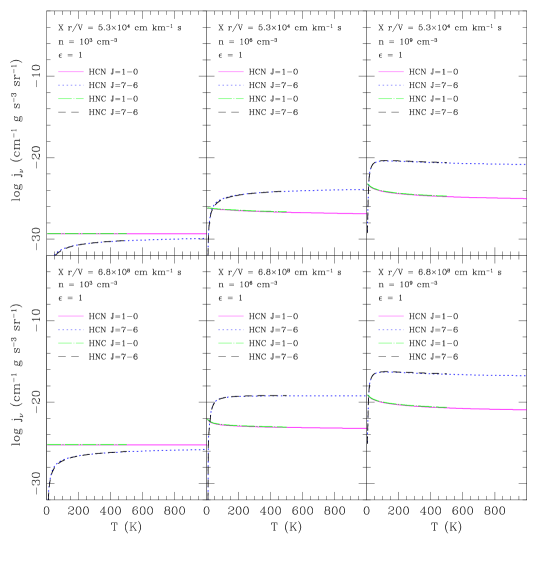
Figure 1: Example of the emission coefficient $j_{\nu}$ of HCN and HNC under a range of conditions of abundance, density and temperature (and a unique value of the logarithmic velocity gradient, $\epsilon=dV/dr~{}r/V$, corresponding to ballistic expansion.

The computed $j_{\nu}$ and $k_{\nu}$ were tested in two different manners. We first compared a simple, spherical model computed with SHAPE+shapemol with theoretical calculations of the optical depth $\tau$ under LVG conditions, finding typical errors of a few ‰ in the optically thin case, increasing to a few % as the nebula becomes optically thick. We also performed a battery of emission and absorption coefficients checks against the results provided by RADEX (Van Der Tak et al.,, 2007). Although RADEX is not a LVG code, the small offsets we found (with typical values of $\sim$5%) ensure our calculations are accurate enough.

Table 1: Molecules included and parameter coverage of the version of shapemol presented in this work.

Species	$n$ (cm-3)	$T$ (K)	$X\times\frac{r}{V}$ (cm km-1 s)
12CO	102 – 1012	5 – 1000	$1.2\times 10^{9}$ – $6.1\times 10^{13}$
13CO	102 – 1012	5 – 1000	$3.8\times 10^{7}$ – $2.0\times 10^{12}$
C17O	102 – 1012	5 – 1000	$2.3\times 10^{7}$ – $1.2\times 10^{12}$
C18O	102 – 1012	5 – 1000	$1.2\times 10^{7}$ – $6.1\times 10^{11}$
HCN	102 – 1012	5 – 1000	$5.0\times 10^{3}$ – $5.0\times 10^{10}$
HNC	102 – 1012	5 – 1000	$1.7\times 10^{3}$ – $1.7\times 10^{10}$
CS	102 – 1012	5 – 1000	$2.0\times 10^{4}$ – $1.1\times 10^{9}$
SiO	102 – 1012	5 – 1000	$5.0\times 10^{3}$ – $2.7\times 10^{8}$
HCO+	2.7$\times$102 – 1012⋆	5 – 1000	$5.0\times 10^{5}$ – $2.7\times 10^{10}$
N2H+	2.7$\times$102 – 1012⋆	5 – 1000	$5.0\times 10^{2}$ – $5.0\times 10^{9}$

Note: The lower limit of the coverage marked by $\star$ is planned to expand in the final version provided in Masa et al. (in preparation).

3 Proper comparison of synthetic models and interferometric observations

Interferometry involves emission filtering depending on the baselines and UV coverage. As a result, interferometric maps are not akin to Integral Field Spectroscopic data in the sense that they should not be compared with models in a direct fashion. Otherwise, flux lost in the observations (usually from extended, smooth structures) prevents a fair reconstruction by morpho-kinematical modelling.

Models simple enough (e.g. a flaring disk observed through an optical interferometer) can circumvent this limitation by direct comparison of model and observations in the UV plane. However, complex models with many parameters are a different story. In practice, comparisons are only possible in the image plane. Therefore, the model needs to undergo the same filtering and cleaning process suffered by the actual observations. This requires having accurate information of the interferometer configuration, baselines, etc., as well as of the source position in the sky at the moment(s) of observation. Essentially, we need the UV tables of the observation in order to apply the same filtering and cleaning process to the morpho-kinematical model. A proper comparison would also include the application of random noise similar to that of the observations to ensure an even better direct comparison.

We have devised a code for the radioastronomy GILDAS suite that allows to quickly apply this process to models exported from SHAPE, provided the UV table of the observation is available.

4 Preliminary model of M 1-92

In order to illustrate the new capabilities of SHAPE+shapemol as well as the aforementioned GILDAS code, we present a preliminary morpho-kinematical model of the pre-PN M 1-92. We use it to simultaneously fit NOEMA interferometric maps of the $J$=2$-$1 transition of ¹³CO, C¹⁷O, C¹⁸O, HCN, and HCO⁺, as well as a large number of single-dish observations from different species made with the IRAM 30 radiotelescope and HERSCHEL/HIFI, namely ¹²CO ($J$=1$-$0, $J$=2$-$1, $J$=5$-$4, $J$=7$-$6, $J$=9$-$8); ¹³CO, C¹⁷O and C¹⁸O ($J$=1$-$0, $J$=2$-$1); HNC and N₂H⁺ ($J$=1$-$0, $J$=3$-$2); HCN and HCO⁺ ($J$=1$-$0, $J$=2$-$1, $J$=3$-$2); CS ($J$=2$-$1, $J$=3$-$2); and SiO ($J$=2$-$1, $J$=3$-$2, $J$=4$-$3, $J$=5$-$4, $J$=6$-$5). We have kept the number of parameters down to a reasonable value in order to provide a comprehensive description of the geometry, motion, and physical conditions of the real ejecta.

A model sketch of this bipolar pre-PN is shown in Figure 2. A preliminary fit to different single-dish spectral profiles and interferometric maps can be seen in Figures 3, 4, and 5.

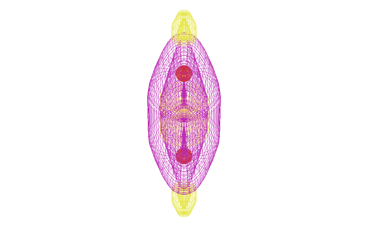
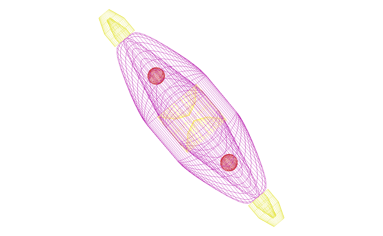
Figure 2: Sketch of the preliminary morpho-kinematical model of M 1-92 presented in this work.

The modelling so far suggests that the tapered shape of the nebula is topped by two polar tips carved out by a hot polar outflow. The inner and outer regions of these tips have very different physical conditions. The density of the model ranges from 1.8$\times$10⁵ cm^-3 in the equatorial inner region to a mere 10⁴ cm^-3 in the inner region of the polar tips, which also are the hotter ones of the model, at $\sim$450 K, as opposed to the much colder walls of the nebula at 17 K. The nebula expands homologously, except for a couple of small, dense and hot blobs half way along the main axis which dash through the nebula at a much higher velocity (55 km s^-1) than the surrounding regions. These blobs, as well as the polar tips, are significantly bright in HCO⁺and HCN, but difficult to tell apart in low-$J$ ¹²CO and ¹³CO transitions.

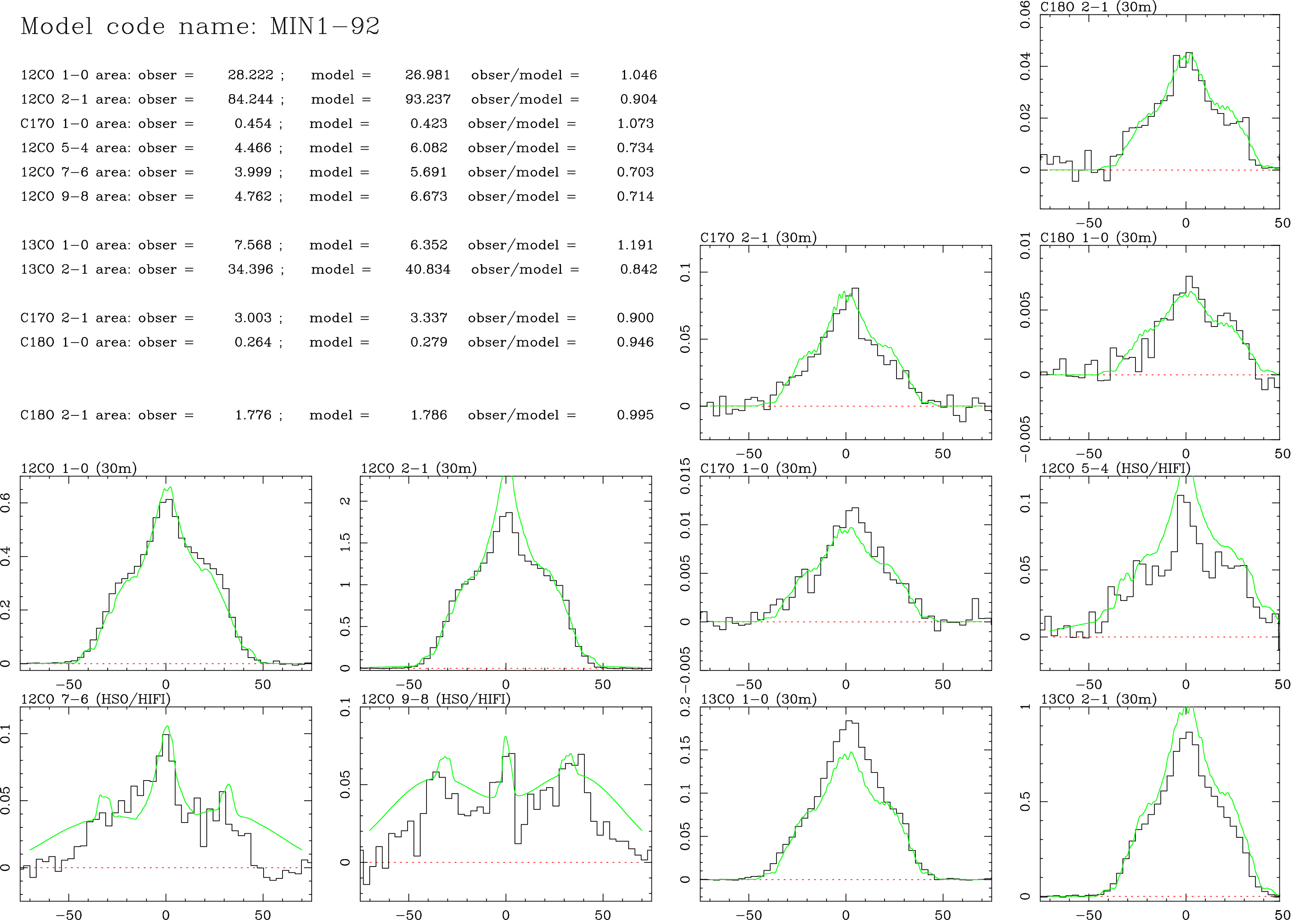
Figure 3: Preliminary model fit to different single-dish spectral profiles from ¹²CO, ¹³CO, C¹⁷O, and C¹⁸O in M 1-92. Numbers in the top left section refer to integrated intensities of both the observation and model in each line, as well as their ratio in order to better assess the fairness of the fit.

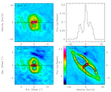
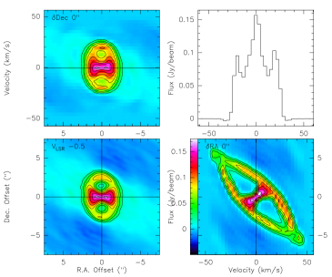
Figure 4: Left: A four-panel sample of the ¹³CO $J$=2$-$1 NOEMA interferometric observations of the pre-PN M 1-92. The central (systemic velocity) channel of the spectral map is shown in the bottom left panel. The top left and bottom right panels show position velocity maps along the horizontal and vertical directions, respectively. The top right panel shows the spectral profile at the central position. Right: Same for the preliminary model of M 1-92, after application of the GILDAS code to allow direct comparison with the observations.

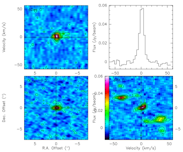
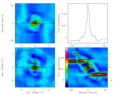
Figure 5: Left: A four-panel sample of the HCN $J$=2$-$1 NOEMA interferometric observations of the pre-PN M 1-92. The central (systemic velocity) channel of the spectral map is shown in the bottom left panel. The top left and bottom right panels show position velocity maps along the horizontal and vertical directions, respectively. The top right panel shows the spectral profile at the central position. Right: Same for the preliminary model of M 1-92, after application of the GILDAS code to allow direct comparison with the observations.

In summary, the data suggests an active chemistry is taking place in shocked, hot regions within M 1-92. Additionally, an ¹⁷O/¹⁸O isotopic ratio of 1.7 indicates the progenitor AGB should have turned carbon-rich during its evolution towards the tip of the AGB, whereas the resulting nebula is oxygen-rich. This discrepancy can be removed if the evolution of the AGB was suddenly interrupted by the event that gave rise to the current nebula in a sudden ejection, either by a close binary in common envelope or some other similar phenomenon.

A full description of the final version of this model will be given in Masa et al. (in preparation).

We acknowledge funding from the Spanish Ministry of Science and Innovation (MICINN) through project EVENTs/Nebulae-Web (grant PID2019-105203GB-C21).

References

- Akashi & Soker, (2013) Akashi, M., Soker, N., 2013, MNRAS, 436, 1961. doi: 10.1093/mnras/stt1704
- Akashi & Soker, (2018) Akashi, M., Soker, N., 2013, MNRAS, 481, 2754. doi:10.1093/mnras/sty2479
- Castor, (1970) Castor, J. I., 1970, MNRAS, 149, 111.
- Jones, (2020) Jones, D., 2020, Observational Constraints on the Common Envelope Phase, in Reviews in Frontiers of Modern Astrophysics: From Space Debris to Cosmology (eds. Kabath, Jones and Skarka; publisher Springer Nature), 123–153. doi:10.1007/978-3-030-38509-5_5
- Santander-García et al., (2004) Santander-García, M., Corradi, R. L. M., A. Mampaso, B. Balick, 2004, A&A, 426, 185. doi:10.1051/0004-6361:20041147
- Santander-García et al., (2015) Santander-García, M., Bujarrabal, V., Koning, N., Steffen, W., 2015, A&A, 573, 56. doi:10.1051/0004-6361/201322348
- Solf & Ulrich, (1985) Solf, J., Ulrich, H., 2022, A&A, 148, 274.
- Steffen et al., (2011) Steffen, W., Koning, N., Wenger, S., Morisset, C., Magnor, M., 2011, IEEE Transactions on Visualization and Computer Graphics, 17, 454. doi:10.1109/TVCG.2010.62
- Van Der Tak et al., (2007) Van Der Tak, F. F. S., Black, J. H., Schöier, F. L., Jansen, D. J., van Dishoeck, E. F., 2007, A&A, 468, 627. doi:10.1051/0004-6361:20066820