A Multivariate Unimodality Test Harnessing the Dip Statistic of Mahalanobis Distances Over Random Projections

Abstract

Unimodality, pivotal in statistical analysis, offers insights into dataset structures and drives sophisticated analytical procedures. While unimodality’s confirmation is straightforward for one-dimensional data using methods like Silverman’s approach and Hartigans’ dip statistic, its generalization to higher dimensions remains challenging. By extrapolating one-dimensional unimodality principles to multi-dimensional spaces through linear random projections and leveraging point-to-point distancing, our method, rooted in $\alpha$-unimodality assumptions, presents a novel multivariate unimodality test named mud-pod. Both theoretical and empirical studies confirm the efficacy of our method in unimodality assessment of multidimensional datasets as well as in estimating the number of clusters.

1 Introduction

Unimodality, a fundamental concept in statistical analysis, serves as a critical lens through which one can decipher the inherent structure and patterns within datasets. Understanding unimodality is paramount for multiple reasons. Firstly, it provides a rudimentary insight into the nature of the data, highlighting whether the data points converge towards a common central tendency or deviate significantly. Secondly, unimodality serves as a precursor to more complex analytical procedures, such as clustering algorithms, determining their necessity, and potentially influencing their outcomes (Kalogeratos & Likas, 2012; Daskalakis et al., 2013, 2014). In essence, the importance of unimodality transcends mere statistical significance, extending its value to practical, real-world applications.

In one-dimensional data, unimodality can be fundamentally understood as the task of discerning whether a given distribution exhibits a single prominent peak or mode. A notable advantage is that one-dimensional unimodality can be confirmed using robust statistical hypothesis tests, particularly for one-dimensional data. Methods such as Silverman’s approach, exploiting fixed-width kernel density estimates (Silverman, 1981), the widely recognized Hartigans’ dip statistic (Hartigan & Hartigan, 1985) and more recently the UU-test (Chasani & Likas, 2022) are prime examples.

Nevertheless, when transitioning to higher dimensions, the process of defining unimodality becomes less straightforward, even when considering only symmetric distributions. The intricacies of multi-dimensional spaces impose challenges that are not present in one-dimensional settings, leading to diverse interpretations and approaches to gauge unimodality. Even worse, these intricacies make the generalization of unimodality tests notably challenging. Numerous efforts have been made to capture the geometric essence of unimodality in $\mathbb{R}^{d}$ ($d>1$) and translate it into an analytical framework (Dai, 1989). In a seminal work by Olshen & Savage (1970), a definition of generalized unimodality characterized by a positive parameter $\alpha$ was proposed (called $\alpha$-unimodality), which is pertinent to distributions across $\mathbb{R}^{d}$ and offers a broader perspective that encompasses many aspects of 1-dimensional unimodality (Dharmadhikari & Joag-Dev, 1988, Chapter 3.2). Despite the various definitions, however, few methods are available for assessing unimodality in multidimensional data vectors.

In parallel, another line of research has delved into the use of random projections as a strategy for capturing the essence of multi-dimensional distributions. Random projections, known for its efficacy in dimensionality reduction, have shown significant potential for learning mixtures of Gaussians (Dasgupta, 1999). Additionally, the Diaconis-Freedman effect elucidates the behavior of random projections of probability distributions in the high-dimensional space (Diaconis & Freedman, 1984). Specifically, for a given probability distribution $P$ in a $d$-dimensional space, when we consider a dimension $q$ much smaller than $d$, the majority of the $q$-dimensional projections of $P$ resemble scaled mixtures of spherically symmetric Gaussian distributions (Dümbgen et al., 2013). Consequently, random projections appear to be a potent tool for the analysis of unimodality as they facilitate the transformation of the problem into a seemingly simpler space.

In this paper, we introduce an algorithm intertwining random projections with the notion of $\alpha$-unimodality to devise a robust technique for multivariate unimodality testing. Central to our investigation is the extrapolation of one-dimensional unimodality principles to multi-dimensional domains via random projections and point-to-point distancing. Our method relies on the notion of $\alpha$-unimodality. We demonstrate that linear random projections preserve the $\alpha$-unimodality property in Mahalanobis distances from a reference point. Leveraging these one-dimensional Mahalanobis distances, we apply the dip test for unimodality detection. Employing various random projections, akin to Monte Carlo simulations, we assess the $\alpha$-unimodality of the original data distribution. In summary, the contribution of our work is two-fold. Firstly, we propose the first mathematically founded multivariate unimodality test, dubbed mud-pod. Secondly, we present the mp-means incremental clustering method which is a wrapper around k-means exploiting mudpod for unimodality assessment. Both theoretical findings and empirical validations underpin our methods, showcasing efficacy in unimodality assessments and clustering scenarios.

2 Related Work

A multivariate unimodality test that aligns closely with our work is the dip-dist, introduced by Kalogeratos & Likas (2012). This criterion aims to ascertain the modality (unimodal vs. multimodal) of a dataset by applying the unidimensional dip test on each row of the pairwise distance matrix of the dataset. The rationale behind this approach is that by selecting an arbitrary data point and calculating its distances to all other points, we obtain a snapshot of the underlying cluster morphology. In presence of a single cluster, the distribution of distances is expected to be unimodal. To further the applicability of this criterion, it has been integrated into a clustering method named dip-means. This incremental algorithm employs cluster splitting based on the dip-dist to determine if a cluster should be divided. Consequently, dip-means can automatically estimate the cluster count. However, the dip-dist criterion is not without its limitations. A glaring drawback is its reliance on pairwise distances and its operation within the original data space, which can present challenges in certain scenarios. Moreover, the dip-dist method operates in an ad-hoc manner, lacking a rigorous mathematical foundation. In our work, we address these limitations by introducing random projections to assess unimodality on randomly projected distances. This approach permits Monte Carlo hypothesis testing by enabling sampling, previously not directly feasible in the original space. Additionally, we leverage the Mahalanobis distance and we empirically demonstrate its added benefits. Last but not least, we provide a mathematical formulation and prove the consistency of our test, thereby establishing the missing foundation for the dip-dist method.

The folding test, introduced in (Siffer et al., 2018), offers a versatile evaluation method suitable for both univariate and multivariate scenarios. This test revolves around the concept of folding, involving three key steps: (a) folding the distribution with respect to a designated pivot $s$, (b) calculating the variance of the folded distribution, and lastly, (c) comparing this folded variance to the original variance. The central idea behind the folding test is that when applied to multimodal distributions, the folded distribution typically exhibits a significantly reduced variance compared to its unimodal counterparts. A limitation of the folding test is its reliance on the empirical assumption that folding a multimodal distribution leads to a reduction in variance. Consequently, the concept of unimodality is not explicitly integrated into the folding test computation. It is important to note that there are cases where this assumption does not hold true, resulting in incorrect outcomes for the folding test (Chasani & Likas, 2022). Another research direction focuses on examining particular families of unimodal distributions. In the work of Dunn et al. (2021), a scalable test for log-concavity is elucidated building on maximum likelihood estimation (MLE), validated in finite samples across any dimension. A noteworthy empirical observation from their research is the pronounced efficacy achieved by adopting random projections. However, it is crucial to acknowledge that while log-concave functions capture a substantial subset of unimodal functions, they fall short of encompassing the entirety of the concept and may struggle to extend their applicability to more diverse and real-world scenarios.

3 Methods

3.1 Preliminaries

In the following we introduce some definitions and additional notation that we will use throughout the paper. We use capital letters to denote random variables or matrices and boldface type to represent vectors.

3.1.1 $\alpha$-Unimodal Distrubutions

Without loss of generality, we assume that the mode of the unimodal distribution is at $\mathbf{0}$. A random d-vector $\mathbf{X}\in\mathbb{R}^{d}$ is said to have an $\alpha$-unimodal distrubution about $\mathbf{0}$ if, for every bounded, nonnegative, Borel measurable function $g$ on $\mathbb{R}^{d}$ the quantity $t^{\alpha}\operatorname{\mathbb{E}}[g(t\mathbf{X})]$ is nondecreasing in $t\in(0,\infty)$. In what follows, we use the notation $\mathbf{X}\sim\mathcal{P_{\alpha}}$ to represent a d-vector following an $\alpha$-unimodal distribution. It follows from the defintion that if $\mathbf{X}\sim\mathcal{P_{\alpha}}$ and $\alpha<\beta$, then $\mathbf{X}\sim\mathcal{P_{\beta}}$. An important result that provides an equivalent characterization for the set of $\alpha$-unimodal distrubutions is the Decomposition theorem: $\mathbf{X}\sim\mathcal{P_{\alpha}}$ iff $\mathbf{X}$ is distributed as $U^{\frac{1}{\alpha}}\mathbf{Z}$ where $U$ is uniform on $(0,1)$ and $\mathbf{Z}$ is independent of U (Olshen & Savage, 1970).

This theorem closely mirrors the intuition of one-dimensional unimodality, since Khintchine (1938) demonstrated that a real random variable $X$ has a unimodal distribution iff $X\sim UZ$, where $U$ is uniform on $[0,1]$ and $U$ and $Z$ are independent. It follows that a scalar $X\sim\mathcal{P_{\alpha}}$ iff $X^{\alpha}$ is unimodal as per the standard definition in $\mathbb{R}$. Next, we present and prove three pivotal properties of $\alpha$-unimodal distributions, i.e., the translation, norm, and projection properties.

Lemma 1 (Translation Property).

Let $\mathbf{X}\sim\mathcal{P_{\alpha}}$ and $\mathbf{c}\in\mathbb{R}^{d}$, then $\mathbf{X}+\mathbf{c}\sim\mathcal{P_{\alpha}}$ .

• Let $t^{\alpha}\operatorname{\mathbb{E}}[g(t\mathbf{X}+t\mathbf{c})]=t^{\alpha}\operatorname{\mathbb{E}}[h(t\mathbf{X})]$, where $h(\mathbf{x})=g(\mathbf{x}+\mathbf{c})$. Note that $h$ is bounded, nonnegative, Borel measurable and that the first expression is nondecreasing iff the last expression is nondecreasing in $t$. $\blacksquare$

Lemma 2 (Norm Property).

Let $\mathbf{X}\sim\mathcal{P_{\alpha}}$, then $||\mathbf{X}||\sim\mathcal{P_{\alpha}}$.

• $||\mathbf{X}||=\sqrt{(U^{\frac{1}{\alpha}}\mathbf{Z})^{\top}(U^{\frac{1}{\alpha}}\mathbf{Z})}=U^{\frac{1}{\alpha}}||\mathbf{Z}||$ $\blacksquare$

Lemma 3 (Projection Property).

Let $\mathbf{X}\sim\mathcal{P_{\alpha}}$ and let $A$ be a real matrix from $\mathbb{R}^{d}$ to $\mathbb{R}^{q}$, then $A\mathbf{X}\sim\mathcal{P_{\alpha}}$.

• A direct use of the Decomposition Theorem. $\blacksquare$

Leveraging the foundational properties described above, we now present a salient result. This result not only fortifies our understanding of $\alpha$-unimodal distributions but will also play an instrumental role in the rest of the paper.

Lemma 4 (Mahalanobis).

Let $\mathbf{X}\sim\mathcal{P_{\alpha}}$ with a well-defined covariance matrix $\Sigma$ and $\mathbf{o}\in\mathbb{R}^{d}$, then the distribution of the Mahalanobis distances with respect to $\mathbf{o}$, given by $\sqrt{(\mathbf{X}-\mathbf{o})^{\top}{\Sigma}^{-1}(\mathbf{X}-\mathbf{o})}$ is $\alpha$-unimodal.

• Given a positive semidefinite covariance matrix $\Sigma$, and utilizing the matrix square root decomposition, the Mahalanobis distance can be expressed as:

  $$\sqrt{(\mathbf{x}-\mathbf{o})^{\top}\Sigma^{-1}(\mathbf{x}-\mathbf{o})} =||{\Sigma}^{-\frac{1}{2}}(\mathbf{x}-\mathbf{o})||$$

  The proof arises from translation and projection lemmas. $\blacksquare$

The Mahalanobis distance possesses distinct properties: it is unitless, scale-invariant, and comprehensively considers the covariance structure across all dimensions. Traditionally, it has been employed in multivariate hypothesis testing. Notably, the Hotelling’s $T^{2}$ statistic (Hotelling, 1931), which generalizes the Student’s t-statistic, exemplifies its usage. In our study, the Mahalanobis distance is pivotal to our multivariate unimodality test.

3.1.2 Dip Test

The dip test serves as a tool for discerning multimodality within a unidimensional dataset. It gauges this by examining the maximum deviation between the empirical distribution function and the closest unimodal distribution function. The dip statistic for a distribution function $F$ is defined as: $\text{dip}(F)=\min_{G\in U}\rho(F,G)$, where $\rho(F,G)=\max_{t}|F(t)-G(t)|$ and $U$ represents the set of all possible unimodal distributions.

The dip test’s significance is highlighted by its ability to unveil the least among the most substantial deviations between the empirical cumulative distribution function (e.c.d.f.) $F$ of the univariate dataset and the c.d.f.s of the class of unimodal distributions. A salient attribute of the dip statistic is its convergence as the sample size burgeons, such that $\lim_{{n\to\infty}}\text{dip}(F_{n})=\text{dip}(F)$ (Hartigan & Hartigan, 1985). Moreover, the class of uniform distributions $U$ is acclaimed to be the most fitting for the null hypothesis, owing to its stochastically larger dip values compared to other unimodal distributions. The p-value for unimodality, derived via bootstrap samples, functions as a determinant for the dataset’s modality. A dataset with a p-value greater than $a$ indicates unimodality; otherwise, multimodality is suggested.

3.1.3 Random Projections

The Diaconis-Freedman effect is a valuable tool for unimodality analysis, simplifying the problem by likely transforming it into a Gaussian mixture model. When considering a probability distribution $P$ in a $d$-dimensional space with a lower-dimensional focus $q\ll d$, most $q$-dimensional projections of $P$ resemble scale mixtures of spherically symmetric Gaussian distributions. Additionally, linear random projections can approximate inter-point distances when projecting high-dimensional points into lower-dimensional spaces. This phenomenon is encapsulated in the celebrated Johnson & Lindenstraus lemma presented below (Johnson & Lindenstraus, 1984; Fernandez-Granda, 2016):

JL Lemma: Let $S:=\{x_{i}\}_{i=1}^{k}$ be a subset of $\mathbb{R}^{d}$. There exists a scaled random Gaussian matrix $\Pi\in\mathbb{R}^{d\times q}$ with $\Pi_{ij}\sim\mathcal{N}(0,1)$, where $m\geq\frac{8\log(k)}{\epsilon^{2}}$, ensuring for any $x_{i},x_{j}\in S$ with probability at least $\mathit{1/k}$:

$$(1-\epsilon)\|x_{i}-x_{j}\|^{2}\leq\|\Pi x_{i}-\Pi x_{j}\|^{2}\leq(1+\epsilon)\|x_{i}-x_{j}\|^{2}$$

We define $\mathcal{R}_{\mathbf{\Pi}}$ to be the set of all random projections satisfying the conditions of the Johnson–Lindenstrauss lemma. By employing a square root decomposition, we can demonstrate the applicability of the Johnson-Lindenstrauss lemma to the Mahalanobis distance (Bhattacharya et al., 2009), while mitigating the singularity issue inherent in inverting the covariance matrix in high dimensions (Lopes et al., 2011; Radhendushka Srivastava & Ruppert, 2016).

3.2 Connecting the Dots

Given a dataset of multidimensional data vectors, assessing its unimodality becomes intricate. Random projections offer a solution by maintaining key pairwise distances and performing unimodality assessment in a more Gaussian-like space. By picking an arbitrary observer data point and deriving its distances to all other points, we garner a snapshot of the underlying cluster morphology. In presence of a single cluster, the distribution of distances is proven to be unimodal. Notably, the narrative this observer presents is contingent upon its location. We integrate this idea of random projection and the observer’s perspective into what we term a view. Our proposed algorithm focuses on analyzing these views, pinpointing those views that contradict unimodal narratives, and thus highlight multifaceted cluster formations. In the rest of the section, we will rigorously define the aforementioned concept.

Given a set $\mathcal{S}_{\mathbf{X}}$ of points from $\mathbf{X}\sim\mathcal{P_{\alpha}}$, let $\mathbf{o}\in\mathcal{S}_{\mathbf{X}}$ be a random point, dubbed observer. We define the set of Mahalanobis distances with regard to this observer as follows:

$$\mathcal{D}_{\mathbf{S}}^{o}=\left\{||{\mathbf{\Sigma}}^{-\frac{1}{2}}(\mathbf{x}-\mathbf{o})||\text{ }|\text{ }\mathbf{x}\in\mathcal{S}_{\mathbf{X}}\setminus\{\mathbf{o}\}\right\}.$$

Let $\Pi\in\mathcal{R}_{\mathbf{\Pi}}$, we define $\Pi\circ\mathcal{D}_{\mathbf{S}}^{o}$ to be the set of the Mahalanobis distances of the randomly projected points with respect to an observer $\mathbf{o}$. Specifically, we have:

$$\Pi\circ\mathcal{D}_{\mathbf{S}}^{o}=\left\{||{\mathbf{\Sigma}}^{-\frac{1}{2}}_{\Pi}\Pi(\mathbf{x}-\mathbf{o})||\text{ }|\text{ }\mathbf{x}\in\mathcal{S}_{\mathbf{X}}\setminus\{\mathbf{o}\}\wedge\Pi\in\mathcal{R}_{\mathbf{\Pi}}\right\},$$

where $\mathbf{\Sigma_{\Pi}}=\Pi\mathbf{\Sigma}\Pi^{T}$. It is important to note that given $\mathbf{X}\sim\mathcal{P_{\alpha}}$, both $\mathcal{D}_{\mathbf{S}}^{o}$ and $\Pi\circ\mathcal{D}_{\mathbf{S}}^{o}$ are $\alpha$-unimodal for any linear random projection $\Pi\in\mathcal{R}_{\mathbf{\Pi}}$, as established earlier. This yields the subsequent observation.

Proposition 1 (Randomisation Hypothesis).

Given the hypothesis that $\mathbf{X}\sim\mathcal{P_{\alpha}}$, $\mathcal{D}_{\mathbf{S}}^{o}$ is invariant under transformations in $\mathcal{R}_{\mathbf{\Pi}}$, ensuring that both $\mathcal{D}_{\mathbf{S}}^{o}$ and $\Pi\circ\mathcal{D}_{\mathbf{S}}^{o}$ exhibit an $\alpha$-unimodal distribution for any $\Pi\in\mathcal{R}_{\mathbf{\Pi}}$.

The Randomisation Hypothesis (RH) is central to our analysis. RH facilitates the execution of a series of one-dimensional unimodality tests, subsequently allowing the evaluation of the $\alpha$-unimodality of the distribution that produces our data $X$. Under the RH, every randomly projected distances should exhibit unimodality. Any deviation from this expected behavior can signal a departure from unimodality in the original data distribution. Random projections confer several distinct merits. Firstly, they preserve the pairwise distances, as endorsed by the JL lemma. Secondly, given our observations, random projections serve as an invaluable tool for unimodality investigation. They transmute the challenge into a space resembling a mixture of Gaussians. Furthermore, they ameliorate the singularity problem associated with the inversion of the covariance matrix used by the Mahalanobis distance. Lastly, they pave the way for harnessing Monte Carlo simulation for hypothesis testing (Lehmann & Romano, 2005), i.e., they establish the bedrock for sampling from a distribution, specifically $\mathcal{R}_{\mathbf{\Pi}}$, that is ostensibly simpler than the original data distribution of $\mathbf{X}$.

3.3 Multivariate Unimodality Testing

Building on the aforementioned foundation, we now introduce our multivariate $\alpha$-unimodality test called mud-pod. For a given $\alpha$ and a set of points $\mathcal{S}_{\mathbf{X}}$ from $\mathbf{X}\sim\mathcal{P_{\alpha}}$, we define our hypotheses:

$$H_{0} :\mathbf{X}\sim\mathcal{P_{\alpha}}\quad\text{vs}\quad H_{1}:\mathbf{X}\not\sim\mathcal{P_{\alpha}}$$

We define the pairing of a random projection $\Pi$ with an observer $\mathbf{o}$ as a random view. Given a set of $N$ random vectors $\mathcal{S}$ and a random view, we can obtain the corresponding set of Mahalanobis distances $\Pi\circ\mathcal{D}_{\mathbf{S}}^{o}$. Under the null hypothesis, recall that $\Pi\circ\mathcal{D}_{\mathbf{S}}^{o}=\{d_{i}\}_{i=1}^{N-1}$ is $\alpha$-unimodal, and the set $\{d_{i}^{\alpha}\}_{i=1}^{N-1}$ is unimodal, allowing the employment of the dip test. Let $T(\Pi\circ\mathcal{D}_{\mathbf{S}}^{o})$ denote the dip test p-value. If $a\in[0,1]$ is the significance level, the null hypothesis is rejected iff $T(\Pi\circ\mathcal{D}_{\mathbf{S}}^{o})\leq a$.

Utilizing the idea of random views, which, as previously discussed, preserve $\alpha$-unimodality, we can employ them as a foundation for Monte Carlo simulations. The rationale is that as more views reject the null hypothesis, our confidence about data multimodality increases. Let $\{\Pi_{i}\}_{i=1}^{M}\subset\mathcal{R}_{\mathbf{\Pi}}$ be a set of $M$ random projections. Leveraging Monte Carlo hypothesis testing theory (Lehmann & Romano, 2005, Chapter 11.2.2) and building on the fact that the dip statistic has a well defined c.d.f. (Hartigan & Hartigan, 1985), we explore the conditional c.d.f. of the dip test: $J_{N}(t)=P\left(T(\Pi\circ\mathcal{D}_{\mathbf{S}}^{o})\leq t\mid\mathcal{D}_{\mathbf{S}}^{o})\right)$. The aforementioned probability is measured over the joint distribution of random projections $\mathcal{R}_{\mathbf{\Pi}}$ and the distribution of observers $\mathcal{O}$. Let $I\{.\}$ denote the indicator function, we define $\hat{J}_{n,M}(t)$ as the approximation of the true c.d.f $J_{N}(t)$ computed on the series of the random views:

$$\hat{J}_{N,M}(t)=M^{-1}\sum_{i=1}^{M}I\left\{T(\Pi\circ\mathcal{D}_{\mathbf{S}}^{o})\leq t\right\}$$

By a direct application of the Glivenko-Cantelli theorem, we have that $\hat{J}_{N,M}(t)$ converges w.p. 1 to $J_{N}(t)$ (Sharipov, 2011). Interestingly, the Dvoretsky, Kiefer, Wolfowitz inequality provides bounds on the closeness between $\hat{J}_{N,M}(t)$ and $J_{N}(t)$ for a given $M$. Specifically, we have:

$$P\left(\sup_{t\in\mathbb{R}}|\hat{J}_{N,M}(t)-J_{N}(t)|>\tau\right)\leq Ce^{-2M\tau^{2}}$$

Hitherto, we have not delineated the methodology for selecting observers from the set of points obtained from a random projection. Several sampling strategies can exist, with the most intuitive being uniform random sampling. However, empirical results suggest that uniformly selecting observers based on a specific percentile of the distance distribution from the samples’ mean yields superior performance. The underlying rationale is that points situated farther away from the means possess a better capability to discern the topographical elevations formed by distinct clusters (Kalogeratos & Likas, 2012). Ultimately, the projection dimension is the minimal integer that satisfies the JL lemma for a specified $\epsilon$. For a given distribution family $\mathcal{P_{\alpha}}$, the complete mud-pod test is detailed in Algorithm 1.

Algorithm 1 mud-pod ($\alpha$, $X$, $a$, $M$, $p$, $\epsilon$)

Input: $\alpha$ (the positive unimodality index), $X$ (a set of real vectors), $a$ (a significance threshold), $M$ (number of simulations), $p$ (p-th percentile), $\epsilon$ (distance distortion)

Output: p-value of the test

1:  for $i=1$ to $M$ do

2:     Project the points via a $\left\lceil\frac{8\log(|X|)}{\epsilon^{2}}\right\rceil$ random projection, resulting in $X\Pi_{i}$.

3:     Select an observer o from the p-th percentile of the projected Mahalanobis distances from the mean.

4:     Compute the set of distances from $o$, i.e., $\Pi\circ\mathcal{D}_{\mathbf{S}}^{o}$.

5:     Conduct a dip test on exponentiated $\Pi\circ\mathcal{D}_{\mathbf{S}}^{o}$ distances.

6:  end for

7:  return $p=\frac{1}{M}\sum_{i=1}^{M}I\{T(\Pi_{i}\circ\mathcal{D}_{\mathbf{S}}^{o})\leq a\}$

It is important to note that dip-dist (Kalogeratos & Likas, 2012) is a special case of mud-pod, omitting $\alpha$ exponent, operating in the original space using the Euclidean distance and considering all data points as observers.

4 Experiments

In this section, we present a comprehensive suite of experiments conducted for both multidimensional unimodality testing and estimation of the number of clusters in clustering problems. The decision to evaluate our algorithm for cluster estimation stems from its complexity and numerous practical applications (Schubert, 2023). A pertinent query pertains to which $\alpha$-unimodality family we aim to detect. Despite its rigor, we opted to assess 1-unimodality regardless of the underlying data space. Empirical results indicated its efficacy even on challenging real-world datasets. As previously highlighted, our algorithm is characterized by three parameters: $M,\epsilon,p$. Following an initial exploration, we identified parameter values that consistently produced favorable outcomes. Specifically, we set $M=100$, $\epsilon=0.99$, $p=0.99$, and chose a significance level $a=0.01$.

4.1 Unimodality Experiments

Experiment	Distribution Details	DT	MP	F
Single 2D Gaussian	$G\left([0,0],\mathrm{I}\right)$	0	0	0
Single 3D Gaussian	$G\left([0,0,0],\mathrm{I}\right)$	0	0	0
Two 2D Circles	$\frac{1}{2}\left(C(0.5)+\mathcal{N}(0,0.05^{2}I)\right)+\frac{1}{2}\left(C(1)+\mathcal{N}(0,0.05^{2}I)\right)$	100	100	100
Two 2D Moons	$\frac{1}{2}\left(U(\theta)+\mathcal{N}(0,0.05^{2}I)\right)+\frac{1}{2}\left(L(\theta)+\mathcal{N}(0,0.05^{2}I)\right)$	100	100	0
Two 2D Gaussians	$0.5\cdot G_{1}\left([1,4],\mathrm{I}\right)+0.5\cdot G_{2}\left([2,1],\mathrm{I}\right)$	100	100	0
Three 2D Gaussians	$\frac{1}{3}\cdot G_{1}\left([t,t],\mathrm{I}\right)+\frac{1}{3}\cdot G_{2}\left([0,0],\mathrm{I}\right)+\frac{1}{3}\cdot G_{3}\left(-[t,t],\mathrm{I}\right)|\text{ }t=2.5$	50	100	0
Two 3D Gaussians	$0.5\cdot G_{1}\left([1,4,2],\mathrm{I}\right)+0.5\cdot G_{2}\left([1,-2,3],\mathrm{I}\right)$	100	100	0
Three 3D Gaussians	$\frac{1}{3}\cdot G_{1}\left([t,t,t],\mathrm{I}\right)+\frac{1}{3}\cdot G_{2}\left([0,0,0],\mathrm{I}\right)+\frac{1}{3}\cdot G_{3}\left(-[t,t,t],\mathrm{I}\right)|\text{ }t=2.9$	10	100	0
Single Digit MNIST	0; 2; 3; 4; 7; 8	0	0	100
Single Digit MNIST	1	100	100	100
Single Digit MNIST	5	0	10	100
Single Digit MNIST	6	10	10	100
Single Digit MNIST	9	10	20	100
Even Digits MMNIST	$\{0,2,4,6,8\}$	10	90	100
Odd Digits MMNIST	$\{1,3,5,7,9\}$	80	100	100
All Digits MMNIST	$\{0,1,2,3,4,5,6,7,8,9\}$	0	100	100

Table 1: Performance comparison of dip-dist (DD), mudpod (MP), and folding (F) tests in determining unimodality or multimodality. The table displays the percentage of multimodality cases identified over 10 runs. In synthetic experiments, 1000 points were sampled, akin to the MNIST experiments where 1000 points were sampled from the training set for each instance. For space constraints, Single MNIST experiment results are compressed, with digits divided by semi-colons summarizing the outcomes across all tests. $G$ denotes a 2D or 3D Gaussian distribution. $C(r)$ symbolizes the 2D equation of a circle with radius $r$. The parametric equations $U(\theta)=\left(\cos(\theta),\sin(\theta)\right)$ and $L(\theta)=\left(1-\cos(\theta),1-\sin(\theta)-0.5\right)$ with $\theta\in[0,\pi]$ are also utilized.

Table 1 presents an intricate assessment of the capability of three distinct tests — dip-dist (DD), mudpod (MP), and folding (F) — in discerning unimodal and multimodal datasets. DD and F tests are non-parametric and we also set $a=0.01$. The evaluation was carried out over ten distinct runs for each test on a combination of both synthetic and real-world data drawn from the MNIST dataset (LeCun et al., 1998). Starting with synthetic unimodal datasets, namely the single 2D and 3D Gaussian distributions, we find a unanimous agreement across the three tests, with none indicating any instances of multimodality. Examining the synthetic bimodal distributions, 2D Moons and Circles show clear multimodality, confirmed by DD and MP tests with 100% detection. DD and MP also report 100% detection for bimodal Gaussians in 2D and 3D. However, DD’s performance declines with three closely aligned Gaussians in both 2D and 3D, unlike MP’s consistent 100% detection. The F test only identifies multimodality in the 2D Circles dataset.

Transitioning to real-world datasets, such as MNIST, offers a more intricate perspective. For our tests, we utilized the flattened MNIST representations without any transformations. It is noteworthy that, while MNIST has labels, their alignment with clustering in the original space is not guaranteed. For instance, consider the digit “1”, representable as a single stroke or a combination of two distinct ones. It can be observed that for digits 0, 2, 3, 4, 7, and 8, the DD and MP tests consistently reject multimodality, while the F test falsely decides multimodality in all cases. Notably, all tests unanimously flag digit 1 as multimodal. The digits 5, 6, and 9 reveal varied outcomes, with the F test persistently recognizing multimodality. The conduction of three additional tests to assess multimodality of even, odd, and all MNIST subsets in multi-digit scenarios reveals a decline in DD’s efficacy. In summary, we observe a pronounced tendency of the F test to detect multimodality across various datasets, with DD and MP performance being comparable in simpler scenarios, but DD falling short in multi-digit scenarios.

Space	Distance	Observer	Agreement (%)
O	E	R	0.80
O	E	P	0.87
O	M	R	0.82
O	M	P	0.87
RP	E	R	0.85
RP	E	P	0.90
RP	M	R	0.92
RP	M	P	0.95

Table 2: Ablation study examining the influence of space, distance, and observer selection strategy on the unimodality detection performance of mudpod. The table showcases the agreement of mudpod’s results for a mixture of two 2D Gaussians comprising two terms in 2D, where ground truth unimodality is well established. In the notation used, O denotes Original, RP represents Randomly Projected, E stands for Euclidean, M signifies Mahalanobis, while R and P represent Random and Percentile, respectively.

Ablation Study: Our test comprises several components, including random projections, Mahalanobis distance, and uniform sampling of distances from origin percentiles. In Table 2, we present an ablation study to evaluate the significance of each component. We have generated datasets from a mixture of two 2D Gaussians as the target distribution, for which the bimodality or unimodality can be determined analytically (Konstantellos, 1980). The reported performance is aggregated from a series of experiments conducted with four different significance levels $0.001,0.005,0.01,0.05$, across 1000 distinct data sets, with each experiment executed 10 times. Our ablation study reveals key insights into the performance of different observer picking strategies, spaces, and distances for unimodality detection. Primarily, the percentile strategy (P) consistently for observer picking demonstrated superiority over the random strategy (R) across all tested combinations of space and distance. Furthermore, the Mahalanobis distance consistently emerged as a more effective metric compared to the Euclidean distance. This performance difference was especially evident in the Randomly Projected space, suggesting that the intrinsic characteristics of the Mahalanobis distance, e.g., accounting for data covariance, plays a pivotal role in enhancing detection reliability. Notably, the randomly projected (RP) space exhibited a pronounced advantage over the original space in our assessments. This superiority held true irrespective of the distance metric or observer strategy employed. Such a trend strongly indicates that the RP space aligns more coherently with the ground truth unimodality, offering a more reliable landscape for detection when contrasted with the original space. In summary, our findings recommend a strategic combination of the P strategy, Mahalanobis distance, and the RP space.

Method USPS MNIST F-MNIST HAR k NMI k NMI k NMI k NMI Ground truth 10 1.0 10 1.0 10 1.0 5 1.0 k-means - 0.61$\pm$0.00 - 0.49$\pm$0.00 - 0.51$\pm$0.00 - 0.61$\pm$0.01 x-means 35$\pm$0 0.61$\pm$0.01 35$\pm$0 0.55$\pm$0.00 35$\pm$0 0.51$\pm$0.00 41$\pm$2 0.56$\pm$0.01 g-means 35$\pm$0 0.61$\pm$0.00 35$\pm$0 0.55$\pm$0.00 35$\pm$0 0.51$\pm$0.00 931$\pm$29 0.42$\pm$0.00 pg-means 2$\pm$1 0.14$\pm$0.07 2$\pm$1 0.18$\pm$0.09 4$\pm$2 0.31$\pm$0.11 2$\pm$1 0.14$\pm$0.05 dip-means 4$\pm$0 0.44$\pm$0.00 1$\pm$0 0.01$\pm$0.05 9$\pm$2 0.50$\pm$0.01 3$\pm$0 0.73$\pm$0.00 hdbscan 13$\pm$0 0.38$\pm$0.00 36$\pm$0 0.33$\pm$0.00 3$\pm$0 0.05$\pm$0.00 3$\pm$0 0.52$\pm$0.00 fold-means 31$\pm$0 0.59$\pm$0.01 31$\pm$0 0.55$\pm$0.01 31$\pm$0 0.54$\pm$0.01 11$\pm$0 0.61$\pm$0.00 mp-means 8$\pm$2 0.62$\pm$0.03 9$\pm$2 0.55$\pm$0.04 9$\pm$1 0.54$\pm$0.01 3$\pm$0 0.73$\pm$0.00 Method Optdigits Pendigits Isolet TCGA k NMI k NMI k NMI k NMI Ground truth 10 1.0 10 1.0 26 1.0 5 1.0 k-means - 0.69$\pm$0.01 - 0.69$\pm$0.01 - 0.73$\pm$0.01 - 0.80$\pm$0.01 x-means 35$\pm$0 0.71$\pm$0.01 35$\pm$0 0.70$\pm$0.01 233$\pm$4 0.66$\pm$0.01 20$\pm$1 0.68$\pm$0.01 g-means 35$\pm$0 0.72$\pm$0.01 35$\pm$0 0.70$\pm$0.01 101$\pm$6 0.69$\pm$0.01 283$\pm$48 0.49$\pm$0.04 pg-means 1$\pm$0 0.02$\pm$0.07 3$\pm$1 0.34$\pm$0.18 † † 1$\pm$0 0.02$\pm$0.04 dip-means 1$\pm$0 0.00$\pm$0.00 16$\pm$1 0.71$\pm$0.02 4$\pm$0 0.44$\pm$0.01 2$\pm$0 0.50$\pm$0.01 hdbscan 21$\pm$0 0.71$\pm$0.00 38$\pm$0 0.72$\pm$0.00 4$\pm$0 0.04$\pm$0.00 7$\pm$0 0.75$\pm$0.00 fold-means 4$\pm$1 0.45$\pm$0.11 1$\pm$0 0.00$\pm$0.00 1$\pm$0 0.00$\pm$0.00 † † mp-means 8$\pm$1 0.67$\pm$0.06 14$\pm$1 0.70$\pm$0.01 20$\pm$7 0.63$\pm$0.14 6$\pm$1 0.95$\pm$0.03

Table 3: The table presents the number of clusters ($K$) and the associated Normalized Mutual Information (NMI) values obtained by various methods on different datasets. Values marked with † could not be computed due to memory constraints or were terminated after 8 hours. All results are represented as mean ± standard deviation over 10 executions. It is noteworthy that for the k-means algorithm, the correct number of clusters was always predefined.

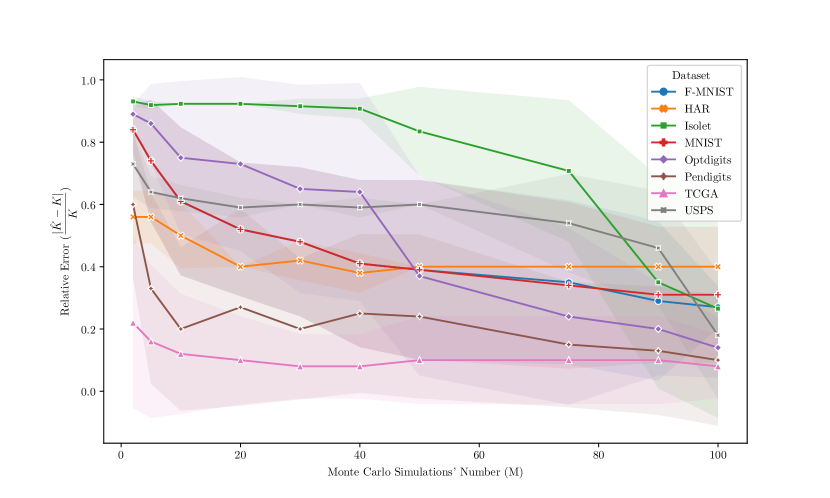
Figure 1: The plot illustrates the relative error between the estimated and actual values of the number of clusters $K$ generated by mp-means, as the number of Monte Carlo simulations increases. Each experiment was conducted over 10 executions, with the variance also depicted. The plot is more discernible in color.

4.2 Clustering Experiments

This section analyzes the performance of mp-means, an approach that incorporates mud-pod into the dip-means wrapper method, replacing dip-dist. This wrapper procedure begins with a single cluster and iteratively splits those clusters deemed by a multivariate unimodality test as likely having multiple subclusters. The procedure terminates when no further splits are suggested. A similar integration of the folding test yields the fold-means algorithm. In Table 3, we compare the performance of various clustering methods estimating the number of clusters across several datasets. It is important to note that in all our experiments, we use the raw flattened data encoding and apply only a feature-wise z-transformation. Although our method employs the Mahalanobis distance and is scale-agnostic, we observed that scaling profoundly affects other algorithms. Our experiments include datasets like USPS, MNIST, Fashion-MNIST (F-MNIST), Human Activity Recognition (HAR), Optdigits, Pendigits, Isolet, and TCGA. Detailed dataset descriptions are provided in Appendix A. As ground truth number of clusters, the number of classes was considered in all datasets. We benchmark against classic algorithms, including x-means (Pelleg & Moore, 2000), g-means (Pelleg & Moore, 2000), pg-means (Feng & Hamerly, 2006), dip-means (Kalogeratos & Likas, 2012), and hdbscan (Campello et al., 2013). A detailed overview of the algorithms and their hyperparameter setups are provided in Appendix B. Our evaluation metrics consist of the estimated number of clusters (k) and the Normalized Mutual Information (NMI). NMI values lie between [0, 1], where 1 signifies a perfect match and 0 represents an arbitrary result.

This experiment set, encompassing both the complexity of many modes and inherent clustering errors, is notably more challenging than single-class unimodality testing. We observe that most of the classical approaches, notably x-means and g-means, have the tendency to predict a high value for $k$, frequently estimating around 35 clusters for datasets such as USPS, MNIST, and F-MNIST. Similarly, x-means, for instance, consistently overestimates the $k$ value on these datasets, accompanied by NMI values which, while respectable, do not always achieve the top tier. In contrast, pg-means often significantly underestimates the number of clusters, suggesting a notable disparity in its clustering from the ground truth. This assertion is further supported by its suboptimal NMI values across multiple datasets, with values as low as 0.14 for the USPS dataset. Hdbscan demonstrates a varying range in $k$ values across datasets, highlighting its adaptability. However, this variability does not always correlate with high NMI values. Its performance on the USPS dataset, where it estimates 13 clusters with an NMI of 0.38, is a case in point.

Turning our attention to the HAR dataset, the dip-means and mp-means methods are particularly notable. They estimate $k$ values closely aligned with the ground truth of 5 and simultaneously achieve the highest NMI scores, specifically 0.73. This is indicative of their robustness and accuracy in deciphering the cluster structure inherent to the data. In the context of the Optdigits and Pendigits datasets, dip-means struggles to align its $k$ estimations with the ground truth, predicting values of 1 and 16, respectively. Conversely, mp-means appears more consistent, with $k$ values of 8 and 14 for Optdigits and Pendigits, respectively, and corresponding NMI scores that are commendable. In an experiment with k-means using accurate cluster count, the NMI of mp-means closely aligns with, or even exceeds, that of k-means. Finally, the projection dimension of mp-means varies between subclusters. The experiments underscore its robustness across multiple projection spaces. In conclusion, while various algorithms demonstrate strengths in certain areas, the consistent performance of mp-means across multiple datasets underscores its utility in solving clustering problems with unknown number of clusters.

Ablation Study on Simulations’ Number: In Figure 1, the relative error between the estimated number of clusters $K$ and the true value, as deduced by the mp-means algorithm, is depicted against the number of Monte Carlo simulations ($M$). The shaded regions around each line represent the variance over 10 executions, highlighting result consistency. As observed, for all datasets, an increase in the number of Monte Carlo simulations tends to correspond with a decline in the relative error, signifying an enhancement in the accuracy of $k$ estimation. While some datasets exhibit minimal spread, others display significant variance, suggesting the need for more Monte Carlo simulations. This suggests a need for more projections on certain datasets. However, as noted in the table, this variance does not significantly impede $k$ estimation. Summarizing, Figure 1 substantiates the notion that increasing the number of Monte Carlo simulations augments the precision of the mp-means algorithm’s cluster estimation, albeit with varying degrees of improvement across different datasets.

5 Conclusions

In this study, we addressed the challenges associated with generalizing the concept of unimodality testing to higher dimensions. Through the innovative integration of random projections and the notion of $\alpha$-unimodality, we have presented a novel methodology which offers a robust approach to multivariate unimodality testing. Leveraging both point-to-point distancing and linear random projections, our approach bridges the gap between the simplicity of one-dimensional unimodality confirmation and the intricacies of its higher-dimensional counterpart. By integrating our unimodality test with k-means, we introduced a new incremental clustering approach that automatically estimates the cluster count while performing clustering. Empirical evaluations underscored the efficacy of our test in both unimodality assessments and clustering scenarios, showcasing its indispensable applicability in diverse data-driven domains. Future exploration will focus to additional $\alpha$-unimodality preserving operations to enhance our test, experimenting with $\alpha$-unimodality for $\alpha\neq 1$, and applying the proposed test to other data analysis tasks, e.g., capturing covariate shift, time series change detection, etc.

Dataset	Type	Description	Size	Dimension	k	Source
USPS	Image	Handwritten digits	10000	256	10	Hull (1994)
MNIST	Image	Handwritten digits	10000	784	10	LeCun et al. (1998)
F-MNIST	Image	Zalando’s article image	10000	784	10	Xiao et al. (2017)
HAR	Time-series	Smartphone-based activity	2947	561	5	Kelly et al. (2023)
Optdigits	Image	Handwritten digits	1797	64	10	Kelly et al. (2023)
Pendigits	Time-series	Handwritten digits	10992	16	10	Kelly et al. (2023)
Isolet	Spectral	Speech recordings pronouncing letters	6238	617	26	Kelly et al. (2023)
TCGA	Tabular	Cancer gene expression profiles	801	20531	5	Kelly et al. (2023)

Table 4: Datasets for our experiments: Size indicates data instances, Dimension shows original encoding’s flattened size, and k represents ground-truth class labels.

Appendix A Clustering Datasets

Table 4 summarizes the benchmark datasets used in our experiments, varying in size, dimensions, number of classes $k$ (considered as ground-truth number of clusters), complexity, and domain. The datasets USPS, MNIST, and F-MNIST feature images of handwritten digits and fashion items, respectively. Specifically, USPS and MNIST contain grayscale images of handwritten digits from 0 to 9, with MNIST having a resolution of 28 x 28 pixels. In contrast, F-MNIST, or Fashion MNIST, encompasses grayscale images of ten clothing types, also at a resolution of 28 x 28 pixels. The Human Activity Recognition (HAR) dataset captures data from sensors to classify human activities, such as walking and sitting. OptDigits and Pendigits both pertain to handwritten digits: OptDigits consists of 8 x 8 resolution images, while Pendigits uses 16-dimensional vectors containing pixel coordinates. The Isolet dataset is an assemblage of speech recordings, representing the sounds of spoken letters, characterized by vectors with 617 spectral coefficients derived from the speech. Finally, TCGA is a compendium of gene expression profiles garnered from RNA sequencing of diverse cancer specimens, inclusive of clinical data, normalized counts, gene annotations, and pathways for five cancer types. For USPS, MNIST, and F-MNIST, we use the test datasets with 10000 points. For other datasets, we utilize the full set, typically containing fewer than 10000 points, except for Pendigits. Despite better preliminary results, we we constrained the sizes of USPS, MNIST, and F-MNIST to their test sets to avoid sample number bias.

Appendix B Clustering Algorithms

In this section, we provide an overview of the clustering algorithms employed in our experiments. We focus on methods that automatically estimate the number of clusters. We benchmark our approach against well-established algorithms, namely x-means (Pelleg & Moore, 2000), g-means (Pelleg & Moore, 2000), pg-means (Feng & Hamerly, 2006), dip-means (Kalogeratos & Likas, 2012), and hdbscan (Campello et al., 2013). Given our design’s adherence to the original dataspace, we exclude methods combining learning embeddings and clustering, like deep clustering approaches. To select the best number of clusters, x-means incorporates a regularization penalty guided by the Bayesian Information Criterion (BIC), which accounts for model complexity. However, this approach excels mainly with abundant data and distinct spherical clusters. Another extension, g-means, tests the assumption that each cluster originates from a Gaussian distribution. Given the challenges of statistical tests in high dimensions, g-means first projects cluster datapoints onto a high variance axis and then employs the Anderson-Darling test for normality. Clusters failing this test are iteratively split to identify the Gaussian mixture. Conversely, projected g-means (pg-means) assumes a Gaussian mixture for the entire dataset, evaluating the model as a whole. It relies on the EM algorithm, constructing one-dimensional projections of both the dataset and the learned model, and subsequently assessing model fit in the projected space using the Kolmogorov-Smirnov (KS) test. This approach’s strength lies in identifying overlapping Gaussian clusters of varying scales and covariances.

Moreover, hdbscan enhances dbscan by transforming it into a hierarchical clustering method and subsequently employs a technique to derive a flat clustering based on cluster stability. Hdbscan aims to obtain an optimal cluster solution by maximizing the aggregate stability of chosen clusters. Both mp-means and fold-means build upon the wrapper method (dip-means) introduced in the work of Kalogeratos & Likas (2012). Dip-means draws upon this approach and uses the dip-dist criterion internally. These methods incrementally increase cluster count and apply unimodality tests to clusters shaped by k-means. The process concludes when all clusters are characterized as unimodal.

For baseline model hyperparameters, we adopt a significance level $a=0.01$ for all relevant algorithms. The default setups are used for x-means and g-means from Novikov (2019), pg-means as per Feng & Hamerly (2006), and hdbscan following McInnes et al. (2017). The default hyperparameters for dip-means are those provided by the authors. For the folding test, we utilize the publicly available Python version. Given the folding test’s propensity to indicate multimodality, we set a cap on $k$ for fold-means. Specifically, for all algorithms necessitating a maximum $k$ value, we set $k_{\text{max}}=300$.

References

- Bhattacharya et al. (2009) Bhattacharya, A., Kar, P., and Pal, M. On low distortion embeddings of statistical distance measures into low dimensional spaces. In Bhowmick, S. S., Küng, J., and Wagner, R. (eds.), Database and Expert Systems Applications, pp. 164–172, Berlin, Heidelberg, 2009. Springer Berlin Heidelberg. ISBN 978-3-642-03573-9.
- Campello et al. (2013) Campello, R. J. G. B., Moulavi, D., and Sander, J. Density-based clustering based on hierarchical density estimates. In Pei, J., Tseng, V. S., Cao, L., Motoda, H., and Xu, G. (eds.), Advances in Knowledge Discovery and Data Mining, pp. 160–172, Berlin, Heidelberg, 2013. Springer Berlin Heidelberg. ISBN 978-3-642-37456-2.
- Chasani & Likas (2022) Chasani, P. and Likas, A. The uu-test for statistical modeling of unimodal data. Pattern Recognition, 122:108272, 2022. ISSN 0031-3203. doi: https://doi.org/10.1016/j.patcog.2021.108272. URL https://www.sciencedirect.com/science/article/pii/S0031320321004520.
- Dai (1989) Dai, T. On multivariate unimodal distributions, 1989. URL https://open.library.ubc.ca/collections/ubctheses/831/items/1.0097413.
- Dasgupta (1999) Dasgupta, S. Learning mixtures of gaussians. 40th Annual Symposium on Foundations of Computer Science (Cat. No.99CB37039), pp. 634–644, 1999. URL https://api.semanticscholar.org/CorpusID:8338511.
- Daskalakis et al. (2013) Daskalakis, C., Diakonikolas, I., Servedio, R. A., Valiant, G., and Valiant, P. Testing k-Modal Distributions: Optimal Algorithms via Reductions, pp. 1833–1852. 2013. doi: 10.1137/1.9781611973105.131. URL https://epubs.siam.org/doi/abs/10.1137/1.9781611973105.131.
- Daskalakis et al. (2014) Daskalakis, C., Diakonikolas, I., and Servedio, R. A. Learning -modal distributions via testing. Theory of Computing, 10(20):535–570, 2014. doi: 10.4086/toc.2014.v010a020. URL https://theoryofcomputing.org/articles/v010a020.
- Dharmadhikari & Joag-Dev (1988) Dharmadhikari, S. and Joag-Dev, K. Unimodality, convexity, and applications. Elsevier, 1988.
- Diaconis & Freedman (1984) Diaconis, P. and Freedman, D. Asymptotics of Graphical Projection Pursuit. The Annals of Statistics, 12(3):793 – 815, 1984. doi: 10.1214/aos/1176346703. URL https://doi.org/10.1214/aos/1176346703.
- Dümbgen et al. (2013) Dümbgen, L., Conte-Zerial, D., et al. On low-dimensional projections of high-dimensional distributions. In From Probability to Statistics and Back: High-Dimensional Models and Processes–A Festschrift in Honor of Jon A. Wellner, volume 9, pp. 91–105. Institute of Mathematical Statistics, 2013.
- Dunn et al. (2021) Dunn, R., Gangrade, A., Wasserman, L., and Ramdas, A. Universal inference meets random projections: a scalable test for log-concavity. arXiv preprint arXiv:2111.09254, 2021.
- Feng & Hamerly (2006) Feng, Y. and Hamerly, G. Pg-means: learning the number of clusters in data. In Schölkopf, B., Platt, J., and Hoffman, T. (eds.), Advances in Neural Information Processing Systems, volume 19. MIT Press, 2006. URL https://proceedings.neurips.cc/paper_files/paper/2006/file/a9986cb066812f440bc2bb6e3c13696c-Paper.pdf.
- Fernandez-Granda (2016) Fernandez-Granda, C. Random projections and compressed sensing. Lecture Notes in Optimization-based Data Analysis, 2016. URL https://cims.nyu.edu/~cfgranda/pages/OBDA_spring16/material/random_projections.pdf. New York University.
- Hartigan & Hartigan (1985) Hartigan, J. A. and Hartigan, P. M. The Dip Test of Unimodality. The Annals of Statistics, 13(1):70 – 84, 1985. doi: 10.1214/aos/1176346577. URL https://doi.org/10.1214/aos/1176346577.
- Hotelling (1931) Hotelling, H. The Generalization of Student’s Ratio. The Annals of Mathematical Statistics, 2(3):360 – 378, 1931. doi: 10.1214/aoms/1177732979. URL https://doi.org/10.1214/aoms/1177732979.
- Hull (1994) Hull, J. J. Database for handwritten text recognition research. In IEEE Transactions on pattern analysis and machine intelligence, volume 16, pp. 550–554. IEEE, 1994.
- Johnson & Lindenstraus (1984) Johnson, W. B. and Lindenstraus, J. Extensions of lipschitz mappings into hilbert space. Contemporary mathematics, 26:189–206, 1984.
- Kalogeratos & Likas (2012) Kalogeratos, A. and Likas, A. Dip-means: an incremental clustering method for estimating the number of clusters. In Pereira, F., Burges, C., Bottou, L., and Weinberger, K. (eds.), Advances in Neural Information Processing Systems, volume 25. Curran Associates, Inc., 2012. URL https://proceedings.neurips.cc/paper_files/paper/2012/file/a8240cb8235e9c493a0c30607586166c-Paper.pdf.
- Kelly et al. (2023) Kelly, M., Longjohn, R., and Nottingham, K. The uci machine learning repository, 2023. URL https://archive.ics.uci.edu/ml. Last accessed: October 31, 2023.
- Khintchine (1938) Khintchine, A. Y. On unimodal distributions. Izv. Nsuchno-Issled. Inst. Mat. Meh. Tomsk. Goa. Univ., 2:1–7, 1938. in Russian.
- Konstantellos (1980) Konstantellos, A. Unimodality conditions for gaussian sums. IEEE Transactions on Automatic Control, 25(4):838–839, 1980. doi: 10.1109/TAC.1980.1102410.
- LeCun et al. (1998) LeCun, Y., Bottou, L., Bengio, Y., and Haffner, P. Gradient-based learning applied to document recognition. Proceedings of the IEEE, 86(11):2278–2324, 1998.
- Lehmann & Romano (2005) Lehmann, E. L. and Romano, J. P. Testing statistical hypotheses. Springer Texts in Statistics. Springer, New York, third edition, 2005. ISBN 0-387-98864-5.
- Lopes et al. (2011) Lopes, M., Jacob, L., and Wainwright, M. J. A more powerful two-sample test in high dimensions using random projection. In Shawe-Taylor, J., Zemel, R., Bartlett, P., Pereira, F., and Weinberger, K. (eds.), Advances in Neural Information Processing Systems, volume 24. Curran Associates, Inc., 2011. URL https://proceedings.neurips.cc/paper_files/paper/2011/file/5487315b1286f907165907aa8fc96619-Paper.pdf.
- McInnes et al. (2017) McInnes, L., Healy, J., and Astels, S. hdbscan: Hierarchical density based clustering. The Journal of Open Source Software, 2(11):205, 2017.
- Novikov (2019) Novikov, A. PyClustering: Data mining library. Journal of Open Source Software, 4(36):1230, apr 2019. doi: 10.21105/joss.01230. URL https://doi.org/10.21105/joss.01230.
- Olshen & Savage (1970) Olshen, R. A. and Savage, L. J. A generalized unimodality. Journal of Applied Probability, 7(1):21–34, 1970. ISSN 00219002. URL http://www.jstor.org/stable/3212145.
- Pelleg & Moore (2000) Pelleg, D. and Moore, A. W. X-means: Extending k-means with efficient estimation of the number of clusters. In Proceedings of the Seventeenth International Conference on Machine Learning, ICML ’00, pp. 727–734, San Francisco, CA, USA, 2000. Morgan Kaufmann Publishers Inc. ISBN 1558607072.
- Radhendushka Srivastava & Ruppert (2016) Radhendushka Srivastava, P. L. and Ruppert, D. Raptt: An exact two-sample test in high dimensions using random projections. Journal of Computational and Graphical Statistics, 25(3):954–970, 2016. doi: 10.1080/10618600.2015.1062771. URL https://doi.org/10.1080/10618600.2015.1062771.
- Schubert (2023) Schubert, E. Stop using the elbow criterion for k-means and how to choose the number of clusters instead. SIGKDD Explor. Newsl., 25(1):36–42, jul 2023. ISSN 1931-0145. doi: 10.1145/3606274.3606278. URL https://doi.org/10.1145/3606274.3606278.
- Sharipov (2011) Sharipov, O. S. Glivenko-Cantelli Theorems, pp. 612–614. Springer Berlin Heidelberg, Berlin, Heidelberg, 2011. ISBN 978-3-642-04898-2. doi: 10.1007/978-3-642-04898-2˙280. URL https://doi.org/10.1007/978-3-642-04898-2_280.
- Siffer et al. (2018) Siffer, A., Fouque, P.-A., Termier, A., and Largouët, C. Are your data gathered? In Proceedings of the 24th ACM SIGKDD International Conference on Knowledge Discovery & Data Mining, KDD ’18, pp. 2210–2218, New York, NY, USA, 2018. Association for Computing Machinery. ISBN 9781450355520. doi: 10.1145/3219819.3219994. URL https://doi.org/10.1145/3219819.3219994.
- Silverman (1981) Silverman, B. W. Using kernel density estimates to investigate multimodality. Journal of the Royal Statistical Society. Series B (Methodological), 43(1):97–99, 1981. ISSN 00359246. URL http://www.jstor.org/stable/2985156.
- Xiao et al. (2017) Xiao, H., Rasul, K., and Vollgraf, R. Fashion-mnist: a novel image dataset for benchmarking machine learning algorithms, 2017.