Numerical Method for a Controlled Sweeping Process with Nonsmooth Sweeping Set

Abstract

The numerical method developed in verachadinum for optimal control problems involving sweeping processes with smooth sweeping set $C$ is generalized to the case where $C$ is nonsmooth, namely, $C$ is the intersection of a finite number of sublevel sets of smooth functions. The novelty of this extension resides in producing for the general setting a different approach, since the one used for the smooth sweeping sets is not applicable here.

1 Introduction

Sweeping processes refer to a specific category of differential inclusions that incorporates the normal cone to a set called sweeping set. This distinctive feature leads to differential inclusions that are unbounded and discontinuous. The initial appearance of such a model goes back to the papers moreau1 ; moreau2 ; moreau3 by J.J. Moreau in which he introduced this system as a framework for investigating the dynamics of plasticity and friction. Subsequently, various adaptations of this model have surfaced in a wide range of applications, including but not limited to engineering, mechanics, crowd motion problems, and economics, etc (see outrata and its references).

Over the past few years, extensive research has been conducted on optimal control problems over various versions of sweeping processes with particular focus on establishing the existence of optimal solutions and on deriving necessary optimality conditions, see e.g.,brokate ; ccmn ; ccmnbis ; cmo0 ; cmo ; cmo2 ; chhm2 ; chhm ; cmn0 ; henrion ; palladino ; pinho ; pinhoEr ; pinholast ; VCpaper ; verachadisvaa ; verachadijune ; verachadijca ; verachadi . However, numerical methods for such problems are quite limited in the literature, with a few notable exceptions given in outrata ; pinhonum ; verachadinum .

In this paper we are interested in constructing a numerical algorithm to solve a fixed time Mayer problem $(P)$ in which the dynamic is a controlled sweeping process $(D)$, the sweeping set $C$ is the intersection of the zero-sublevel sets of a finite sequence of functions $\psi_{i}\colon\mathbb{R}^{n}\longrightarrow\mathbb{R}$, $i=1,\dots,r$, and the initial state is a fixed point $x_{0}$ in $C$. This problem $(P)$ was successfully treated numerically in pinhonum for the special case: the initial state $x_{0}$ lies in the interior of $C$, and $C$ is convex and of class $\mathcal{C}^{2}$, that is, $r=1$ and $\psi:=\psi_{1}$ is convex and $\mathcal{C}^{2}$. The main idea used in pinhonum , which differs from that used in outrata , consists of approximating ($D$) by the system ($D_{\gamma_{k}}$), obtained by replacing in ($D$) the normal cone $N_{C}(x(t))$ by the penalty term $\gamma_{k}e^{\gamma_{k}\psi(x(t))}\nabla\psi(x(t))$. Then, the so obtained standard optimal control problem is solved numerically over piecewise constant controls. This numerical method is generalized in verachadinum to allow the initial state $x_{0}$ to be any point in $C$, including its boundary, and to nonconvex and $\mathcal{C}^{1,1}$ sweeping sets $C$. However, the smoothness of $C$ remains an essential assumption in verachadinum which naturally excludes a large class of nonsmooth sweeping sets arising from applications.

The goal of this paper is to expand the domain of applicability of the numerical method in verachadinum to a general form of $(P)$, namely, for $r>1$. In this case, $C$ is not necessarily smooth for being the intersection of the zero-sublevel sets of a finite sequence of $\mathcal{C}^{1,1}$-functions $\psi_{i}$, $i=1,\dots,r$. While transitioning from $r=1$ to $r>1$ might be initially perceived as a minor generalization, a close examination shows that this is not the case, since this transition actually necessitates a major overhaul of the approach used in verachadinum . This is due to the fact that when $r>1$, the set $C$ is the zero-sublevel of the function $\psi:=\max\{\psi_{i}:i=1,\dots,r\},$ which is only guaranteed to be Lipschitz, and hence, it renders the exponential penalization technique of verachadinum inapplicable. To circumvent this major obstacle, we approximate the nonsmooth max-function $\psi$ by a well constructed sequence $\psi_{\gamma_{k}}$ of $\mathcal{C}^{1,1}$ functions, and hence, we use in the definition of $(D_{\gamma_{k}})$ the exponential penalization technique for $\psi_{\gamma_{k}}$. It turns out that the so-obtained $(D_{\gamma_{k}})$ is equivalent to an approximating control system having $r$-penalty terms that involve $\nabla\psi_{i}$, $i=1,\dots,r$. However, having solved the nonsmoothness issue with $\psi$ by means of $\psi_{\gamma_{k}}$, we now encounter a new hurdle caused by the generalized Hessian of the sequence $(\psi_{\gamma_{k}})_{k}$ not being uniformly bounded. This issue requires new ideas that will be revealed when establishing, parallel to verachadinum , the theoretical results needed for the development of our numerical method.

The layout of the paper is as follows. In the next section, we present our basic notations and definitions, and we state our optimal control problem $(P)$ over a sweeping process. In Section 3, we list our hypotheses, and provide some preparatory results. In Section 4, we establish three theoretical results, namely, Propositions 6, 7 and 8, that form the backbone of the main result obtained in Section 5 as Theorem 5.1. This theorem confirms that optimal trajectories of well-constructed approximating problems converge to an optimal trajectory for the original problem $(P)$. This result leads to designing our proposed numerical algorithm in Section 5. The effectiveness of this algorithm is tested on a numerical example elaborated in Section 6. More precisely, using our algorithm we compute a numerical optimal trajectory for our example and we show that it is actually a good approximation of an exact optimal trajectory produced by means of the maximum principle established in verachadijca . The last section of the paper contains some concluding remarks.

2 Basic Notations and Definitions, and Statement of $(P)$

2.1 Basic Notations and Definitions

We denote by $\|\cdot\|$ and $\langle\cdot,\cdot\rangle$, the Euclidean norm and the usual inner product, respectively. The open and the closed unit balls are respectively denoted by $B$ and $\bar{B}$. For $x\in\mathbb{R}^{n}$ and $\rho\geq 0$, the open and the closed balls of radius $\rho$ centered at $x$ are respectively written as $B_{\rho}(x)$ and $\bar{B}_{\rho}(x)$. For a set $S\subset\mathbb{R}^{n}$, $\textnormal{int}\,S$, $\textnormal{bdry}\,S$, $\textnormal{cl}\,S$, $\textnormal{conv}\,S$, and $S^{c}$ designate the interior, the boundary, the closure, the convex hull, and the complement of $S$, respectively. The Lebesgue space of essentially bounded measurable functions $f\colon[a,b]\longrightarrow\mathbb{R}^{n}$ is denoted by $L^{\infty}([a,b];\mathbb{R}^{n})$. For the sets of absolutely continuous functions and of bounded variations functions $f\colon[a,b]\longrightarrow\mathbb{R}^{n}$ we use, respectively, $AC([a,b];\mathbb{R}^{n})$ and $BV([a,b];\mathbb{R}^{n})$. A function $f\colon\mathbb{R}^{n}\longrightarrow\mathbb{R}$ is $\mathcal{C}^{1,1}$ if it is Fréchet differentiable with locally Lipschitz derivative. A function $\pi\colon A\longrightarrow B$ is bi-Lipschitz if it is a Lipschitz bijection onto $B$, and its inverse is also Lipschitz.

Now we present some notations and definitions from Nonsmooth Analysis and Geometry. For standard references, see, e.g., the monographs brudnyi ; clarkeold ; clsw ; delfour ; mordubook ; rockwet ; ThibaultBook . Let $S$ be a nonempty and closed subset of $\mathbb{R}^{n}$, and let $s\in S$. The proximal, the Mordukhovich (also known as limiting), and the Clarke normal cones to $S$ at $s$ are denoted by $N^{P}_{S}(s)$, $N_{S}^{L}(s)$, and $N_{S}(s)$, respectively. For the Clarke tangent cone to $S$ at $s$, we use $T_{S}(s)$. The set $S$ is said to be epi-Lipschitz if for all $s\in S$, the Clarke normal cone of $S$ at $s$ is pointed, that is, $N_{S}(s)\cap-N_{S}(s)=\{0\}$. For $\rho>0$, the set $S$ is said to be $\rho$-prox-regular if for all $s\in S$ and for all unit vector $\zeta\in N_{S}^{P}(s)$, we have $\langle\zeta,x-s\rangle\leq\frac{1}{2\rho}\|x-s\|^{2}$ for all $x\in S$. This latter inequality is known as the proximal normal inequality. Finally, we say that $S$ is quasiconvex if there exists $c\geq 0$ such that any two points $s_{1},\hskip 0.42677pts_{2}$ in $S$ can be joined by a polygonal line $\gamma$ in $S$ satisfying $l(\gamma)\leq c\hskip 0.42677pt\|s_{1}-s_{2}\|,$ where $l(\gamma)$ denotes the length of $\gamma$.

2.2 Statement of $(P)$

This paper focuses on developing a numerical algorithm to solve the following fixed time Mayer problem

$$\begin{array}[]{l}(P)\colon\;\hbox{Minimize}\;g(x(T))\\ \hskip 25.6073pt\hbox{over}\;(x,u)\;\hbox{such that}\;u\in\mathscr{U},\;x\in AC([0,T];\mathbb{R}^{n}),\,\hbox{and}\\[2.0pt] \hskip 25.6073pt(D)\begin{cases}\dot{x}(t)\in f(x(t),u(t))-N_{C}(x(t)),\;\;\hbox{a.e.}\;t\in[0,T]\\ x(0)=x_{0},\end{cases}\end{array}$$

where $T>0$ is fixed, $g\colon\mathbb{R}^{n}\longrightarrow\mathbb{R}$, $f\colon\mathbb{R}^{n}\times\mathbb{R}^{m}\longrightarrow\mathbb{R}^{n}$, $C$ is the intersection of the zero-sublevel sets of a finite sequence of functions $\psi_{i}\colon\mathbb{R}^{n}\longrightarrow\mathbb{R}$, $i=1,\dots,r$, $N_{C}(\cdot)$ stands for the Clarke normal cone to $C$, $x_{0}\in C$ is fixed, and, for a given nonempty set $U\subset\mathbb{R}^{m}$, the set of control functions $\mathscr{U}$ is defined as

$$\mathscr{U}:=\left\{u\colon[0,T]\longrightarrow\mathbb{R}^{m}\;\;\hbox{is measurable and}\;\;u(t)\in U\;\;\hbox{a.e.}\;t\in[0,T]\right\}.$$

A pair $(x,u)$ is admissible for $(P)$ if $x\colon[0,T]\longrightarrow\mathbb{R}^{n}$ is absolutely continuous, $u\in\mathscr{U}$, and $(x,u)$ satisfies the controlled  sweeping process $(D)$ called the dynamic of $(P)$. An admissible pair $(\bar{x},\bar{u})$ for $(P)$ is said to be an optimal solution if $g(\bar{x}(T))\leq g(x(T))$ for all pairs $(x,u)$ admissible for $(P)$. In that case, $\bar{x}$ is called an optimal trajectory of $(P)$.

3 Hypotheses and Preparatory Results

3.1 Hypotheses

We assume throughout this paper that the data of $(P)$ satisfy the following hypotheses:

1. $f$ is continuous on $C\times U$; and there exists $M>0$ such that $x\mapsto f(x,u)$ is $M$-Lipschitz for all $u\in U$; and $\|f(x,u)\|\leq M$ for all $(x,u)\in C\times U.$

2. $f(x,U)$ is convex for all $x\in\mathbb{R}^{n}$, and $U$ is compact.

3. $C\not=\emptyset$ is given by

   $$C:=\bigcap_{i=1}^{r}C_{i},\;\hbox{where}\;C_{i}:=\{x\in\mathbb{R}^{n}:\psi_{i}(x)\leq 0\}\;\hbox{and}$$

   $(\psi_{i})_{1\leq i\leq r}$ is a family of $\mathcal{C}^{1,1}$ functions $\psi_{i}\colon\mathbb{R}^{n}\longrightarrow\mathbb{R}$. Moreover, for $i=1,\dots,r$, $C_{i}$ is compact, with $\textnormal{bdry}\,C_{i}$ connected for $n>1$ and $C_{i}$ is convex for $n=1$, and there is a constant $\eta>0$ such that

   $$\left\|\sum_{i\in\mathcal{I}^{0}_{c}}\lambda_{i}\nabla\psi_{i}(c)\right\|>2\eta,\;\;\forall c\in\{x\in\mathbb{R}^{n}:\mathcal{I}^{0}_{x}\not=\emptyset\},$$

   where $\mathcal{I}^{0}_{x}:=\{i\in\{1,\dots,r\}:\psi_{i}(x)=0\}$ and $(\lambda_{i})_{i\in\mathcal{I}^{0}_{c}}$ is any sequence of nonnegative numbers satisfying $\sum_{i\in\mathcal{I}^{0}_{c}}\lambda_{i}=1$.

4. $g$ is $L_{g}$-Lipschitz on $C$.

We denote by $\bar{M}_{\psi}$ a common upper bound over $C$ of the finite sequence $(\|\nabla\psi_{i}(\cdot)\|)_{i=1}^{r}$ such that $\bar{M}_{\psi}\geq 2\eta$, and by $2M_{\psi}$ a common Lipschitz constant of the finite family $\{\nabla\psi_{i}\}_{i=1}^{r}$ over the compact set $\textnormal{conv}\,C$. We also denote by:

1. $\psi\colon\mathbb{R}^{n}\longrightarrow\mathbb{R}$ the function defined by

   $$\psi(x):=\max\{\psi_{i}(x):i=1,\dots,r\},\;\;\forall x\in\mathbb{R}^{n}.$$

   Clearly we have that $C=\{x\in\mathbb{R}^{n}:\psi(x)\leq 0\}.$

2. $(\gamma_{k})_{k}$ a sequence satisfying $\gamma_{k}>\frac{2M}{\eta}$ for all $k\in\mathbb{N}$, with $\gamma_{k}\longrightarrow\infty\;\hbox{as}\;k\longrightarrow\infty$.

3. $(\alpha_{k})_{k}$ and $(\sigma_{k})_{k}$ the two real sequences defined by

   $$\alpha_{k}:=\frac{\ln\left(\frac{\eta\gamma_{k}}{2{M}}\right)}{\gamma_{k}}\;\,\hbox{and}\;\,\sigma_{k}:=\frac{r{M}_{\psi}}{2\eta^{2}}\bigg{(}\frac{\ln(r)}{\gamma_{k}}+\alpha_{k}\bigg{)},\;\;\;k\in\mathbb{N}.$$ (1)

   For $(\alpha_{k})_{k}$, we have $\gamma_{k}e^{-\alpha_{k}\gamma_{k}}=\frac{2{M}}{\eta},$ $\alpha_{k}>0$ for all $k\in\mathbb{N}$, and $\alpha_{k}\searrow 0$. For $(\sigma_{k})_{k}$, we have $\sigma_{k}>0$ for all $k\in\mathbb{N}$, and $\sigma_{k}\searrow 0$.

4. $(\psi_{\gamma_{k}})_{k}$ the sequence of functions $\psi_{\gamma_{k}}\colon\mathbb{R}^{n}\longrightarrow\mathbb{R}$ defined by

   $$\psi_{\gamma_{k}}(x):=\frac{1}{\gamma_{k}}\ln\Bigg{(}\sum_{i=1}^{r}e^{\gamma_{k}\psi_{i}(x)}\Bigg{)},\;\;\forall x\in\mathbb{R}^{n}.$$ (2)

   Clearly we have that

   $$\nabla\psi_{\gamma_{k}}(x)=\frac{\sum\limits_{i=1}^{r}e^{\gamma_{k}\psi_{i}(x)}\nabla\psi_{i}(x)}{\sum\limits_{i=1}^{r}e^{\gamma_{k}\psi_{i}(x)}},\;\;\forall x\in\mathbb{R}^{n}.$$ (3)

5. $(C_{i}(k))_{k}$ the sequence defined, for $i=1,\dots,r$, by

   $$C_{i}(k):=\{x\in\mathbb{R}^{n}:\psi_{i}(x)\leq-\alpha_{k}\}.$$

6. $(C^{\gamma_{k}})_{k}$ and $(C^{\gamma_{k}}(k))_{k}$ the two sequences defined by

   $$C^{\gamma_{k}}:=\{x\in\mathbb{R}^{n}:\psi_{\gamma_{k}}(x)\leq 0\}=\bigg{\{}x\in\mathbb{R}^{n}:\sum_{i=1}^{r}e^{\gamma_{k}\psi_{i}(x)}\leq 1\bigg{\}},\;\hbox{and}$$ (4)

   $$C^{\gamma_{k}}(k):=\{x\in\mathbb{R}^{n}:\psi_{\gamma_{k}}(x)\leq-\alpha_{k}\}=\bigg{\{}x\in\mathbb{R}^{n}:\sum_{i=1}^{r}e^{\gamma_{k}\psi_{i}(x)}\leq\frac{2{M}}{\eta\gamma_{k}}\bigg{\}}.$$ (5)

   One can easily see that if $r=1$, then $\psi_{\gamma_{k}}$, $C^{\gamma_{k}}$, and $C^{\gamma_{k}}(k)$ coincide with $\psi$, $C$, and $C(k):=\{x\in\mathbb{R}^{n}:\psi(x)\leq-\alpha_{k}\}$, respectively.

3.2 Preparatory Results

This subsection consists of preparatory results that are fundamental for the rest of the paper. Note that some of these results are extracted from the papers VCpaper ; verachadijca ; verachadi , and hence, their proofs are omitted here.

We begin with the following proposition which gives important properties of the set $C$.

Proposition 1 ((verachadijca, , Proposition 4.1))

The set $C$ is $\frac{\eta}{M_{\psi}}$-prox-regular, epi-Lipschitz with $C=\textnormal{cl}\,(\textnormal{int}\,C)$, and, for all $x\in\textnormal{bdry}\,C$ we have

$$N_{C}(x)=N^{P}_{C}(x)=N^{L}_{C}(x) = \bigcup_{\lambda\geq 0}\lambda\partial\psi(x)$$

$$= \Bigg{\{}\sum_{i\in\mathcal{I}_{x}^{0}}\lambda_{i}\nabla\psi_{i}(x):\lambda_{i}\geq 0\Bigg{\}}\not=\{0\}.$$

Moreover, we have

$$\textnormal{int}\,C=\bigcap_{i=1}^{r}\textnormal{int}\,C_{i}=\bigcap_{i=1}^{r}\{x\in\mathbb{R}^{n}:\psi_{i}(x)<0\}\not=\emptyset,\;\;\hbox{and}$$

$$\textnormal{bdry}\,C=C\cap\bigg{(}\bigcup_{i=1}^{r}\textnormal{bdry}\,C_{i}\bigg{)}\not=\emptyset.$$

For the sequence of functions $(\psi_{\gamma_{k}})_{k}$, we have the following.

Proposition 2 ((verachadijca, , Proposition 4.4))

The following assertions hold $:$

1. The sequence $(\psi_{\gamma_{k}})_{k}\in\mathcal{C}^{1,1}(\mathbb{R}^{n};\mathbb{R})$, is monotonically nonincreasing in $k$, and converges uniformly to $\psi$. Moreover, for all $k\in\mathbb{N}$ and for $i=1,\dots,r$, we have that

   $$\psi_{i}(x)\leq\psi(x)\leq\psi_{\gamma_{k}}(x)\leq\psi(x)+\frac{\ln(r)}{\gamma_{k}},\;\;\forall x\in\mathbb{R}^{n},\;and$$ (6)

   $$\|\nabla\psi_{\gamma_{k}}(x)\|\leq\bar{M}_{\psi},\;\;\forall x\in C.$$

2. There exist $k_{1}\in\mathbb{N}$ and $r_{1}>0$ such that for all $k\geq k_{1}$, for all $x\in\{x\in\mathbb{R}^{n}:\psi_{\gamma_{k}}(x)=0\}$, and for all $z\in B_{r_{1}}(x)$, we have

   $$\|\nabla\psi_{\gamma_{k}}(z)\|>2\eta.$$

   In particular, for $k\geq k_{1}$ we have

   $$[\psi_{\gamma_{k}}(x)=0]\Longrightarrow\|\nabla\psi_{\gamma_{k}}(x)\|>2\eta.$$ (7)

3. There exists $k_{2}\geq k_{1}$ and $\varepsilon_{o}>0$ such that for all $k\geq k_{2}$ we have

   $$\big{[}x\in C^{\gamma_{k}}\;\hbox{and}\;\|\nabla\psi_{\gamma_{k}}(x)\|\leq\eta\big{]}\implies\psi_{\gamma_{k}}(x)<-\varepsilon_{o}.$$

Remark 1

One can easily see from the definition of $\psi_{\gamma_{k}}$ in (2) that when $r>1$, the second inequality of (6) is strict, that is, $\psi_{i}(x)<\psi_{\gamma_{k}}(x)$ for all $x\in\mathbb{R}^{n}$ and for $i=1,\dots,r$. On the other hand, from (1)$(a)$, (5) and (6), we deduce that for all $k\in\mathbb{N}$ and for $i=1,\dots,r$, we have

$$\gamma_{k}e^{\gamma_{k}\psi_{i}(x)}\leq\gamma_{k}e^{\gamma_{k}\psi(x)}\leq\gamma_{k}e^{\gamma_{k}\psi_{\gamma_{k}}(x)}\leq\frac{2M}{\eta},\,\;\forall x\in C^{\gamma_{k}}(k).$$

Employing the preceding proposition and (verachadi, , Proposition 3.1), we show the following properties for the sequence of sets $(C^{\gamma_{k}})_{k}$. One novelty of this Proposition is provided in the second part of its item $(c)$, namely, that for $k$ large enough, the sets $C^{\gamma_{k}}$ are uniformly prox-regular with a uniform prox-regularity constant being $\frac{\eta}{2M_{\psi}}$. Note that in (verachadi, , Proposition 3.1) it is only established that $C^{\gamma_{k}}$ is $\frac{\eta}{M_{\psi_{\gamma_{k}}}}$-prox-regular, where $2M_{\psi_{\gamma_{k}}}$ depends on $k$, for being the Lipschitz constant of $\nabla\psi_{\gamma_{k}}$ over the compact set $\textnormal{conv}\,C$. Thus, establishing the uniform prox-regularity is not straightforward, since the generalized Hessian of $\psi_{\gamma_{k}}$ is unbounded and so is the sequence $(M_{\psi_{\gamma_{k}}})_{k}$.

Proposition 3

For all $k$, the set $C^{\gamma_{k}}\subset C$ is compact with $C^{\gamma_{k}}\subset\textnormal{int}\,C$ for $r>1$. Moreover, there exists $k_{3}\geq k_{2}$ such that for $k\geq k_{3}$, we have$\hskip 0.42677pt:$

1. $\textnormal{bdry}\,C^{\gamma_{k}}=\{x\in\mathbb{R}^{n}:\psi_{\gamma_{k}}(x)=0\}=\left\{x\in\mathbb{R}^{n}:\sum_{i=1}^{r}e^{\gamma_{k}\psi_{i}(x)}=1\right\}\not=\emptyset.$

2. $\textnormal{int}\,C^{\gamma_{k}}=\{x\in\mathbb{R}^{n}:\psi_{\gamma_{k}}(x)<0\}\not=\emptyset.$

3. $C^{\gamma_{k}}$ is epi-Lipschitzian, $C^{\gamma_{k}}=\textnormal{cl}\,(\textnormal{int}\,C^{\gamma_{k}})$, and $C^{\gamma_{k}}$ is $\frac{\eta}{2M_{\psi}}$-prox-regular.

4. For all $x\in\textnormal{bdry}\,C^{\gamma_{k}}$ we have

   $$N_{C^{\gamma_{k}}}(x)=N^{P}_{C^{\gamma_{k}}}(x)=N^{L}_{C^{\gamma_{k}}}(x) = \bigg{\{}\lambda\nabla\psi_{\gamma_{k}}(x):\lambda\geq 0\bigg{\}}$$

   $$= \bigg{\{}\lambda\sum\limits_{i=1}^{r}e^{\gamma_{k}\psi_{i}(x)}\nabla\psi_{i}(x):\lambda\geq 0\bigg{\}}.$$

Furthermore, the sequence $(C^{\gamma_{k}})_{k}$ is a nondecreasing sequence whose Painlevé-Kuratowski limit is $C$ and satisfies

$$\textnormal{int}\,C=\bigcup_{k\in\mathbb{N}}\textnormal{int}\,C^{\gamma_{k}}=\bigcup_{k\in\mathbb{N}}C^{\gamma_{k}}.$$ (8)

Proof From (6) and the definition of $C^{\gamma_{k}}$ in (4), we conclude that $C^{\gamma_{k}}\subset C$ for all $k$. This gives that the closed set $C^{\gamma_{k}}$ is bounded for all $k$, and hence $C^{\gamma_{k}}$ is compact for all $k$. On the other hand, for $r>1$, if $x\in C^{\gamma_{k}}$ then by (4), we have $\psi_{\gamma_{k}}(x)\leq 0,$ which yields that $\psi_{i}(x)<0$ for $i=1,\dots,r$, by Remark 1. Hence,

$$x\in\bigcap_{i=1}^{r}\textnormal{int}\,C_{i}=\textnormal{int}\,C.$$

Therefore, for $r>1$, we have $C^{\gamma_{k}}\subset\textnormal{int}\,C$ for all $k$.

As $\textnormal{int}\,C\not=\emptyset,$ then, for any $x\in\textnormal{int}\,C$ we have $x\in C$ and $\psi(x)<0.$ Using (6), there exists $k_{3}\geq k_{2}$, such that for $k\geq k_{3}$, we have that

$$\psi_{\gamma_{k}}(x)\leq\psi(x)+\frac{\ln(r)}{\gamma_{k}}<0.$$

This gives that $x\in C^{\gamma_{k}}$, and hence $C^{\gamma_{k}}\not=\emptyset$ for $k\geq k_{3}$. Note that both arguments made above yield that

$$\textnormal{int}\,C\subset\bigcup_{k\in\mathbb{N}}\textnormal{int}\,C^{\gamma_{k}}\subset\bigcup_{k\in\mathbb{N}}\textnormal{int}\,C^{\gamma_{k}}\subset\textnormal{int}\,C.$$

This gives that (8) holds true. Hence, since by Proposition 2, $\psi_{\gamma_{k}}$ is $C^{1,1}$ and satisfies (7), we deduce that all the properties satisfied by the set $C$ in (verachadi, , Proposition 3.1) are also satisfied by $C^{\gamma_{k}}$ for all $k\geq k_{2}$. Therefore, the assertions $(a)$-$(d)$ of Proposition 3 are valid except the uniform constant for the prox-regularity of $C^{\gamma_{k}}$. For, let $x\in\textnormal{bdry}\,C^{\gamma_{k}}$ and let $0\not=\zeta\in N^{P}_{C^{\gamma_{k}}}(x)$. Then we have, for some $\lambda>0$, that

$$\zeta=\lambda\sum\limits_{i=1}^{r}e^{\gamma_{k}\psi_{i}(x)}\nabla\psi_{i}(x)\;\;\hbox{and}\;\;\sum\limits_{i=1}^{r}e^{\gamma_{k}\psi_{i}(x)}=1.$$ (9)

For $y$ fixed in $C^{\gamma_{k}}$ and for $t\in(0,1]$, we have $x+t(y-x)\in\textnormal{conv}\,C^{\gamma_{k}}\subset\textnormal{conv}\,C$. Since $2M_{\psi}$ is a common Lipschitz constant of the finite family $\{\nabla\psi_{i}\}_{i=1}^{r}$, it follows that, for $i=1,\dots,r$,

$$\langle\nabla\psi_{i}(x+t(y-x))-\nabla\psi_{i}(x),y-x\rangle = \frac{1}{t}\langle\nabla\psi_{i}(x+t(y-x))-\nabla\psi_{i}(x),t(x-y)\rangle$$

$$\geq -2tM_{\psi}\|x-y\|^{2}.$$

Hence, using the mean value theorem, we have for $i=1,\dots,r$ the existence of $t^{i}_{y}\in(0,1)$ such that

$$0\geq\psi_{i}(y)-\psi_{i}(x) = \langle\nabla\psi_{i}(x+t^{i}_{y}(y-x)),y-x\rangle$$

$$\geq -2t^{i}_{y}M_{\psi}\|x-y\|^{2}+\langle\nabla\psi_{i}(x),y-x\rangle.$$

Whence, for $i=1,\dots,r,$

$$\langle\nabla\psi_{i}(x),y-x\rangle\leq 2t^{i}_{y}M_{\psi}\|y-x\|^{2}\leq 2M_{\psi}\|y-x\|^{2}.$$

Using (9), this gives that

$$\langle\zeta,y-x\rangle\leq 2\lambda M_{\psi}\|y-x\|^{2}.$$

Therefore, from (3), (7) and (9), we conclude that

$$\left\langle\frac{\zeta}{\|\zeta\|},y-x\right\rangle\leq\frac{2\lambda M_{\psi}}{\|\zeta\|}\|y-x\|^{2}=\frac{2\lambda M_{\psi}}{\lambda\|\nabla\psi_{\gamma_{k}}(x)\|}\|y-x\|^{2}\leq\frac{M_{\psi}}{\eta}\|y-x\|^{2}.$$

This terminates the proof of the $\frac{\eta}{2M_{\psi}}$-prox-regularity of $C^{\gamma_{k}}$.

We proceed to prove the “Furthermore” part of Proposition 3. Since $(\psi_{\gamma_{k}})_{k}$ is monotonically nonincreasing in $k$, we deduce that the sequence $(C^{\gamma_{k}})_{k}$ is a nondecreasing sequence. Hence, it is easy to show (see e.g., (rockwet, , Exercice 4.3)) that the Painlevé-Kuratowski limit of the sequence $(C^{\gamma_{k}})_{k}$ satisfies

$$\lim_{k\longrightarrow\infty}C^{\gamma_{k}}=\textnormal{cl}\,\Bigg{(}\bigcup_{k\in\mathbb{N}}C^{\gamma_{k}}\Bigg{)}.$$ (10)

Now, upon taking the closure of $\textnormal{int}\,C$ in the already established (8) and using from Proposition 1 that $C=\textnormal{cl}\,({\textnormal{int}\,C})$, equation (10) yields that the Painlevé-Kuratowski limit of the sequence $(C^{\gamma_{k}})_{k}$ is $C$. ∎

We proceed to present the properties of the sequence of sets $(C^{\gamma_{k}}(k))_{k}$. For $c\in\textnormal{bdry}\,C$, we denote by $d_{c}$ the nonzero vector $d_{c}:=\sum_{j\in\mathcal{I}^{0}_{c}}v_{j}(c)$, where for $j=1,\dots,r$, $v_{j}(c)$ is the unique projection of $-\nabla\psi_{j}(c)$ to the Clarke tangent cone $T_{C}(c)$. For more information about the vector $d_{c}$, see (verachadijca, , Lemma 6.1). Note that when $r=1$, the vector $d_{c}$ coincides with $-\nabla\psi_{j}(c)\in T_{C}(c)$.

Proposition 4 ((verachadijca, , Proposition 4.3 & Remark 4.4))

The following assertions hold $:$

1. For all $k$, the set $C^{\gamma_{k}}(k)\subset\textnormal{int}\,C^{\gamma_{k}}\subset\textnormal{int}\,C$ and is compact. Moreover, there exists $k_{4}\geq k_{3}$ such that for $k\geq k_{4}$, we have$\hskip 0.42677pt:$

   1. $\textnormal{bdry}\,C^{\gamma_{k}}(k)=\{x\in\mathbb{R}^{n}:\psi_{\gamma_{k}}(x)=-\alpha_{k}\}\\ \hskip 52.63777pt=\left\{x\in\mathbb{R}^{n}:\sum_{i=1}^{r}e^{\gamma_{k}\psi_{i}(x)}=\frac{2{M}}{\eta\gamma_{k}}\right\}\not=\emptyset.$

   2. $\textnormal{int}\,C^{\gamma_{k}}(k)=\{x\in\mathbb{R}^{n}:\psi_{\gamma_{k}}(x)<-\alpha_{k}\}\not=\emptyset.$

   3. $[\psi_{\gamma_{k}}(x)=-\alpha_{k}]\Longrightarrow\|\nabla\psi_{\gamma_{k}}(x)\|>\eta.$

   4. $C^{\gamma_{k}}(k)$ is $\frac{\eta}{4M_{\psi}}$-prox-regular, and epi-Lipschitz with

      $$C^{\gamma_{k}}(k)=\textnormal{cl}\,(\textnormal{int}\,C^{\gamma_{k}}(k)).$$

   5. For all $x\in\textnormal{bdry}\,C^{\gamma_{k}}(k)$ we have

      $$N_{C^{\gamma_{k}}(k)}(x)=N^{P}_{C^{\gamma_{k}}(k)}(x) = N^{L}_{C^{\gamma_{k}}(k)}(x))$$

      $$= \bigg{\{}\lambda\nabla\psi_{\gamma_{k}}(x):\lambda\geq 0\bigg{\}}$$

      $$= \bigg{\{}\lambda\sum\limits_{i=1}^{r}e^{\gamma_{k}\psi_{i}(x)}\nabla\psi_{i}(x):\lambda\geq 0\bigg{\}}.$$

2. The sequence $(C^{\gamma_{k}}(k))_{k}$ is a nondecreasing sequence whose Painlevé-Kuratowski limit is $C$ and satisfies

   $$\textnormal{int}\,C=\bigcup_{k\in\mathbb{N}}\textnormal{int}\,C^{\gamma_{k}}(k)=\bigcup_{k\in\mathbb{N}}C^{\gamma_{k}}(k).$$ (11)

3. For $c\in\textnormal{bdry}\,C$, there exist ${k}_{c}\geq k_{4}$ and ${r}_{c}>0$ such that

   $$\left(\left[C\cap\bar{B}_{{r}_{c}}({c})\right]+\sigma_{k}\frac{d_{c}}{\|d_{c}\|}\right)\subset\textnormal{int}\,C^{\gamma_{k}}(k)\subset\textnormal{int}\,C^{\gamma_{k}},\;\;\forall k\geq{k}_{c}.$$

   In particular, for $k\geq{k}_{c}$ we have

   $$\left({c}+\sigma_{k}\frac{d_{c}}{\|d_{c}\|}\right)\in\textnormal{int}\,C^{\gamma_{k}}(k)\subset\textnormal{int}\,C^{\gamma_{k}}.$$

For $x_{0}$ the initial point of the problem $(P)$, we define the sequence $\left(x_{0}^{k}\right)_{k}$ by

$$x_{0}^{k}:=\begin{cases}x_{0},\;\forall k\in\mathbb{N},&\;\hbox{if}\;x_{0}\in\textnormal{int}\,{C},\vspace{0.2cm}\\ \displaystyle{x_{0}}+\sigma_{k}\frac{d_{x_{0}}}{\|d_{x_{0}}\|},\;\forall k\in\mathbb{N},&\;\hbox{if}\;x_{0}\in\textnormal{bdry}\,C.\end{cases}$$ (12)

Since $\sigma_{k}\longrightarrow 0$, the following lemma follows from (11) and Proposition 4$(iii)$.

Lemma 1

The sequence $x_{0}^{k}$ converges to $x_{0}$, and there exists $k_{5}\geq k_{x_{0}}$ such that $x_{0}^{k}\in C^{\gamma_{k}}(k)$ for all $k\geq k_{5}$.

Remark 2

From (H3) we can deduce that for $i=1,\dots,r$, the set $C_{i}$ satisfies the same assumptions satisfied by $C$ in the papers VCpaper ; verachadinum ; verachadi . Hence, all the properties established in those papers for $C$ and $C(k)$ are valid here for $C_{i}$ and $C_{i}(k)$, respectively, where $i=1,\dots,r$. On the other hand, from (6) and Remark 1, we have

$$C^{\gamma_{k}}(k)\subset\bigcap_{i=1}^{r}C_{i}(k),$$ (13)

and when $r>1$, $C_{i}(k)$ can be replaced in (13) by $\textnormal{int}\,C_{i}(k)$.

We terminate this section with the following proposition in which we provide properties of the projection maps from $\textnormal{bdry}\,C$ to $\textnormal{bdry}\,C^{\gamma_{k}}(k)$ and from $\textnormal{bdry}\,C^{\gamma_{k}}$ to $\textnormal{bdry}\,C^{\gamma_{k}}(k)$.

Proposition 5

There exists $k_{6}\geq k_{5}$ such that for $k\geq k_{6}$, the projection map $\pi_{k}\colon\textnormal{bdry}\,C\longrightarrow\textnormal{bdry}\,C^{\gamma_{k}}(k)$ is onto and 2-Lipschitz, and the projection map $\hat{\pi}_{k}\colon\textnormal{bdry}\,C^{\gamma_{k}}\longrightarrow\textnormal{bdry}\,C^{\gamma_{k}}(k)$ is bi-Lipschitz.

Proof We begin with the projection map $\pi_{k}$. Since $C$ is compact, and, by Proposition 4, $C$ is the Painlevé-Kuratowski limit of $C^{\gamma_{k}}(k)$, we deduce that $d_{H}(C,C^{\gamma_{k}}(k))\longrightarrow 0$ as $k\longrightarrow 0$. This gives that, for $k$ sufficiently large, $d(c,{\textnormal{bdry}\,C^{\gamma_{k}}}(k))<\frac{\eta}{4M_{\psi}}$ for all $c\in\textnormal{bdry}\,C$. In addition, by Proposition 4$(d)$, we have that $C^{\gamma_{k}}(k)$ is $\frac{\eta}{4M_{\psi}}$-prox-regular for $k$ large enough. We conclude that, for $k$ sufficiently large, $\pi_{k}$ is a single valued function. Now, by taking $k$ large enough so that $d(c,{\textnormal{bdry}\,C^{\gamma_{k}}}(k))<\frac{\eta}{8M_{\psi}}$ for all $c\in\textnormal{bdry}\,C$, we deduce from (prox, , Theorem 4.8) that $\pi_{k}$ is 2-Lipschitz. We claim that ${k}$ can be taken large enough so that $\pi_{k}$ is an onto function. Indeed, due to the $\frac{\eta}{4M_{\psi}}$-prox-regularity of $C^{\gamma_{k}}(k)$, it is sufficient to prove that for $k$ large enough, we have for each $c\in\textnormal{bdry}\,C^{\gamma_{k}}(k)$,

$$(\textnormal{bdry}\,C)\cap\left[c,c+\frac{\eta}{4M_{\psi}}\frac{\nabla\psi_{\gamma_{k}}({c})}{\|\nabla\psi_{\gamma_{k}}({c})\|}\right)\not=\emptyset.$$

If not, then there exist an increasing sequence $k_{n}\in\mathbb{N}$ and a sequence $c_{n}\in\textnormal{bdry}\,C^{\gamma_{k_{n}}}(k_{n})$ such that

$$(\textnormal{bdry}\,C)\cap\left[c_{n},c_{n}+\frac{\eta}{4M_{\psi}}\frac{\nabla\psi_{\gamma_{k_{n}}}({c_{n}})}{\|\nabla\psi_{\gamma_{k_{n}}}({c_{n}})\|}\right)=\emptyset.$$

This gives that

$$\psi_{\gamma_{k_{n}}}(c_{n})=-\alpha_{k_{n}}\;\,\hbox{and}\;\,\psi\left(c_{n}+\frac{\eta}{8M_{\psi}}\frac{\nabla\psi_{\gamma_{k_{n}}}({c_{n}})}{\|\nabla\psi_{\gamma_{k_{n}}}({c_{n}})\|}\right)<0,\;\;\forall n.$$

Using the compactness of $C$, the convergence of $\alpha_{k_{n}}$ to $0$, and the inequalities of (6), it follows that there exist a subsequence of $k_{n}$, we do not relabel, a $\bar{c}\in C$, and a unit vector $\bar{v}$, such that

$$c_{n}\longrightarrow\bar{c}\in\textnormal{bdry}\,C,\;\,\frac{\nabla\psi_{\gamma_{k_{n}}}({c_{n}})}{\|\nabla\psi_{\gamma_{k_{n}}}({c_{n}})\|}\longrightarrow\bar{v},\;\,\hbox{and}\;\,\psi\left(\bar{c}+\frac{\eta}{8M_{\psi}}\bar{v}\right)\leq 0.$$

Hence,

$$\bar{c}+\frac{\eta}{8M_{\psi}}\bar{v}\in C.$$ (14)

Since each point in $\textnormal{bdry}\,C$ is the limit of a sequence of points in $C^{\gamma_{k_{n}}}(k_{n})$, then, the $\frac{\eta}{4M_{\psi}}$-prox-regularity of $C^{\gamma_{k_{n}}}(k_{n})$ implies that $\bar{v}\in N_{C}^{P}(\bar{c})$. Thus, the $\frac{\eta}{M_{\psi}}$-prox-regularity of $C$ yields that

$$\bar{c}+\frac{\eta}{8M_{\psi}}\bar{v}\in B_{\frac{\eta}{M_{\psi}}}\left(\bar{c}+\frac{\eta}{M_{\psi}}\bar{v}\right)\subset C^{c},$$

which contradicts (14).

We proceed to prove that $\hat{\pi}_{k}$ is bi-Lipschitz. By Proposition 3, the function $\psi_{\gamma_{k}}$ satisfies the same assumptions satisfied by the function $\psi$ in VCpaper . In addition, the two sets $C^{\gamma_{k}}$ and $C^{\gamma_{k}}(k)$ are defined in terms of $\psi_{\gamma_{k}}$ in the same way $C$ and $C(k)$ of VCpaper were defined in terms of $\psi$. Hence, from (VCpaper, , Theorem 3.1$(vi)$), we can deduce that, for $k$ large enough, $\hat{\pi}_{k}$ is bi-Lipschitz. ∎

Remark 3

Unlike the case $r=1$ studied in (VCpaper, , Theorem 3.1$(vi)$) and (verachadinum, , Lemma 2), the projection $\hat{\pi}_{k}$ here for $r>1$ cannot be shown to be uniformly bi-Lipschitz. The reason is that, when $r>1$, the generalized Hessian of the function $\psi_{\gamma_{k}}$ is not uniformly bounded. More issues surface for the projection ${\pi}_{k}$, since the function $\psi$ is only Lipschitz. These facts render the techniques used in the proof of (VCpaper, , Theorem 3.1$(vi)$) not applicable for either projections.

4 Key Results

Parallel to (verachadinum, , Section III), we provide in this section three theoretical results, that are the keystone of our numerical algorithm constructed for $(P)$. We note that having $\psi$ only Lipschitz and the generalized Hessian of $\psi_{\gamma_{k}}$ not bounded in the general case $r>1$, make the proofs of these results more challenging than their counterparts for the case $r=1$, and hence, new ideas and techniques are required.

For $x^{k}_{0}$ given in (12), we denote by $(D_{\gamma_{k}})$ the approximation dynamic defined by

$$({D}_{\gamma_{k}})\begin{cases}\dot{x}(t)=f(x(t),u(t))-\sum\limits_{i=1}^{r}\gamma_{k}e^{\gamma_{k}\psi_{i}(x(t))}\nabla\psi_{i}(x(t)),\;\textnormal{a.e.}\;t\in[0,T],\\ x(0)=x^{k}_{0}.\end{cases}$$ (15)

One can easily verify that using (3), the system $(D_{\gamma_{k}})$ can be rewritten in terms of $\psi_{\gamma_{k}}$ as follows:

$$({D}_{\gamma_{k}})\begin{cases}\dot{x}(t)=f(x(t),u(t))-\gamma_{k}e^{\gamma_{k}\psi_{\gamma_{k}}(x(t))}\nabla\psi_{\gamma_{k}}(x(t)),\;\textnormal{a.e.}\;t\in[0,T],\\ x(0)=x_{0}^{k}.\end{cases}$$ (16)

For a solution $x_{\gamma_{k}}$ of $(D_{\gamma_{k}})$ corresponding to a control $u\in\mathscr{U}$, we denote by $\xi_{\gamma_{k}}(\cdot)$ the sequence of non-negative continuous functions on $[0,T]$ defined by

$$\xi_{\gamma_{k}}(\cdot):=\gamma_{k}e^{\gamma_{k}\psi_{\gamma_{k}}(x_{\gamma_{k}}(\cdot))}\overset{\eqref{psigkdef}}{=}\sum_{i=1}^{r}\xi_{\gamma_{k}}^{i}(\cdot),$$

where $\xi_{\gamma_{k}}^{i}(\cdot):=\gamma_{k}e^{\gamma_{k}\psi_{i}(x_{\gamma_{k}}(\cdot))}$ for $i=1,\dots,r$.

From (verachadijca, , Theorem 4.13), we can deduce the following proposition.

Proposition 6

There exists $k_{7}\geq k_{6}$ such that for all $k\geq k_{7}$ and for all $u\in U$, the solution $x_{\gamma_{k}}$ of $(D_{\gamma_{k}})$ corresponding to $u$ satisfies $:$

1. $x_{\gamma_{k}}(t)\in C^{\gamma_{k}}(k)\subset\textnormal{int}\,C^{\gamma_{k}}\subset\textnormal{int}\,C$ for all $t\in[0,T]$.

2. $0<\xi_{\gamma_{k}}^{i}(t)\leq\xi_{\gamma_{k}}(t)\leq\frac{2{M}}{\eta}$ for all $t\in[0,T]$ and for $i=1,\dots,r.$

3. $\|\dot{x}_{\gamma_{k}}(t)\|\leq{M}+\frac{2{M}\bar{M}_{\psi}}{\eta}$  for a.e. $t\in[0,T]$.

In the following proposition, we prove that the $L^{\infty}$-distance between the solution $x_{\gamma_{k}}$ of $(D_{\gamma_{k}})$ and the solution $x$ of $(D)$ is controlled by $\sigma_{k}$, when the same control $u\in\mathscr{U}$ is used in both dynamics. Note that this result cannot be deduced from (verachadinum, , Proposition 2), where the function $\psi$ is replaced by our function $\psi_{\gamma_{k}}$. The reason behind this is that unlike the case for $\psi$ in (verachadinum, , Proposition 2), the Lipschitz constant for $\nabla\psi_{\gamma_{k}}$ is not uniformly bounded for $k$ large.

Proposition 7

There exists $k_{8}\geq k_{7}$ such that for all $k\geq k_{8}$ and for all $u\in\mathscr{U}$, the solution $x$ of system $(D)$ and the solution $x_{\gamma_{k}}$ of system $(D_{\gamma_{k}})$, both corresponding to the same control $u\in\mathscr{U}$, satisfy

$$\|x_{\gamma_{k}}(t)-x(t)\|^{2}\leq e^{\tilde{M}T}\sigma_{k}^{2}+\frac{8\eta M(e^{\tilde{M}T}-1)}{\tilde{M}M_{\psi}}\sigma_{k},\;\,\forall t\in[0,T]\;\textnormal{a.e.},$$

where $\tilde{M}:=\frac{5MM_{\psi}}{\eta}+2{M}$.

Proof As the Lipschitz constant of $\nabla\psi_{\gamma_{k}}$ is not uniformly bounded in $k$, a modification of the proof of (verachadinum, , Proposition 2) is required here. For this, we shall use the version (15) of $(D_{\gamma_{k}})$ instead of that in (16). Now, given that for $i=1,\dots,r$, $\psi_{i}$ is $\mathcal{C}^{1,1}$, the second-order generalized Taylor expansion, (hiriart, , Theorem 2.3), implies that for $x$ and $y$ in $C$, there exist $z_{i}\in\textnormal{conv}\,(C)$ and $M_{z_{i}}\in\partial^{2}\psi_{i}(z_{i})$ such that for $i=1,\dots,r$,

$$\psi_{i}(y)=\psi_{i}(x)+\langle\nabla\psi_{i}(x),y-x\rangle+\frac{1}{2}\langle M_{z_{i}}(y-x),y-x\rangle.$$

Hence, using that for $i=1,\dots,r$, $\|M_{z_{i}}\|\leq 2M_{\psi}$ and $\psi_{i}(y)\leq 0$, we obtain that for all $x$ and $y$ in $C$,

$$-\langle\nabla\psi_{i}(x),x-y\rangle\leq-\psi_{i}(x)+M_{\psi}\|x-y\|^{2}\;\;\hbox{for}\;i=1,\dots,r,$$ (17)

Employing (H1), (17), the inclusion of $(D)$, the prox-regularity of $C$, the version (15) of $(D_{\gamma_{k}})$, Lemma 1, and the uniform boundedness of $(\xi^{i}_{\gamma_{k}})_{i=1}^{r}$ in Proposition 1, we obtain that, for $k\geq k_{7}$ and for a.e. $t\in[0,T]$,

$$\frac{d}{dt}\|x_{\gamma_{k}}(t)-x(t)\|^{2}=2\langle x_{\gamma_{k}}(t)-x(t),\dot{x}_{\gamma_{k}}(t)-\dot{x}(t)\rangle$$ (18)

$$= 2\langle x_{\gamma_{k}}(t)-x(t),f(x(t),u(t))-\dot{x}(t)\rangle$$

$$+ 2\langle x_{\gamma_{k}}(t)-x(t),f(x_{\gamma_{k}}(t),u(t))-f(x(t),u(t))\rangle$$

$$- 2\sum_{i=1}^{r}\xi^{i}_{\gamma_{k}}(t)\langle x_{\gamma_{k}}(t)-x(t),\nabla\psi_{i}(x_{\gamma_{k}}(t))\rangle$$

$$\leq \frac{MM_{\psi}}{\eta}\left\|x_{\gamma_{k}}(t)-x(t)\right\|^{2}+2M\left\|x_{\gamma_{k}}(t)-x(t)\right\|^{2}$$

$$- 2\sum_{i=1}^{r}\xi^{i}_{\gamma_{k}}(t)\psi_{i}(x_{\gamma_{k}}(t))+2M_{\psi}\left\|x_{\gamma_{k}}(t)-x(t)\right\|^{2}\sum_{i=1}^{r}\xi^{i}_{\gamma_{k}}(t)$$

$$\leq \frac{MM_{\psi}}{\eta}\left\|x_{\gamma_{k}}(t)-x(t)\right\|^{2}+2M\left\|x_{\gamma_{k}}(t)-x(t)\right\|^{2}$$

$$- 2\sum_{i=1}^{r}\xi^{i}_{\gamma_{k}}(t)\psi_{i}(x_{\gamma_{k}}(t))+\frac{4MM_{\psi}}{\eta}\left\|x_{\gamma_{k}}(t)-x(t)\right\|^{2}$$

$$= \tilde{M}\left\|x_{\gamma_{k}}(t)-x(t)\right\|^{2}-2\sum_{i=1}^{r}\xi^{i}_{\gamma_{k}}(t)\psi_{i}(x_{\gamma_{k}}(t)),$$

where $\tilde{M}=\frac{5MM_{\psi}}{\eta}+2M$. Choose $k_{8}\geq k_{7}$ sufficiently large, so that $\gamma_{k}\geq\frac{2Me}{\eta}$ for all $k\geq k_{8}.$ This means that $a:=\frac{2M}{\eta\gamma_{k}}=e^{-\gamma_{k}\alpha_{k}}\leq e^{-1}$ for all $k\geq k_{8}$. Then, using the facts that $xa^{x}\leq a$ for $a\leq e^{-1}$ and $x\geq 1$, and that $\psi_{i}(x_{\gamma_{k}}(t))\leq\psi(x_{\gamma_{k}}(t))\leq\psi_{\gamma_{k}}(x_{\gamma_{k}}(t))\leq-\alpha_{k}$ for $i=1,\dots,r$ and for all $k\geq{k}_{8}$, we deduce with the help of (1)$(a)$ that for $i=1,\dots,r$,

$$-\xi^{i}_{\gamma_{k}}(t)\psi_{i}(x_{\gamma_{k}}(t)) = (\alpha_{k}\gamma_{k})\left(\frac{2M}{\eta\gamma_{k}}\right)^{\left(\frac{-\psi_{i}(x_{\gamma_{k}}(t))}{\alpha_{k}}\right)}\left(\frac{-\psi_{i}(x_{\gamma_{k}}(t))}{\alpha_{k}}\right)$$

$$\leq (\alpha_{k}\gamma_{k})\,\frac{2M}{\eta\gamma_{k}}=\frac{2M\alpha_{k}}{\eta},\quad\forall\hskip 0.42677ptt\in[0,T],\;\;\forall\hskip 0.42677ptk\geq{k}_{1}.$$

Hence by (18) we conclude that for $k\geq k_{8}$ and for a.e. $t\in[0,T]$

$$\frac{d}{dt}\|x_{\gamma_{k}}(t)-x(t)\|^{2}\leq\tilde{M}\left\|x_{\gamma_{k}}(t)-x(t)\right\|^{2}+\frac{4rM\alpha_{k}}{\eta}.$$

Now using Gronwall’s lemma (clsw, , Proposition 4.1.4), the definition of $\sigma_{k}$ in (1), and (12), we get that for $k\geq{k}_{8}$ and for all $t\in[0,T]$,

$$\|x_{\gamma_{k}}(t)-x(t)\|^{2} \leq e^{\tilde{M}T}\|x_{0}^{k}-x_{0}\|^{2}+\frac{4rM(e^{\tilde{M}T}-1)}{\eta\tilde{M}}\alpha_{k}$$

$$\leq e^{\tilde{M}T}\sigma_{k}^{2}+\frac{4r{M}(e^{\tilde{M}T}-1)}{\eta\tilde{M}}\alpha_{k}$$

$$\leq e^{\tilde{M}T}\sigma_{k}^{2}+\frac{8\eta M(e^{\tilde{M}T}-1)}{\tilde{M}M_{\psi}}\sigma_{k}.$$

This terminates the proof of the proposition. ∎

The following lemma is a generalization to the case when $r>1$ of (verachadinum, , Lemma 2), established for $r=1$, and hence, our $C^{\gamma_{k}}(k)$ here reduces to $C(k)$ there. Note that the proof of (verachadinum, , Lemma 2) is based on the uniform bi-Lipschitz continuity of the projection map from $\textnormal{bdry}\,C$ to $\textnormal{bdry}\,C(k)$; a property not met here for the projection map from $\textnormal{bdry}\,C$ to $\textnormal{bdry}\,C^{\gamma_{k}}(k)$, see Remark 3. Therefore, new ideas are needed here in order to prove this lemma. One may believe that this result could be established by replacing $C$ with $C^{\gamma_{k}}$ in that projection, that is, to use the projection map $\hat{\pi}_{k}$ from $\textnormal{bdry}\,C^{\gamma_{k}}$ to $\textnormal{bdry}\,C^{\gamma_{k}}(k)$. But, as mentioned in Remark 3, this projection map is not necessarily uniformly bi-Lipschitz. Moreover, the quasiconvexity required in the proof of (verachadinum, , Lemma 2) for $\textnormal{bdry}\,C$, is not guaranteed to be uniform here for $\textnormal{bdry}\,C^{\gamma_{k}}.$

Lemma 2

There exist $k_{9}\geq k_{8}$ and $\beta>0$ such that for all $k\geq k_{9}$,

$$\langle\nabla e^{\gamma_{k}\psi_{\gamma_{k}}(y)}-\nabla e^{\gamma_{k}\psi_{\gamma_{k}}(x)},y-x\rangle\geq-\frac{4r\beta MM_{\psi}}{\eta}\|y-x\|^{2},\;\,\forall x,\hskip 0.42677pty\in C^{\gamma_{k}}(k).$$

Proof From (verachadinum, , Lemma 2) applied to each $C_{i}$ for $i=1,\dots,r$, we get the existence of $k^{i}_{9}\geq k_{8}$ and $\beta_{i}>0$ such that for all $k\geq k^{i}_{9}$

$$\langle\nabla e^{\gamma_{k}\psi_{i}(y)}-\nabla e^{\gamma_{k}\psi_{i}(x)},y-x\rangle\geq-\frac{4\beta_{i}MM_{\psi}}{\eta}\|y-x\|^{2},\;\,\forall x,\hskip 0.42677pty\in C_{i}(k).$$

Using that $e^{\gamma_{k}\psi_{\gamma_{k}}(\cdot)}=\sum_{i=1}^{r}e^{\gamma_{k}\psi_{i}(\cdot)}$ and the inclusion (13), we conclude that for $k_{9}:=\max\{k_{9}^{i}:i=1,\dots,r\}$ and $\beta:=\max\{\beta_{i}:i=1,\dots,r\}$, we have for all $k\geq k_{9}$,

$$\langle\nabla e^{\gamma_{k}\psi_{\gamma_{k}}(y)}-\nabla e^{\gamma_{k}\psi_{\gamma_{k}}(x)},y-x\rangle\geq-\frac{4r\beta MM_{\psi}}{\eta}\|y-x\|^{2},\;\,\forall x,\hskip 0.42677pty\in C^{\gamma_{k}}(k).$$

The proof of the lemma is terminated.∎

Remark 4

When for all $i=1,\dots,r$, the set $C_{i}$ is convex (that is, $\psi_{i}$ is convex), then the result of Lemma 2 becomes straightforward since in that case the function $\psi_{\gamma_{k}}$ is convex, see (LiFang, , Lemma 3), which gives that $e^{\gamma_{k}\psi_{\gamma_{k}}(\cdot)}$ is convex, and hence,

$$\langle\nabla e^{\gamma_{k}\psi_{\gamma_{k}}(y)}-\nabla e^{\gamma_{k}\psi_{\gamma_{k}}(x)},y-x\rangle\geq 0,\;\,\forall x,\hskip 0.42677pty\in\mathbb{R}^{n}.$$

Note that for $n>1$, the convexity of $C_{i}$ implies that $\textnormal{bdry}\,C_{i}$ is connected.

Let $N$ be a positive integer and set $h:=\frac{T}{N}$. For any vector $\big{(}u_{1}^{N},\dots,u_{N}^{N})$ in $U^{N}:=\underbrace{U\times\cdots\times U}_{N}$, we associate the piecewise constant control function

$$u^{N}(t)\equiv u_{j}^{N}\;\,\hbox{for}\;\,t\in[(j-1)h,jh)\;\,\hbox{and}\;j=1,\dots,N.$$

We denote by $\mathscr{U}^{N}$ the set of such controls, and by $x^{N}_{\gamma_{k}}$ the solution of $(D_{\gamma_{k}})$ corresponding to a control $u^{N}\in\mathscr{U}^{N}$.

As in (verachadinum, , Section III), Lemma 2 leads to the following proposition, whose proof follows arguments similar to those used in the proof of (verachadinum, , Proposition 3).

Proposition 8

Let $u\in\mathscr{U}$ and, for $k\geq{k}_{9}$, let $x_{\gamma_{k}}$ be the solution of $(D_{\gamma_{k}})$ corresponding to $u$. Then there exists $u^{N}\in\mathscr{U}^{N}$ such that $x^{N}_{\gamma_{k}}$, the solution of $(D_{\gamma_{k}})$ corresponding to $u^{N},$ satisfies for $\delta_{j}:=\|x_{\gamma_{k}}(jh)-x^{N}_{\gamma_{k}}(jh)\|^{2}$ the inequality

$$\delta_{j}\leq\frac{2\hat{M}^{2}e^{6\bar{M}T}}{3\bar{M}}(1+6\bar{M}h)(1+\bar{M}h)h,\,\;\;\hbox{for}\;\,j=1,\dots,N,$$

where $\bar{M}:=M+\frac{4r\beta MM_{\psi}}{\eta}$ and $\hat{M}:={M}+\frac{2{M}\bar{M}_{\psi}}{\eta}.$

5 Numerical Algorithm

Based on the three key results of the previous section, namely Propositions 6, 7 and 8, we prove in this section the main result of this paper which inspires the construction of our numerical algorithm that solves $(P)$. We denote by $(P_{\gamma_{k}})$ the problem $(P)$ in which the dynamic $(D)$ is replaced by $(D_{\gamma_{k}})$, that is,

$$\begin{array}[]{l}(P_{\gamma_{k}})\colon\;\hbox{Minimize}\;g(x(T))\\ \hskip 33.28966pt\hbox{over}\;(x,u)\;\hbox{such that}\;u\in\mathscr{U},x\in AC([0,T];\mathbb{R}^{n}),\;\hbox{and}\\[2.0pt] \hskip 33.28966pt({D}_{\gamma_{k}})\begin{cases}\dot{x}(t)=f(x(t),u(t))-\gamma_{k}e^{\gamma_{k}\psi_{\gamma_{k}}(x(t))}\nabla\psi_{\gamma_{k}}(x(t)),\,\;\textnormal{a.e.}\;t\in[0,T],\\ x(0)=x_{0}^{k}.\end{cases}\end{array}$$

We fix $\varepsilon>0$. From Propositions 7 and 8, we have the following:

1. Since $\sigma_{k}\longrightarrow 0$ in Proposition 7, then, there exists $k_{\varepsilon}\geq k_{9}$ such that for a given solution $(\bar{x},\bar{u})$ of $(P)$ and for $\bar{x}_{\gamma_{k}}$ being the solution of $(D_{\gamma_{k}})$ corresponding to $\bar{u}$, we have

   $$\|\bar{x}-\bar{x}_{\gamma_{k}}\|_{\infty}\leq\frac{\varepsilon}{3L_{g}},\;\;\;\forall k\geq k_{\varepsilon}.$$

2. From Proposition 8, we deduce the existence of a positive integer $N_{\varepsilon}$ such that for $N\geq N_{\varepsilon}$ and $h:=\frac{T}{N}$, there is $\bar{u}^{N}\in\mathscr{U}^{N}$ for which the solution $\bar{x}^{N}_{\gamma_{k}}$ of $(D_{\gamma_{k}})$ corresponding to $\bar{u}^{N}$ satisfies

   $$\|\bar{x}_{\gamma_{k}}-\bar{x}_{\gamma_{k}}^{N}\|_{\infty}\leq\frac{\varepsilon}{3L_{g}},\;\;\;\forall k\geq k_{\varepsilon},\;\,\forall N\geq N_{\varepsilon}.$$

3. Let $N\geq N_{\varepsilon}$ and let $h:=\frac{T}{N}$. We denote by $\big{(}P_{\gamma_{k}}^{N}\big{)}$ the problem $(P_{\gamma_{k}})$ in which the controls are now restricted to $\mathscr{U}^{N}$, that is,

   $$\begin{array}[]{l}\big{(}P_{\gamma_{k}}^{N}\big{)}\colon\;\hbox{Minimize}\;g(x(T))\\[1.0pt] \hskip 34.71239pt\hbox{over}\;(x,u^{N})\in AC([0,T];\mathbb{R}^{n})\times\mathscr{U}^{N}\;\hbox{such that for}\;j=1,\dots,N,\\[1.0pt] \hskip 34.71239ptx(\cdot):=x^{j}(\cdot)\;\hbox{on}\,[(j-1)h,jh]\;\hbox{and}\;x^{j}\;\hbox{satisfies on}\;[(j-1)h,jh)\\[3.0pt] \hskip 34.14322pt\begin{cases}\dot{x}^{j}(t)=f(x^{j}(t),u^{N}_{j})-\gamma_{k}e^{\gamma_{k}\psi_{\gamma_{k}}(x^{j}(t))}\nabla\psi_{\gamma_{k}}(x^{j}(t)),\\[7.0pt] x^{j}((j-1)h)=\left[\begin{array}[]{@{}l@{\quad}l@{}}x_{0}^{k}&\hbox{if}\;j=1,\\[2.0pt] x^{j-1}((j-1)h)&\hbox{if}\;j\geq 2.\end{array}\right.\end{cases}\end{array}$$

   The compactness of $U^{N}$ yields that $\big{(}P_{\gamma_{k}}^{N}\big{)}$ admits an optimal solution. Denote by $\left(\hat{x}_{\gamma_{k}}^{N},\hat{u}_{\gamma_{k}}^{N}\right)$ one of the optimal solutions of $\big{(}P_{\gamma_{k}}^{N}\big{)}$ and by $\tilde{x}^{N}_{\gamma_{k}}$ the solution of $(D)$ corresponding to $\hat{u}_{\gamma_{k}}^{N}$. Then, by Proposition 7, we have that

   $$\|\hat{x}^{N}_{\gamma_{k}}-\tilde{x}_{\gamma_{k}}^{N}\|_{\infty}\leq\frac{\varepsilon}{3L_{g}},\;\;\;\forall k\geq k_{\varepsilon},\;\,\forall N\geq N_{\varepsilon}.$$

The following theorem, Theorem 5.1, is the culmination of all the results of this paper. It basically says that $\big{(}P_{\gamma_{k}}^{N}\big{)}$ approximates $(P)$ as $N\longrightarrow\infty$ and $k\longrightarrow\infty$. It extends (verachadinum, , Theorem 1 $\&$ Remark 4.1) to our general case, that is, when $C$ is the intersection of a finite number of sublevel sets of smooth functions. Since the statements of our Propositions 6, 7 and 8 here for the case $r>1$ are, respectively, similar to (verachadinum, , Propositions 1, 2 and 3), where $r=1$, then, the proof of Theorem 5.1 follows using arguments similar to those used in the proof of (verachadinum, , Theorem 1 $\&$ Remark 4.1).

Theorem 5.1

For $k\geq k_{\varepsilon}$ and $N\geq N_{\varepsilon}$, we have

$$g(\bar{x}(T))\leq g(\tilde{x}^{N}_{\gamma_{k}}(T))\leq g(\bar{x}(T))+\varepsilon,\;\;\hbox{and}$$

$$g(\bar{x}(T))-\frac{\varepsilon}{3}\leq g(\hat{x}^{N}_{\gamma_{k}}(T))\leq g(\bar{x}(T))+\frac{2\varepsilon}{3}.$$

Moreover, there exists an optimal solution $(\hat{x},\hat{u})$ of $(P)$ such that, up to a subsequence, both sequences $\hat{x}^{N}_{\gamma_{k}}$ and $\tilde{x}^{N}_{\gamma_{k}}$ converge uniformly to $\hat{x}$ as $N\longrightarrow\infty$ and $k\longrightarrow\infty$.

As a consequence of Theorem 5.1, we have the following Algorithm 1 that solves numerically the problem $(P)$.

Input: Positive integer $N$, numbers $\varepsilon>0$, $\gamma>0$ and $\delta>0$

Output: $\blacktriangleright$ Approximating minimum value of $(P)$
$\blacktriangleright$ Numerical optimal trajectory of $(P)$

1 Initialization;

2 $k\leftarrow 1$;

3 for $i\leftarrow 0$ to $1$ by $1$ do

4       $\gamma_{i}\leftarrow\gamma+i\hskip 0.42677pt\delta$;

5       compute $x_{0}^{i}$;

6       compute a solution $\hat{x}^{N}_{\gamma_{i}}$ of $\big{(}P_{\gamma_{i}}^{N}\big{)}$ for $\gamma_{i}$ and $x_{0}^{i}$;

7       $g_{i}\leftarrow g\big{(}\hat{x}^{N}_{\gamma_{i}}(T)\big{)}$;

8      

9 end for

10 while $|g_{k}-g_{k-1}|>\varepsilon$ do

11       $k\leftarrow k+1$;

12       $\gamma_{k}\leftarrow\gamma_{k-1}+\delta$;

13       compute $x_{0}^{k}$;

14       compute a solution $\hat{x}^{N}_{\gamma_{k}}$ of $\big{(}P_{\gamma_{k}}^{N}\big{)}$ for $\gamma_{k}$ and $x_{0}^{k}$;

15       $g_{k}\leftarrow g\big{(}\hat{x}^{N}_{\gamma_{k}}(T)\big{)}$;

16      

17 end while

return $g_{k}$;

Algorithm 1 Numerical Method for solving $(P)$

6 Example

To test our algorithm, we provide in this section an example of $(P)$ for which we separately calculate (i) an exact optimal solution using the Pontryagin-type maximum principle of verachadijca , and (ii) a numerical optimal trajectory using Algorithm 1. Then, we compare our answers.

We consider the following as data for the problem $(P)$:

1. The perturbation mapping $f\colon\mathbb{R}^{3}\times\mathbb{R}^{2}\longrightarrow\mathbb{R}^{3}$ is defined by

   $$f((x_{1},x_{2},x_{3}),(u,v)):=(x_{1}-2+u-v,4x_{2}+x_{3}+u+v,-x_{2}+4x_{3}+u+v).$$

2. The two functions $\psi_{1},\;\psi_{2}\colon\mathbb{R}^{3}\longrightarrow\mathbb{R}$ are defined by:

   1. $\psi_{1}(x_{1},x_{2},x_{3}):=(x_{1}-4)^{2}+x_{2}^{2}+x_{3}^{2}-25,$ and

   2. $\psi_{2}(x_{1},x_{2},x_{3}):=(x_{1}+4)^{2}+x_{2}^{2}+x_{3}^{2}-25.$

   Hence, the set $C=C_{1}\cap C_{2}$ is the intersection of the two solid spheres:

   1. $C_{1}=\{(x_{1},x_{2},x_{3}):(x_{1}-4)^{2}+x_{2}^{2}+x_{3}^{2}\leq 25\}$, and

   2. $C_{2}=\{(x_{1},x_{2},x_{3}):(x_{1}+4)^{2}+x_{2}^{2}+x_{3}^{2}\leq 25\}$.

   Note that $C$ is a nonsmooth and convex set, see Fig. 1.

   

   Figure 1: The sweeping set $C$ of Example 6

3. The objective function $g\colon\mathbb{R}^{3}\longrightarrow\mathbb{R}$ is defined by

   $$g(x_{1},x_{2},x_{3}):=x_{1}^{2}-x_{2}^{2}+|x_{3}|.$$

4. The control set is $U:=[-1,1]\times[-1,1]$, $T:=\tfrac{\pi}{2}$, and the initial point is $x_{0}:=(0,0,3)$.

One can easily verify that the hypotheses (H1)-(H4), and hence the assumptions (A1)-(A2.2) and (A2.4)-(A6) of verachadijca , are satisfied with $M=35$ and $\eta=2$. Moreover, we have $M_{\psi}=1$ and $\bar{M}_{\psi}=10$.

6.1 Exact optimal solution

In this subsection, we apply the Pontryagin-type maximum principle (verachadijca, , Theorem 3.1) to the problem $(P)$ of our example in order to find one of its optimal solution. Define the curve

$$\Gamma:=\{(x_{1},x_{2},x_{3}):x_{2}^{2}+x_{3}^{2}=9\;\hbox{and}\;x_{1}=0\}=(\textnormal{bdry}\,C_{1}\cap\textnormal{bdry}\,C_{2})\subset\textnormal{bdry}\,C.$$

Since $x_{0}\subset\Gamma$ and $g=-x_{2}^{2}+|x_{3}|$ on $\Gamma$ and is strictly greater than $-x^{2}_{2}+|x_{3}|$ elsewhere in $C$, we may seek for $(P)$ a candidate $(\bar{x},(\bar{u},\bar{v}))$ for optimality with $\bar{x}:=(\bar{x}_{1},\bar{x}_{2},\bar{x}_{3})$ belonging to $\Gamma$, if possible, and hence we have

$$\begin{cases}\bar{x}_{2}^{2}(t)+\bar{x}_{3}^{2}(t)=9\;\,\hbox{and}\,\;\bar{x}_{1}(t)=0,\;\,\forall t\in[0,\tfrac{\pi}{2}]\,\;\hbox{and}\\[1.0pt] \bar{x}(0)^{\mkern-1.5mu\mathsf{T}}=(0,0,3)\,\;\hbox{and}\;\,\bar{x}(\tfrac{\pi}{2})^{\mkern-1.5mu\mathsf{T}}=(0,\pm 3,0).\end{cases}$$ (19)

Note that the assumption (A2.3) of verachadijca is satisfied on $\Gamma$ for $\beta=(1,1)$. Then, applying (verachadijca, , Theorem 3.1) to such candidate $(\bar{x},(\bar{u},\bar{v}))$, we obtain the existence of an adjoint vector $p:=(p_{1},p_{2},p_{3})\in BV([0,\frac{\pi}{2}];\mathbb{R}^{3})$, two finite signed Radon measures $\nu_{1}$, $\nu_{2}$ on $\left[0,\frac{\pi}{2}\right]$, and $\xi_{1}$, $\xi_{2}\in L^{\infty}([0,\tfrac{\pi}{2}];\mathbb{R}^{+})$, such that when incorporating equations (19) into (verachadijca, , Theorem 3.1$(i)$-$(vi)$), we obtain the following:

1. The admissibility equation holds, that is, for $t\in[0,\tfrac{\pi}{2}]$ a.e.,

   $$\begin{cases}0=-2+\bar{u}(t)-\bar{v}(t)+8\xi_{1}(t)-8\xi_{2}(t),\\ \dot{\bar{x}}_{2}(t)=4\bar{x}_{2}(t)+\bar{x}_{3}(t)+\bar{u}(t)+\bar{v}(t)-2\bar{x}_{2}(t)(\xi_{1}(t)+\xi_{2}(t)),\\ \dot{\bar{x}}_{3}(t)=-\bar{x}_{2}(t)+4\bar{x}_{3}(t)+\bar{u}(t)+\bar{v}(t)-2\bar{x}_{3}(t)(\xi_{1}(t)+\xi_{2}(t)).\end{cases}$$

2. The adjoint equation is satisfied, that is, for $t\in[0,\frac{\pi}{2}]$,

   $$dp(t) = \begin{pmatrix}\begin{array}[]{rrr}-1&0&0\\ 0&-4&1\\ 0&-1&-4\end{array}\end{pmatrix}p(t)\hskip 0.42677ptdt\hskip 0.42677pt+\hskip 0.42677pt(\xi_{1}(t)+\xi_{2}(t))\begin{pmatrix}2\;\;&0\;\;&0\\ 0\;\;&2\;\;&0\\ 0\;\;&0\;\;&2\end{pmatrix}p(t)\hskip 0.42677ptdt\hskip 0.42677pt$$

   $$+ \hskip 0.42677pt\begin{pmatrix}-8\\ 2\bar{x}_{2}(t)\\ 2\bar{x}_{3}(t)\end{pmatrix}d\nu_{1}+\begin{pmatrix}8\\ 2\bar{x}_{2}(t)\\ 2\bar{x}_{3}(t)\end{pmatrix}d\nu_{2}.$$

3. The complementary slackness condition is valid, that is, for $t\in[0,\tfrac{\pi}{2}]$ a.e.,

   $$\begin{cases}\xi_{1}(t)(p_{2}(t)\bar{x}_{2}(t)+p_{3}(t)\bar{x}_{3}(t))=0,\\ \xi_{2}(t)(p_{2}(t)\bar{x}_{2}(t)+p_{3}(t)\bar{x}_{3}(t))=0.\end{cases}$$

4. The transversality condition holds, that is,

   $$p(\tfrac{\pi}{2})^{\mkern-1.5mu\mathsf{T}}\in\{(0,\pm 6,\alpha):\alpha\in[-1,1]\}.$$

5. 1. $\max\limits_{u\in[-1,1]}\{u\hskip 0.42677pt(p_{1}(t)+p_{2}(t)+p_{3}(t))\}$ is attained at $\bar{u}(t)$ for $t\in[0,\frac{\pi}{2}]$ a.e.

   2. $\max\limits_{v\in[-1,1]}\{v\hskip 0.42677pt(-p_{1}(t)+p_{2}(t)+p_{3}(t))\}$ is attained at $\bar{v}(t)$ for $t\in[0,\frac{\pi}{2}]$ a.e.

We temporarily assume that

$$\begin{cases}p_{1}(t)+p_{2}(t)+p_{3}(t)\geq 0,\,\;\forall t\in[0,\tfrac{\pi}{2}]\;\hbox{a.e.},\;\hbox{and}\\ -p_{1}(t)+p_{2}(t)+p_{3}(t)\leq 0,\,\;\forall t\in[0,\tfrac{\pi}{2}]\;\hbox{a.e.}\end{cases}$$ (20)

This gives from (e) that $\bar{u}(t)=1$ and $\bar{v}(t)=-1$ for $t\in[0,\frac{\pi}{2}]$ a.e. Now solving the differential equations of (a) and using (19), we obtain that

$$\xi_{1}(t)=\xi_{2}(t)=1\;\,\hbox{and}\;\,\bar{x}(t)^{\mkern-1.5mu\mathsf{T}}=(0,3\sin t,3\cos t),\;\;\forall t\in[0,\tfrac{\pi}{2}].$$

Hence, from (c) and (d), we deduce that

$$\begin{cases}p(\tfrac{\pi}{2})^{\mkern-1.5mu\mathsf{T}}\in\{(0,6,\alpha):\alpha\in[-1,1]\},\;\hbox{and}\\ p_{2}(t)\sin t+p_{3}(t)\cos t=0,\;\,\forall t\in[0,\tfrac{\pi}{2}]\;\textnormal{a.e.}\end{cases}$$ (21)

Moreover, the adjoint equation (b) simplifies to the following

$$\begin{cases}d{p}_{1}(t)=3p_{1}(t)\hskip 0.42677ptdt-8(d\nu_{1}-d\nu_{2}),\\ dp_{2}(t)=p_{3}(t)\hskip 0.42677ptdt+6(d\nu_{1}+d\nu_{2})\sin t,\\ d{{p}}_{3}(t)=-p_{2}(t)\hskip 0.42677ptdt+6(d\nu_{1}+d\nu_{2})\cos t.\end{cases}$$ (22)

Using (21) and (22), a simple calculation gives that

$$\begin{cases}p(\tfrac{\pi}{2})^{\mkern-1.5mu\mathsf{T}}=(0,6,-1)\;\;\hbox{and}\;\;p(t)^{\mkern-1.5mu\mathsf{T}}=(e^{3t},\cos t,-\sin t)\;\hbox{on}\;[0,\tfrac{\pi}{2}),\\ \;d\nu_{1}=\tfrac{1}{2}\Big{(}1+\tfrac{e^{\frac{3\pi}{2}}}{8}\Big{)}\delta_{\left\{\frac{\pi}{2}\right\}}\;\;\hbox{and}\;\;d\nu_{2}=\tfrac{1}{2}\Big{(}1-\tfrac{e^{\frac{3\pi}{2}}}{8}\Big{)}\delta_{\left\{\frac{\pi}{2}\right\}}\;\hbox{on}\;[0,\tfrac{\pi}{2}].\end{cases}$$

where $\delta_{\{a\}}$ denotes the unit measure concentrated on the point $a$. Note that for all $t\in[0,\tfrac{\pi}{2})$, we have $p_{1}(t)+p_{2}(t)+p_{3}(t)\geq 0$ and $-p_{1}(t)+p_{2}(t)+p_{3}(t)\leq 0$, and hence, the temporary assumption (20) is satisfied.

Therefore, the above analysis, realized via (verachadijca, , Theorem 3.1), produces an admissible pair $(\bar{x},(\bar{u},\bar{v}))$, where

$$\bar{x}(t)^{\mkern-1.5mu\mathsf{T}}=(0,3\sin t,3\cos t)\;\;\hbox{and}\;\;\bar{u}(t)=-\bar{v}(t)=1,\;\;\forall t\in[0,\tfrac{\pi}{2}],$$

which is optimal for $(P)$. This yields that

$$\min\,(P)=g(0,3,0)=-9.$$ (23)

6.2 Numerical optimal trajectory

The goal of this subsection is to test the effectiveness of Algorithm 1. Using our algorithm, We numerically compute estimates for both the minimum value and for an optimal trajectory of $\big{(}P_{\gamma_{k}}^{N}\big{)}$ of our example. Then, we verify that these computed estimations are in fact good approximations, respectively, for the exact minimum value and for the exact optimal trajectory of $(P)$ calculated in Subsection 6.1. This confirms the statement of Theorem 5.1.

We begin by calculating the vector $d_{x_{0}}$, where $x_{0}=(0,0,3)$. Clearly we have $\mathcal{I}^{0}_{x_{0}}=\{1,2\}$, and hence, $d_{x_{0}}:=v_{1}(x_{0})+v_{2}(x_{0})$, where $v_{1}(x_{0})$ and $v_{2}(x_{0})$ are the projections of $-\nabla\psi_{1}(x_{0})$ and $-\nabla\psi_{2}(x_{0})$ to $T_{C}(x_{0})$, respectively. We calculate $N_{C}(x_{0})$ and $T_{C}(x_{0})$, so we find

$$N_{C}(x_{0}) = \{\lambda_{1}\nabla\psi_{1}(x_{0})+\lambda_{2}\nabla\psi_{2}(x_{0}):\lambda_{1}\geq 0\;\hbox{and}\;\lambda_{2}\geq 0\}$$

$$= \{\lambda_{1}(-8,,0,6)+\lambda_{2}(8,0,6):\lambda_{1}\geq 0\;\hbox{and}\;\lambda_{2}\geq 0\},\;\hbox{and}$$

$$T_{C}(x_{0})=\{(x_{1},x_{2},x_{3}):[3x_{3}\leq-4x_{1}\;\hbox{and}\;x_{1}\geq 0]\;\hbox{or}\;[3x_{3}\leq 4x_{1}\;\hbox{and}\;x_{1}\leq 0]\}.$$

Then, the projection of $-\nabla\psi_{1}(x_{0})=(8,0,-6)$ and $-\nabla\psi_{2}(x_{0})=(-8,0,-6)$ to $T_{C}(x_{0})$ are $\left(\tfrac{144}{25},0,-\tfrac{192}{25}\right)$ and $\left(-\tfrac{144}{25},0,-\tfrac{192}{25}\right)$, respectively. This yields that,

$$d_{x_{0}}=\left(\tfrac{144}{25},0,-\tfrac{192}{25}\right)+\left(-\tfrac{144}{25},0,-\tfrac{192}{25}\right)=\left(0,0,-\tfrac{384}{25}\right).$$

Therefore,

$$\frac{d_{x_{0}}}{\|d_{x_{0}}\|}=(0,0,-1).$$ (24)

Now, having $M=35$, $\eta=2$ and $M_{\psi}=1$, we deduce from (1), (12) and (24) that for all $k$,

$$x_{0}^{k}=\left(0,0,3-\tfrac{\ln(2\gamma_{k})-\ln 35}{4\gamma_{k}}\right).$$

We proceed and we write explicitly the problem $\left(P_{\gamma_{k}}^{N}\right)$ corresponding to $(P)$.

$$\begin{array}[]{l}\big{(}P_{\gamma_{k}}^{N}\big{)}\colon\hbox{Minimize}\;x^{N}(\frac{\pi}{2})^{2}-y^{N}(\tfrac{\pi}{2})^{2}+|z^{N}(\tfrac{\pi}{2})|,\vspace{0.1cm}\\ \hskip 31.2982pt\hbox{over}\;((u^{1},v^{1}),\dots,(u^{N},v^{N}))\in([-1,1]\times[-1,1])^{N}\vspace{0.1cm}\\ \hskip 31.2982pt\hbox{such that for}\;j=1,\dots,N,\;\hbox{we have on}\;\left[(j-1)\frac{\pi}{2N},j\frac{\pi}{2N}\right)\vspace{0.1cm}\\ \hskip 27.03003pt\begin{cases}\dot{x}^{j}=x^{j}-2+u^{j}-v^{j}-2\xi^{1}_{\gamma_{k}}(x^{j}-4)-2\xi^{2}_{\gamma_{k}}(x^{j}+4),\\[2.0pt] \dot{y}^{j}=z^{j}+4y^{j}+u^{j}+v^{j}-2\xi^{1}_{\gamma_{k}}y^{j}-2\xi^{2}_{\gamma_{k}}y^{j},\\[2.0pt] \dot{z}^{j}=-y^{j}+4z^{j}+u^{j}+v^{j}-2\xi^{1}_{\gamma_{k}}z^{j}-2\xi^{2}_{\gamma_{k}}z^{j},\\[2.5pt] \xi^{1}_{\gamma_{k}}=\gamma_{k}e^{\gamma_{k}((x^{j}-4)^{2}+(y^{j})^{2})+(z^{j})^{2}-25)},\\[2.0pt] \xi^{2}_{\gamma_{k}}=\gamma_{k}e^{\gamma_{k}((x^{j}+4)^{2}+(y^{j})^{2})+(z^{j})^{2}-25)},\\[2.0pt] (x^{j},y^{j},z^{j})((j-1)\frac{\pi}{2N})=\left[\begin{array}[]{@{}l@{\quad}l@{}}\left(0,0,3-\tfrac{\ln(2\gamma_{k})-\ln 35}{4\gamma_{k}}\right)&\hbox{if}\;j=1,\\[3.0pt] (x^{j-1},y^{j-1},z^{j-1})((j-1)\frac{\pi}{2N})&\hbox{if}\;j\geq 2.\end{array}\right.\end{cases}\end{array}$$

We choose $N=20$, $\varepsilon=.01$ or $.001$, $\gamma=20$ and $\delta=10$, and we apply Algorithm 1 to numerically compute the minimum value and an approximating optimal trajectory of $(P)$. In order to solve numerically the approximation problem $\big{(}P_{\gamma_{k}}^{N}\big{)}$, we use MATLAB to implement the Nelder-Mead optimization method coupled with Runge-Kutta method of fourth order RK4, where the step-size is $.0001$ on each of the 20 intervals.

1. For $\varepsilon=.01$, four iterations of our algorithm reached the desired $\varepsilon$ by increasing $\gamma$ to $60$ and the resulting cost is $g_{4}=g(\hat{x}_{\gamma_{4}}^{N}(\tfrac{\pi}{2}))=-8.9319,$ confirming the exact minimum value of $(P)$ found in (23). The running time of the algorithm was 75 seconds.

2. For $\varepsilon=.001$, sixteen iterations of our algorithm reached the desired $\varepsilon$ by increasing $\gamma$ to $180$ and the resulting cost is $g_{16}=g(\hat{x}_{\gamma_{16}}^{N}(\tfrac{\pi}{2}))=-8.9693,$ which is now closer to the exact minimum value of $(P)$. The running time of the algorithm was 183 seconds.3

As is easily seen in Fig. 2 for both cases, the obtained numerical optimal trajectory $\hat{x}_{\gamma_{k}}^{N}$ is almost equal to the exact optimal trajectory $\bar{x}$ found in Subsection 6.1. This confirms the utility of Theorem 5.1, that is, the convergence, as $N\longrightarrow\infty$ and $k\longrightarrow\infty$, of $\hat{x}_{\gamma_{k}}^{N}$ to an exact optimal trajectory of $(P)$.

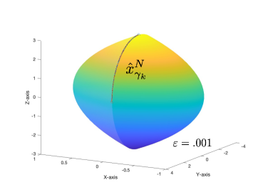
Figure 2: Exact optimal trajectory $\bar{x}$ vs Numerical optimal trajectory $\hat{x}_{\gamma_{k}}^{N}$

7 Conclusions

In this work, we successfully established a numerical method to solve optimal control problems involving sweeping processes, in which the sweeping set is not necessarily smooth, that is, it is defined as the intersection of a finite number of sublevel sets of smooth functions. It is worth mentioning that nonsmooth sweeping sets, including polyhedrals, are known to occur naturally in applications.

In addition to proving the convergence of our algorithm to an optimal trajectory for the problem, we further confirmed the high effectiveness and efficiency of our numerical method by providing an example, for which we calculated, on one hand, an exact optimal solution via the maximum principle of verachadijca , and, on the other hand, a numerical optimal trajectory via our algorithm. It is remarkable that the approximated trajectory and the exact one turned out to be almost identical, and the error in the objective functions is $.03$, after running the algorithm for only 183 seconds.

This numerical method is a generalization to the nonsmooth setting of the numerical algorithm in pinhonum ; verachadinum developed for smooth sweeping sets. As opposed to the latter, a number of serious challenges are encountered in this paper. The nonsmooth property of the maximum function defining our sweeping set posed a major obstacle that prohibited using the technique employed in the smooth setting. To overcome this significant obstacle, we used original and new techniques, including a well constructed smooth approximation of the maximum function defining the sweeping set, and two different, but equivalent, representations of the standard control system that approximates the controlled sweeping process of the original problem.

Extensions of our numerical method to cover more classes of optimal control problems over sweeping processes, such as time dependent nonsmooth sweeping sets, will be the subject of future research.

References

- (1) Adam, L., Outrata, J.: On optimal control of a sweeping process coupled with an ordinary differential equation. Discrete Contin. Dyn. Syst. B 19, 2709-2738 (2014)
- (2) Brokate, M., Krejčí, P.: Optimal control of ODE systems involving a rate independent variational inequality. Discrete and continuous dynamical systems series B 18, 331-348 (2013)
- (3) Brudnyi, A., Brudnyi, Y.: Methods of Geometric Analysis in Extension and Trace Problems, Volume 1, Monographs in Mathematics, 102. Birkhäuser/Springer Basel AG, Basel (2012)
- (4) Cao, T.H., Colombo, G., Mordukhovich, B., Nguyen, D.: Optimization of Fully Controlled Sweeping Processes. J. Differ. Equ. 295, 138-186 (2021)
- (5) Cao, T.H., Colombo, G., Mordukhovich, B., Nguyen, D.: Optimization and discrete approximation of sweeping processes with controlled moving sets and perturbations, J. Differ. Equ. 274, 461-509 (2021)
- (6) Cao, T.H., Mordukhovich, B.: Optimal control of a perturbed sweeping process via discrete approximations. Discrete Contin. Dyn. Syst. Ser. B 21, 3331-3358 (2016)
- (7) Cao, T.H., Mordukhovich, B.: Optimality conditions for a controlled sweeping process with applications to the crowd motion model. Disc. Cont. Dyn. Syst. Ser. B 22, 267-306 (2017)
- (8) Cao, T.H., Mordukhovich, B.: Optimal control of a nonconvex perturbed sweeping process. J. Differ. Equ. 266. 1003-1050 (2019)
- (9) Clarke, F.H.: Optimization and Nonsmooth Analysis, John Wiley, New York (1983)
- (10) Clarke, F.H., Stern, R.J., Wolenski, P.R.: Proximal smoothness and the lower- property. J. Convex Anal. 2, 117-144 (1995)
- (11) Clarke, F.H., Ledyaev, Yu., Stern, R.J., Wolenski, P.R: Nonsmooth Analysis and Control Theory. Graduate Texts in Mathematics, 178, Springer-Verlag, New York (1998)
- (12) Colombo, G., Henrion, R., Hoang, N.D., Mordukhovich, B.S.: Optimal control of the sweeping process, Dyn. Contin. Discrete Impuls. Syst. Ser. B 19, 117-159 (2012)
- (13) Colombo, G., Henrion, R., Hoang, N.D., Mordukhovich, B.S.: Optimal control of the sweeping process over polyhedral controlled sets, J. Differ. Equ. 260(4), 3397-3447 (2016)
- (14) Colombo, G., Mordukhovich, B., Nguyen, D.: Optimization of a perturbed sweeping process by constrained discontinuous controls, SIAM Journal on Control and Optimization, 58 no. 4, 2678-2709 (2020)
- (15) Delfour, M.C., Zolésio, J.-P.: Shapes and Geometries, Metrics, Analysis, Differential Calculus, and Optimization. Second edition, Advances in Design and Control, vol. 22, Society for Industrial and Applied Mathematics (SIAM), Philadelphia PA (2011)
- (16) de Pinho, M.d.R., Ferreira, M.M.A., Smirnov, G.V.: Optimal Control Involving Sweeping Processes, Set-Valued Var. Anal. 27, no. 2, 523–548 (2019)
- (17) de Pinho, M.d.R., Ferreira, M.M.A., Smirnov, G.V.: Correction to: Optimal Control Involving Sweeping Processes. Set-Valued Var. Anal. 27, 1025-1027 (2019)
- (18) de Pinho, M.d.R., Ferreira, M.M.A., Smirnov, G.V.: Optimal Control with Sweeping Processes: Numerical Method. J Optim Theory Appl. 185, 845-858 (2020)
- (19) de Pinho, M.d.R., Ferreira, M.M.A., Smirnov, G.V.: Necessary conditions for optimal control problems with sweeping systems and end point constraints. Optimization, 71:11, 3363-3381 (2021)
- (20) de Pinho, M.d.R., Ferreira, M.M.A., Smirnov, G. A: Maximum Principle for Optimal Control Problems Involving Sweeping Processes with a Nonsmooth Set. J Optim Theory Appl. 199, 273-297 (2023)
- (21) Henrion, R., Jourani, A., Mordukhovich, B.S: Controlled polyhedral sweeping processes: Existence, stability, and optimality conditions, J. Differ. Equ. 366, 408-443 (2023)
- (22) Hermosilla, C., Palladino, M.: Optimal Control of the Sweeping Process with a Nonsmooth Moving Set, SIAM Journal on Control and Optimization. 60:5, 2811-2834 (2022)
- (23) Hiriart-Urruty, J.-B., Strodiot, J.-J., Nguyen, V. H.: Generalized Hessian matrix and second-order optimality conditions for problems with data. Appl. Math. Optim. 11 no. 1, pp. 43-56 (1984)
- (24) Li, X.-S., Fang, S.-C.: On the entropic regularization method for solving min-max problems with applications, Math. Methods Oper. Res. 46, 119-130 (1997)
- (25) Mordukhovich, B.S.: Variational Analysis and Generalized Differentiation, I: Basic Theory, Springer, Berlin (2006)
- (26) Moreau, J.J.: Rafle par un convexe variable, I, Trav. Semin. d’Anal. Convexe, Montpellier 1, Exposé 15, 36 pp. (1971)
- (27) Moreau, J.J.: Rafle par un convexe variable, II, Trav. Semin. d’Anal. Convexe, Montpellier 2, Exposé 3, 43 pp. (1972)
- (28) Moreau, J.J.: Evolution problem associated with a moving convex set in a Hilbert space, J. Differ. Equ. 26, 347-374 (1977)
- (29) Nour, C., Zeidan, V.: Optimal control of nonconvex sweeping processes with separable endpoints: Nonsmooth maximum principle for local minimizers. J. Differ. Equ. 318, 113-168 (2022)
- (30) Nour, C., Zeidan, V.: Numerical solution for a controlled nonconvex sweeping process. IEEE Control Syst. Lett. 6, 1190-1195 (2022)
- (31) Nour, C., Zeidan, V.: A Control Space Ensuring the Strong Convergence of Continuous Approximation for a Controlled Sweeping Process. Set-Valued Var. Anal. 31, 23 (2023)
- (32) Nour, C., Zeidan, V.: Nonsmooth optimality criterion for a W1,2-controlled sweeping process: Nonautonomous perturbation. Applied Set-Valued Analysis and Optimization 5(2), 193-212 (2023)
- (33) Nour, C., Zeidan, V.: Pontryagin-Type Maximum Principle for a Controlled Sweeping Process with Nonsmooth and Unbounded Sweeping Set. J. Convex Anal. 31, (2024), to appear.
- (34) Rockafellar, R.T., Wets, R.J.-B.: Variational analysis. Grundlehren der Mathematischen Wissenschaften, 317, Springer-Verlag, Berlin (1998)
- (35) Thibault, L.: Unilateral Variational Analysis in Banach Spaces. World Scientific (2023)
- (36) Zeidan, V., Nour, C., Saoud, H.: A nonsmooth maximum principle for a controlled nonconvex sweeping process. J. Differ. Equ. 269(11), 9531-9582 (2021)